Image Summarisation:

Human Action Description from Static Images

Eleni Tsironi

Dissertação

Mestrado Internacional em Processamento de Linguagem Natural

e Indústrias da Língua

International Masters in Natural Language Processing

and Human Language Technology

Trabalho efetuado sob a orientação de:Prof. Doutor Jorge Manuel Evangelista Baptista (Universidade do Algarve)

Prof. Henri Madec (Université de Franche-Comté)Dr. Constantin Orăsan, University of Wolverhampton (University of Wolverhampton)

Faro - 2014

Image Summarisation: Human Action Description from Static Images

Declaração de autoria do trabalho

Declaro ser o(a) autor(a) deste trabalho, que é original e inédito. Autores e trabalhos consultados estão devidamente citados no texto e constam da listagem de referências incluída.

© 2014, Eleni Tsironi / Universidade do Algarve

A Universidade do Algarve tem o direito, perpétuo e sem limites geográficos, de arquivar e publi-citar este trabalho através de exemplares impressos reproduzidos em papel ou de forma digital, ou por qualquer outro meio conhecido ou que venha a ser inventado, de o divulgar através de reposi-tórios científicos e de admitir a sua cópia e distribuição com objetivos educacionais ou de investi-gação, não comerciais, desde que seja dado crédito ao autor e editor.

ii

To my beloved parents, Antonia and Fotis,for their support in every step of my life

and Robby, my little xaxaki.

iii

iv

Acknowledgements

First of all, I would like to express my sincere gratitude to the Erasmus Mundus Program and European Commission for the scholarship they awarded me, giving me the opportunity to study this interesting masters program.

Secondly, I would like to thank the University of Wolverhampton, Université de Franche-Comté, Toyohashi University of Technology, Universidade do Algarve, and all the professors and lecturers, for their knowledge and guidance during those two year. I would especially like to thank the coordinator Sylviane Cardey Greenfield and Gabriel Secondat for making sure that everything during the two years of our studies worked properly.

Consequently, I would like to express my deepest thanks to my three supervisors Prof. Jorge Baptista, Prof. Henri Madec and Dr. Constantin Oraŝan for their useful guidance and their advices.

I would like to specially thank my friends Robertus Paulus Hegge and José Luis Vieyra Sagaón, who first of all supported me psychologically during my work, but also with their technical help and knowledge during the development of the annotation platform. I should also thank Robertus Paulus Hegge for his participation as an assessor during the manual evaluation of my system and my friend Vlad Niculae for the interesting discussions with him, his bright ideas and his inspiration, that influenced the way to develop my methodology.

I would like to thank all the friends and people that volunteered to participate in the annotation project, without the contribution of whom it would have been impossible to complete this project.

Finally, I thank my parents for their support during every step in my life and their trust in my capabilities and especially thanks to my mother for her contribution during the manual evaluation of the system.

v

Abstract

The object of this master thesis is Image Summarisation and more specifically the automatic human action description from static images. The work has been organised into three main phases, with first one being the data collection, second the actual system implementation and third the system evaluation. The dataset consists of 1287 images depicting human activities belonging in fours semantic categories; "walking a dog", "riding a bike", "riding a horse" and "playing the guitar". The images were manually annotated with an approach based in the idea of crowd sourcing, and the annotation of each sentence is in the form of one or two simple sentences.

The system is composed by two parts, a Content-based Image Retrieval part and a Natural Language Processing part. Given a query image the first part retrieves a set of images perceived as visually similar and the second part processes the annotations following each of the images in order to extract common information by using a graph merging technique of the dependency graphs of the annotated sentences. An optimal path consisting of a subject-verb-complement relation is extracted and transformed into a proper sentence by applying a set of surface processing rules.

The evaluation of the system was carried out in three different ways. Firstly, the Content-based Image Retrieval sub-system was evaluated in terms of precision and recall and compared to a baseline classification system based on randomness. In order to evaluate the Natural Language Processing sub-system, the Image Summarisation task was considered as a machine translation task, and therefore it was evaluated in terms of BLEU score. Given images that correspond to the same semantic as a query image the system output was compared to the corresponding reference summary as provided during the annotation phase, in terms of BLEU score. Finally, the whole system has been qualitatively evaluated by means of a questionnaire.

The conclusions reached by the evaluation is that even if the system does not always capture the right human action and subjects and objects involved in it, it produces understandable and efficient in terms of language summaries.

Keywords

image summarisation, image description, content-based image retrieval, information extraction, sentence generation

vi

Resumo

O objetivo desta dissertação é sumarização imagem e, mais especificamente, a geração automática de descrições de ações humanas a partir de imagens estáticas. O trabalho foi organizado em três fases principais: a coleta de dados, a implementação do sistema e, finalmente, a sua avaliação. O conjunto de dados é composto por 1.287 imagens que descrevem atividades humanas pertencentes a quatro categorias semânticas: "passear o cão", "andar de bicicleta", "andar a cavalo" e "tocar guitarra". As imagens foram anotadas manualmente com uma abordagem baseada na ideia de 'crowd-sourcing' e a anotação de cada frase foi feita sob a forma de uma ou duas frases simples.

O sistema é composto por duas partes: uma parte consiste na recuperação de imagens baseada em conteúdo e a outra parte, que envolve Processamento de Língua Natural. Dada uma imagem para procura, a primeira parte recupera um conjunto de imagens percebidas como visualmente semelhantes e a segunda parte processa as anotações associadas a cada uma dessas imagens, a fim de extrair informações comuns, usando uma técnica de fusão de grafos a partir dos grafos de dependência das frases anotadas. Um caminho ideal consistindo numa relação sujeito-verbo-complemento é então extraído desses grafos e transformado numa frase apropriada, pela aplicação de um conjunto de regras de processamento de superfície.

A avaliação do sistema foi realizado de três maneiras diferentes. Em primeiro lugar, o subsistema de recuperação de imagens baseado em conteúdo foi avaliado em termos de precisão e abrangência (recall) e comparado com um limiar de referência (baseline) definido com base num resultado aleatório. A fim de avaliar o subsistema de Processamento de Linguagem Natural, a tarefa de sumarização imagem foi considerada como uma tarefa de tradução automática e foi, portanto, avaliada com base na medida BLEU. Dadas as imagens que correspondem ao mesmo significado da imagem de consulta, a saída do sistema foi comparada com o resumo de referência correspondente, fornecido durante a fase de anotação, utilizando a medida BLEU. Por fim, todo o sistema foi avaliado qualitativamente por meio de um questionário.

Em conclusão, verificou-se que o sistema, apesar de nem sempre capturar corretamente a ação humana e os sujeitos ou objetos envolvidos, produz, no entanto, descrições compreensíveis e e linguisticamente adequadas.

Palavras-chavesumarização automática de imagem, descrição automática de imagem, recuperação de imagens baseada em conteúdo, extração de informação, geração de frases

vii

Resumo Alargado

O objetivo desta dissertação é sumarização imagem e, mais especificamente, a geração automática de descrições de ações humanas a partir de imagens estáticas. O trabalho foi organizado em três fases principais: a coleta de dados, a implementação do sistema e, finalmente, a sua avaliação. O conjunto de dados é composto por 1.287 imagens que descrevem atividades humanas pertencentes a quatro categorias semânticas: "passear o cão", "andar de bicicleta", "andar a cavalo" e "tocar guitarra". As imagens foram anotadas manualmente com uma abordagem baseada na ideia de 'crowd-sourcing' e a anotação de cada frase foi feita sob a forma de uma ou duas frases simples.

O sistema é composto por duas partes: A primeira parte do sistema é um sistema de recuperação de imagem baseada em conteúdo que procura imagens com conteúdo visual similar. Durante a fase de treino, as imagens utilizadas como conjunto de treino são segmentadas pelo algoritmo de segmentação baseada em grafos de Felzenszwalb e Huttenlocher. Antes de o processo de segmentação, todas as imagens são convertidas para miniaturas (thumbnails), a fim de reduzir o conteúdo de informação e, por conseguinte, o ruído na imagem, tentando, no entanto, captar as estruturas/formas mais importantes na mesma. Cada região segmentada é representada por um vector de traços de momentos Hu, que são invariantes relativamente à tradução, rotação e escala. Finalmente, todos os vetores de traços que correspondem aos segmentos da imagem são utilizados para treinar um classificador utilizando o algoritmo do vizinho K mais próximo.

Quando uma imagem desconhecida ou para procura é dada ao sistema a fim de ser automaticamente resumida (ou, por outras palavras, para receber uma descrição), ela é submetida ao mesmo procedimento utilizado para as imagens de treino. Por outras palavras, a imagem é convertida numa miniatura e é segmentado pelo algoritmo de Felzenszwalb e Huttenlocher; em seguida, são calculados os momentos Hu para cada uma das suas regiões segmentadas. Os vectores de traços, que correspondem a cada imagem são mapeados para o classificador previamente treinado e para cada vector de traços recupera-se o nome da imagem correspondente ao segmento de imagem mais semelhante. Uma vez que o número de imagens recuperadas é relevante para o número de segmentos de uma imagem, este último pode tornar-se muito elevado. É óbvio, também, que, se uma imagem é segmentada em muitas regiões, nem todos elas estão relacionadas com os objetos ou segmentos que capturam na imagem a ação humana a descrever e, portanto, aplica-se um processo de seleção.

As imagens obtidas são classificadas de acordo com sua pontuação de similaridade em ordem crescente e as primeiras 26 imagens são escolhidas para a próxima etapa de seleção. O número de imagens foi empiricamente ajustado, após várias experiências. As imagens recuperadas têm um nome que as classifica em cada uma das quatro categorias em que consiste o conjunto de treino. As imagens são, então, agrupadas de acordo com a ação em que foram classificadas, denotada a partir do seu nome, e o conjunto de imagens correspondentes à classe com a frequência mais baixa é recuperada como similar.

Durante a fase seguinte, o conjunto de imagens semelhantes recuperados é fornecido ao subsistema de processamento de linguagem natural. As imagens já não são mais processadas, mas seus resumos, recolhidos durante a fase de anotação, são nesta altura processados a fim de deles

viii

se extrair a informação comum, que será utilizado para produzir o resumo (ou descrição) para a imagem de consulta. Cada uma das frases que correspondem às imagens recuperadas é analisada pelo analisador sintático de Stanford e representada em forma de gráfico de dependências, onde os nós são as palavras com sua categoria morfossintática (part-of-speech) e as transições são nomeadas com dependências de Stanford abreviadas.

O passo seguinte é a fase de fusão dos grafos, durante o qual os grafos de dependência dos passos anteriores são unidos de acordo com os seus nós e transições comuns para formar um grafo ou grafos maiores. A fim de fundir um nó com outro nó, estes são comparados uns com os outros. Os nós estão marcados com o nome da palavra, bem como a respetiva categoria morfossintática. Se as etiquetas são as mesmas, então os nomes dos nós são comparados como simples cadeias de caracteres. Se forem idênticos, os nós são fundidos e um peso correspondente aos nós é atualizado para indicar a frequência da palavra.

O mesmo procedimento é seguido para as transições. As transições que compartilham a mesma etiqueta e conectam os mesmos nós também são fundidas e o seu peso é atualizado de acordo com suas frequências. Por causa da natureza do texto a ser processado para esta tarefa específica, adoptou-se como principal hipótese quanto à informação mais importante a noção de que é o verbo que captura a ação principal retratada na imagem e, portanto, a fim de fundir os gráficos, adota-se além disso uma outra estratégia. Neste caso, os nós rotulados como substantivos que são o sujeito e o objecto do verbo são examinados quanto à sua similaridade semântica.

Por outras palavras, os nós que são extraídos pelo analisador como sujeitos de um dado verbo constituem um conjunto, e os seus membros são comparados uns com os outros com o recurso à WordNet, a fim de identificar se estão semanticamente relacionados. Essa relação semântica é aqui identificada quando os dois nós compartilham um hiperónimo comum. O mesmo processo é repetido para os objetos diretos, a fim de verificar se existem nós que podem ser fundidos através da sua hiperonímia comum. No caso de verbos, um processo lematização é utilizado, a fim de verificar se há lemas comuns entre as duas palavras. Se os nós compartilham o mesmo lema, são então fundidos e suas dependências para outros nós também são atualizadas, bem como seus respetivos pesos.

Assim que todos os gráficos se encontram fundidos, é extraído um caminho ideal sujeito-verbo-complemento. Como se disse atrás, assume-se que os verbos são os elementos responsáveis por transmitir a ação principal retratada numa imagem. Outra suposição é a de que, para que a ação esteja completa, deve haver um complemento do verbo. O complemento do verbo é definido como quer o complemento direto ou indireto (preposicional) do verbo.

A partir da anterior fusão dos grafos, temos agora um ou mais grafos, os nós e as transições, ponderados em função da soma de suas frequências nos seus respectivos subgrafos. Para extrair o verbo que descreve a ação principal na imagem de consulta, as transições com as relações verbo-objeto direto são ordenadas de acordo com suas frequências. Posteriormente, a transição com a maior frequência é extraída. Em caso de falta de uma relação verbo-objeto direto nos grafos, o que significa que não há objetos diretos como complementos do verbo, os objetos indiretos dos verbos são de seguida ordenados de acordo com os respetivos pesos. Também neste caso é extraída a relação ponderada com a maior frequência.

ix

A extração de uma relação verbo-objeto direto ou verbo-objeto indireto visa garantir a extração de um verbo e do seu complemento. As relações verbo-sujeito correspondente ao verbo extraídos são ordenadas de acordo com seus pesos e o sujeito com a maior pontuação é extraído como o sujeito da nova imagem. Considera-se, então, que o caminho ideal sujeito-verbo-complemento foi extraído com sucesso. Uma vez que a saída desejável do sistema é de uma forma de frase, o caminho extraído passa então por uma fase de tratamento de superfície. Em primeiro lugar, o sistema verifica o número do sujeito extraído e, de acordo com este, atribui-lhe um determinante e flexiona o verbo. O pressuposto é o de que, se o substantivo se encontra no singular, atribui-se-lhe o artigo indefinido "a" ou "an" (um/uma/uns/umas) de acordo com a forma do nome, ao passo que, no plural, se emprega a pronome indefinido "some" (alguns/etc.). Finalmente, o artigo definido "the" (o/a/os/as) é atribuído diante do complemento do verbo.

Todos os elementos básicos que são necessários para formar a frase são selecionados e são colocados na ordem certa. Esta ordem é, em primeiro lugar, o determinante do sujeito, o sujeito e o verbo; finalmente, se o objeto extraído for um complemento direto, então, coloca-se o seu determinante e o objeto; caso contrário, se se trata de uma relação indireta, a preposição, o determinante e objeto são colocados no final da frase.

A avaliação do sistema foi realizado de três maneiras diferentes. Em primeiro lugar, o subsistema de recuperação de imagens baseado em conteúdo foi avaliado em termos de precisão e abrangência (recall) e comparado com um limiar de referência (baseline) definido com base num resultado aleatório. A fim de avaliar o subsistema de Processamento de Linguagem Natural, a tarefa de sumarização imagem foi considerada como uma tarefa de tradução automática e foi, portanto, avaliada com base na medida BLEU. Dadas as imagens que correspondem ao mesmo significado da imagem de consulta, a saída do sistema foi comparada com o resumo de referência correspondente, fornecido durante a fase de anotação, utilizando a medida BLEU. Por fim, todo o sistema foi avaliado qualitativamente por meio de um questionário.

Em conclusão, verificou-se que o sistema, apesar de nem sempre capturar corretamente a ação humana e os sujeitos ou objetos envolvidos, produz, no entanto, descrições compreensíveis e e linguisticamente adequadas.

x

Table of Contents1 Introduction...................................................................................................................................1

1.1 Topic.......................................................................................................................................11.2 Aims ......................................................................................................................................11.3 Research questions ................................................................................................................21.4 Rationale ...............................................................................................................................21.5 Thesis Outline........................................................................................................................3

2 Related work..................................................................................................................................52.1 Image Annotation - From Image to Words ...........................................................................52.2 Image Descriptions - From Image to Text ............................................................................82.3 Other Description Systems .................................................................................................12

2.3.1 Systems Incrementally Describing Image Sequences .................................................122.3.2 Video Descriptions ......................................................................................................13

2.4 Discussion & Conclusions ..................................................................................................143 Methodology................................................................................................................................15

3.1 Overview..............................................................................................................................153.2 Dataset..................................................................................................................................17

3.2.1 Image Collection..........................................................................................................173.2.2. Annotation Guidelines.................................................................................................183.2.3. Demographic Analysis................................................................................................193.2.4. Annotation Evaluation - Error Correction and Error Analysis ...................................20

3.2.4.2.1 Causes of Errors................................................................................................223.2.4.2.2. Error handling ..................................................................................................23

3.3 Image Retrieval....................................................................................................................253.3.1 Text-based Image Retrieval versus Content-based Image Retrieval............................253.3.2 Computer Vision - Image Processing...........................................................................25

3.3.2.1 Image Segmentation.............................................................................................263.3.2.2 Image Descriptors ................................................................................................333.3.2.3 Similarity Measures..............................................................................................40

3.3.3 Content-based Image Retrieval System - Proposed method........................................443.4 Natural Language Processing .............................................................................................46

3.4.1 Overview of Computational Linguistics & Natural Language Processing..................463.4.2 Syntax in Language......................................................................................................49

3.4.2.1 Constituency Theory ............................................................................................493.4.2.2 Dependency Theory..............................................................................................493.4.2.3 Syntactic Parsing..................................................................................................50

3.4.3 Lexical Semantics and Word Sense Disambiguation...................................................593.4.3.1 Knowledge Organisation Systems........................................................................59

3.4.4 Information Extraction.................................................................................................633.4.5 Natural Language Processing System - Proposed method...........................................64

3.4.5.1 Dependency parsing.............................................................................................643.4.5.2 Graph merging......................................................................................................643.4.5.3 Optimal path extraction........................................................................................663.4.5.3 Surface processing................................................................................................67

xi

4 Evaluation....................................................................................................................................694.1 Evaluation Overview...........................................................................................................69

4.1.2 Evaluation versus Verification.....................................................................................694.1.2.1 Black box, Glass box, Modular Evaluation..........................................................69

4.1.3 Kinds of Evaluation in Natural Language Processing.................................................704.1.3.1 Automatic versus Manual.....................................................................................704.1.3.2 Intrinsic versus Extrinsic......................................................................................704.1.3.3 Qualitative versus Quantitative Evaluation..........................................................704.1.3.4 Kinds of Evaluation according to EAGLES.........................................................704.1.3.5 Lower Bound versus Upper Bound......................................................................70

4.1.4 Eye-tracking in Natural Language Processing Evaluation...........................................714.1.5 Evaluation in Natural Language Generation................................................................71

4.1.5.1 GLEU...................................................................................................................714.1.6 Machine Translation Evaluation...................................................................................71

4.1.6.1 BLEU - Automatic Machine Translation Evaluation...........................................724.1.6.2 Manual Qualitative Evaluation in Machine Translation - EuroMatrix.................724.1.6.2.1 Fluency and adequacy ......................................................................................72

4.2 Evaluation of the proposed System .....................................................................................734.2.1 Evaluation of Content-based Image Retrieval System.................................................73

4.2.1.1 CBIR Evaluation Metrics.....................................................................................744.2.1.2 Confusion Matrix..................................................................................................744.2.1.2 CBIR System Evaluation......................................................................................75

4.2.2 Evaluation of Natural Language Processing System...................................................804.2.2.1 Error Analysis.......................................................................................................82

4.2.3 Overall System Qualitative Evaluation........................................................................834.2.3.1 Inter-annotator agreement.....................................................................................834.2.3.2 Questionnaire Objectives......................................................................................844.2.3.3 Cognitive metric scales.........................................................................................854.2.3.4 Questionnaire Results - Analysis..........................................................................85

4.3 Discussion on the Results....................................................................................................945 Summary & Conclusions.............................................................................................................97References ......................................................................................................................................99APPENDIX I................................................................................................................................113APPENDIX II ..............................................................................................................................117APPENDIX III.............................................................................................................................121APPENDIX IV.............................................................................................................................123

xii

Index & Referencing of Tables

Table 1: Errors per category in absolute numbers and in percentages. Table 2: Errors in respect to age bins. Table 3: Semantic Relations in WordNet. Retrieved from: [147]Table 4: Classification Accuracy for different numbers of retrieved images. Table 5: Confusion matrix & measures for the class "playing the guitar". Table 6: Confusion matrix & measures for the class "riding a bike". Table 7: Confusion matrix & measures for the class "walking the dog". Table 8: Confusion matrix & measures for the class "riding a horse". Table 9: BLEU score Distribution for the modified descriptions as training and testing set. Table 10: BLEU score Distribution for the original descriptions as training and testing set. Table 11: Intra-annotator Agreement.Table 12: Kappa Q3, Q4, Q6.Table 13: The distribution of the overall system evaluation per assessor. Table 14: The distribution of the human activity recognition per assessor.Table 15: The distribution of subject and object recognition per assessor.Table 16: The distribution of the language fluency per assessor.Table 17: The distribution of grammatical error evaluation per assessor.Table 18: The distribution of lexical error evaluation per assessor.Table 19: The distribution of sentence completeness per assessor.Table 20: The distribution of sentence clarity per assessor.

xiii

Index & Referencing of Figures

Figure 1: System Overview. Figure 2: Stanford dataset. Retrieved from: http://vision.stanford.edu/Datasets/40actions.html Figure 3: Willow Actions. Retrieved from: http://www.di.ens.fr/willow/research/stillactions/Figure 4: Number of images annotated per annotator. Figure 5: Distribution of annotators in respect to their age. Figure 6: Distribution of each error category in relation to the total amount of errors. Figure 7: Thresholding segmentation. Retrieved from: http://docs.opencv.org/doc/tutorials/imgproc/threshold/threshold.html Figure 8: Segementation with k-means. Retrieved from: http://ij-plugins.sourceforge.net/plugins/segmentation/k-means.html Figure 9: Compression-based methods. Retrieved from: [34] Figure 10: Watershed Transformation. 10(a): Retrieved from: http://www.mathworks.com/help/images/examples/marker-controlled-watershed-segmentation.html 10(b): Retrieved from: [194] 10(c): Retrieved from: [59] Figure 11: Watershed segmentation with markers. Retrieved from: http://www.mathworks.com/help/images/examples/marker-controlled-watershed-segmentation.html Figure 12: Canny Edge Detector. Retrieved from: http://www-scf.usc.edu/~boqinggo/Canny.htm Figure 13: Region Growing Segmentation. Retrieved from: http://en.wikipedia.org/wiki/Region_growing Figure 14: Splitting and merging. Retrieved from: http://homepages.inf.ed.ac.uk/rbf/CVonline/LOCAL_COPIES/MARBLE/medium/segment/split.htm Figure 15: Segmentation using snakes. Retrieved from: http://en.wikipedia.org/wiki/Active_contour_model Figure 16: Level Set Segmentation. Retrieved from: [195] Figure 17: left IKONOS imagery, right SOM segmentation. Retrieved from: [196]Figure 18: Segmentation with Felzenszwalb and Huttenlocher approach. Retrieved from: [49] Figure 19: Colour Layout Descriptors. Retrieved from: http://en.wikipedia.org/wiki/Colour_layout_descriptor Figure 20: An overview of shape description techniques Retrieved from:[46 p.258] Figure 21: left: Manhattan, right: distance Euclidean distance. Figure 22: Cosine similarity:(a) Similar scores, (b) Unrelated scores, (c) Opposite scores. Figure 23: Example of k-neighbours classification; 3 training instances vote for a query instance. Retrieved from: http://horicky.blogspot.pt/2012/06/predictive-analytics-neuralnet-bayesian.html Figure 24: Overview of the Content-based Image Retrieval system. Figure 25: Language Production versus Language Comprehension. Figure 26: The stages of processing in analysis in Natural Language Processing.[87] Figure 27: Representation corresponding to constituency grammar. Retrieved from: [93] Figure 28: Representation corresponding to Dependency Analysis. Retrieved from [93]

xiv

Figure 29: Stanford collapsed dependencies. Retrieved from: http://nlp.stanford.edu/software/stanford-dependencies.shtml Figure 30: Stanford dependencies. Retrieved from: http://nlp.stanford.edu/software/stanford-dependencies.shtml Figure 31: A taxonomy of animals. Retrieved from: http://www0.cs.ucl.ac.uk/staff/a.hunter/tradepress/tax.html Figure 32: Thesaurus representation; Relations between concepts. Retrieved from: https://grips.semantic-web.at/display/public/POOLDOKU/Thesaurus+Basics Figure 33: An excerpt of the WordNet semantic network. Retrieved from: [130],graph page 10:9 Figure 34: Dependency Representation of all the texts corresponding to the similar retrieved images to the query image on the left.Figure 35: Cut of the merged graph from which the optimal path is extracted. Figure 36: Confusion matrix. Retrieved from: http://uberpython.wordpress.com/2012/01/01/precision-recall-sensitivity-and-specificity/ Figure 37: Segmentation Results for the class "walking the dog".Figure 38: Segmentation Results for the class "riding a horse".Figure 39: Segmentation Results for the class "riding a bike".Figure 40: Segmentation Results for the class "playing the guitar".Figure 41: BLEU score Distribution for the original descriptions. Figure 42: BLEU score Distribution for the modified descriptions. Figure 43: The distribution of the overall system evaluation per assessor. Figure 44: The distribution of the human activity recognition per assessor.Figure 45: The distribution of subject and object recognition per assessor. Figure 46: The distribution of the language fluency per assessor. Figure 47: The distribution of grammatical error evaluation per assessor.Figure 48: The distribution of lexical error evaluation per assessor.Figure 49: The distribution of sentence completeness per assessor. Figure 50: The distribution of sentence clarity per assessor.

xv

1 Introduction

1 Introduction

1.1 Topic

The current dissertation deals with the topic of Image Summarisation and more specifically with the description of human actions depicted in an image in form of text. A concrete definition of the term Image Summarisation is necessary before we go into detail about the approaches and methods used for the implementation of this project.

In the literature, the Image Summarisation systems can be used for several purposes. Their main feature is the fact that they are meant to summarise visually an image or a video. In other words, such a system gets as input either an image or a set of images or even an image sequence and produces as output a visual summary, which means that the output is also in the form of an image or several images[1][2]. Moreover, the term can be also found in the context of image data compression[3]. However, in the current research project, the summarisation of the image is addressed as the problem of the semantic interpretation of the image content in the form of text. For this reason, in order to avoid any eventual confusion between those research areas, the terms Image Textual Summarisation, Image Summarisation and Image Description are interchangeable and they all imply given a previously unseen image to the system a short summary in form of text is produced, describing the semantic content of it.

In the narrow sense, the current project deals with the summarisation of images depicting human actions. Therefore, the term of human action has to be clarified. According to some famous dictionaries and among the definitions of the word action, is defined as a physical movement(Cambridge dictionaries[191]) or as a gesture or movement(Oxford dictionaries[50]). Therefore, we can conclude that an action is a physical movement or gesture. This implies a change in the posture of the human body evolving in the time. As a consequence if we want to identify a human action we need a sequence of images that capture those changes in the body posture. However, this project is motivated by the fact that humans tend to recognise human actions and activities from static images and attempts to simulate this human highly cognitive task.

1.2 Aims

The main aim of this thesis is to develop a system that produces image descriptions of higher semantics. More specifically, descriptions that capture the main actions between the prominent objects(with the term objects both animate and inanimate image contents are meant e.g. any object, as well as any animal or humans) in an image. Given a query image as input to the system, the output has to be a textual summarisation of this specific input image.

The current project aims to successfully combine the two research fields of Content-based Image Retrieval(CBIR) and a Natural Language Processing, in order to develop a system, that will first

1

1 Introduction

search for visually similar images in an existing database and based on some annotated text that each of this images is accompanied, produce a short human understandable description about the content of the query image.

Therefore, among the purposes of this dissertation is the creation of a manually annotated image dataset, with the form of annotation being short descriptions about the content of the image. Since the goal of this dissertation is to simulate a higher cognitive task, a training set on actual data on how humans perceive images has to be collected.

Finally, this work also aims on a proper evaluation of the system with automatic as well as manual means. During the evaluation process, humans should be given the opportunity to judge whether a system like that fulfils its goals, in order to find out its weaknesses and strengths.

1.3 Research questions

The main research question of this project is How do humans extract actions from static images and how can this highly cognitive task can be simulated by a machine?. Thereupon:

• How can an image be automatically described without the use of a visual object database, that represents human knowledge?

• When are two images similar and how can we automatically achieve this task?

• How can we automatically extract the main objects in an image?

• How can we extract from the descriptions of similar images the common knowledge?

• How can we form a proper text for the query image?

• How can we properly evaluate such a system?

1.4 Rationale

A successful implementation of the Image Summarisation system in the broad sense can be useful in several research fields and for the development of several commercial applications. An eventual and very promising application in bioinformatics field could be the Automatic Description of Medical Images. In this case, of course, the system should be trained with the respective image data set. Automatic Diagnosis from MRI (Magnetic Resonance Imaging) could be an interesting and very useful application. More specifically, the system would retrieve MR images from similar cases and analyse the text diagnosis which follows each of them in order to produce a diagnosis of the query MR image. This could be a very powerful field of application since the text written by the doctors, describes those images without including any noisy information, in contrast to an application where the training picture dataset is described by higher semantic interpretations and personal experiences of the user, which may not correspond to the content of the picture. The system could be considered as a very helpful tool for doctors that saves them time during the diagnosis process.

2

1 Introduction

In addition, the system could be a great tool for blind people or people with other visual disabilities. While surfing the web, those users do still face difficulties in the interpretation of images, since not all of them are followed by meta-data or descriptions that can clearly convey the meaning of the picture to the user. What is more, the Image Summarisation system in combination with an Optical Character Recognition system and a Speech Synthesis System could be a very useful tool for the complete interpretation of scanned documents containing pictures.

Furthermore, nowadays, it is very easy and cheap to capture photographs. It is very common that people owe big disorganised collections of photographs in digital form. Images can be a great source of information. Consequently, such a system could be a tool for better organisation of the image set and therefore their retrieval based on text queries.

Last but not least, as an extension of the previous application, an Image Summarisation system could be used in image retrieval indexing by search engines in the World Wide Web for the better performance of the image retrieval with the use of text queries.

1.5 Thesis Outline

As already mentioned before, the task of this project is the automatic description of images depicting human actions. This task has some major limitations since the actions are to be identified from still images and not from image sequences. As a consequence the action must be inferred as a result of the objects involved in the image and the relations of their poses. The main idea to deal with this demanding task, is the use of captioned data, describing the main interpretation of the scene emphasising on the main action.

So that the system output is closer to that a human would produce while describing a picture the training dataset will be annotated by several humans. Moreover, the system has to be flexible, which means that no visual ontology or predefined categories will be used to name the detected objects and actions. The system has to to learn the visual content from the training images of the existing dataset.

This dissertation is organised in three big sections. In section 2, an overview of the related work is presenting, examining approached generating text output given an image, varying from simple words to proper descriptions. Section 3 presents the proposed method, while providing an overview of the state-of-the-art techniques out of which the selected ones where chosen for the completion of this project. The evaluation methods and the results of the system implementation are presented in Section 4.

3

1 Introduction

4

2 Related work

2 Related work

The purpose of this section is to present the related work to the broad sense of Image Description and Image Summarisation in the sense those terms were defined in the previous section. Since these tasks are very complicated and difficult, requiring a combination of two different research fields those of Image Processing and Natural Language Processing, not so much attention has been paid by the research community, in terms of treating the topic as an integration of those both research areas equally until the recent years. In the following sections the existing literature will be presented, the work done in the fields of Image Annotation and Image Description. Both notions of Image Annotation and Description have the same goal; given a digital picture as an input to the system, the output is a set of words. Of course, the descriptions differ in terms of more precise expression of the image content.

The first approaches gathering a lot of interest in the past is the group of methods that aim to convert an image to a set of unrelated words. As will be demonstrated in the next sections the output of these systems are words which may describe the image content pretty well but do not capture the semantic or spatial relationships of the image content. For example, considering the image of "a black bag on the table ", such a system produces as output the set of words {bag, black, table}. The words are isolated without expressing the semantic relationships between them. In this specific example, we can suppose from the output that there is a black bag on or under the table or a bag is under or next to or on a black table.

The problem of ambiguity in the interpretation of the output of such systems has been tried to solved in the more recent literature by enhancing the output so that it reveals those kind of spatial and semantic relationships. This approaches will be described in the section 2.2. Finally, in section 2.3 some other interesting approaches for Video Description systems will be briefly introduced. In the subsection 2.3.1 a category of methodologies for the description of image sequences, which depends on the concept of incrementally combining the image content and the language output. The proposed systems even if they are quite old, they deal with the simultaneous description of videos in a realistic time.

2.1 Image Annotation - From Image to Words

Plenty of work has been already done in Image Annotation and Image Captioning where specific regions of a given picture are associated to a specific word. Extensions to Image Annotation include Object Recognition in the picture and description of the spatial relationships between the recognised objects. Other approaches attempt not only to extract the objects but also their modifiers such as colour. Firstly, some of the approaches are presented in chronological order and then a sort discussion on them follows.

Y. Mori et al.[19] proposed in 1999 a method to identify a relationship between images and words. More specifically, each image is tagged with some words which are not necessarily restricted only to the objects depicted in the image. The method assumes that all the words

5

2 Related work

corresponding to the whole image can be inherited to sub-parts of it. In other words, the image is divided into equally rectangular parts, while each part is followed by all words tagged to the original image. From each of the sub-images a feature vector describing each specific segment is extracted carrying RGB colour histograms and histograms of intensity extracted after Sobel filtering. The extracted feature vectors are clustered by incremental vector quantisation. Thereafter, likelihoods for each word and each cluster centroid are estimated by accumulating their frequency. The system output for an unknown query image follows the previously described steps up to the mapping of each feature vector related to a specific sub-image to the closest centroid in the before-mentioned feature space. Thereafter, the average of the likelihoods of the nearest centroids are calculated and those words that have the highest likelihood values are combined to output the most plausible image caption.

Lavrenko et al.[24] in 2003, proposed a probabilistic model of learning the semantics of images that influenced many models proposed later on by the research community. This approach is based on the assumptions that the surrounding context often simplifies the interpretation of regions as a specific object and the association of different regions provides context while the association of words with image regions provides meaning. The formalism that models the generation of annotated images is a statistical generative model called Continuous-space Relevance Model. The proposed model computes a joint probability over different regions of some and the words in its annotation. Every image is divided into regions, each described by a continuous-valued feature vector reflecting the position of an object region, its relative size, a crude reflection of its shape, as well as predominant colours and textures. Given a training set of images with annotations, a joint probabilistic model of image features and words for the prediction of the probability of generating a word given the image regions is computed. The model proposed here directly associates continuous features with words.

P. Duygulu et al.[18] in 2004 proposed another clustering approach for image annotation. Given a training set of captioned images, the correlations between image features and keywords are trying to be discovered. The association between image regions and words is learnt from manually annotated images. An image region is represented by a vector of features regarding its colour, texture, shape, size and position. These feature vectors are clustered into clusters using the k-means algorithm while the number of clusters is adaptively defined using the G-means algorithm and each region is assigned the label of the closest cluster centre. These labels are called blob-tokens. The main idea is to give higher weight to terms/blob-tokens which are more "unique" in the training set, and low weights to noisy, common terms/blob-tokens. For the image captioning, several methods can be applied on a weighted translation table(to translate from the set of keywords of an image to the set of blobs forming the image), whose elements express the probability a term is captioned given a blob-token. The first proposed method is Corr, a correlation based method that measures the association between a term and a blob-token by the co-occurrence counts. The second method is called Cos and calculates instead a cosine-similarity translation table. Two last methods are also proposed the SvdCorr and SvdCos that generate the correlation translation table following the Singular Value Decomposition procedure instead of starting with the weighted data matrix.

6

2 Related work

Jiwoon Jeon and R. Manmatha[26] proposed in 2004 the use of the Maximum Entropy approach for the task of automatic image annotation. Given a set of labelled training data, Maximum Entropy is a statistical technique which allows to predict the probability of a label for a query. The query image is represented using a language of visual terms and then predict the probability of seeing an English word given the set of visual terms forming the image. Maximum Entropy computes the probability and in addition allows for the relationships between visual terms to be incorporated.

In 2006, Youakim Badr and Richard Chbeir[22] approached the image captioning problem, in other words the problem going from image to text but from another perspective, this of an image already surrounded by text, during the annotation process of which, the relevant information is extracted from the text in order to label the image. They introduced an expressiveness and extendible XML-based meta-model for Image Management, which is able to capture the meta-data and content-based features of images followed by text. The images in this case as already said, are surrounded by text and the goal is to create the appropriate meta-data to tag them from the text and from low-level visual features. The authors proposed an information extraction approach to provide automatic description of image content using the related meta-data. Their approach automatically generates XML instances, which mark up meta-data and salient objects matched by extraction patterns. For the specific example of image diagnosis meaningful data can be processed efficiently by regular expressions. The notation of regular expressions is extended by providing meta-words and a multilayer approach to define a high specification language for extraction patterns. The extraction patterns are mainly based on different meta-data permutations, expression disjunction and on the context to identify salient objects.

Sean Moran in 2009, in his dissertation[20] with the aim of developing more precise annotations, reimplemented the before-mentioned probabilistic model, the Continuous Relevance Model[24] proposed by Lavrenko, by extra considering the dependencies between keywords in order to eliminate the noisy ones. His main findings reveal that under certain conditions an effective method to increase annotation accuracy is obtained by enhancing the original Continuous Relevance Model the combination of keyword correlation with an beam search to examine over sets of tags. Moran’s proposed system starts with a pre-processing stage by forming a visual feature vector extracting colour, texture, shape and position information for every Normalised Cut segmented image region for every image in the training and test data sets. After the visual features have been extracted they are further processed to extract word frequency counts, standardise image features, compute all combinations of 2, 3 and 4 word queries and re-arrange the image features into data structures that allow fast processing within the model. The output of the feature pre-processing module is then fed into the Continuous Relevance Model which constructs a probability distribution to link the provided words and features and allow the actual automated image tagging and ranked retrieval. The initial tags assigned to the images can then be further refined by an optional beam search tag refinement module that seeks to find a near to optimal set of tags with high mutual correlation. The output number of words for every picture is predefined(e.g. predefined to 5 words).

7

2 Related work

Finally, in 2009, Luo Jie et al.[16] present an approach for the joint modelling of faces and poses in images and their association to names and action verbs in accompanying text captions. Given a corpus of news items consisting of images accompanied by text captions, the aim is to find out "who is doing what", as the authors state. In other words, names and action verbs in the captions are associated to the face and body pose of the people in the images. This joint model for simultaneously solving the image-caption correspondences and learning visual appearance models for the face and pose classes occurring in the corpus provides models that can then be used to recognise people and actions in novel images without captions. The connections between the subject and verb in a caption are found by language analysis techniques. Considering the subject-verb language construct, the "who is in the picture" and "who is doing what". The observed variables of this introduced generative model are names and verbs in the caption as well as detected persons in the image. The image-caption correspondences are carried by latent variables, while the visual appearance of face and pose classes corresponding to different names and verbs are model parameters. During learning, simultaneously the correspondence is solved and the appearance models are learnt. In this joint model, the correspondence ambiguity is reduced because the face and pose information help each other.

To conclude, this paragraph has presented some approaches on Image Annotation and Image Captioning. According to the organisation of this chapter, they are both techniques falling into the category From Image to Words. Both techniques produce text given an unseen image, however, Image Captioning requires as an input an image plus its surrounding text[22][16]. The words produced as the output of the system come from the surrounding text. However, Image Annotation does not require any textual input to the system that follows the input image. According to a trained model, such those introduced above, clustering[19][18], maximum entropy[19] or joint probability[20][24] a previously unseen image is labelled with some words produced by the system. The approaches may differ not only in the training models but also in the way they treat the image representation, such as division in rectangles[19] or meaningful segmentation[24].

2.2 Image Descriptions - From Image to Text

In this section, the approaches of generating coherent text out of images is presented. As the reader may notice below, this field has started very recently attracting the interest of the researchers. This section is also organised in chronological order and short discussion follows after the methods are presented.

Patrick Hède et al.[8] in 2004, proposed an image description system, which detects and recognises objects from a dictionary of objects indexed according to their visual characteristics(texture and colour) creating an image signature of its visual characteristics. The relative and absolute positions between the objects are also defined. The signatures of the detected objects are used to retrieve the keywords of the existing indexed objects in the visual dictionary. The description consists of the objects in the image, their attributes like colour,

8

2 Related work

brightness and the spatial relationships between the detected objects. For the final natural language generation part they use Named Entity Recognition and deep syntactical parsers.

Ali Farhadi et al.[4] in 2010 introduced a system that can compute a score linking an image to a sentence. This score can be used to attach a descriptive sentence to a given image, or to obtain images that illustrate a given sentence. The score is obtained by comparing an estimate of meaning obtained from the image to one obtained from the sentence. Each estimate of meaning comes from a discriminative procedure that is learned using data. The model assumes that there is a space of "Meanings" that comes between the space of "Sentences" and the space of "Images". First the similarity between a sentence and an image is evaluated by mapping each to the meaning space and then comparing the results. The mapping is learned from images to meaning and respectively from sentences to meaning discriminatingly from pairs of images and assigned meaning representations and sentences respectively. The "Meaning" space consists of triplets - object, action scene - and as a consequence the sentences have to get linguistically parsed in this form so that their visual features correspond to this triplet. For a query image, a matching procedure of it to the semantic space begins. If an image and a sentence predict very similar triplets, they should be projections of nearby points in the meaning space, and so they should have a high matching score. A natural noise resistant score of the similarity of sentence triplets and image triples is the sum of ranks of sentence meaning and image meaning. The pair with the smallest value of this sum is both predicted by the image and predicted by the sentence.

Benjamin Z. Yao et al.[11] in 2010 propose the I2T framework which generates text descriptions of image and video content based on image understanding. This framework is implemented in three steps. First, input images or video frames are decomposed into their constituent visual patterns by an image parsing engine. Afterwards, the image parsing results are converted into a semantic representation in the form of Web Ontology Language(OWL). Finally, a text generation engine converts the results from previous steps into semantically meaningful, human readable and query-able text reports. The core piece of the I2T framework is an And-Or Graph visual knowledge representation, which provides a graphical representation serving as prior knowledge for representing diverse visual patterns and provides top-down hypotheses during the image parsing. The And-Or Graph embodies vocabularies of visual elements including primitives, parts, objects, scenes as well as a stochastic image grammar that specifies syntactic relations and semantic relations between these visual elements. Therefore, the And-Or Graph is a unified model of both categorical and symbolic representation of visual knowledge.

Yansong Feng in his PhD thesis submitted in 2011 [25][10] focuses on the task of automatically generating captions for news images in a learning-from-data fashion, as called by him. This very interesting work differs from the previous approaches in terms of the content of the textual representation of an image. The output of this method is not a description of all the objects depicted in the picture but may be an event or a place or even a named person. Given a news image and its associated news document, a natural language caption is created that captures the main content of the image given the associated document. The most important finding of this research is that it is possible to create a caption generation model from a noisy dataset and to perform the task without much human involvement. The Continuous Relevance Model[24] is

9

2 Related work

adapted to the news dataset, which consists of BBC news articles, images and their captions. The image content is extracted by building a probabilistic image annotation model which exploits the synergy between visual and textual modalities and whose output is then used to generate captions with the help of the news documents accompanying the image. The final caption generation given an image can be done either by implementing extractive models and thus selecting a sentence from the accompanying document as the image caption, or by using abstractive models that create a new sentence from scratch.

Siming Li et al.[17] in 2011 proposed an approach to automatically compose image descriptions given computer vision based inputs and using web-scale n-grams. The approach is based on web-scale n-gram, also known as Google Web 1T data, which provides the frequency count of each possible n-gram sequence from one up to five-grams. The method composes sentences entirely from scratch. Image recognition techniques are used to extract visual content information on an image given as an input into the system. Its visual content is encoded as a set of triples out from which the natural language descriptions are generated. The visual information encoded in the triples is recognised objects and their attributes(e.g. colour) and the spatial relationship between the recognised objects. The language generation takes part in two steps. The first step is the candidate phrase selection by first defining three sets of phrases for each given triplet. Each candidate phrase is extended by the top three predicted modifiers for each detected object and some of the synonymous words of these modifiers. The n-gram phrases for each candidate phrase are then found from the Google Web 1T. The second step is the phrase fusion which finds the optimal compatible set of phrases using dynamic programming to compose a new and more complex phrase that describes the image.

Kulkarni et al. in 2011 in their paper Baby Talk: Understanding and Generating Image Descriptions[9] present their approach, which detects candidate objects-things and stuff as their two broad categories are called, and then each of them are processed by a set of attribute classifiers. Furthermore, pairs of the candidate objects are examined by prepositional relationship functions and a Conditional Random Field is used to incorporate the previously detected unary image potentials, with higher order text-based potentials computed from large text corpora. As a result a labelling of the graph is predicted and sentences are generated based on the labelling. The final sentence generation depends on the CRF labelling while at the same time some gluing words are added using n-gram language models.

Amir Sadovnik et al.[7] in 2012 presented an approach to rank the importance of the items to be described in an image. Their research is based on the fact that when describing an image, people tend to mention the unexpected. Focusing on the task of discriminating one image from a group of others they investigate the factors that contribute to the most efficient description. Moreover, they suggest a quantitative method to measure the description quality for this specific task using data from human subjects. They describe images in such a way that the main feature that makes them stand out of a collection of pictures is selected. From the detected objects those ones are used for the natural language description of the picture that make them unique in the dataset. Their approach to building a discriminating description, given a target image and a set of distractors, is the initial building of a graph for each of the images with three different types of

10

2 Related work

nodes: objects, relationships and colours. Then, using the graphs from all the images, they rank the different items in the target image. This ranking is based on two main criteria: discriminability and salience. Finally, depending on the length of description it is required, they use the top n items and submit them to a natural language generator to create the final description.

Polina Kuznetsova et al.[23] presented in 2012 a holistic data-driven approach to image description generation, exploiting the vast amount of parallel image data and associated natural language descriptions available on the web. Given a query image, existing human-composed phrases are retrieved from a visually similar image. Thereupon, those phrases are selectively combined to generate a novel description for the query image. The generation process is concerned as constraint optimisation problems, collectively incorporating multiple interconnected aspects of language composition for content planning, surface realisation and discourse structure. For a query image, candidate descriptive phrases are firstly retrieved from a large image-caption database using measures of visual similarity. The visual similarity for several kinds of image content is used to compare the query image to images from the database, including:object detections for 89 common object categories, scene classifications for 26 common scene categories , and region based detections for studied categories. As a result four different types of information are extracted; noun phrases, verbs, prepositions and scene information. From this assortment of phrases, a subset of the objects based on saliency and semantically compatibility is selected, glued together and ordered based on their content relations, to compose a complete sentence that is linguistically plausible and semantically truthful to the content of the image. The coherent description is generated from these candidates using Integer Linear Programming formulations for content planning and surface realisation.

M. Mitchell et al.[6] introduced Midge in 2012, a system that approaches Image Description as a Language Generation task. It extends the work of Kulkarni et al.[21], detecting objects and stuff and uses large-scale text corpora to estimate likely words around object detections. In addition to that, Midge automatically decides what the subject and objects of the description will be, leverages the collected word co-occurrence statistics to filter possible incorrect detections, and offers the flexibility to be as descriptive or as terse as possible, specified by the user at run-time. In order to train Midge, 700,000 images were used with associated descriptions from the dataset in Ordonez et al.[28]. Then the text is normalised and parsed using the Berkeley parser. Once parsed, syntactic information is extracted for individual word-tag pairs. The probabilities for different pre-nominal modifiers and determiners given a head noun in a noun phrase are calculated. The probabilities are conditioned only on open-class words, specifically, nouns and verbs. Following Penn Treebank parsing guidelines, the kinds of relationships between two head nouns in a sentence are identified. Vision detections are associated to a tag-word pair, and the model fleshes out the tree details around head noun anchors by utilising syntactic dependencies between words learned from the Flickr. Midge uses detections run on Flickr images, incorporating action or pose detections for verbs and object detections for nouns. It also uses a knowledge base that stores models for different tasks during generation. A three-tiered generation process is applied. First content determination is used to cluster and order the object nouns in order to create their local sub-trees, and filter incorrect detections. Micro-planning is required to

11

2 Related work

construct full syntactic trees around the noun clusters. Finally, a surface realisation is used to order selected modifiers, realise them as post-nominal or pre-nominal, and select final outputs. The system follows an over-generate and select approach, which allows different final trees to be selected with different settings.

In this paragraph, more organised approaches in terms of generating text where the semantic relations between the concepts and the words were examined. Most of approaches make use of visual dictionaries(e.g.[23][8][9][6]), and according to the objects detected, some of them extracting the salient ones[7] they generate coherent language output. The information that is going to be rendered into language is mostly determined by the dictionary entries. The language generation part in those approaches is more sophisticated, making use of parsers, linear programming, dynamic programming or n-grams. Finally, Farhadi[4] computes matching scores between images and pre-existing sentences projected in a meaning space.

2.3 Other Description Systems

This section aims to demonstrate other applications of language description systems, not just for static image content, though. The research in those areas is pretty old and the purpose of this section is mostly to demonstrate the importance of the development of description systems and the extent of the applications of those methods.

2.3.1 Systems Incrementally Describing Image Sequences

Some of the first to realise the need to bridge the gap between Computer Vision and Language Processing were Elisabeth André , Gerd Herzog and Thomas Rist[14]. Already in 1988 their research tried not only to deal with the topic of image description but also to move towards simultaneous natural language description out of image sequences. They introduced the idea of the application of an incremental event recognition strategy for the adequate coordination of event recognition and language production. In order to enable free interaction between these processes, they implemented them in parallel. One of the first application of this concept is the system Soccer, which generates a description of the game which it is watching and which the listener cannot see.

In 1994[13], the same authors introduced another system called VIS that takes camera recorded image sequences as input and uses incremental strategies for the recognition of higher-level concepts such as spatial relations, motion events and intentions, and relies on a plan-based approach to communicate recognised occurrences with multiple presentation media. The core modules are scene interpretation, presentation planner, text generator and allow the automatic generation of textual descriptions for short image sequences. The knowledge-base of the system consists of about 100 concept definitions for spatial relations, motion events, plans, and plan interaction schemata. Since the system output is not just text a graphics generation component is needed, but in order to generate presentation examples, interfacing between some components still had to be done manually.

12

2 Related work

Some years later, in 1998, Dirk Voelz, Elisabeth André, Gerd Herzog and Thomas Rist[12] implemented an automatic commentator for the robot soccer games also know as "RoboCup" games. Their system is called Rocco and can generate TV-style live reports for arbitrary matches of the "RoboCup" simulator league. The systems consists of an event recognition subsystem and a report planner. They try to convey emotions and use a discourse planner. This approach like the previous one is not just refined to textual representation but a multimedia generation system.

Further work of Gerd Herzog with Karl Rohr[5] in 1995 is the implementation of a system for automatic simultaneous description of human movements in real world image sequences. The system combines VITRA, a natural language access system with a vision system. A model-based approach is used for recognising human movements and it is implemented in two stages, the initialisation stage and the incremental estimation. During initialisation the image regions corresponding to moving persons are detected, the movements states are estimated and the starting values for the Kalman filter are determined. At the incremental estimation stage the Kalman filter is applied to each image, predicting the movement state, then by measuring the actual movement state the Kalman filter is updated. The geometrical scene description is considered necessary in order to translate the low-level vision processes to natural language description and since the process takes place incrementally it is also necessary to identify future intentions in the visual representation, while being able to render it into language. The incremental high-level scene analysis continuously provides information as the image sequence progresses. Simultaneously, natural language utterances have to be generated in order to provide a running report of the time-varying scene. In VITRA, this comprises the selection of currently relevant propositions, their ordering into a linear text structure, and the successive encoding of the selected propositions. In the process of transforming symbolic event descriptions into natural language utterances, first a verb is selected and the case-roles associated with it are instantiated. The lexical choice relies on a rule-based conceptual lexicon, which constitutes the connection between non-linguistic and linguistic concepts. Considering the contents of the text memory and the partner model additional selection processes decide which information concerning the case-role fillers should be conveyed. The chosen information is then translated into natural-language expressions referring to objects, locations, and time. Internal object identifiers are transformed into noun phrases by the selection of attributes that enable the listener to uniquely identify the intended referent. Anaphoric expressions are generated if the referent is in focus and no ambiguity is possible. Spatial prepositions and appropriate objects of reference are selected time is indicated by the verb tense and by temporal adverbs.

2.3.2 Video Descriptions

A. Gupta et al.[15] in 2009 present an approach to learn a visually grounded storyline model of videos directly from weakly labelled data. The storyline model is represented as an And-Or graph, a structure that can compactly encode storyline variation across videos. The edges in the And-Or graph correspond to causal relationships which are represented in terms of spatio-temporal constraints. An Integer Programming framework is formulated for action recognition and storyline extraction using the storyline model and visual groundings learned from training data. The storyline model represents the set of actions and causal relationships between those

13

2 Related work

actions. This Representation of storyline model as an And-Or graph allows for compact encoding of substantial storyline variation across training videos. Moreover, the storyline models are learned from weakly annotated videos. The linear integer program permits one-to-many matching of actions to video tracks, addressing the problem of fragmented bottom-up segmentation. Harnessing the structure of videos helps in better assignment of tracks to action during training. Coupling of actions into a structured model provides a richer contextual model significantly outperforms methods based on co-occurrence and relationships words.

2.4 Discussion & Conclusions

In the previous sections, a literature overview in the Computer Vision and Natural Language Processing Integration for the scope of automatic Image Description was presented. The approaches have been divided into two main categories: the ones that produce as descriptions a set words out of images and those that produce text that maintains the relations between the depicted objects. Another category is also devoted to the first attempts into bringing together the two aforementioned research fields which, however do not only produce descriptions out of a still image but from a sequence of images.

The most of the automatic annotation and captioning systems depend on joint probabilities between regions of images and words. This approach has a main drawback which is the random way of segmenting the original picture into sub-picture regions.

The majority of the approaches of the second class of methods From image to Text identify visual elements belonging to predefined categories of either objects or actions or scenes or a combination between all of them in the images and they treat the language generation as a translation model between visual features and words. Those translation models are either direct or indirect using a meaning space to match visual content to words. Some approaches use frequent n-grams for the final language description, or pre-existing sentences or rule-based systems or syntactical parsers. The most advanced methods try to integrate characteristics of the human neurological comprehension and interpretation of an image trying to identify the salient content of an image.

However, the approaches discussed above, that output a whole image description and not just a set of words have the following limitations. For example even if Farhadi’s method[4] is definitely one of the first attempts at scene description it is limited in that it can only select a description from a given database of sentences. Furthermore, Yao et al.[11] with their Image parsing even if they can produce a lot more flexible descriptions, they describe every element that is identified in the picture and as a result long descriptions with redundant information are formed. Moreover, in the Conditional Random Field approach[9], which encourages the detection of commonly used combinations of objects, their relationships and their attributes, a certain item may be encouraged regardless of the specific image being described, since all images use the same description database. To conclude, those approaches need a knowledge base of predetermined categories of visual objects and actions lacking flexibility to identify unseen categories of objects or actions.

14

3 Methodology

3 Methodology

3.1 Overview

The current project motivated by the unsupervised nature of the From Image to Words approaches and the more sophisticated approaches of Natural Language Generation of the From Image to Sentence approaches, as those discussed in Chapter 2, will explore the issue of Image Summarisation as already mentioned in Chapter 1 as the integration of a Content-based Image Retrieval System and a Natural Language Processing System that extracts the common knowledge of the descriptions attached to the retrieved images and renders it to proper text.

The system has therefore to be trained on manually annotated images with short summaries/descriptions of the desired output form. Each image has to be segmented into meaningful regions, in a way similar to which human eyes process in low-level any visual input. It is assumed that those areas in most cases correspond to objects or part of meaningful objects. Subsequently, the segmented regions need to converted to an easily comparable form, that represents them accurately by the so called image descriptors.

Every time a query image is given to the system, it has to be segmented in the same way as the training images are segmented and from each of its regions the same image descriptors have to be extracted and form the query feature vector.

The query feature vector has to be compared to the feature of the training images and the images with the highest score will be retrieved.

Figure 1: System Overview

15

3 Methodology

After the visually similar images have been retrieved, the Image Processing part has achieved its goal and the Natural Language Processing part starts by parsing the text following each of the images. A syntactic parsers returns a dependency graph for each of texts of the retrieved images.

The dependency graph corresponding to each of the images is considered as a semantic graph where the verb is put in a special position, since the verb is the part of speech that normally conveys the action. The rest of the knowledge has to be organised around the verb.

Consequently the semantic graphs are merged based on the semantic similarity of their nodes. This process gathers all the knowledge in one graph, the nodes and edges of which are weighted according to the number of the frequency of appearance of each concept in the individual before-mentioned graphs.

The new image summary/description is to be extracted from the graph occurring from the merged graphs. The best path, or the most probable path that contains the most probable combination of subject, verb and verb complement has to be extracted.

By means of some simple linguistic rules the extracted path has to be converted to a simple sentence or text, which is going to be the final output of the system.

The whole process is visualised in Figure 1 and as we can see, given an image input to the system(left side of the figure), the sentence "A man is playing the guitar." is produced.

The next paragraphs present the dataset collection methods and its annotation, as well as a state of the art overview of the elements needed in order to built the Content-based and Natural Language systems. More specifically, Section 3.2 is dedicated to the dataset creation, the annotation procedure and the evaluation of the annotation procedure. Section 3.3 presents an overview in Image Retrieval, Image Segmentation, Image Descriptors and Similarity Measures, while also the proposed system of Content-based Image Retrieval. In section 3.4 the overview of Natural Language Processing and Computational Linguistics is presented focusing on Syntactical Parsing and Knowledge Organisation systems, which are of crucial importance for the development of the information extraction system, that is the core of the Natural Language Processing system. Last but not least, in the end of section 3.4 the proposed Natural Language Processing system is described.

16

3 Methodology

3.2 Dataset

The purpose of this section is to introduce to the reader the way the dataset was selected, its sources, as well as, the description of its manual annotation process.

3.2.1 Image Collection

The image dataset used as training and testing set consists of 1287 images corresponding to four kinds of human actions:

• Riding a horse

• Walking a dog

• Riding a bike

• Playing the guitar

Those specific categories were selected, in order to make it possible for the system to differentiate between objects involved in the human action. It is assumed that those categories are easy to be distinguished from each other.

The images were collected from the following two sources:

• Stanford Actions Database

The Stanford 40 Action Dataset[29] contains images of humans performing 40 actions. From those 40 categories just the 4 mentioned above are used[Figure 2].

Figure 2: Stanford dataset

• Willow Actions

Willow Actions[30][Figure 3] is a dataset that consists of 7 categories of actions of 968 images, that were collected from Flickr. For the current project just the images corresponding to the semantic class of "riding a horse" were selected, to form with the images selected from the Stanford dataset, a new one of 1287 images.

17

3 Methodology

Figure 3: Willow Actions

3.2.2. Annotation Guidelines

The form of image annotation asked by the participants is not in the typical annotation form, during which the annotator has to tag a specific part of the image with a word. For the demands of this project the annotation has to be a sentence or two that summarise the image content while focusing on the human action and the main subjects and objects involved in it.

For the image annotation process, an online platform has been created and it has been available to any user. Inspired by the idea of Crowd Sourcing[27] this platform has been publicly available. Crowd Sourcing, is the process of gathering data from non-experts that contribute to scientific projects. As noted by M. Sabou et al.[27], it has been a revolution in Natural Language Processing, since it reduces the cost of acquiring linguistic resources and of the evaluation of the output of Natural Language Processing Systems.

The annotation platform gathered annotations with some optional demographic data per image annotated, such as the year of birth, the sex and whether the volunteer-annotator is a native English speaker or not. The demographic data was asked in order to see how diversified the descriptions given by the annotators may be, according to their age or sex. Moreover, the fact whether the annotators are native speakers or not, has been a parameter used in order to evaluate the annotation result and check for errors that might be propagated to the system output and influence its performance.

Before the annotation process starts the users are pleased to respect the following annotation guidelines, which are also shown to the user every time a new image is displayed:

18

3 Methodology

1. Write proper sentences:

1. Start with a capital letter!

2. Do not forget to use a full stop in the end of each period!

2. Do not write more than two sentences for each image.

3. Focus on the main action shown in the image and the main subjects or objects involved in it:

e.g. A man is walking his dog in the park.

4. Do not use "there is" or "there are", but try to figure what the action might be.

3.2.3. Demographic Analysis

In total, there are 41 contributors that participated in the Image Annotation Project. From those that were willing to mention their sex 15 of them were men, while 24 are women. There was only one native English speaker who contributed to the project and annotated about 8% of the total number of images.

The majority of images, corresponding to 81% of them, was annotated by 16 annotators[Figure 4], which corresponds approximately to 40% of the annotators. Out of this 40% of contributors who annotated the core number of images, 75% were women, 85% of whom where born between the 1986 and 1992.

Figure 4: Number of images annotated per annotator

In Figure 5, we can see that the majority of the people that participated in the project were born between 1980 and 1989, and their annotations correspond to the 68% of all the total number of annotations, while the second biggest part of annotators born in 1990s covered 24% of the acquired annotations. More demographic data it available in Appendix I.

19

3 Methodology

Figure 5: Distribution of annotators in respect to their age

3.2.4. Annotation Evaluation - Error Correction and Error Analysis

In order to evaluate the annotation process two kind of measures were taken during the annotation phase and after it was completed.

3.2.4.1 Measures taken during the annotation period

To avoid noisy input, during the annotation phase, files with very small size (smaller than 9 bytes) were automatically deleted and their corresponding images were released again for description to new users.

3.2.4.2 Error Analysis after the annotation period

The mistakes identified in the output of the annotation process can be classified in the following categories:

• Typographical errors and spelling mistakes.

◦ Use of non-English keys: e.g. "A" in Greek instead of "A" in English

In the following figures this category is also mentioned as (a).

• Poor English:

◦ Use of expressions that show evidence of direct translation from mother tongue to English or severe grammatical mistakes.

In the following figures this category is also mentioned as (b).

20

3 Methodology

• No proper sentence formed:

◦ Use of single words.

◦ Lack of verbs used in the description.

In the following figures this category is also mentioned as (c).

• Lack of the auxiliary verb.

◦ For example sentences in form of e.g. "A man playing the guitar", where the auxiliary verb to "be" here is missing.

In the following figures this category is also mentioned as (d).

• Use of anaphoric words.

◦ In this point, it is necessary to mention that this category corresponds to cases where a personal pronoun is used without referring to another word already mentioned in the text. For instance, personal pronouns were used referring to the subjects depicted in the image e.g. "She is riding a horse." This is not an error from the cognitive point of view, since the annotator has to combine two different modalities, vision and language to produce language output given some visual input. However, the ontology used for the system implementation does not treat the pronouns.

In the following figures this category is also mentioned as (e).

• Lack of verb showing the human action/activity or presence of verb expressing intellectual action:

◦ To make this clearer, the next examples demonstrate better what kind of errors this category covers: e.g. "It is a horse racing.", "It is raining outside.", "is focusing", "see". In this case as well, it has to be clarified that those errors are not considered wrong from the cognitive or linguistic point of view, but they do not serve the purpose of this project and they are considered as noise.

In the following tables this category is also mentioned as (f).

21

3 Methodology

Spelling & Typo Mistakes

Wrong use of English

Lack of main verb

Lack of the auxiliary verb

Anaphoric words

Lack of verb showing the human action/ activity

TOTALS

Absolute numbers for each category

87 79 87 72 6761

453

Error percentage within the total errors

19% 17% 19% 16% 15% 13% 100%

Error percentage in the total amount of annotations

7% 6% 7% 6% 5% 5%

36%

Table 1: Errors per category in absolute numbers and in percentages

The table above[Table 1] and Figure 6 show the error distribution per category of errors. In the first row, the numbers of actual errors are exhibited and they sum up to 453 out of the 1287 annotations. In other words, 36% of the annotations had to be modified.

3.2.4.2.1 Causes of Errors

The mistakes noticed in the annotation are an evidence of not respecting the annotation guidelines and in some cases poor knowledge of English language. Since the annotation process was based on the idea of crowd sourcing and therefore open to everybody without addressing just to native English speakers, some of grammar or use of English mistakes were to be expected. In addition spelling and typographical mistakes were to be expected.

As far as the errors due to not respecting the annotation rules were quite a lot and partly due to the lack of English knowledge. The design of the annotation platform might have been a factor of allowing this phenomena due to the lack of validation rules. The intention of the project was to bias the user to the specific direction of annotating the human action involved in the pictured but at the same time offered the freedom to the user during the annotation to express him-/herself the way they perceived the project guidelines.

22

3 Methodology

Figure 6: Distribution of each error category in relation to the total amount of errors.

Interestingly enough people described objects or situations non evident in the image. For example, an image with a woman dressed with training clothes, inspired one of the users that she has just been to the gym. In other cases, activities such as going for shopping are inferred or going to meet some friends.

3.2.4.2.2. Error handling

For the amount of annotations not fulfilling the annotation instructions, two main sources of corrective measures have been taken. The spelling and typographical mistakes as well as the most important mistakes of the use of English language and the lack of the auxiliary verb were corrected, without changing the meaning of the original sentence.

The cases of anaphoric expressions like personal pronouns was treated by replacing the pronoun with the name of the noun depicted in the image.

In the cases of lack of main verb and descriptions that contain no verb showing human activity, were the semantics were pretty abstract and not related to the image content, had to be replaced by new annotations.

23

3 Methodology

Spel-ling & Typo Mistakes

(a)

Wrong use of English

(b)

Lack of main verb

(c)

Lack of the auxilia-ry verb

(d)

Ana-phoric words

(e)

Lack of verb showing the human action/ activity

(f)

Sum of Errors

Image Anno-tations

a-f b-f b-c-f

Age bins

60-69 1 4 6 1 0 7 19 30 63% 60% 57%

70-79 29 0 0 0 0 1 30 43 70% 2% 2%

80-89 39 54 60 53 63 37 306 880 35% 30% 17%

90-99 16 21 21 3 4 16 81 308 26% 21% 19%

N/A 2 0 0 15 0 0 17 26 65% 58% 0%

TOTAL 87 79 87 72 67 61 453 1287 35% 28% 18%

Table 2: Errors in respect to age bins

The table above[Table 2] study the relationships between demographic features and each error category. In some of the columns the percentage of a combination of errors is calculated. The percentage of errors is quite high, but considering that the post-processing of corresponding to the spelling errors, lack of auxiliary verbs and use of anaphoric words, does not modify the original meaning of the annotator can be regarded as less severe and therefore the percentage of significant errors falls to 18%.

More information and statistical data about the error analysis during the annotation phase, can be found in Appendix I.

24

3 Methodology

3.3 Image Retrieval

Image Retrieval systems retrieve images given to a specific query to the system. Depending on the form of query we can divide Image Retrieval into two main categories, text-based and content-based Image Retrieval Systems.

3.3.1 Text-based Image Retrieval versus Content-based Image Retrieval

Text-based Image Retrieval, also known as Concept-based indexing refers to retrieval from text-based indexing of images. The text might be simple keywords, headings, captions, or natural language text [29]. On the contrary, Content-based Image Retrieval(CBIR) requires the application of computer vision methods and tools in order to retrieve relevant images to an image query.

Both approaches have their advantages and disadvantages, while also different areas of application. In short, Text-based Image Retrieval requires a big amount of annotation data, which is timing consuming and expensive to get. It is though the best method to retrieve an image when language is the only means we have. For instance, if we want to search images of apples, Text-based Image Retrieval systems will help us find images representing apples. On the other hand, when we have the image of an object, or a place the name of which are unknown to us, Content-based Image Retrieval is the approach which will return to us a number of similar images depicting the given object or place, in our case. The main disadvantage is that visual features are selected automatically, without necessarily corresponding to the semantic objects easily recognised by humans. Moreover, an image has to be represented by automatically extracted features, that sometimes do not represent the meaning of that, that somebody is looking for.

Therefore, the main issues we have to deal with in CBIR are how the images are going to be represented, the kind of visual features we want to extract e.g. colour, shape, texture and the way those features are going to be represented(visual descriptors). The next critical issue we have to deal with is how the image descriptors are going to be compared to each other so that we can retrieve similar images.

3.3.2 Computer Vision - Image Processing

Computer Vision is the field of Artificial Intelligence that process automatically the visual input captured by sensors such as cameras. For the purpose of this thesis, digital image processing is necessary in order to extract visually significant features that contribute in the semantic interpretation of a scene and more especially features that allow humans generalise and reach conclusions about the potential human action or activity performed at the moment the image was captured. In this sense, we need a process that simulates the way humans extract visual attributes like shapes, textures, or colours. The answer to this problem is the scientific field of Image Processing that offers the relevant tools. Image processing together with Image Analysis and Image Understanding are sub-fields of Computer Vision.

25

3 Methodology

3.3.2.1 Image Segmentation

Image Segmentation is the process of partitioning an image into multiple image regions which share similar properties. There are several ways of segmenting an image. In the following paragraphs the most common segmentation approaches are briefly described. There are several application area where each of the methods discussed below perform the best, but still we do not have any universal segmentation algorithm available. For example, in imaging captured by remote sensing techniques, different segmentation techniques with higher computation demands and sub-pixel accuracy might be required than in the case of a simple object tracking such as a red ball, where simple thresholding techniques may be adequate.

3.3.2.1.1 Thresholding

Thresholding is the simplest segmentation method. Thresholding divides a given image pixels into foreground and background pixels by selecting a threshold value[30]. Each image pixel is compared to the selected threshold value and if it is higher than it, the pixel is classified as part of the foreground, otherwise as part of the background[Figure 7]. The problem in this case is the selection of the threshold value. According to the way the threshold value is chosen, Sezgin and Sankur[31] classify the thresholding techniques into six broad categories, the histogram shape-based methods(e.g. Otsu's Method[32]), the clustering-based methods, the entropy-based methods, the object attribute-based methods, the spatial methods and the local methods.

Figure 7: Thresholding segmentation

3.3.2.1.2 Clustering methods

Segmentation by clustering[Figure 8] is a process of grouping pixels into clusters based on common attributes compared by means of a similarity criterion. The grouping into clusters is based on the principle of maximising the intra class similarity and maximising the inter class similarity[32][33]. The similarity measure is decisive in clustering result. There are several clustering approaches, such as hard clustering, k- means clustering, fuzzy clustering, log-based clustering etc.

26

3 Methodology

Figure 8: Segementation with k-means, 3 clusters

3.3.2.1.3 Compression-based methods

Compression-based methods[34][35] segment an image identifying different textures and defining the boundaries. The optimal segmentation of an image is the one that gives the shortest coding length for encoding all textures and boundaries in the image, and is obtained via an agglomerative clustering process applied to a hierarchy of decreasing window sizes. The optimal segmentation also provides an accurate estimate of the overall coding length and hence the true entropy of the image.

Figure 9: Compression-based methods[34]

3.3.2.1.4 Watershed transformation

The feature that makes the watershed transformation more powerful in comparison to edge detectors, is its ability not only to detect edges but also to find closed contours by construction[59][Figure 11a&b].

The watershed transformation approaches a grey-scale image as a topographic surface, where the grey values can be interpreted as the altitude of each point of the surface. Supposing that we let the surface flood with water, the local minima[Figure 10b] and their neighbourhoods will be filled with water. As minima are defined the lowest grey-value points between slopes, which are the set of points that connect a local maximum to a local minimum. The areas where the water gets gathered are called catchment basins[Figure 10a] and at the points where water coming from different basins would meet, dams[Figure 10c] are built. The landscape is partitioned into regions or basins separated by dams, called watershed lines or watersheds[Figure 10a]. The segmentation objects are represented by the catchment basins.

In order to identify the watershed lines, we need first to define some segmentation criteria which help us identify points of interest from where the watershed transformation process will start. Therefore it is necessary to distinguish critical from non-critical points. A way to do this is, if we

27

3 Methodology

can prove that the first ones do not lie on any slope lines. The ascending way up a slope leads to a maximum forming a "hill" and the descending slope all the way down to a minimum forms a "valley". Other critical points, meaningful for the watershed transformation are the saddle points. Saddle points of a function – of an image in our case are local stationary points but not any local extrema that can be calculated by proving that the function's Hessian matrix at this point is indefinite. Finally, according to Maxwell, each of the non-critical points should lie on one only slope.

Figure 10: Watershed Transform a)left; watersheds and catchment basins, b)middle; minima, catchment basins, c)right; flooding of a relief and dam building

Figure 11: Watershed segmentation with markers: a)left; original grey-scale image b) right;Segmentation using background and foreground markers

3.3.2.1.5 Segmentation based on Edge Detection

Edge detection or in other words discontinuity detection, searches for local changes of intensity in the image. These changes are sharp and signify a boundary between two different image regions. There are many known edge detectors such as Sobel operator[36], Robert's Cross operator[37], Kirsch operator[38], Laplacian operator, Marr-Hildreth Operator [39], Difference of Gaussians and one of the best edge detectors, Canny Edge Detector[40][Figure 12].

The problem of edge detection is that the edges are not always connected. Therefore, in order to segment an image, it is a necessary to proceed to edge linking.

28

3 Methodology

Figure 12: Canny Edge Detector

3.3.2.1.6 Region based Segmentation methods

Region based segmentation methods in contrast to edge based methods, do not search for discontinuities in the image but for pixels with similar properties. Moreover, these methods do not return pixel sets belonging to boundaries in the image, but all the pixels belong to the area of an image region.

3.3.2.1.6.1 Region Growing

Region growing based segmentation[Figure 13] is an iterative approach that examines the neighbouring pixels of some initial "seed points" and determines whether the pixel neighbours belong to the region or not according to a predefined criterion[41].

Figure 13: Region Growing Segmentation

3.3.2.1.6.2 Region splitting and Merging

Splitting and merging attempts to divide an image into uniform regions. The process starts by treating the whole image as a single unified region. Consequently, it begins dividing the non-uniform parts of the image into a set of arbitrary unconnected regions[33]. The next step is merging the regions that satisfy a specific criterion to produce the desired segmentation. The results of each part of the process can be viewed in the following Figure 14.

29

3 Methodology

Figure 14: Splitting and merging. First from the left is the original image, second left image is the result of splitting,

right is the result of merging

3.3.2.1.7 Segmentation Methods based on Partial Differential Equations

Partial Differential Equations can be a good approach in image segmentation with main application in Medical Image Processing. The main idea is to transform the segmentation problem into Partial Differential Equations Framework[42].

3.3.2.1.7.1 Snakes

Active contours or snakes are computer generated curves that move within the image to find object boundaries under the influence of internal and external forces[41]. Snakes require user interaction, in order to determine the curve around the detected object as shown in the figure below [Figure 15].

Figure 15: Segmentation using snakes

3.3.2.1.7.2 Level Set Model

Many of the PDEs used in image processing are based on moving curves and surfaces with curvature-based velocities. Level Set Models[43] are numerical techniques that can follow the evolution of interfaces that can develop sharp corners, break apart and merge together. The basic idea is to represent the curves or surfaces as the zero level set of a higher dimensional hyper-surface. This technique not only provides accurate gradient, but also handle topological change very easily[42][Figure 16].

30

3 Methodology

Figure 16: Level Set Segmentation: Original image on the left, Level-Set segmented image on the right

3.3.2.1.8 Segmentation based on Artificial Neural Networks

Artificial Neural Networks are known for their parallel ability and their robustness to noise, therefore there have been methods approaching the problem of image segmentation training Neural Networks. Neural network segmentation[Figure 17] includes two stages, the feature extraction and image segmentation based on neural network.

Figure 17: left IKONOS imagery, right SOM segmentation

3.3.2.1.9 Graph partitioning methods

The Graph partitioning methods treat an image as a graph. In other words, the nodes of the graph correspond to image pixels while the edges of the graph represent the similarity measure between the pixels connected by the edge. Segmentation in this case corresponds to graph partition. Each graph partition corresponds to an object. Some algorithms to extract the partitions are normalised cuts[44], random walker[45], minimum cut[46], isoperimetrical partitioning[47], and minimum spanning tree-based segmentation[48].

3.3.2.1.9.1 Efficient Graph-Based Image Segmentation

The graph-based image segmentation algorithm presented in this paragraph, is the one used for the segmentation purposes of this project. In 2004, Felzenszwalb and Huttenlocher [49] proposed an algorithm the output of which is a segmentation that obeys the properties of being neither too coarse nor too fine. The segmentation algorithm is closely related to Kruskal’s algorithm for constructing a minimum spanning tree of a graph . It works though by selecting a small neighbourhood to reduce computation time and indeed it produces segmentation results very fast. The method runs in O(mlogm) time, where m is the number of graph edges. The algorithm maps the image pixels to points in a feature space that combines the (x, y) location and (r, g, b) colour value . It measures the evidence for a boundary between two regions by comparing the intensity

31

3 Methodology

differences between neighbouring pixels within each region. An important characteristic of the method is its ability to preserve detail in low-variability image regions while ignoring detail in high-variability regions. The method captures certain perceptually important non-local image characteristics[Figure 18].

3.3.2.1.9.1.1 Implementation of Felzenszwalb and Huttenlocher's algorithm

In the current project, the publicly available implementation of this algorithm[192] was used, given as input an image is the size of a thumb image, in order to reduce the level of detail in the image and guarantee smaller amount of segmented regions. There are three parameters that have to be tuned, the σ, which stands for the Gaussian smoothing, k which is the threshold value for the threshold function and min the minimum component size enforced by post-processing.

Gaussian smoothing is a noise reduction techniques but high values of it can remove significant information necessary for proper image segmentation. Therefore the chosen value for the specific project is 0.5, while the clustering threshold is set to 50 and the number of minimum component size is set to 20.

The segmentation algorithm can offer very diversified results. It is crucial to tune the before mentioned parameters well in order to get a very good segmentation result. Since the parameters were hard coded and are not adjusted to each image, concerning also the variance of the images, the results can vary from very good to very bad. The input images, were captured under natural lighting conditions and from different viewpoints, therefore such a result has to be expected.

Figure 18: Segmentation with Felzenszwalb and Huttenlocher approach

32

3 Methodology

3.3.2.2 Image Descriptors

The next stage after an image goes through the segmentation process, the output of which is a labelled image with a separate label for its segmented region, is the description of the segments by their features.

According to Oxford Dictionaries[50], in computing an image descriptor is "a piece of stored data that indicates how other data is stored". In WordNet[51], an image descriptor is defined as a piece of stored information that is used to identify an item in an information storage and retrieval system.

The reason why we need image descriptors is due to the fact that we need to traverse the original image database only once and therefore we can save a lot of time when we need to compare new unseen images to the database ones, in order to retrieve the most similar images. We transform the image to its descriptors and we do not need to work with the original images any more but with those descriptors.

3.3.2.2.1 Global versus Local Descriptors

According to the area an image descriptors represent, the image descriptors can be divided into two broad categories, the global and the local descriptors. Global descriptors describe the image in its entirety. Some global descriptors are colour histograms, that describe the distribution of colours in an image disregarding any spatial information, Tamure features[52], Gabor features[53] and Grey-level Co-occurrence Matrices[54] that describe the texture of an entire image and GIST descriptors[55] that represent shape features.

On the other hand, local features extracted from local regions from the image were founded on the premise that images can be characterised by attributes computed on regions of the image. Some of the most known local descriptors are SIFT features[56], SURF features[57] and bag of visual words[58].

3.3.2.2.2 Colour Descriptors

The image descriptors apart from global and local can be categorised according to the image features they describe. For example, if the features extracted by the image and represented by the image descriptors are related to colour information then we are talking about colour descriptors.

Since colour descriptors are discussed, it is important to mention the notion of colour space. Colour spaces define the way colours can be represented. In RGB colour space, each colour is represented by three values of the primary colours red, green and blue colours, which have to be added to reproduce the wished colour. RGB is the typical model used to output on physical devices. However, it is a colour space where the Euclidean distances do not correspond to the human similarity of colours. The colour space that follows the human perception of colours and in which Euclidean distances are important is Lab colour space[60]. Lab colour space was designed to approximated the human vision.

33

3 Methodology

HSV(Hue Saturation Value) colours space represents colours in terms of their shade and their brightness. More specifically, Hue is the colour, Saturation is the shade and Value is the brightness. Finally, YCbCr is another colour space, where Y is the brightness component and Cb and Cr are the blue-difference and red-difference chroma components.

3.3.2.2.2.1 Histograms

Colour histograms represent the colour distribution in an image. There are several kinds of histograms depending on the colour space used. For example, an RGB histogram is a combination of three 1-D histograms based on the Reg, Green and Blue channels of the RGB colour space [61][62]. On the other hand, an Opponent histogram is a combination of three 1-D histograms based on the channels of the opponent colour space YCbCr[62]. Moreover, a Hue histogram is a 3-D histogram based on the hue, saturation and value channels of the HSV colour space[62].

3.3.2.2.2.2 Colour Moments and Moment Invariants

The main idea behind moments is that the distribution of colour in an image can be interpreted as a probability distribution. Probability distributions are characterised by a number of unique moments[63]. Those colour moments can then be used as image descriptors.

Colour moment invariants can be calculated by using the proper combination of generalised colour moments, in order to normalise against photometric changes[62].

3.3.2.2.2.3 Colour SIFT Descriptors

Colour SIFT Descriptors are based on the Lowe's SIFT[56] local shape descriptor. According to the colour space or the very specific features of a colour space that the SIFT describe, the Colour SIFT descriptors can be distinguished among others in HSV-SIFT[64], Hue SIFT[65], Opponent SIFT[65] and RGB SIFT.

3.3.2.2.2.4 Colour Layout Descriptors

Colour Layout Descriptors are a significant tool when for an application the spatial distribution of colours in the image is important[66][67]. In Figure 19, an example of an image representation according to the Colour Layour Descriptor, where every segmented grid is represented by its average colour. Therefore the spatial distribution of colours is computed.

34

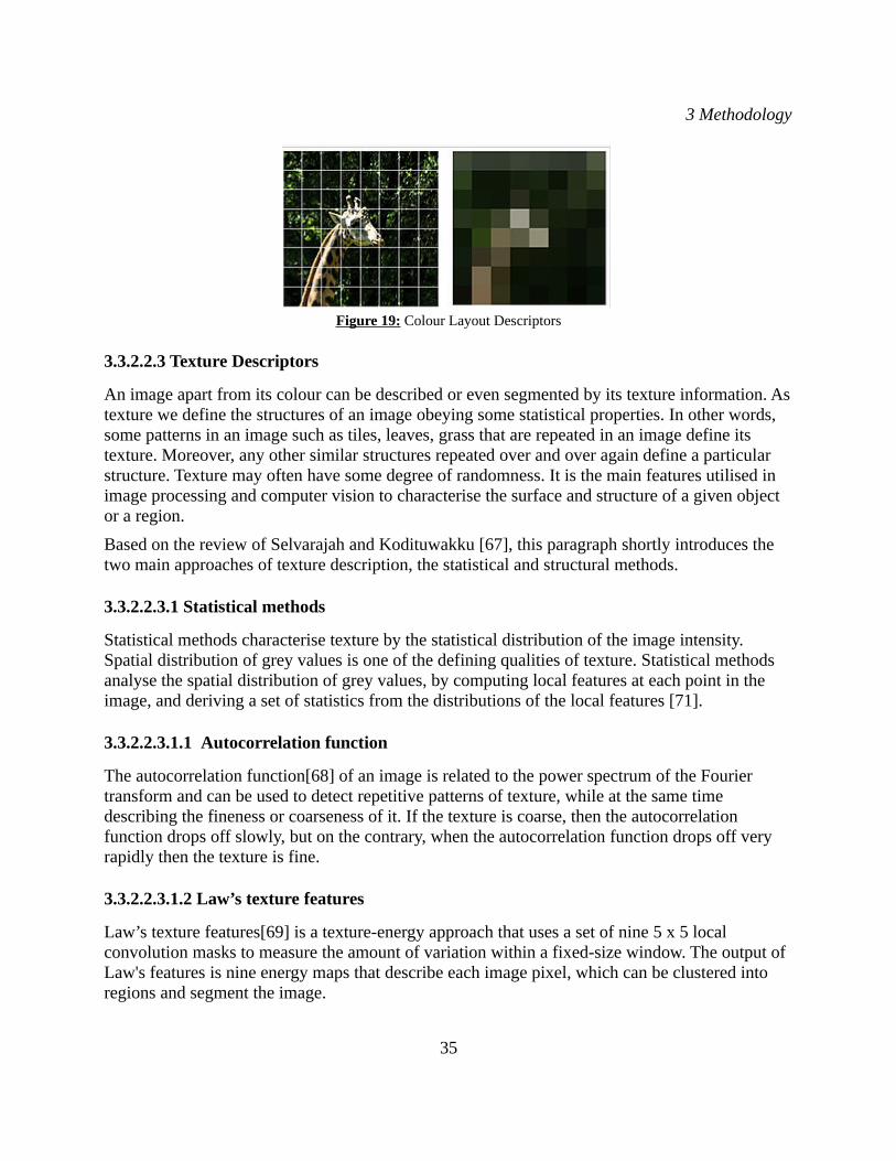
3 Methodology

Figure 19: Colour Layout Descriptors

3.3.2.2.3 Texture Descriptors

An image apart from its colour can be described or even segmented by its texture information. As texture we define the structures of an image obeying some statistical properties. In other words, some patterns in an image such as tiles, leaves, grass that are repeated in an image define its texture. Moreover, any other similar structures repeated over and over again define a particular structure. Texture may often have some degree of randomness. It is the main features utilised in image processing and computer vision to characterise the surface and structure of a given object or a region.

Based on the review of Selvarajah and Kodituwakku [67], this paragraph shortly introduces the two main approaches of texture description, the statistical and structural methods.

3.3.2.2.3.1 Statistical methods

Statistical methods characterise texture by the statistical distribution of the image intensity. Spatial distribution of grey values is one of the defining qualities of texture. Statistical methods analyse the spatial distribution of grey values, by computing local features at each point in the image, and deriving a set of statistics from the distributions of the local features [71].

3.3.2.2.3.1.1 Autocorrelation function

The autocorrelation function[68] of an image is related to the power spectrum of the Fourier transform and can be used to detect repetitive patterns of texture, while at the same time describing the fineness or coarseness of it. If the texture is coarse, then the autocorrelation function drops off slowly, but on the contrary, when the autocorrelation function drops off very rapidly then the texture is fine.

3.3.2.2.3.1.2 Law’s texture features

Law’s texture features[69] is a texture-energy approach that uses a set of nine 5 x 5 local convolution masks to measure the amount of variation within a fixed-size window. The output of Law's features is nine energy maps that describe each image pixel, which can be clustered into regions and segment the image.

35

3 Methodology

3.3.2.2.3.1.3 Run Length Matrices

A grey level run[70] is a set of consecutive, collinear picture points having the same gray level value. The length of the run is the number of picture points in the run. For a given picture, we can compute a grey level run length matrix for runs having any given direction.

3.3.2.2.3.1.4 Gray-level co-occurrence matrix

Haralick et. al.[54] proposed a method that extracts a set of 14 textual features from the co-occurrence matrix, which contains information information about the positions of pixels having similar gray level values. The extracted features contain information about image textural characteristics such as homogeneity, contrast and entropy.

3.3.2.2.3.2 Structural approach

Structural approaches describe texture by identifying structural primitives and their placement rules[67]. The methods presented below offer good results but they have high computational requirements.

3.3.2.2.3.2.1 Wavelet transform

Havlicek and Tay[72] proposed texture detection by means of wavelet transform. After an image being divided into small disjoint blocks, discrete wavelet transform coefficients are computed for each of them. Consequently, the wavelet coefficients are clustered, with each cluster representing a texture segment in the image. Finally, a full dendrogram is constructed giving configurations with a number of clusters ranging from just one super-cluster all the way up to a number of clusters equal to the number of image blocks over which wavelet coefficients were computed.

3.3.2.2.3.2.2 Gabor Transform

Gabor filters have the ability to perform multi-resolution decomposition. The procedure is quite similar to the wavelet transform and consists of the following steps as presented by Hammouda and Jernigan[73]. Firstly, a filter bank tuned to different spatial-frequencies and orientations to cover the spatial-frequency space has to be properly designed. The the image is decomposed into a number of filtered images, the filter defined before is applied to each of them and from its output features are extracted and which they finally get clustered in the feature space. The features can be extracted for example with the magnitude response computation or the smoothed sigmoidal function.

36

3 Methodology

3.3.2.2.4 Shape Descriptors

Shape description constitutes the base of object recognition. As the name may imply, shape descriptors gather information for the shapes extracted from an image. All shape descriptors must respect the following properties[74]. First of all, the property of identifiability, ensures that the shapes found perceptually similar by humans have the same features and different from the others non similar ones. Thereupon, the shape features must be translation, rotation and scale invariant, which means that the values of the features do not change when the shape is translated, rotate, or appears in a bigger scale. In addition to that, the extracted features must be as invariant as possible with affine transforms. Moreover, the features must be noise and occlusion resistant, meaning that the noise included in the shape must not affect the descriptor, as well as given that some parts of the shape are hidden by other objects, the feature of the remaining must remain unchanged. Finally, any shape descriptor must hold the property of reliability and statistical independence. Reliability means that as long as we deal with the same pattern, the extracted features must remain unchanged. Statistical independence guaranteed that two features are statistically independent.

There are many approaches for shape feature extraction an overview of which is shown in Figure[20]. A broad classification of the shape descriptors is briefly described in the following paragraphs, following the same pattern as in [74].

Figure 20: An overview of shape description techniques

37

3 Methodology

3.3.2.2.4.1 One-dimensional function for shape representation

One-dimensional functions used for shape representation are also known as shape signatures[75][76], capturing the perceptual feature of the shape they represent[77]. They may describe a shape all alone or used as a preprocessing to other feature extraction algorithms such as, Fourier descriptors, wavelet description. However, shape signatures are sensitive to noise, and slight changes in the boundary can cause large errors in matching[74]. One-dimensional functions are among others complex coordinates, centroid distance function, tangent angle (turning angles), curvature function, area function, triangle-area representation and chord length function are the commonly used shape signatures.

3.3.2.2.4.2 Polygonal Approximation

Polygonal approximation is an approach of shape representation that overcomes minor variations along the edges of the object represented and capture the overall shape. This is useful because it reduces the effects of discrete pixelisation of the contour[74]. In general, there are two methods to realise it. One is merging, the other is splitting. Among merging methods are the distance threshold method, the tunnelling method and polygon evolution.

3.3.2.2.4.3 Spatial interrelation features

Spatial interrelation features describe the region or the contour of shapes by examining the relations between their pixels or curves[74]. The representation is done by calculating their geometric features: length, curvature, relative orientation and location, area, distance and so on. Spatial interrelation features are adaptive grid resolution, bounding box, convex hull, chain code, smooth curve decomposition, symbolic representation based on the axis of least inertia, beam angle statistics, shape matrix, shape context, chord distribution and shock graphs.

3.3.2.2.4.4 Scale-space methods

Scale space approaches handle shape structure at different scales. In scale space theory a curve is gradually simplified up to point that very small structures vanish as the scaling parameter increases and therefore it is possible to separate small details from relevant shape properties. Two scale-space approaches are curvature scale-space (CSS) and intersection points map (IPM).

3.3.2.2.4.5 Shape transform domain

A shape can also be described by its conversion to the frequency domain. The frequency representation methods can be used in describing a single object or the whole image. The shape feature can be represented by either all the coefficients or partial coefficients of its transform. Some descriptors that fall into this category are Fourier Descriptors, Wavelet Transform, angular radial Transform, shape signature harmonic embedding, R-Transform and shapelet Descriptor.

38

3 Methodology

3.3.2.2.4.6 Moments

Image moments describe a shape by means of its statistical properties the so called moments. This concept is issued from the concept of moments in mechanics where mass repartition of objects are observed[74]. Different moments can be calculated for the boundary of the shape, known as boundary moments or for its region and therefore called region moments. Some common region moments methods are invariant moments, algebraic moment invariants, Zernike moments and radial Chebyshev moments.

3.3.2.2.4.6.1 Invariant moments: Hu Moments

Hu moments[78] are seven moments invariants. Hu moments are invariant to translation changes, scale changes and rotation changes. This makes them a powerful descriptor because it describes a shape despite of its location, size, and rotation.

3.3.2.2.4.6.1.1 Hu Moments OpenCV implementation

Hu moments is a very powerful shape descriptor, and since it consists of seven values it makes the retrieval procedure easier since the feature vector formed is small. The Hu moments are translation, rotation and scaling invariant and regarding the nature of the images, this shape descriptor has been considered one of the best options.

More specifically, the implementation of Hu Moments as offered by OpenCV[197] has been used to in order to compute the Hu Moments that form the feature vector of each image segment, as segmented by the graph-based segmentation algorithm of Felzenszwalb and Huttenlocher(Paragraph 3.2.2.1.9.1).

39

3 Methodology

3.3.2.3 Similarity Measures

Having already discussed several segmentation techniques and description methods in order to represent the segmented image regions in a way that can be easily and fast compared to other segmented regions, it is necessary to discuss so similarity metrics that can be used during the comparison step. The similarity measures can be distinguished in distance-based, feature-based and probabilistic similarity measures[79]. In the next paragraphs some distance-based similarity measures are briefly presented, since the descriptors that are chosen in the current project consist of numerical data.

3.3.2.3.1 Manhattan distance

The distance between two points is the sum of the absolute differences of their coordinates[Formula 3.1]. The Manhattan distance[Figure 21] depends on the choice on the rotation of the coordinate system, but does not depend on the translation of the coordinate system or its reflection with respect to a coordinate axis.

Manhattan Distance=∣x1−x2∣+∣y1− y2∣ (3.1)

Figure 21: left: Manhattan distance, right: Euclidean distance.

3.3.2.3.2 Euclidean distance

The source of Euclidean Distance[Figure 21 right] is the Pythagorean Theorem. Deriving the Euclidean distance between two data points involves computing the square root of the sum of the squares of the differences between corresponding values.

Euclidean Distance=√∑i=1

n∣x i− y i

2∣ (3.2)

3.3.2.3.3 Euclidean Squared Distance

The Euclidean Squared distance metric[Formula 3.3] uses the same equation as the Euclidean distance metric, but does not take the square root. As a result, the Euclidean Squared distance metric is faster than clustering with the regular Euclidean distance.

Euclidean Squared Distance=∑i=1

n∣xi− y i

2∣ (3.3)

40

3 Methodology

3.3.2.3.4 Minkowski Distance

The generalisation of Manhattan Distance and Euclidean Distance is called Minkowski distance[Formula 3.4].

Minkowski Distance(i , j)=(∣xi1− y j1∣q+∣xi2− y j2∣

q+...+∣x ip− y jp∣

q)

1q (3.4), where i, j are the two

different data points to be compared, p the identifier of the variable and q the order of Minkowski metric.

3.3.2.3.5 Canberra Distance

The Canberra metric[Formula 3.5] is a weighted version of the Manhattan distance, which itself is a special form of the Minkowski distance. The distinction is that the absolute difference between the variables of the two objects is divided by the sum of the absolute variable values prior to summing.

Canberra Distance( p ,q )=∑i=1

n ∣pi−qi∣∣pi∣+∣qi∣

(3.5) where pi and qi are vectors.

3.3.2.3.6 Chebyshev distance/Chessboard Distance

Chebyshev distance[Formula 3.6] is a metric defined on a vector space where the distance between two vectors is the greatest of their differences along any coordinate dimension.

d∞( X ,Y )=limq→∞ (∑

i=1

n

∣x i− yi∣q)

1q =max (∣x1− y1∣,∣x2− y2∣,… ,∣xn− y n∣) (3.6)

3.3.2.3.7 Cosine Distance

The cosine similarity[Formula 3.7] between two vectors is a measure that calculates the cosine of the angle between them. This metric is a measurement of orientation and not magnitude, it can be seen as a comparison between vectors on a normalised space because the magnitude is not taken into account but the angle them. The Figure[22] shows three sample cases of cosine scores, with (a) corresponding to similar scores, while (b) are unrelated and in (c) opposite.

Cosine similarity (x , y )=cos (θ)=x∗y

∣x∣∗∣y∣(3.7)

41

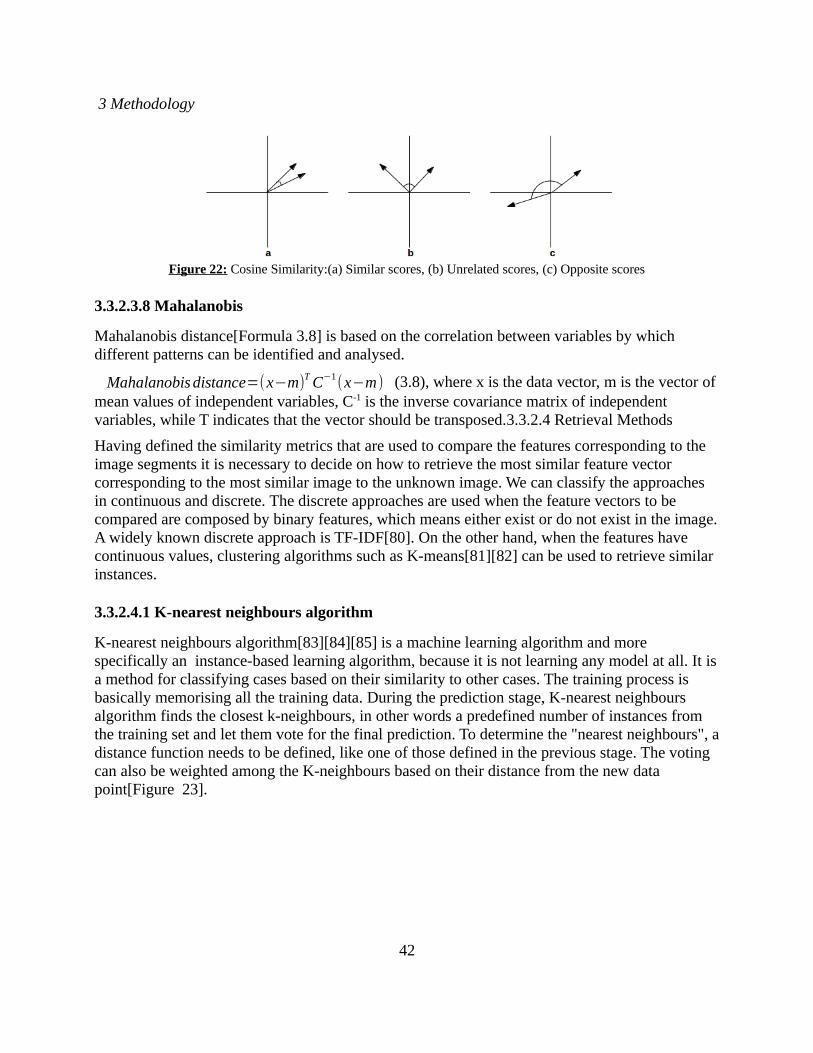
3 Methodology

Figure 22: Cosine Similarity:(a) Similar scores, (b) Unrelated scores, (c) Opposite scores

3.3.2.3.8 Mahalanobis

Mahalanobis distance[Formula 3.8] is based on the correlation between variables by which different patterns can be identified and analysed.

Mahalanobis distance=(x−m)T C−1

(x−m) (3.8), where x is the data vector, m is the vector of mean values of independent variables, C-1 is the inverse covariance matrix of independent variables, while T indicates that the vector should be transposed.3.3.2.4 Retrieval Methods

Having defined the similarity metrics that are used to compare the features corresponding to the image segments it is necessary to decide on how to retrieve the most similar feature vector corresponding to the most similar image to the unknown image. We can classify the approaches in continuous and discrete. The discrete approaches are used when the feature vectors to be compared are composed by binary features, which means either exist or do not exist in the image. A widely known discrete approach is TF-IDF[80]. On the other hand, when the features have continuous values, clustering algorithms such as K-means[81][82] can be used to retrieve similar instances.

3.3.2.4.1 K-nearest neighbours algorithm

K-nearest neighbours algorithm[83][84][85] is a machine learning algorithm and more specifically an instance-based learning algorithm, because it is not learning any model at all. It is a method for classifying cases based on their similarity to other cases. The training process is basically memorising all the training data. During the prediction stage, K-nearest neighbours algorithm finds the closest k-neighbours, in other words a predefined number of instances from the training set and let them vote for the final prediction. To determine the "nearest neighbours", a distance function needs to be defined, like one of those defined in the previous stage. The voting can also be weighted among the K-neighbours based on their distance from the new data point[Figure 23].

42

3 Methodology

Figure 23: Example of k-neighbours classification; 3 training instances vote for a query instance.

For the needs of this master thesis the scikit-learn implementation of k-nearest neighbours was chosen. The distance measuring function as default metric is Minkowski, and with p=2 is equivalent to the standard Euclidean metric[193].

43

3 Methodology

3.3.3 Content-based Image Retrieval System - Proposed method

As mentioned before, the first part of the system is a Content-based Image Retrieval system that searches for images with similar visual content. During the training stage, the images used as training set, are segmented by the graph-based segmentation algorithm of Felzenszwalb and Huttenlocher(Paragraph 3.2.2.1.9.1). All images before the segmentation are converted to thumbnails, in order to reduce the information content and therefore the noise in the image, while still capturing the most important structures in them.

Each segmented area, which is assumed to correspond to an object has to be represented by a featured vector which is easily comparable. Since the training images are not synthetic and therefore quite noisy the extracted features used for the representation feature vector of each region come from the shape of the extracted region, disregarding other features like texture or colour. Thus, each segmented region is represented by a feature vector of Hu moments(Paragraph 3.2.2.2.4.6.1), which are translation, rotation and scale invariant. Finally, all of the feature vectors corresponding to the image segments train a k-nearest neighbour classifier.

When an unseen or query image is given to the system, in order to be summarised, it follows the same procedure as the training images. In other words, a form of the image as a thumbnail is segmented by Felzenszwalb and Huttenlocher's algorithm and then Hu moments are computed for each of its segmented regions. The feature vectors corresponding to each image are mapped to the previously trained classifier and for each feature vector the name of the image corresponding to the most similar image segment is retrieved[Figure 24].

Since the number of the retrieved images is relevant to the number of segments in an image, it may be a very big number. It is obvious too, that if an image is segmented to many regions not all of them are related to the objects or segments in the image that capture the human action and therefore a selection process is followed. The retrieved images are sorted according to their similarity scores in an ascending order and the 26 first images(those with the lowest similarity score, which in other words mean the less amount of differences in the feature vectors and consequently more similar image segments) are chosen for the next selection step. The number was empirically tuned after experiments. The retrieved images have a name that classifies them to one of the four categories consisting the training set. The images are then clustered according to the action they are tagged with, revealed from their name and the set of images corresponding to the class with the lowest frequency is retrieved as similar.

The Content-based Image Retrieval, given a query image returns a set of similar images. Each of the retrieved images are annotated with a short summary. Those summaries are consequently processed in order to extract the common information, that will be used in order to produce the summary for the query image.

44

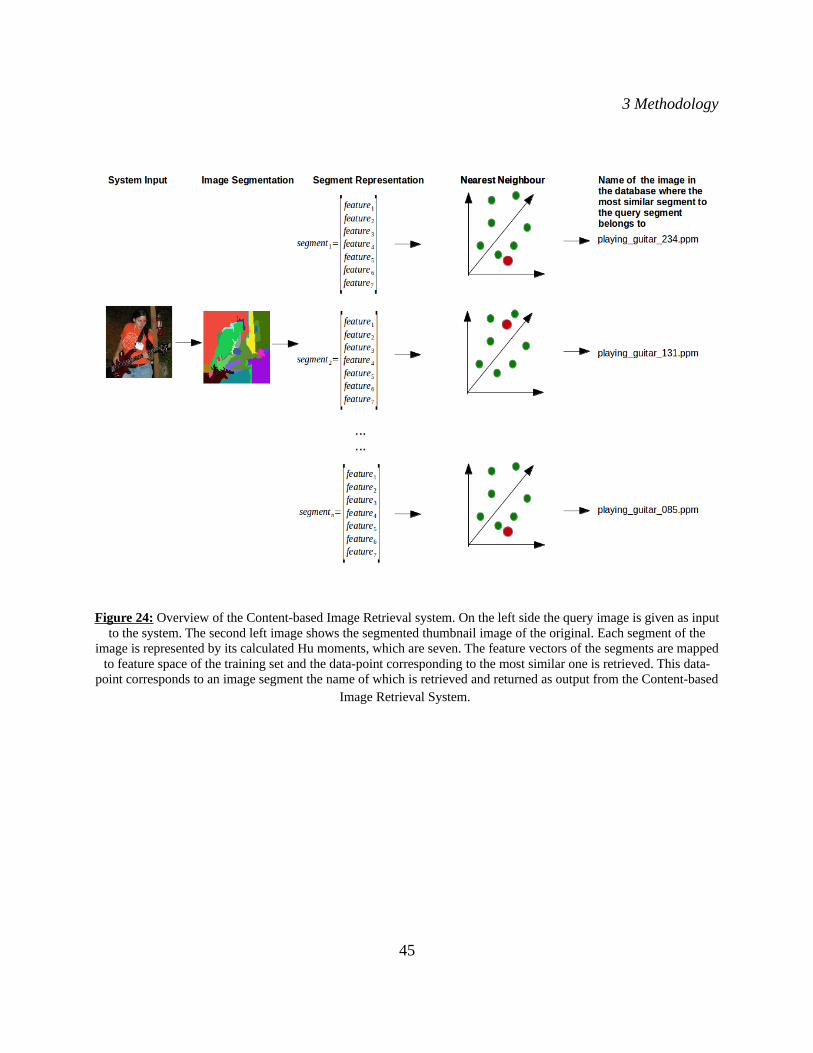
3 Methodology

Figure 24: Overview of the Content-based Image Retrieval system. On the left side the query image is given as input to the system. The second left image shows the segmented thumbnail image of the original. Each segment of the

image is represented by its calculated Hu moments, which are seven. The feature vectors of the segments are mapped to feature space of the training set and the data-point corresponding to the most similar one is retrieved. This data-

point corresponds to an image segment the name of which is retrieved and returned as output from the Content-based Image Retrieval System.

45

3 Methodology

3.4 Natural Language Processing This section starts with an overview in Computational Linguistics and Natural Language Processing. It continues with a focus with a review Syntactical Parsing and Knowledge Representation Systems. Finally, the section closes with the proposed Natural Language Processing system as it was developed for the needs of the current project.

3.4.1 Overview of Computational Linguistics & Natural Language Processing

Computational Linguistics and Natural Language Processing are interchangeable terms for the automatic processing of human language. However, Computational linguistics is a scientific discipline that studies linguistic processes from a computational perspective, while Natural Language Processing is an engineering discipline aiming in the development of useful applications of natural language interest[86].

The counterparts of the psycho-linguistic terms Language Production and Language Comprehension[Figure 25] in Natural Language Processing are Natural Language Understanding and Natural Language Generation. Therefore the goal of Computational Linguistics and Natural Language Processing is to simulate the human communication which consists of conveying meanings, the concepts of the world with the use of words, while processing language as a form of auditory input and map it back to the concepts they are meant with the use of the words.

Figure 25: Language Production versus Language Comprehension

In linguistics, there are six different levels of study[87], phonetics which corresponds to the study of single phones existing in human languages, phonology which studies the combinations of phones in a language, the so called phonemes, morphology, the study of the form of words, syntax, the study of structures between words that form phrases and sentences, semantics which is the study of meaning of words and sentences while the last level is pragmatics, the study of meaning in discourse.

In Computational Linguistics, the before mentioned levels of processing are studied computationally and therefore Speech Processing is the study of the automatic processing of sounds, corresponding to the linguistic phonetics and phonology, a step that is necessary in order

46

3 Methodology

to segment the language input to words(Speech Recognition) or convert words to sounds(Speech Synthesis). In the case of written text this step is replaced by Tokenising, as shown in Figure 26. Lexical analysis[Figure 26] corresponds to morphology, while the rest levels remain the same but treat their aims computationally.

The tasks that belong to morphology are tokenising, stemming and lemmatising and the assignment of categories to words, known as Part-of-speech(POS) Tagging. Tokenising is the processes of finding where the boundaries of a word start and end. There are languages where the writing system makes the task almost trivial because of the use of spaces between the words, like for example English, Hungarian and Greek. The Arabic writing system though or the Chinese, makes this task a lot harder process. Stemming and Lemmatising isolate the stem of the word by removing the parts that produce its inflected form. For instance, playing is the gerund form of the verb to play and therefore the lemma of it is play. Finally, Part-of-speech Tagging checks if a given word in a sentence is a verb, a noun, an adjective and so on.

Syntactic analysis is the study of structural relationships between the words in a sentence. The syntax of a language is described by means of a grammar. In Computational Linguistics there are two ways of syntactical analysis, shallow parsing or chunking and full parsing. Shallow parsing organises the words in a sentence into chunks. It is a partial parsing in order to avoid the disadvantages of full parsers in terms of their high demands. On the other hand, parsing finds all the relationships of the words in a sentence mapping them to trees. Parsing is a fundamental in the progress of this project and will be further analysed in the following section.

Figure 26: The stages of processing in analysis in Natural Language Processing[87]

Syntactic analysis is independent to the meanings of the words. Semantic analysis assigns meanings to words. We can divide semantic analysis into two broad categories, lexical semantics

47

3 Methodology

and compositional semantics. Lexical semantics studies the meaning of individual words, while computational semantics construct the meaning depending on syntax. In other words, compositional semantics study how the meaning of individual units combine to form the meaning of larger units. On the other hand, part of lexical semantics is Word Sense Disambiguation(WSD) which is defined by Jurafsky & Martin[88] as the process of choosing the right sense for a word in context of other words also called word sense tagging by analogy to part-of-speech tagging. Because of the importance of lexical semantics and Word Sense Disambiguation to the current project, they will be further discussed in the following sections.

The next processing level as shown in Figure 26, is the Discourse analysis. Discourse analysis explores the structure of the language while exceeding the clause limits. Anaphora Resolution and Co-reference Resolution belong to the Discourse analysis level. Anaphora Resolution as defined by Mitkov[89] searches for the antecedent of an anaphor(e.g. pronoun or noun referring to a previously mentioned item). On the contrary, the goal of Co-reference Resolution is to find the mentions in text that refer to the same real-world entity[90].

Last but not least, Dan Jurafsky[91] mentions about Computational pragmatics that it might be defined as the computational study of the relation between utterances and context. Computational pragmatics is concerned with indexicality, with the relation between utterances and action, with the relation between utterances and discourse, and with the relationship between utterances and the place, time, and environmental context of their being uttered. Bunt and Black[92] point inference as the main concern in both Pragmatics and Computational Pragmatics, which is the process of filling in information that is not present in the utterance at hand. Moreover, Speech act interpretation is also a classic pragmatic problem. Speech acts can be defined as the information extracted from the speech prosody inferring information about the psychological state of the interlocutor, irony, empathy, sympathy, that is not directly expressed by means of words.

Having comparatively explained the steps in Linguistics and Computational Linguistics, it is important to provide an overview of Natural Language Processing. As mentioned before, is usually characterised as an engineering discipline, which builds tools involving language input or language output. Therefore, we can classify its applications into those involving exclusively Natural Language Understanding or Natural Language Generation or a combination of both of them. The current project involves a combination of both of them, since it first searched the common information according to some syntactic criteria and after given the extracted information, it produces a sentence, trying to simulate the way a human would do.

Some very well known Natural Language Understanding areas of research and application are Information Extraction, Sentiment Analysis, Event extraction and role labelling. A typical Language Generation application is the automatic report generation from structured database data, either of number or textual content, while a combination Natural Language Understanding and Generation are Machine Translation, Question Answering and Text Simplification. The common feature of the first applications is that they map from text to some structured meaningful representation, while the second ones combine this structured information to produce a text that embodies the meaning extracted from the previous step. As mentioned already before, the

48

3 Methodology

current project requires both fields and more specifically information extraction, to find the required information and the produce a linguistic output.

3.4.2 Syntax in Language

In the previous, section syntax has been defined as the study of structure in a language. The main linguistic theories can be grouped in three categories. Prescriptive theories study how the people should use the language. Descriptive theories study how people actually do talk. On the other hand, explanatory theories provide a set of universal language principles and language-specific parameters[165]. In the next paragraphs and brief explanation of the constituency theory and dependency theory and their application in syntactical parsing.

3.4.2.1 Constituency Theory

Constituency Theory was introduced by Noam Chomsky and as the name of it reveals, the main relation in syntactical analysis is this of constituency. Phrase-structure grammars are based on constituency, where its groups of words that belong together are called constituents. The component that determines the properties of the constituent is the head, and the constituent can be referred to as a phrase: e.g. noun phrase. The analysis of a sentence in its constituents results in a tree like this in Figure 27.

Figure 27: Representation corresponding to constituency grammar.

3.4.2.2 Dependency Theory

Dependency Parsing has its roots back in the 5ht century BC reflected in Pā ini's Grammar, ṇwhile more recently in 1959, Lucien Tesnière[109][110] revived the theory of dependencies between the words in a clause. More specifically, syntactic structure consists of lexical elements linked by binary asymmetrical relations called dependencies. A dependency relation[Figure 28] holds between a head and a dependent. Alternative terms in the literature are governor and regent for head and modifier for dependent. In dependency theory, the central ideas as expressed by L. Tesnière[109][110] are the terms of valency, arguments and adjuncts. The theory of valency

49

3 Methodology

refers to the number of arguments controlled by a verbal predicate including the subject of the verb, with arguments being defined as the expressions that complete the meaning of a predicate. Arguments should not be confused with adjuncts, that are optional which means that if they are removed or discarded, they do not affect the meaning of the remainder of the sentence. An argument is not an adjunct and an adjunct is not an argument.

Figure 28: Representation corresponding to Dependency Analysis

3.4.2.3 Syntactic Parsing

Nivre[93] defines the syntactic parsing as a structural prediction problem, where an input space X of sentences is mapped to an output space Y of syntactic representations. An input sentence x ∈X should be mapped to a syntactic representation y Y. A syntactic parser is based on a ∈mathematical model M relating the input space X to the output space Y. More specifically, a parsing model M can be seen as an optimisation problem of choosing the best syntactic representation among those produced for the given input.

The following section describes the two main approaches in syntactical parsing or else text parsing as categorised by Joakim Nivre[111] in his work "Two Strategies for Text Parsing".

3.4.2.3.1 Grammar-driven text parsing versus data-driven text parsing

Grammar-driven parsing is inspired by the generative grammars as proposed by Chomsky[112]. Grammar-driven approaches are deductive and make the assumption that any text of a language can be approximated by a formal language as this formal language is defined by a grammar. The problems of these approaches, as figured by Joakim Nivre[93] are the lack of robustness and their weakness in dealing with ambiguity. In other words, they are not able to analyse any input sentence. In order to deal with the inefficiency of robustness, the constraints of the grammar can be either relaxed, or kept and recover as many structures as possible from the well-formed fragments of the sentence, a method also known as partial parsing. On the other issue of disambiguation, the assignment of more than one analyses to a given input, the solution is either the use of specialised grammars for different domains of text or the choice of the appropriate parsing methodology or the integration of statistical information in order to rank the returned analyses and select the best one among them. It should be mentioned though, that the required

50

3 Methodology

adjustments, in order to improve the robustness and the disambiguation of the gramman-driven approaches compromise efficiency by causing a combinatorial explosion.

On the other hand data-driven parsing does not require a given formal grammar and depend on inductive inference from a representative language sample. In the data-driven approaches, the robustness problem is avoided by a kind of superset approximation, meaning that any sentence can be assigned an analysis but not the opposite. In terms of the disambiguation problem, which might more serious than in the grammar-based approaches, the data-driven approaches can be solved by the fact that the inductive inference scheme provides a mechanism for disambiguation, either by associating a score with each analysis, intended to reflect some optimality criterion, or by implicitly maximising this criterion in a deterministic selection. Finally, the data-driven approaches prove to be superior to the grammar-driven approaches, however they output representations are less adequate.

In order to balance the advantages and the disadvantages of the grammar-driven and the data-driven approaches, there have been attempts to combine both of them, such as broad-coverage parsers based on the PCFG model[113] or on linguistically motivated frameworks such as LFG[114].

3.4.2.3.2 Phrase structure parsing

Constituency grammars are also called phrase structure grammars. The next section is devoted in phrase structure parsing, offering an overview of the development in this research field as surveyed by Joakim Nivre. The section starts the simple context-free grammars and then continues by discussing several generative and discriminative approaches. The classification of the approaches follows the pattern of Nivre.

3.4.2.3.2.1 Context-free Grammars & Chomsky

A context-free grammar consists of a set of terminal symbols, which in syntactical parsing correspond to words, a set of non-terminal symbols, that corresponds to the name nodes that can be used to form the parsing tree structure we want our system to output, a start symbol and a set of rules.

Specific Chomskyan theories changed regularly throughout the time, but the core of Chomsky's work treats syntax as a cognitive reality and supports the existence of a biological universal grammar. The formalism of context-free grammars was developed in 50s by Noam Chomsky and also their classification as a special type of formal grammar called as phrase-structure grammars[166], which corresponds to the already mentioned constituency grammar. According to the generative grammar framework, the syntax of natural language is described by context-free rules combined with transformation rules. The algorithms typically used in order to parse CFGs include dynamic programming such as Earley parser[96] and the bottom-up parser Cocke–Younger–Kasami (CYK) algorithm[95].

51

3 Methodology

3.4.2.3.2.2 Generative parsing models

Generative parsing models define the joint probability of the input sentence and the output syntax tree. The advantages of generative models are the facts that they offer closed form solutions and that the related probabilities can be computed through conditionalisation and marginalisation. On the other hand, they require rigid independence assumptions, and training a generative statistical parser maximises the joint probability of inputs and outputs in the training set, which is only indirectly related to the goal of parsing[93].

3.4.2.3.2.2.1 Parsing Probabilistic Context-free Grammars

A Probabilistic context-free grammar(PCFG) is a simple extension of a Context-free grammar in which every production rule is associated with a probability[94]. PCFGs are the most important generative formal models in syntactic parsing, and have been the core for further developments, also mainly used in speech recognition and statistical machine translation, since they can be used to model the probability distribution of a string language.

A PCFG model according to the formal definition of Nivre[93], computes, given a specific grammar G and an input sentence x, the set of candidate representations while scoring each candidate by the probability P(y), as defined by the grammar. For the candidate representation, a CFG model is used and for the scoring many of the standard algorithms CFG parsing have a straightforward extension, which is a dynamic programming algorithm, that computes the probabilities of parse trees in the same process, like for instance CYK algorithm[95], Earley's algorithm[96], and the algorithm for bi-lexical context-free grammars[97]. The PCFG models can be either provided with a context-free grammar or learn a grammar from a sample of sentences with the correct parse trees for each of them(e.g. Charniak[98]), called as a treebank grammar.

A PCFG from a treebank is not likely to give the best possible parsing accuracy, therefore advanced PCFG models integrate techniques for transforming a plain treebank grammar to a grammar that is better suited for parsing. A simple way to improve the classical PCFG is parent annotation as proposed by Johnson[99], which consists in adding to the non-terminals of each node of the parsing tree, the non-terminal of the parent node . Another technique, called lexicalisation enhances similarly to the parent annotation, each non-terminal symbol with a terminal symbol. For example, in head-lexicalised PCFGs[100][101][102] the terminal equals to the same lexical head as the one of the parent category , with the heads being extracted with a set of percolation rules. On the other hand, Markovisation, as defined by Nivre, is a technique for splitting n-ary grammar rules into sets of simpler rules that generate one child at a time, conditioned on a limited number of siblings, thereby making the grammar more robust to missing rules(e.g. Stanford unlexicalised parser[157]). Finally, Petrov et al. [103] extended the markovisation by replacing each non-terminal observed in the treebank by a set of categories for each non-terminal, defined by latent variables. In this case, it is crucial to find the right level of granularity for a given category which can be accomplished with the use of an iterative split-merge strategy.

52

3 Methodology

3.4.2.3.2.3 Discriminative Models

Discriminative parsing model only make use of the conditional probability of a candidate syntax tree given an input sentence ignoring the joint probability. Therefore, the discriminative models can define features over the input and in contrast to generative models they have no rigid independence assumptions and can model the problem more directly. However, discriminative training methods normally require the use of numerical optimisation techniques[93].

Discriminative models are divided in two categories, the conditional and the purely discriminative models. The conditional models compute the conditional distribution of outputs given inputs, while the purely discriminative models optimise the mapping from inputs to outputs without modelling a conditional distribution.

3.4.2.3.2.3.1 Local

Local discriminative models are conditional models, that assume that a global solution can be achieved by taking local optimal decisions. Local models[104][105][106] have the advantage that can also be trained very efficiently using logistic regression or similar methods and perform in linear time. However, their accuracy is not better than best-performing generative models and global discriminative models. Moreover, these parsers use heuristic search algorithms and as a result it cannot be guaranteed that the most probably parse tree will be found for a given sentence.

3.4.2.3.2.3.2 Global

Global discriminative models maintain a conditional model over the entire output structure given an input. However, in order to make learning tractable computationally, the feature model needs to factor into reasonably local, non-overlapping structures, so that dynamic programming can be used. The main disadvantage of global models is that the features are only local. Global discriminative models[107] have been used as an alternative to the generative PCFG model.

3.4.2.3.2.3.3 Re-ranking

Re-ranking parsers[108] are the answer to the complexity of conditional models, improving the parsing accuracy. The global discriminative model is used to re-rank the n top candidates already ranked by a base parser, which is often a generative PCFG parser and because the set of candidate parses is small there is no need for dynamic programming and therefore global features are enabled without imposing any particular factorisation.

3.4.2.3.3 Dependency Parsing

A dependency parser analyses syntactic structures by identifying dependency relations between the words. Some of the advantages of dependency parsing as reviewed by Joakim Nivre are the fact that dependency relations are close to semantic relations, which facilitates semantic interpretation and the fact that dependency representations are more constrained, which facilitates

53

3 Methodology

parsing, while they are more suitable for languages with free or flexible word order. On the other hand, dependency representations are less expressive and less well understood formally and computationally.

In a dependency tree, a sentence is analysed by connecting words by binary asymmetrical relations, which are categorised according to the functional role of the dependent word.

According to the formal definition of dependency parsing as given by Joakim Nivre, a dependency tree for a given sentence can be defined as a labelled directed graph, which firstly must have a dummy root that has not incoming arc, secondly is weakly connected, and finally for every of its nodes there is at most one incoming arc. Depending on the approach, the requirement of projectivity may or may not be fulfilled. In other words, for every arc in the tree, there can be a directed path from the head of the arc to all words occurring between the head and the dependent.

In contrast to the phrase structure parsing, the parsing problem for a dependency parser is more constrained since it consists of finding the optimal dependency tree given an input sentence, by assigning a syntactic head and a label to every node corresponding to a word, in a way that the final graph is a tree with a dummy root. This is a lot simpler in the sense that the nodes are already given with only the arcs missing, while in phrase structure parsing the nodes, their labels and the arcs are all sought. Moreover, there are no part-of-speech tags in the tree representation of dependency parsing, while in most of the cases they are assumed to be provided with the input sentence and are important features that determine the final output. Last but not least, dependency parsers tend to use purely discriminative models instead of probability models.

3.4.2.3.3.1 Graph-based parsing

As the name of the graph-based parsing infers, the parsing of a sentence input is approached with the use of graphs. According to the factorisation of a scoring function the graph-based models can be distinguished in first-order models such as arc-factored models that will be described later and higher-order models. The first-order models behave similar to imposing independence assumption in PCFGs, as already mentioned before.

3.4.2.3.3.1.1 Projective Parsing versus Non projective Parsing

First order projective trees can be decoded with Eisner's algorithm[116][117] and with some adaptations Eisner's algorithm higher-order models can also be decoded. Such adaptation in Eisner's algorithm for the second-order sibling(nodes sharing the same head) model has been proposed by McDonald & Pereira[120].

In case of non-projective models things get more complicated. Graph-theoretic algorithms like Chu-Liu-Edmonds[118][119] can be used for efficient first-order, non-projective dependency parsing. However, these methods cannot be generalised to cover also higher-order models. It has been shown that non-projective parsing with higher-order models improves the parsing accuracy while at the same time being NP hard[121]. For this reason approximation approaches have been used such as in McDonald & Pereira's work[120] where the first step is to find the best projective

54

3 Methodology

tree using Eisner's algorithm and the second step is to iteratively substitute arcs in the tree as long as the score of the tree improves. Other approaches that approximate higher-order non-projective dependency parsing are based on general optimisation techniques such as integer linear programming [122][123], belief propagation[125] and dual decomposition[124].

3.4.2.3.3.1.2 Arc-Factored Models

A widely used graph-based model for dependency parsing is the arc-factored or edge-factored model, where the score of a dependency tree decomposes into the scores of individual arcs. The generative component of these models maps each sentence to the set of all spanning trees for the node set of the given sentence . Thereafter, the evaluative component ranks all the candidate trees according to their arc-factored score and returns the one with the highest score. The score is computed with a weighting feature function that ranks each arc according to the input features. The weights of an arc-factored model can be learnt in many ways, but the most popular approach is to use an online learning algorithm that parses one sentence at a time and updates the weights after each training example with the goal of minimising the number of errors on the training corpus, as for example a simple perceptron[115]. In order to find the highest scoring dependency tree for a given sentence a decoding algorithm is needed such as Eisner's algorithm[116][117] in case we are searching for a projective spanning tree or with standard graph theory algorithms for extracted the maximum spanning tree(e.g. Chu-Liu-Edmonds algorithm[118][119])

3.4.2.3.3.2 Transition-based parsing

As defined by Nivre[126], transition-based models for dependency parsing use a factorisation defined in terms of a transition system, or abstract state machine. Each transition-based model consists of a set of configurations, a set of transitions, an initialisation function and a set of terminal configurations. A configuration for a sentence consists of a list of nodes, known as the stack, a list of nodes, known as the buffer, and a set of dependency arcs. Algorithms are defined in terms of a transition system, consisting of a set of configurations and a set of transitions between configurations. Deterministic parsing is implemented as greedy best-first search through the transition system.

3.4.2.3.3.2.1 Arc-standard system projective parsing

Arc-standard systems are suitable for projective dependency parsing. In such systems, the initial configuration for a sentence is a configuration where the stack contains the artificial root node, the buffer contains all the nodes corresponding to the real words of the sentence and where the arc set is empty. A terminal configuration is any configuration where the stack again contains only the artificial root node and where the buffer is empty. Whatever arcs have been accumulated in the arc set at that point defines the parse for that transition sequence. There are three types of transitions for getting from one configuration to the next. The "shift" transition removes the first node in the buffer and pushes it on top of the stack. The "left-arc" transition adds a dependency arc to the arc set between the first and the second nodes from the top of the stack, while it also

55

3 Methodology

pops the stack twice and then pushes the first node back on to the stack so that only the head node remains on the stack after the transition but ensuring at the same time that there are no arcs added going into the artificial root node. Finally, "right-arc" adds a dependency arc to the arc set between the second and the first node from the top of the stack, while it also pops the stack once so that only the head node remains on the stack after the transition.

The arc-standard system considered so far builds a dependency tree bottom-up, meaning that a dependency arc can only be added between two nodes if the dependent node has already found all its dependants. As a consequence, it is often necessary to postpone the attachment of right dependants which turns them to non-deterministic models.

3.4.2.3.3.2.2 Arc-eager system parsing

Arc-eager systems avoid the non-determinism problem of arc-standard systems. Those systems always adds an arc at the earliest possible opportunity and which therefore builds parts of the tree top-down instead of bottom-up. They have the same initialisation function as the arc- standard system, but the set of terminal configurations is different because the arc-eager system terminates as soon as the buffer is empty. The transitions of arc-eager systems are; "shift" transition as introduced before in arc-standard systems , "left-arc" transition, which is analogous to "left-arc" in the arc-standard system except that the new arc combines one node from the stack and one node from the buffer instead of the two top nodes on the stack, "right-arc" transition, which however is different from "right-arc" in the arc-standard system not only because the new arc combines one node from the stack and one node from the buffer but also because both nodes are retained in the new configuration, and finally "reduce"transition, that removes the node on top of the stack subject to the condition that it has already been assigned a head in the dependency structure.

3.4.2.3.3.2.3 Non-Projective Parsing

In the case of non-projective parsing Attardi[127] proposed an extension to the arc-standard system with additional transitions for adding arcs between nodes that are not adjacent on the stack. Another approach proposed by Nivre[128] relies on the notion of online reordering, where instead of adding arcs between nodes that are not adjacent on the stack the parser is allowed to reorder the nodes so that nodes that should be linked by an arc are always adjacent this happens by using a transition called "swap" to reorder nodes by moving the second node on the stack back to the buffer except for the case where the node is the root node or the nodes have been already swapped. Finally, a last technique called pseudo-projective parsing[129]. that keeps the parsing process strictly projective, thus preserving linear time complexity, but nevertheless allows the recovery of a subset of the non-projective dependencies in post-processing.

3.4.2.3.4 State-of-the-art parsers

In the previous paragraphs. the two main kinds of syntactical parsing were briefly introduced, corresponding to the main two linguistic approaches, the Chomskyan[166] about constituency

56

3 Methodology

theory and dependency theory as introduced by Tesnière[109][110]. For each of them the most important methods have been discussed based on Nivre's review[93]. This section will briefly describe two state-of-the-art parsers, MaltParser and Stanford parser.

3.4.2.3.4.1 MaltParser

As far as dependency parsing is concerned, MaltParser[163] is a data driven state-of-the-art parser that constructs a parser given a treebank. MaltParser is an implementation of inductive dependency parsing [164], where inductive machine learning is used to guide the parser at non-deterministic choice points. As defined by Nivre[126], the components of transition-based parsing are deterministic parsing algorithms for constructing labelled dependency graphs, history-based models for predicting the next transition, discriminative learning to map histories to transitions. There is an open source implementation of MaltParser available online[167].

3.4.2.3.4.2 Stanford Dependencies and Stanford Parser

Stanford Parser is another state-of-the-art parser and its implementation is also an open source[156]. The implementation package includes an unlexicalised PCFG[157], a lexicalised dependency parser and a factored model[159], where the estimates of dependencies[158], and an unlexicalised PCFG are jointly optimised to give a lexicalised PCFG treebank parser. Moreover, there are included grammars for various languages(e.g. German[160], Chinese[161], Arabic[162]) for use with these parsers. The Stanford parser output is a constituency tree and a dependency tree either in its typical form of a structure with either collapsed dependencies or basic dependencies. In comparison to a typical dependency parser, Stanford parser is not a dependency parser as this kind of parsers were described before. The extracted dependencies of the Stanford parser come from a phrase structure parse.

Stanford Dependencies[168] are approximately 50 grammatical relations , that can take either collapsed[Figure 29] or basic form[Figure 30]. In the collapsed representation, dependencies involving prepositions, conjuncts, as well as information about the referent of relative clauses are collapsed to get direct dependencies between content words.

57

3 Methodology

Figure 29: Stanford collapsed dependencies

Figure 30: Stanford dependencies

58

3 Methodology

3.4.3 Lexical Semantics and Word Sense Disambiguation

Navigli[130] mentions that Word Sense Disambiguation is an AI-complete problem. AI-complete or AI-hard is a task of difficulty equivalent to the central problem of Artificial Intelligence which is computational simulation of the human intelligence. There have been several approaches to deal with Word Sense Disambiguation, that can be classified in supervised, unsupervised and knowledge-based[130]. The supervised approaches require labelled corpora, while the unsupervised work with unlabelled corpora. On the other hand, knowledge-based approaches require external language resources, some of which are presented in the next paragraph.

3.4.3.1 Knowledge Organisation Systems

Knowledge Organisation Systems are of crucial importance for several semantic tasks in Natural Language Processing, since they are systems that organise parts of the world knowledge. Knowledge is a fundamental key factor in Word Sense Disambiguation. Knowledge sources provide data which are essential to associate senses with words[130]. They can have several forms according to the kind of information they offer and we can distinguish them to structured and unstructured. Structured knowledge systems are taxonomies, thesauri, machine-readable dictionaries and ontologies. Unstructured resources can be corpora of texts labelled with word senses(e.g. SemCor [133], MultiSemCor [134], DSO corpus [135]), unlabelled(e.g. Brown Corpus[131], British National Corpus (BNC)[132]) or collocation resources(e.g. Web1T corpus [136]).

3.4.3.1.1 Machine-readable dictionaries

Machine-readable dictionaries contain an enormous amount of lexical and semantic knowledge collected together over years of effort by lexicographers[137]. The research in this field has been devoted to devising methods to automatically extract this information from dictionaries.

3.4.3.1.2 Taxonomies

A taxonomy is a hierarchical tree structure starting from the most general thing or concept as a root expanding down to the most specific things or concepts[Figure 31]. Taxonomies consist a form of knowledge organisation having been used in Natural Language Processing in tasks such as checking taxonomic similarity in resolving syntactic and semantic ambiguity[138][139]. Since taxonomies can be an important tool in Word Sense Disambiguation, there have been efforts in the NLP community to development methods that extract taxonomies automatically[140].

59

3 Methodology

Figure 31: A taxonomy of animals.

3.4.3.1.3 Thesauri

A thesaurus is a hierarchical structure that defines a controlled vocabulary, like a taxonomy, it but includes more information than just a name, such as synonyms, an explanation of the category, related categories, and any other possible features. A thesaurus differs from an ontology in the sense that it has weaker semantics, while a thesaurus can represent interesting source for the development of more formal ontologies. The are most widely used thesaurus in the field of WSD is Roget's International Thesaurus[141], while also the Macquarie Thesaurus [142]. Thesauri have been traditionally used in digital libraries to improve precision and recall of information retrieval systems. An example can be shown in Figure 32, where we see three kinds of relations from the item "Germany" to other items such as "Europe". "Germany" is a part of "Europe" and its relation to Europe is broader, unlike to "Berlin" which belongs to "Germany" and its relation is "narrower".

Figure 32: Thesaurus representation; Relations between concepts

3.4.3.1.4 Ontologies

An ontology is usually not restricted to hierarchical relations between categories, but also includes any other kind of relationships between the items. According to the definition of Gruber, an ontology is an explicit specification of conceptualisation, while conceptualisation is an abstract, simplified view of the world that needs to be represented for some purpose[143].

60

3 Methodology

Navigli[130] mentions examples of ontologies, such as SUMO upper ontology[144] and Omega Ontology[145], which is an attempt to conceptualise WordNet.

3.4.3.1.4.1 Lexical Ontologies & Wordnet

A lexical ontology is an ontology of lexicalised concepts. In other words, only concepts that are expressed by words are included in a lexical ontology. WordNet is usually defined as a lexical ontology. The WordNet definition about WordNet itself is "a machine-readable lexical database organised by meanings; developed at Princeton University"[155], while Christiane Fellbaum defines WordNet as a large semantic network interlinking words and groups of words by means of a lexical and conceptual relations represented by labelled arcs[146][Figure 33].

WordNet contains more than 118,000 different word forms and more than 90,000 different word senses[147]. WordNet's building blocks are synonym sets called as "synsets", which are unordered sets of cognitively synonymous words and phrases[146]. The syntactic categories included in it are nouns(entities), verbs(events), adjectives(properties) and adverbs. On the other hand, prepositions, pronouns, and determiners are given no semantic explication in WordNet. As far as inflectional morphology is concerned, is accommodated by the interface to the WordNet database. However, derivational and compound morphology are entered into the database without explicit recognition of morphological relations[147].

The semantic relations in WordNet as sorted by Miller[147] are synonymy, antonymy, hyperonymy, meronymy, troponymy and entailment. With synonymy being a symmetric relation and the basic WordeNet relation, the words are organised in sets of synonyms the before mentioned "synsets" representing the same word senses. Antonymy is another symmetric semantic relation between word forms that have the opposite meaning, which is important for the organisation of the meanings of adjectives and adverbs. Hyperonymy and its inverse hyponymy are transitive relations between "synsets" and since there is usually one hyponym, hyperonymy organises the meaning into a hierarchical structure. Meronymy with its counterpart holonymy, on the other hand, are characterised as semantic relations, that organises the nouns in component parts, substantive parts and member parts. Troponymy has the same function as hyponym, but instead of nouns it concerns verbs. Finally, entailment relations between verbs, is the relation that shows whether a verb can be inferred from another. The Table 3 shows the WordNet relations and the respective category of words that is involved in each relation.

61

3 Methodology

Table 3: Semantic Relations in WordNet

However, as Fellbaum points, WordNet does not contain any syntactic information and therefore can be considered as a composition of four unconnected WordNets, each one corresponding to nouns, verbs, adjectives and adverbs. As a consequence, thematic and semantic roles of nouns functioning as arguments of specific verbs are not encoded . In addition, WordNet's contents are largely derived from its creators' intuitions, since when it started being created there were not many digital corpora available.

Figure 33: An excerpt of the WordNet semantic network

62

3 Methodology

3.4.4 Information Extraction

Information Extraction is the process of automatically extracting structured information from an unstructured source. It is a very broad field, therefore there are several ways to approach a specific Information Extraction problem depending on the type of information we want to extract, the kind of source we want to extract it from, the type of input resources available for extraction, the extraction methods, as well as the kind of output we expect from the system[153].

The type of structure extracted can be among others, entities such as in named-entity recognition (NER) or acronym expansion systems, attributes, relationships and higher-order structures such as lists and tables. Entities are typically noun phrases and are no longer than a few tokens in the unstructured text. The most popular form of entities is named entities like names of persons, locations, and companies(MUC [148][149], ACE [150][151], and CoNLL [152] competitions). Moreover, an Information Extraction system might search for predefined relationships between two or more entities related in a specific way. In addition to that, the attributes of a given entity with the value of an adjective describing the entity, might need to be extracted. Finally, richer structures such as tables, lists and trees of various types of documents might be extracted(e.g. taxonomy or ontology extraction[154]).

As already mentioned, the type of the unstructured source is a factor that influences the Information Extraction System we want to develop. More exactly what is of big importance is that basic unit of granularity on which the extractor is run and the heterogeneity in style and format across unstructured documents. For example, the source can vary from a short string, a sentence and a paragraph to a whole document.

Moreover, the Information Extraction Approach can be influences by the type of input resources available for extraction, as for instance structured databases, labelled unstructured data, or even linguistic tags. An important concern that has a huge impact on the complexity and accuracy of an extractor is how much homogeneity of the document. For example the complexity of extracting information from an html machine generated page is a lot lower than the complexity of processing a semi-structure domain source, or an open-ended source such as the web.

On the hand, the method used for the extraction influences a lot the implementation of the information extractor. For example rule-base and manually coded systems are approached in a different way than trained from examples systems. A hand-coded system requires human experts to define rules or regular expressions or program snippets for performing the extraction. In contrast, learning-based systems require manually labelled structured examples to train machine learning models of extraction. Even in the learning-based systems, domain expertise is needed in identifying and labelling examples that will be representative of the actual deployment setting. The nature of the extraction task and the amount of noise in the unstructured data should be used to decide between a hand-coded and a learning-based system.

Finally, the desired output from the extractor is also an influence factor. In other words, the stage after extracting the desired information, it may be required that the extracted information has to be filled in a database or the extracted information has to be presented in an annotation form on the original text, in the cases where the original unstructured source is required by the user.

63

3 Methodology

3.4.5 Natural Language Processing System - Proposed method

As already described in paragraph 3.3.3, the Content-based Image Retrieval, given a query image returns a set of similar images. Each of the retrieved images is annotated with a short summary(the ones collected during the annotation phase in section 3.2). Those summaries are consequently processed in order to extract the common information, that will be used in order to produce the summary for the query image.

3.4.5.1 Dependency parsing

Each of the sentences corresponding to the retrieved images is parsed by Stanford parser(paragraph 3.4.2.2.4.2) and represented in a dependency graph form[Figure 34], where the nodes are the words with their part of speech tag and the edges are named with Stanford collapsed dependencies. As already described before, Stanford parser is a phrase-structure parser extended with a rule-based post-processing step that extracts dependency graphs and can be used for dependency parsing.

A dependency representation of the sentences has been selected because it is assumed that the verb of the sentence captures the main action depicted in the image, while the subject and the object should correspond to the main subjects and objects in the image. Moreover, the information extraction method selected for this task is graph based and dependency parsing offers a graph labelled with the words of the sentence and edges showing the dependencies organised around the verb. Therefore dependency parsing offers a good base to develop the system further. Particularly, Stanford parser was selected because of the ease offered by its collapsed dependencies. Moreover, for the kind of sentences gathered by the annotation Stanford parser showed empirically very high accuracy results and robustness to the noisy inputs.

3.4.5.2 Graph merging

The next step is a graph merging stage, during which the dependency graphs of the previous steps are joined according to their common nodes and edges to form a bigger graph or graphs. In order to merge a node with another node, they are compared to each other. The nodes are labelled by the name of the word, as well as the Part-of-Speech tag. If the tags are the same then the names of the nodes are compared as simple strings. If they are identical, they are merged and a weight corresponding to the nodes is update to show the frequency of the word. The same procedure is followed for the edges. Edges that share the same label and connect the same nodes and are also merged and a weight is updated according to their frequencies.

Because of the nature of the text to be processed for this specific task the main hypothesis about the most important information, is that the verb captures the main action depicted in the image and therefore in order to merge the graphs another strategy is also adopted. In this case, the nodes that are the subjects and the objects of the verb are examined for their their semantic similarity. To make this clear, the nodes that are extracted to be as subjects from the parser consist a set, the members of which are compared to each other with the help of WordNet, in order to identify whether they are semantically related. If there is an edge between them like for example

64

3 Methodology

connected by the conjunction "and" they are not checked for semantic similarity since they refer to different entities.

The semantic similarity that is used for node merging exists when the two nodes share a common hypernym. If a common hypernym is found, then they are both replaced by the common hypernym and their dependencies are therefore modified and adjusted to the newly inserted node. For instance, the words "boy" and "man" are substituted by their common hypernym which is "male". It should be highlighted though that the semantic similarity is searched only when the node is a common noun and not in case of proper nouns. The same process is repeated for the direct objects, in order to check if there are any nodes that can be merged by their common hypernym.

Figure 34: Dependency Representation of all the texts corresponding to the similar retrieved images to the query image on the left

In the case of verbs, a lemmatising process is used in order to check for common lemmas between the two words, such as in case of "play" and "playing". If the nodes share the same lemma then they are merged and their dependencies to other nodes are also updated, as well as their weights.

65

3 Methodology

The graph merging phase is completed after the four stages of common string nodes merging, common subject hypernym and common object hypernym merging as well as the same verb lemma merging are carried out.

3.4.5.3 Optimal path extraction

Figure 35: Cut of the merged graph from which the optimal path is extracted. The numbers represent the weights of the edges.

The next step is called optimal path extraction, during which, a complete path of subject-verb-complement is extracted. It has been already assumed that the verbs are considered to convey the main action depicted on an image. Another assumption is that in order for the action to be complete there must be a complement of the verb. The complement of the verb is defined as either the direct or the indirect object of the verb. From the previous graph merge we have one or more graphs, the nodes and edges of which are weighted with the sum of their frequencies in their respective sub-graphs. In order to extract the verb that will describe the main action in the query image, the edges with the verb-direct-object relations are sorted according to their frequencies. Subsequently, the edge with the highest frequency is extracted. In case of lack of verb-direct-object relation in the graphs, which means that there are no direct objects as verb

66

3 Methodology

complements, then the indirect objects of the verbs are sorted according to the weights. Also in this case the relation weighted with the higher frequency is extracted.

The extraction of a verb-direct-relation or verb-indirect-object relation guarantee the extraction of a verb and its complement. The next step requires the extraction of a subject and therefore, the verb-subject relations corresponding to the extracted verb are sorted according to their weights and the subject of one with the highest score is extracted as the subject of the new image. Fulfilling this step too, we have the optimal subject-verb-complement path.

In Figure 35, the part of the merged graph that corresponds to the verb-object and verb-subject edges is kept. For easier representation, just this part of the whole graph is shown. As we can see, from the edge weights the optimal path extracted is "male-playing-guitar".

3.4.5.3 Surface processing

Because the desired output of the system is in a sentence form, the extracted path goes through a surface processing phase. Firstly, the system checks for the number of the extracted subject and according to it inflects the verb and assigns a determiner to the noun representing this subject. At this point, it has to be mentioned that according to the form of the extracted verb an auxiliary verb might need to be used, inflected in the form that the subject imposes. The assumption made is that if the noun is in singular form, then the indefinite article "a" or "an" according to the form of the noun is used, while in plural the indefinite pronoun "some" is used. Finally, the definite article "the" is assigned in front of the complement of the verb.

All the basic elements that are needed to form the sentence are selected and are placed in the right order to form a sentence. The order is firstly the determiner of the subject, then the subject and the verb, and finally if the extracted object is direct, then its determiner and the object, otherwise the indirect relation is decoded and the preposition, determiner and object are placed in the end of the sentence. For example in the case of the Figure 35, for the optimal path extracted is "male-playing-guitar" and according to the surface processing rules defined above, the sentence "A male is playing the guitar." is the output of the system.

67

68

4 Evaluation

4 Evaluation

This chapter starts with an overview of the evaluation approaches in Natural Language Processing and continues with the methods chosen for the evaluation of the current project. The results of the evaluation methods are discussed as well as an error analysis is carried out in order to explore the strengths and weaknesses of the system.

4.1 Evaluation Overview

The evaluation is the most important step in the development of a system. This is the process that provides feedback related to the performance of a system. It is not enough just to implement a system, but also to check whether the system complies with its original purpose. The way to find out whether the before mentioned requirement is fulfilled is the evaluation.

4.1.2 Evaluation versus Verification

Motivated by the review of Andrei Popescu-Belis[169] concerning the evaluation in Natural Language Processing, this paragraph is devoted in shortly explaining why we are talking about evaluation in Natural Language Processing instead of system verification like we do in software engineering.

In software engineering, the programming cycle is divided in three phases, the specification, the realisation and the verification and validation phase[170][171][172]. Verification of a program is the compliance of the program to its specifications. On the other hand, when we talk about evaluation, we refer to the compliance of the program to the non formal aspects of its specifications. In Natural Language Processing, as a branch of artificial intelligence, because of the inexistence of known algorithmic solutions to the problems it deals with[173], evaluation is more suitable than verification. Therefore, the aim of evaluation in Natural Language Processing is to measure the extent to which a program satisfies the non formalisable part of its specifications.

4.1.2.1 Black box, Glass box, Modular Evaluation

In software engineering, system verification can be divided into two categories, the black box and glass box verification[175]. The black box approaches, which suit better in the Natural Language Processing field, ignore the internal structure of a system and their test data are chosen according to the relations between input and output of the system. The opposite of this approach is the glass box verification which does not neglect the internal structures, and uses it to build more accurate test data.

In the case of a system consisting of several sub-systems, the modular evaluation[169] can offer better overview of the performance of a system, by pointing out which specific parts of it perform better or not. However, this method is not always possible, since it can be very costly, since it requires test data for each of the sub-systems in evaluation.

69

4 Evaluation

4.1.3 Kinds of Evaluation in Natural Language Processing

The object of this section is to present the several kinds of evaluation according to the overview of Philip Resnik and Jimmy Lin[175].

4.1.3.1 Automatic versus Manual

Manual evaluations require the recruitment of humans to evaluate the output of the system along some predetermined criteria. Sometimes. the best approach for finding out whether a system is actually useful and whether users are satisfied with the system is to manually evaluate the system. The main disadvantage of manual evaluations is the fact that they are time-consuming and laborious, while they can very often provide inconsistent results[175].

On the other hand, automatic evaluation algorithms, which attempt to simulate the way humans would assess a system, offer results a lot faster without having to deal with the inconsistency of human assessors that might require extra work.

4.1.3.2 Intrinsic versus Extrinsic

Intrinsic evaluation is a method of evaluation that directly assesses according to a set of predetermined criteria the functionality of the system itself. On the contrary, extrinsic evaluation assesses the impact of a given for evaluation system on an external task[175].

4.1.3.3 Qualitative versus Quantitative Evaluation

Qualitative is the evaluation, the result of which is a label that describes the behaviour of a system, while the quantitative delivers a numeric value of the measurement of a specific aspect of a system[176].

4.1.3.4 Kinds of Evaluation according to EAGLES

The EAGLES[177] project emphasised the consumer report paradigm and identifies three kinds of evaluation; the progress evaluation, where the current state of a system is compared to a desired target state, the adequacy evaluation, where the adequacy of a system for some specific use is evaluated and finally the diagnostic evaluation, where the assessment of the system is exploratory and attempts to figure out where the system fails and why.

4.1.3.5 Lower Bound versus Upper Bound

The performance of a system must lie between the performance of a lower bound and an upper bound. As lower bound is considered the performance of a baseline system, which is a less complex or a trivial system. On the other hand, the upper bound is the inter-annotator agreement, in other words, the degree of agreement between human annotators given a specific task.

70

4 Evaluation

4.1.4 Eye-tracking in Natural Language Processing Evaluation

In the recent years, eye-tracking has gained a lot of attention and is increasingly used in natural language applications, for hypothesis testing, user modelling and usability studies, system evaluation and feature extraction. ETNLP[181] was the first workshop organised in 2012 having as an objective the study of eye-tracking in Natural Language Processing.

Eye-tracking can measure the language complexity and consists a difficulty metrics evaluation technique. Sofia Bremin et al. have used eye-tracking in Machine Translation error analysis[182]. In addition, several other researchers tried to measure the quality of the output by means of quantitative analyses of fixation count and duration in areas of interest in source and target texts. Moreover, Tadayoshi et al.[183] tried to capture general reading strategies among readers, while Titus von der Malsburg et al.[184] explored the scan-paths in reading to get information about sentence processing. Therefore, it is for sure that there is still a lot of space in NLP evaluation for eye-tracking evaluation methods.

4.1.5 Evaluation in Natural Language Generation

This section is going to shortly discuss some issues concerning the Evaluation in Natural Language Generation as presented by Robert Dale and Chris Mellish[178], since the current project generates language output. The quality of the output of a Natural Language Generation system should be assessed in terms of accuracy and fluency. Accuracy means in this sense, that the output contains all the necessary information it should, while fluency guarantees that a piece of text exhibits the information in a readable manner. However, instead of just evaluating the final output, Robert Dale and Chris Mellish suggest that the proper evaluation of a Natural Language Generation system should separately assess the content determination, the document structuring, the lexicalisation(choosing the right word or phrase), the aggregation(combination of words and sentences), the referring expression generation and the surface realisation(morphologically and grammatically correct sentence).

4.1.5.1 GLEU

GLEU is a metric to measure the fluency of the outputs of Natural Language Generation systems, proposed by Andrew Mutton et al[180]. Even if the concept fluency is imprecise, several experiments with human assessors they highly agree on what is fluent and what is not. Therefore, GLEU is a method measuring the fluency regardless of the generation type. This metric uses several parser outputs as metrics, which measure the ungrammaticality of a textual input and in combination to human judgements a classifier is trained to predict the fluency of new textual inputs.

4.1.6 Machine Translation Evaluation

Since the current project can be considered as a translation system from the visual space to the word space and therefore a short research in the evaluation methods of machine translation has been carried out and is presented in the next paragraphs.

71

4 Evaluation

4.1.6.1 BLEU - Automatic Machine Translation Evaluation

BLEU is a widely known evaluation approach, extensively used in Machine Translation and the central idea behind it is "The closer a machine translation is to a professional human translation, the better it is."[179]. BLEU computes the precision of a translation in comparison to a reference translation using n-grams. The BLEU metric ranges from 0 to 1. Few translations attain a score of 1 unless they are identical to a reference translation. In general, scores above 30 echo understandable translations, while scores higher than 50 echo good and fluent translations.

4.1.6.2 Manual Qualitative Evaluation in Machine Translation - EuroMatrix

In qualitative Machine Translation Evaluation two are the most important criteria, fluency and adequacy.

4.1.6.2.1 Fluency and adequacy

"Fluency refers to the degree to which the translation is well-formed according to the grammar of the target language." [185]

"Adequacy is used to evaluate the quantity of the information existent in the original text that a translation contains."[185]

72

4 Evaluation

4.2 Evaluation of the proposed System

Having presented an overview of the evaluation as a process and the some examples of evaluation metrics such as BLEU for Machine Translation systems and GLEU for Natural Language Generation systems, in this section the selected methods for the evaluation of the current project will be discussed, as well as the interpretation of their results.

The Image Summarisation system of this project as already explained before consists of two main sub-systems. The first system is the Content-based Image Retrieval and since it is the one that provides the input to the Natural Language Processing system, it is necessary to separately evaluate its performance, so that it is possible to measure the impact of it in the final system output. For this purpose, the Content-based Image Retrieval system is evaluated automatically in terms of accuracy, precision, recall and F-measure.

Consequently, the second module of the system the Natural Language Processing module, which extracts the common knowledge of the descriptions corresponding to the images retrieved from the previous sub-system, is also separately using the BLEU score as introduced in the previous section. For each of the test images there is a reference description as given by the users during the annotation phase. The system output description is compared to the reference description in order to compare the BLEU score.

Lastly, a lastly qualitative evaluation of the overall system takes place with the use of a questionnaire. Three humans assessors were engaged to answer an extensive questionnaire for a set of images and their corresponding descriptions as produced by the system.

The following sections will discuss in depth each of the evaluation procedures as mentioned before.

4.2.1 Evaluation of Content-based Image Retrieval System

In order to evaluate the performance of the Content-based Image Retrieval sub-system it is considered as a classification task for which the metrics of accuracy, precision, recall and F-measure are calculated. In the following paragraph the before-mentioned metrics are briefly described.

73

4 Evaluation

4.2.1.1 CBIR Evaluation Metrics

In classification, the accuracy measures how well the system predicts the labels for each of the instances of the training set[188].

Precision, on the other hand measures the confidence, how many of the elements classified with a specific label really correspond to the label of this category. In other words, for a given category, it measures how many of the test elements classified to this category really belong to it.

Recall measures the sensitivity, how many from the total umber of instances belonging to one category, are retrieved as relevant by the system and get labelled with the label of this category.

Last but not least, F-measure is a harmonic average of precision and recall.

4.2.1.2 Confusion Matrix

The calculation of the measures presented in the previous paragraph, gets easier with the calculation of a confusion matrix as proposed by Kohavi[186]. The Figure 36 below shows how a confusion matrix can be constructed.

Figure 36: Confusion matrix

According to the terms of the confusion matrix the following formulas can calculate precision, recall and accuracy[187].

Precision=True Positives

True Positives+False Positives(4.1)

Recall=True Positives

True Positives+False Negatives(4.2)

74

4 Evaluation

Accuracy=True Positives+True Negatives

True Positives+True Negatives+False Positives+False Negatives(4.3)

F=2∗Precision∗RecallPrecision+Recall

(4.4)

4.2.1.2 CBIR System Evaluation

The table below [Table 4] summarises the accuracy of the CBIR for different numbers of retrieved images. The number of 26 retrieved images was selected even if it corresponds to lower accuracy measure. This choice is justified due to the fact that there are less cases, when the query image was labelled by only one similar image and therefore the common knowledge extraction module was processing only one sentence. In order to reduce this phenomenon and since the main focus of this master thesis is the Natural Language Processing part, the Content-based Image Retrieval accuracy was sacrificed. However, the performance of the Content-based Image Retrieval highly influences the final result and therefore in this section we will try to figure out why the performance of the system is not high.

No. Retrieved Images

Items Correctly Classified

Accuracy

4 93 32.40%

5 92 32.06%

6 96 33.45%

7 100 34.84%

8 101 35.19%

9 99 34.49%

10 96 33.45%

11 87 30.31%

13 82 28.57%

15 81 28.22%

20 87 30.31%

25 83 28.92%

26 90 31.36%

All 81 28.22%Table 4: Classification Accuracy for different numbers of retrieved images

75

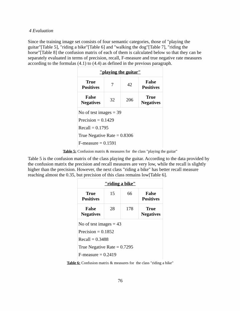
4 Evaluation

Since the training image set consists of four semantic categories, those of "playing the guitar"[Table 5], "riding a bike"[Table 6] and "walking the dog"[Table 7], "riding the horse"[Table 8] the confusion matrix of each of them is calculated below so that they can be separately evaluated in terms of precision, recall, F-measure and true negative rate measures according to the formulas (4.1) to (4.4) as defined in the previous paragraph.

"playing the guitar"

True Positives

7 42False

Positives

False Negatives

32 206True

Negatives

No of test images = 39

Precision = 0.1429

Recall = 0.1795

True Negative Rate = 0.8306

F-measure = 0.1591

Table 5: Confusion matrix & measures for the class "playing the guitar"

Table 5 is the confusion matrix of the class playing the guitar. According to the data provided by the confusion matrix the precision and recall measures are very low, while the recall is slightly higher than the precision. However, the next class "riding a bike" has better recall measure reaching almost the 0.35, but precision of this class remains low[Table 6].

"riding a bike"

True Positives

15 66 False Positives

False Negatives

28 178 True Negatives

No of test images = 43

Precision = 0.1852

Recall = 0.3488

True Negative Rate = 0.7295

F-measure = 0.2419

Table 6: Confusion matrix & measures for the class "riding a bike"

76

4 Evaluation

In comparison to the rest of classes, the class "walking the dog"[Table 7] has the worst performance, with very low precision and recall measures. This is something, though to be expected since the image part identifying unique the image is one more dogs that are relatively very small and in most of the cases not well segmented by the segmentation algorithm[Figure 37].

Figure 37: Segmentation Results for the class "walking the dog"; Left: good segmentation Right: not good segmentation

"walking the dog"

True Positives

6 43 False Positives

False Negatives

37 201 True Negatives

No of test images = 43

Precision = 0.1225

Recall = 0.1395

True Negative Rate = 0.8238

F-measure = 0.1305

Table 7: Confusion matrix & measures for the class "walking the dog"

The last class "riding a horse" is the one with the the highest precision and recall measures as shown in the table[Table 8] below. This can also be easily explained due to the unique shape of the horse[Figure 38] which in the cases where it is well segmented can not be confused with any of the elements of the other class.

77

4 Evaluation

"riding a horse"

True Positives

62 46 False Positives

False Negatives

100 79 True Negatives

No of test images = 162

Precision = 0.5741

Recall = 0.3827

True Negative Rate = 0.6320

F-measure = 0.4593

Table 8: Confusion matrix & measures for the class "riding a horse"

Figure 38: Segmentation Results for the class "riding a horse"; Left: good segmentation Right: not good segmentation

The whole Content-based Image Retrieval system performance has been compared to the lower limit, which in this case was chosen to be the randomness, since it would be pretty unfair to compare this unsupervised approach to any state to the art human action classification systems that use manually annotated images with the exact parts of the image revealing the particular characteristics of each action. The random system classified 10 times randomly each of the images of the test set and for each run the measures of precision and recall were computed. The proposed system performs slightly better with overall precision 0.2562 against the baseline, which achieved 0.2487. The recall measure of the proposed system also was higher being 0.2604 and the baseline lying around 0.2434. Therefore, we can conclude that the system performance, even if it is better than the chosen baseline it is still very poor, and further improvements should be carried out.

78

4 Evaluation

4.2.1.2.1 Error Analysis

All in all, the Content-based Image Retrieval does not perform well. The first reason is the not proper tuning of the segmentation parameters of the segmentation algorithm[Figure 39 & 40]. With the current implementation the same segmentation parameters are used for each image, while images used are natural with different illumination and viewpoint conditions. The universal segmentation algorithm does not exist therefore, such segmentation problems are to be expected.

Figure 39: Segmentation Results for the class "riding a bike" ; Left: good segmentation Right: not good segmentation

Consequently the selection of the number of the images out of which the ones that are retrieved is not the optimal one as already shown in the Table 4 and discussed in the previous paragraph. A further analysis should be carried out in the future work to improve the Content-based Image Retrieval System which definitely influences dramatically the final result.

Figure 40: Segmentation Results for the class "playing the guitar"; Left: good segmentation Right: not good

segmentation

79

4 Evaluation

4.2.2 Evaluation of Natural Language Processing System

The Natural Language Processing System was also separately evaluated. However, only the final output of the system was evaluated. In other words, the black box evaluation method was selected. The task was considered as a Machine Translation task and therefore the BLEU score metric as introduced in the Evaluation Overview. In other words, both information extraction and language generation were evaluated with the BLEU score. For each of the test images there is a reference description as given by the annotators. To guarantee that the description will be relevant to the reference sentence. The CBIR system is readjusted so that it feeds all the descriptions corresponding to the name of the test image. The sentence that the system produces in the end, is compared to the reference description.

The above procedure was run twice; once with input data the original descriptions produced by the annotators, including those where the annotation guidelines were not respected by the annotators and the average BLEUoriginal was estimated to 0.225. In Table 9 and Figure 41, the distribution of BLEU scores is available.

BLEU Score Bins Average BLEU Score per bin

Distribution

[0.0 - 0.1) 0.0032 35.89%

[0.1 - 0.2) 0.1595 8.36%

[0.2 - 0.3) 0.2424 21.60%

[0.3 - 0.4) 0.3340 8.36%

[0.4 - 0.5) 0.4531 19.86%

[0.5 - 0.6) 0.5362 1.74%

[0.6 - 0.7) 0.6903 0.70%

[0.7 - 0.8) 0.7559 3.48%

[0.8 - 0.9) - 0.00%

[0.9 - 1.0) - 0.00%Table 9: BLEU score Distribution for the modified descriptions as training and testing set

80

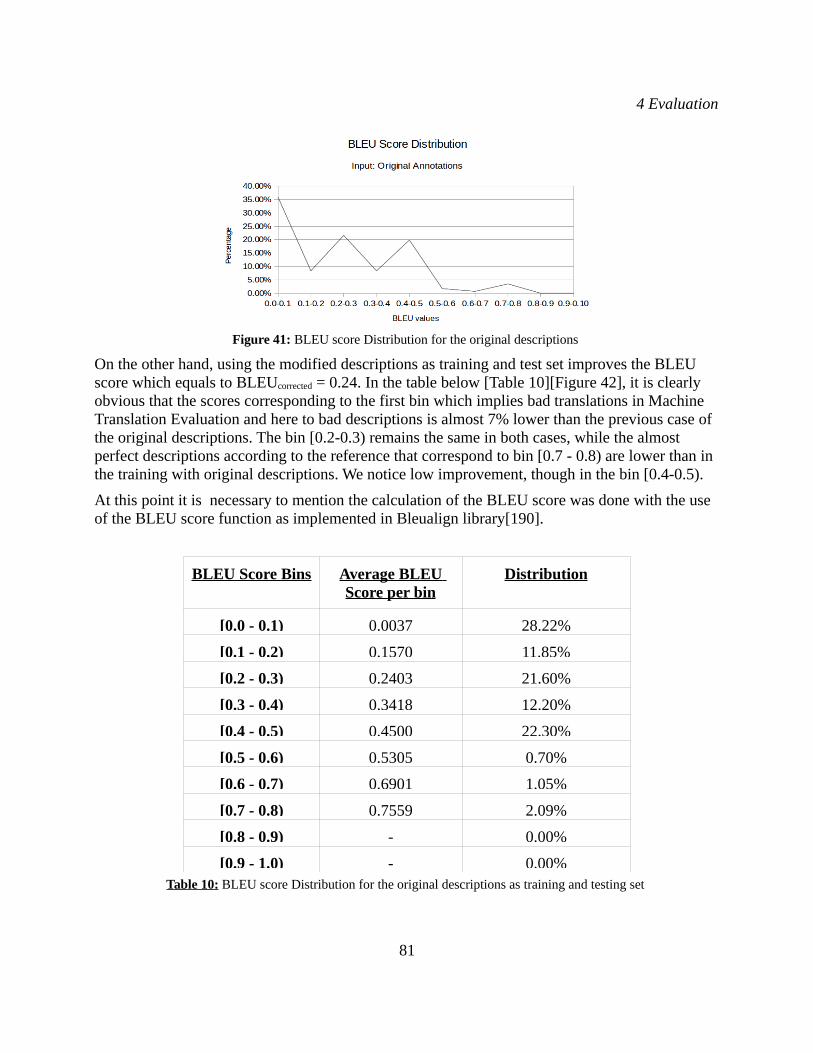
4 Evaluation

Figure 41: BLEU score Distribution for the original descriptions

On the other hand, using the modified descriptions as training and test set improves the BLEU score which equals to BLEUcorrected = 0.24. In the table below [Table 10][Figure 42], it is clearly obvious that the scores corresponding to the first bin which implies bad translations in Machine Translation Evaluation and here to bad descriptions is almost 7% lower than the previous case of the original descriptions. The bin [0.2-0.3) remains the same in both cases, while the almost perfect descriptions according to the reference that correspond to bin [0.7 - 0.8) are lower than in the training with original descriptions. We notice low improvement, though in the bin [0.4-0.5).

At this point it is necessary to mention the calculation of the BLEU score was done with the use of the BLEU score function as implemented in Bleualign library[190].

BLEU Score Bins Average BLEU Score per bin

Distribution

[0.0 - 0.1) 0.0037 28.22%

[0.1 - 0.2) 0.1570 11.85%

[0.2 - 0.3) 0.2403 21.60%

[0.3 - 0.4) 0.3418 12.20%

[0.4 - 0.5) 0.4500 22.30%

[0.5 - 0.6) 0.5305 0.70%

[0.6 - 0.7) 0.6901 1.05%

[0.7 - 0.8) 0.7559 2.09%

[0.8 - 0.9) - 0.00%

[0.9 - 1.0) - 0.00%Table 10: BLEU score Distribution for the original descriptions as training and testing set

81

4 Evaluation

Figure 42: BLEU score Distribution for the modified descriptions

4.2.2.1 Error Analysis

Some of the problems identified in this step, even if they are not statistically that high are some grammatical mistakes like the use of article in front of personal pronouns. Moreover, sometimes they text output produced by the system are incomplete, lacking a subject. In addition to that, even if the action is identified correctly and the verbs that represent the action and their complements are well identified, the subjects do not correspond to the reference descriptions.

As for the evaluation method, at this point we should mention that the shorter the reference descriptions they are, the more the possibility we get a higher BLEU score. For instance the cases that fall in the bin [0.0-0.1) even if semantically they have the same meaning, the reference descriptions may include a lot of redundant information that the system is not designed to capture. However, the system manages to extract the common knowledge no matter how long or short the training descriptions. This is something that is not favoured by the BLEU score and definitely a better evaluation method should be used in the future work.

To conclude, the BLEU score is not that far from what is supposed to be understandable text. The language part is also evaluated in the qualitative evaluation for the assessment of the whole system performance.

In Appendix II, there are examples of the system output versus the reference descriptions for several BLEU scores, for the training of the system with both of the datasets, the one with the original descriptions and the other with the modified descriptions.

82

4 Evaluation

4.2.3 Overall System Qualitative Evaluation

After the modular evaluation of the system, where the two main subsystems were evaluated separately, a qualitative research was carried out with the use of a questionnaire. There were 3 participants in total, that had to fill in a questionnaire of 12 questions for each of the output descriptions and their corresponding images.

The first assessor, being a non-native speaker, but having a proficiency in English language evaluated the whole number of test images, while the other two evaluated the 30 images that correspond to the images used to check the intra-annotator agreement of the first assessor. The other two assessors are not native speakers either, one of them with proficient level and the other with basic knowledge of English. The choice of the last one, was made motivated by the fact that the training set is the product of non native speakers and in many case from speakers not with very good knowledge of the language.

In all cases, there was a short tutorial, in order to make sure that the subjects understood the questions. All assessors were checked for intra-annotator agreement in two ways. The first way was with each questionnaire itself, since there were 3 questions measuring the same variable and they were used to verify how consistent the evaluators were with their answers. On the other hand, for all of them 10% of their images were shown twice.

Moreover, the inter-annotator agreement was calculated according to Cohen' Kappa coefficient[189] was calculated for the 30 common images that all of the annotators evaluated.

4.2.3.1 Inter-annotator agreement

Cohen's Kappa[189] measures the reliability of manual annotations. It takes into account the agreement occurring by chance.

κ=Pa−Pe

1−Pe

(4.5), where

Pa are the relative observed agreement between annotators,

Pe is the probability of agreement by chance.

The interpretation of the Kappa coefficient according to AMTA 2010 is the following:

• 0.0 - 0.2: slight agreement

• 0.2 - 0.4: fair agreement

• 0.4 - 0.6: moderate agreement

• 0.6 - 0.8: substantial agreement

• 0.8 - 1.0: near perfect agreement

83

4 Evaluation

As the results shown in Table 11 the Intra-annotator agreement is high for all the annotators, calculated with the formula 4.5. On the other hand, the overall inter-annotator a agreement for the three annotators is not very high with the Kappa coefficient being equal 0.56. The inter-annotator agreement concerning the language part is 0.59. The Inter-annotator agreement of the proficient in English annotators for the whole questions is 0.74 and therefore significantly better than the inter-annotator agreement of all the assessors. The inter-annotator agreement of the two proficient in English annotators concerning the language part is also significantly higher and equals 0.69. To conclude the inter-annotator agreement of the two proficient in English assessors improves from moderate agreement to substantial agreement.

Annotator P(A) P(E) Kappa

Annotator 1 0.90 0.25 0.87

Annotator 2 0.86 0.25 0.81

Annotator 3 0.92 0.25 0.89Table 11: Intra-annotator Agreement

4.2.3.2 Questionnaire Objectives

The objectives of the questionnaire are the following:

• Check if the human action was captured by the system.

• Check if the main objects and subjects are identified by the system.

• General evaluation of the adequacy of the image description produced by the system.

• Check the clarity of the meaning of the sentence.

• Check the quality of fluency in language according to the definitions of fluency as introduced in the Evaluation Overview.

• Check if there are grammatical errors and if they influence the understanding of the sentence content.

• Check if there are lexical errors and if they influence the understanding of the sentence content.

• Check if the sentence produced by the system is complete.

84

4 Evaluation

4.2.3.3 Cognitive metric scales

The cognitive metric scales used were based on those as suggested by EuroMatrix[185] for qualitative evaluation of Machine Translation. Moreover, the Likert scale is used while also for two questions the binary scale "Yes/No" was used in order to evaluate if the grammatical and lexical errors according to their frequency whether the influence the total understand of the sentence or not.

The following metrics were exactly used like that to measure the fluency, the adequacy and the clarity:

The EuroMatrix evaluators[185] used the following five point scale to measure fluency:

5 Flawless English

4 Good English

3 Non native English

2 Dis-fluent English

1 Incomprehensible

The scale used for evaluating adequacy was developed for the annual NIST Machine Translation Evaluation Workshop by the Linguistics Data Consortium . and is:

5 All

4 Most

3 Much

2 Little

1 None

The metric scale used for the clarity of the meaning of the sentence is:

3 Meaning of sentence is perfectly clear on first reading

2 Meaning of sentence is clear only after some reflection

1 Some, although not all, meaning is able to be gleaned from the sentence with some effort

0 Meaning of sentence is not apparent, even after some reflection

4.2.3.4 Questionnaire Results - Analysis

The following paragraphs shortly discuss the evaluation results for each of the annotators for each of the variables being examined by the questionnaire, the overall description evaluation, the human activity recognition, the subject & object recognition, language fluency, grammatical errors, lexical errors , sentence completeness and sentence clarity. Moreover, for each of the

85

4 Evaluation

variables mentioned before, a statistic table showing the distribution of the answers per annotator are presented. For Annotator 1, there are two tuples, one for the whole test set and the other for the descriptions corresponding to the descriptions assessed by Annotator 2 and Annotator 3. For each of the variables there is a graph were the discrete values where interpolate by a curve in order to make the visualisation easier and the comparison of the trends. More graphs, concerning the evaluation of each of the assessors is available in Appendix IV.

Last but not least, the sentences generated by the system in this part of the evaluation where chosen based on the highest BLEU score and therefore the training and test sets used here are those with the modified descriptions and not the original ones.

4.2.3.4.1 Overall Description Evaluation

In order to judge the overall rating of the system, the assessors answered a variation of a question 3 times as mentioned before in order to check the intra-annotator consistency. In Table 12 is the intra-annotator accuracy of each assessor for the questions 3, 4, and 6 of the questionnaire(for more information see Appendix III).

Annotator Kappa

Annotator 1 0.88

Annotator 2 0.91

Annotator 3 0.96Table 12: Kappa Q3, Q4, Q6

As far as the results of the evaluation of the overall description as produced by the systems and the conclusions we can reach from them, are concerned as we can see from the interpolated curves of the Figure 43, the distributions of all the users seem to follow the same pattern. The numbers in the table below [Table 13] show that the percentages per annotators do not correspond but the curves show that the assessors agree on the fact that the descriptions generated by the system do not describe well the corresponding to them image. The sum of the percentages of answers 1 & 2 for all of the annotators are about 65% to 70%. This is something to be expected also from the previous evaluation of the system, since it corresponds to the error rate percentage of the Content-based Image Retrieval System Evaluation. On the other hand, we also see that the sum of agreement scores and strongly agreement scores are diversified from about 18% up to 34%. Therefore we cannot reach any conclusions about agreement on the percentage of images described well by the system.

86

4 Evaluation

Annotators 1 2 3 4 5

Annotator 1all 34.35% 36.26% 0.76% 9.92% 18.70%

Annotator 1 25.93% 44.44% 3.7% 14.81% 11.11%

Annotator 2 17.86% 50.00% 14.29% 14.29% 3.57%

Annotator 3 44.83% 20.69% 0.00% 17.24% 17.24%Table 13: The distribution of the overall system evaluation per assessor, where 1- Strongly disagree, 2 - Disagree, 3

- Neither agree nor disagree, 4 - Agree , 5 - Strongly agree

Figure 43: The distribution of the overall system evaluation per assessor, where 1- Strongly disagree, 2 - Disagree, 3 - Neither agree nor disagree, 4 - Agree , 5 - Strongly agree

4.2.3.4.2 Human Activity Recognition

Concerning the correct human activity recognition as expected from the evaluation of the Content-based Image Retrieval system it lies between 27% and 33%. There is however not total agreement between all the users on whether the system does not identify correctly the human action. Annotator 2 expresses an uncertainty of 10%[Table 14].

Annotators 1 2 3 4 5

Annotator 1all 70.03% 0.70% 1.74% 0.35% 27.18%

Annotator 1 70.00% 0.00% 0.00% 0.00% 30.00%

Annotator 2 36.67% 20.00% 10.00% 0.00% 33.33%

Annotator 3 53.33% 13.33% 0.00% 3.33% 30.00%Table 14: The distribution of the human activity recognition per assessor, where 1- Strongly disagree, 2 - Disagree,

3 - Neither agree nor disagree, 4 - Agree , 5 - Strongly agree

87

4 Evaluation

The curves of Figure 44 do not follow the same pattern and therefore the only conclusion we can reach is just on the cases of agreement to the right human activity recognition which corresponds to the CBIR accuracy measure.

Figure 44: The distribution of the human activity recognition per assessor, where 1- Strongly disagree, 2 - Disagree, 3 - Neither agree nor disagree, 4 - Agree , 5 - Strongly agree

4.2.3.4.3 Subject & Object Recognition

The correct subject and object recognition was measured, just to verify the fact that the subjects captured correctly was random since the system was not adequately trained on that. As we can see, however there is not any sign of inter-annotator agreement both of the numbers of the Table 15 and the curves of the Figure 45.

Annotators 1 2 3 4 5

Annotator 1all 34.15% 3.48% 16.72% 29.62% 16.03%

Annotator 1 23.33% 3.33% 30.00% 33.33% 10.00%

Annotator 2 23.33% 30.00% 26.67% 6.67% 13.33%

Annotator 3 16.57% 6.67% 46.67% 13.33% 16.67%Table 15: The distribution of subject and object recognition per assessor, where 1- Strongly disagree, 2 - Disagree, 3

- Neither agree nor disagree, 4 - Agree , 5 - Strongly agree

88

4 Evaluation

Figure 45: The distribution of subject and object recognition per assessor, where 1- Strongly disagree, 2 - Disagree, 3 - Neither agree nor disagree, 4 - Agree , 5 - Strongly agree

4.2.3.4.4 Overall Language Evaluation - Language Fluency

From this section and on, the variables that are evaluated are related to the quality of the language. The current section discusses the result of language fluency. It is worth it mentioning that the question and the scale used to measure this variable are from EuroMatrix[185]. The scale is from 1 to 5, with 1 corresponding to incomprehensible language while 5 meaning flawless language. What is worth mentioning here is that there is an agreement around 80%[Table 16 & Figure 46] on flawless language which is better that the BLEU score, something to be expected though since as we mentioned before the BLEU score has not been the best measure to evaluate the quality of language output of the system.

Annotators 1 2 3 4 5

Annotator 1all 3.83% 2.79% 8.36% 3.14% 81.88%

Annotator 1 0.00% 0.00% 10.00% 3.33% 86.67%

Annotator 2 0.00% 10.00% 3.33% 6.67% 80.00%

Annotator 3 0.00% 0.00% 10.00% 10.00% 80.00%Table 16: The distribution of the language fluency per assessor, where 1- Incomprehensible , 2 - Dis-fluent English,

3 - Non native English, 4 - Good English, 5 - Flawless English

89

4 Evaluation

Figure 46: The distribution of the language fluency per assessor, where 1- Incomprehensible , 2 - Dis-fluent English, 3 - Non native English, 4 - Good English, 5 - Flawless English

4.2.3.4.5 Grammatical Errors

The assessors had also to evaluate the amount of grammatical errors per sentence and their influence in the whole sentence understanding. What is really encouraging is that the system has very low percentages from several to too many mistakes, while also high agreement on zero mistakes[Table 17 & Figure 47]. There are, however, around 15% of the sentences identified by the majority with a few mistakes.

Annotators 1 2 3 4 5

Annotator 1all 86.76% 7.32% 3.14% 0.35% 2.44%

Annotator 1 93.33% 6.67% 0.00% 0.00% 0.00%

Annotator 2 86.67% 10.00% 3.33% 0.00% 0.00%

Annotator 3 83.33% 13.33% 3.33% 0.00% 0.00%Table 17: The distribution of grammatical error evaluation per assessor, where 1 - Zero , 2 - Few , 3 - Several , 4 -

Many , 5 - Too many

In this part of the evaluation, assessors were also asked whether the grammatical mistakes affected the whole text understanding. Annotator 2 and Annotator 3 that evaluated only 10% of the test set, both agreed that the grammatical mistakes had to influence in the understanding of the sentence, while Annotator 1 that evaluated the total amount of the training set agrees that in 4.18% of the grammatical errors did not allow to understand the sentence generated by the system.

In any case the percentage is very low and as we can see from the interpolated curves in Figure 47 there is high agreement on the fact that the system generates sentences with either non or a few mistakes.

90

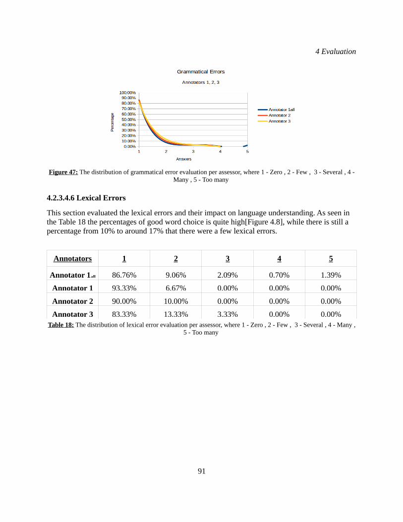
4 Evaluation

Figure 47: The distribution of grammatical error evaluation per assessor, where 1 - Zero , 2 - Few , 3 - Several , 4 - Many , 5 - Too many

4.2.3.4.6 Lexical Errors

This section evaluated the lexical errors and their impact on language understanding. As seen in the Table 18 the percentages of good word choice is quite high[Figure 4.8], while there is still a percentage from 10% to around 17% that there were a few lexical errors.

Annotators 1 2 3 4 5

Annotator 1all 86.76% 9.06% 2.09% 0.70% 1.39%

Annotator 1 93.33% 6.67% 0.00% 0.00% 0.00%

Annotator 2 90.00% 10.00% 0.00% 0.00% 0.00%

Annotator 3 83.33% 13.33% 3.33% 0.00% 0.00%Table 18: The distribution of lexical error evaluation per assessor, where 1 - Zero , 2 - Few , 3 - Several , 4 - Many ,

5 - Too many

91

4 Evaluation

Figure 48:The distribution of lexical error evaluation per assessor, where 1 - Zero , 2 - Few , 3 - Several , 4 - Many , 5 - Too many

In this case, also Annotator 2 and Annotator 3 did not mention having any influence in the sentence understanding due to the use of wrong words, while the Annotator 1 that evaluated all the images and the corresponding descriptions of the test set identifies a 6.62% of the cases where the use of not the appropriate words influenced the understanding of the sentence.

4.2.3.4.7 Sentence Completeness

In terms of sentence completeness, there is also high agreement[Figure 49] on the fact that the sentences generated by the system were complete. There is, however a percentage between 3% and 13%, where the sentences were marked as incomplete. The whole distribution is shown in Table 19.

Annotators 1 2 3 4 5

Annotator 1all 84.32% 1.74% 1.05% 7.67% 5.23%

Annotator 1 93.33% 0.00% 0.00% 6.67% 0.00%

Annotator 2 83.33% 3.33% 10.00% 0.00% 3.33%

Annotator 3 90.00% 6.67% 0.00% 0.00% 3.33%Table 19: The distribution of sentence completeness per assessor, where 1- Strongly disagree, 2 - Disagree, 3 -

Neither agree nor disagree, 4 - Agree , 5 - Strongly agree

92

4 Evaluation

Figure 49: The distribution of sentence completeness per assessor, where 1- Strongly disagree, 2 - Disagree, 3 - Neither agree nor disagree, 4 - Agree , 5 - Strongly agree

4.2.3.4.8 Sentence Clarity - Meaning adequacy

The last variable evaluated by means of the questionnaire is the sentence clarity. In this case the adequacy of the meaning of the sentence ignoring the correspondence to the actual content of the meaning was also rated very high by all the assessors, lying approximately on 86%. The curves in Figure 50 also seem to follow the same pattern and therefore there were very few cases that the sentence meaning would not be understood at all. As expected from the evaluation of the influence of grammatical and lexical errors in language understanding, we see that Annotators 2 and 3 did not identify any cases were the meaning of the sentence was not grasped at all[Table 20].

Annotators 0 1 2 3

Annotator 1all 3.48% 4.18% 4.53% 87.80%

Annotator 1 0.00% 3.33% 3.33% 93.33%

Annotator 2 0.00% 3.33% 10.00% 86.67%

Annotator 3 0.00% 0.00% 13.33% 86.67%Table 20: The distribution of sentence clarity per assessor, where 0 - Meaning of sentence is not apparent, even after some reflection , 1 - Some, although not all, meaning is able to be gleaned from the sentence with some effort , 2 - Meaning of sentence is clear only after some reflection , 3 - Meaning of sentence is perfectly clear on first reading

93

4 Evaluation

Figure 50: The distribution of sentence clarity per assessor, where 0 - Meaning of sentence is not apparent, even after some reflection , 1 - Some, although not all, meaning is able to be gleaned from the sentence with some effort ,

2 - Meaning of sentence is clear only after some reflection , 3 - Meaning of sentence is perfectly clear on first reading

4.3 Discussion on the Results

As show from the results of the previous paragraphs the system proposed in this master thesis has its strengths and weaknesses. The task of automatic image summarisation is quite complicated composed by two main components that join two different research fields of Artificial Intelligence, those of Computer Vision and Natural Language Processing. Each module of them consists of sub-modules that affect a lot the performance of the overall system. The Computer Vision module which corresponds to a Content-based Image Retrieval System as shown by the results above, does not perform very satisfactorily and fails to outperform other Content-based Image Retrieval systems. However, we should not immediately reject this approach, since there is evidence that the performance of the system could be improved with the use of a segmentation algorithm that can segment properly the images. The performance of the current algorithm varies from very good segmented images to very bad, which of course happens due to the variation of images and due to the fact a big amount of the images is very noisy and the not always good tuning of the segmentation parameters. Moreover, the CBIR system works pretty well in the case of images with horses, something that can be justified by the unique shape of horses, which was in most of the cases properly segmented.

On the other hand, the Natural Language Processing System performs a lot better, even if the BLEU score evaluation turned out to be very strict. The qualitative evaluation in terms of the language part rated the language fluency and clarity very high, even if in most of the cases the language content did not correspond to the image content. The consistence of the BLEU score is a good indicator that the not proper input to the system which is considered noise and was expected to produce poor descriptions, was a hypothesis that prove to be wrong. So the system is quite robust to the noise even if its performance improves slightly with the modified descriptions and the noise elimination. This can be explained due to the fact that Stanford dependencies are named and they capture cases of incomplete sentences as system input or sentences with lack verb which in our case is very important to capture the main human action. The main effect of the

94

4 Evaluation

noisy input occurs in the cases where just images with incomplete or non human action relevant descriptions are retrieved.

Last but not least, as already mentioned before the qualitative evaluation by means of the questionnaire offers better results in terms of language fluency, adequacy, lack of significant lexical and grammatical errors while also the sentence completeness with a significant lying on 0.69 inter-annotator agreement. Finally, the evaluation of the CBIR are also verified by the questionnaire results.

Future work on the points mentioned before, which relate to the Content-based Image Retrieval can guarantee and improved version of the system with better results. Some more rules on the optimal path extraction could eventually capture more information, but this is something to be done only when the respective adjustments are made to guarantee that this information correspond to the visual image content.

95

96

5 Summary & Conclusions

5 Summary & Conclusions

This work has addressed the issue of Image Summarisation, and more specifically the automatic description of human actions from static images. The issue has been dealt as a combination of two different research fields of Artificial Intelligence, those of Computer Vision and Natural Language Processing. The work has been organised in three parts.

Firstly, a short overview of the related work was presented by grouping it into three categories, by approaches that produce a set of words from images, the approaches that produce text where the relations between the words are maintained and finally some methods of generating language given video or image sequences as input. The method proposed in this dissertation, differs in the sense that tries to combine the unsupervised Image Processing part of the first group of approaches with the structured Natural Language Processing parts of the second group of approaches, having as a goal to output descriptions where the semantic relations between the words are guaranteed. Therefore, the proposed system consists of two sub-systems, those of Content-based Image Retrieval and Natural Language Processing, with the second sub-system consisting of an Information Extraction System and a rule-based Natural Language Generation Surface Processing system.

Before the system implementation, time was invested in creating the appropriate dataset for this specific task. A dataset of images consisting of four semantic categories showing human actions and activities was annotated my volunteers. For this purpose an annotation platform was created based on the idea of crowd sourcing in order to collect human annotations for the training and testing datasets. The evaluation of the Natural Language Processing sub-system was made with two datasets one on the original annotations as provided by the users and another set consisting of the corrections of the errors made by the users, in order to check how sensitive the system is to noisy input. Therefore when the annotations were gathered a correction procedure of mistakes caused due to bad use of English, lack of main verb, lack of auxiliary verb, lack of verb showing human activity or action, use of anaphoric expressions without the use of antecedent, or even spelling and typographical mistakes.

The proposed system has been composed by two parts, a Content-based Image Retrieval part and a Natural Language Processing part. Given a query image the first part retrieves a set of images perceived as visually similar and the second part processes the annotations following each of the images in order to extract common information by using a graph merging technique of the dependency graphs of the annotated sentences. An optimal path consisting of a subject-verb-complement relation is extracted and transformed into a proper sentence by applying a set of surface processing rules.

The evaluation of the system was carried out in three different ways. Firstly, the Content-based Image Retrieval sub-system was evaluated in terms of precision and recall and compared to a baseline classification system based on randomness. The system accuracy of the image retrieval is better than the baseline but still very low, which as occurred from the error analysis is due to the bad tuning of the segmentation parameters and the noisy nature of the images. In future work,

97

5 Summary & Conclusions

a better implementation of the Content-based Image Retrieval part is required in order to improve the overall system performance, since the Content-based Image Retrieval system, as first in the implementation pipeline influences the content of the information extraction and therefore the final description.

In order to evaluate the Natural Language Processing sub-system, the Image Summarisation task was considered as a machine translation task, and thus it was evaluated in terms of BLEU score. Given images that correspond to the same semantic as a query image the system output was compared to the corresponding reference summary as provided during the annotation phase, in terms of BLEU score. The BLEU score even if it proves to be a strict evaluation metric, it can be interpreted for the average of images as understandable, with the smallest reference description guaranteeing a very high BLEU score. Moreover, the BLEU score was slightly higher in the case of the corrected annotation, meaning that the Natural Language Processing is robust to noise.

Finally, the whole system has been qualitatively evaluated by means of a questionnaire, that evaluated the overall system output not very satisfactory. However, the performance of the Natural Language Processing system was rated very well with very high inter-annotator agreement, in terms of fluency, meaning adequacy and completeness, while only very few grammatical and lexical errors were identified, that did not influence though, the understanding of the sentence meaning.

To conclude, the evaluation of the Natural Language Processing system is very good and in future work an improvement in the Content-based Image Retrieval is necessary in order to improve the overall system performance.

98

References

References [1] Denis Simakov, (2008). Visual summarisation of Images and Video. Thesis submitted in partial fulfillment of the requirements for the degree of Ph.D., Under the Supervision of Michal Irani, Faculty of Mathematics and Computer Science, The Weizmann Institute of Science.

[2] Pinaki Sinha, (2011). Automatic Summarisation Of Personal Photo Collections. Dissertation Submitted In Partial Satisfaction Of The Requirements For The Degree Of Doctor Of Philosophy In Information And Computer Science, University Of California, Irvine.

[3] Esteban L. & Hoang D., (1996). The connection array for image summarisation. Source: Mathematics and Computers in Simulation, Volume 41, Number 1, June 1996 , pp. 75-86(12), Publisher: Elsevier.

[4] Ali Farhadi, Mohsen Hejrati, Mohammad Amin Sadeghi, Peter Young, Cyrus Rashtchian, Julia Hockenmaier, David Forsyth, (2010). Every Picture Tells a Story: Generating Sentences from Images. Computer Vision ECCV 2010, Lecture Notes in Computer Science Volume 6314, 2010, pp 15-29.

[5] Gerd Herzog, Karl Rohr, (1995). Integrating Vision and Language: Towards Automatic Description of Human Movements. KI-95: Advances in Artificial Intelligence. 19th Annual German Conference on Artificial Intelligence.

[6] Margaret Mitchell, Xufeng Han, Jeff Hayes, (2012). Midge: Generating Descriptions of Images., INLG 2012 Proceedings of the 7th International Natural Language Generation Conference, pages 131-133.

[7] Amir Sadovnik, Yi-I Chiu, Noah Snavely , Shimon Edelman, Tsuhan Chen, (2012). Image Description with a Goal: Building Efficient Discriminating Expressions for Images. In CVPR(2012)2791-2798.

[8] Patrick Hède, Pierre-Alain Mollic, Jol Bourgeoys, Magali Joint, Corinne e Thomas, (2004). Automatic generation of natural language descriptions for images. RIAO 2004 Avignon France 26-28 April

[9] Girish Kulkarni, Visruth Premraj, Sagnik Dhar, Siming Li, Yejin Choi, Alexander C Berg, Tamara L Berg, (2011). "Baby Talk: Understanding and Generating Image Descriptions", Proceedings of the 24th CVPR.

[10] Yansong Feng and Mirella Lapata, (2010). How Many Words is a Picture Worth? Automatic Caption Generation for News Images, Proceedings of the 48th Annual Meeting of the Association for Computational Linguistics, pages 12391249, Uppsala, Sweden, 11-16 July 2010.

[11] Benjamin Z. Yao, Xiong Yang, Liang Lin, Mun Wai Lee and Song-Chun Zhu, (2010). I2T: Image Parsing to Text Description. Proceedings of the IEEE (Volume:98 , Issue: 8 ), August 2010.

[12] Dirk Voelz, Elisabeth André, Gerd Herzog and Thomas Rist, (1998). Rocco: A RoboCup Soccer Commentator System.

99

References

[13] E. André, G. Herzog, and T. Rist, (1994). Multimedia Presentation of Interpreted Visual Data. In P. Mc Kevitt, editor, Proc. of AAAI-94 Workshop on Integration of Natural Language and Vision Processing", pages 74-82, Seattle, WA.

[14] E. André, G. Herzog, and T. Rist, (1988). On the Simultaneous Interpretation of Real World Image Sequences and their Natural Language Description: The System SOCCER. In Proc. of the 8th ECAI, pages 449-454, Munich, Germany.

[15] Gupta, A., Srinivasan, P., Shi, J., Davis, L., (2009). Understanding videos, constructing plots: Learning a visually grounded storyline model from annotated videos. In: CVPR.

[16] Luo, J., Caputo, B., Ferrari, V., (2009). Whos doing what: Joint modeling of names and verbs for simultaneous face and pose annotation. In: NIPS.

[17] S. Li, G. Kulkarni, T. L. Berg, A. C. Berg, and Y. Choi, ( 2011). Composing simple image descriptions using web-scale n-grams. CoNLL 11.

[18] Pan, J., Yang, H., Duygulu, P., and Faloutsos, C. (2004). Automatic image captioning. In Proceedings of the 2004 International Conference on Multimedia and Expo, pages 19871990, Taipei.

[19] Mori, Y., Takahashi, H., and Oka, R. (1999). Image-to-word transformation based on dividing and vector quantizing images with words. In Proceedings of the 1st International Workshop on Multimedia Intelligent Storage and Retrieval Management, Orlando, FL.

[20] Moran, S. (2009). Automatic image tagging. Masters thesis, The University of Edinburgh.

[21] Mittal, V. O., Roth, S., Moore, J. D., Mattis, J., and Carenini, G. (1995). Generating explanatory captions for information graphics. In IJCAI95: Pro- ceedings of the 14th International Joint Conference on Artificial Intelligence, pages 12761283, San Francisco, CA, USA. Morgan Kaufmann Publishers Inc.

[22] Youakim Badr and Richard Chbeir, (2006 ). Automatic Image Description Based on Textual Data. Journal on Data Semantics VII, Lecture Notes in Computer Science Volume 4244, pp 196-218.

[23] Polina Kuznetsova, Vicente Ordonez, Alexander C. Berg, Tamara L. Berg and Yejin Choi, (2012). Collective Generation of Natural Image Descriptions. Proceeding ACL ’12 Proceedings of the 50th Annual Meeting of the Association for Computational Linguistics: Long Papers - Volume 1 Pages 359-368.

[24] V. Lavrenko, R. Manmatha, J. Jeon (2003). A Model for Learning the Semantics of Pictures. IN NIPS

[25] Yansong Feng (2011). Automatic Caption Generation for News Images. PhD Thesis, University of Edinburgh.

[26] Jiwoon Jeon and R. Manmatha, (2004). Using Maximum Entropy for Automatic Image Annotation. CIVR 2004: 24-32.

100

References

[27] Marta Sabou, Kalina Bontcheva, Arno Scharl, (2012). Crowdsourcing Research Opportunities: Lessons from Natural Language Processing. In: 12th International Conference on Knowledge Management and Knowledge Technologies, Special Track Research 2.0 (#STR20) , 5-7 September, Graz, Austria. (In Press)

[28] Vicente Ordonez, Girish Kulkarni, Tamara L Berg., (2011). Im2text: Describing images using 1 million captioned photographs. Proceedings of NIPS 2011.

[29] Chen, H.L. and Rasmussen, E.M. (1999). Intellectual access to images. Library Trends, Vol. 48 No. 2, pp. 291-302.

[30] Mehmet Sezgin and Bulent Sankur, (2004). Survey over image thresholding techniques and quantitative performance evaluation. Journal of Electronic Imaging 13(1), 146–165.

[31] Nobuyuki Otsu (1979). A threshold selection method from gray-level histograms. IEEE Trans. Sys., Man., Cyber.

[32] Gurjeet kaur Seerha et al. Review on Recent Image Segmentation Techniques. International Journal on Computer Science and Engineering (IJCSE).

[33] Rajeshwar Dass, Priyanka, Swapna Devi. Image Segmentation Techniques.

[34] Shankar Rao, Hossein Mobahi, Allen Yang, Shankar Sastry and Yi Ma (2009). Natural Image Segmentation with Adaptive Texture and Boundary Encoding. Proceedings of the Asian Conference on Computer Vision (ACCV), H. Zha, R.-i. Taniguchi, and S. Maybank (Eds.), Part I, LNCS 5994, pp. 135--146, Springer.

[35] Hossein Mobahi, Shankar Rao, Allen Yang, Shankar Sastry and Yi Ma (2011). Segmentation of Natural Images by Texture and Boundary Compression. International Journal of Computer Vision (IJCV), 95 (1), pg. 86-98, Oct. 2011.

[36] Sobel, I. (1990). An Isotropic 3×3 Gradient Operator, Machine Vision For Three – Dimensional Scenes. Freeman, H., Academic Pres, Ny, 376-379.

[37] Roberts, L. G. (1965). Machine Perception Of Three-Dimensional Solids. In Optical And Electro-Optical Information Processing ( J. Tippett, Ed.), 159-197, Mit Pres.

[38] Kirsch, R. (1971). Computer Determination Of The Constituent Structure Of Biological Images. Computers And Biomedical Research

[39] Marr, D.; Hildreth, E. (29 Feb 1980). Theory Of Edge Detection. Proceedings Of The Royal Society Of London. Series B, Biological Sciences 207 (1167): 187–217

[40] Canny, J. (1986). A Computational Approach To Edge Detection. IEEE Transactions On Pattern Analysis anad Machine Intelligence, 8, 679-700.

[41] Rolf Adams and Leanne Bischof (1994). Seeded Region Growing. IEEE Transactions on Pattern Analysis and Machine Intelligence, Vol. 16, No. 6, June 1994.

[42] X. Jiang, R. Zhang, S. Nie (2009). Image Segmentation Based on PDEs Model: a Survey. IEEE conference, pp. 1-4.

101

References

[43] Osher S, Sethian J A. (1988). Fronts propagating with curvature-dependent speed: algorithms based on Hamilton-Jacobi formulations[J]. Comput. Phys, 1988; 79(1), 12-49.

[44] Jianbo Shi and Jitendra Malik (2000). Normalized Cuts and Image Segmentation. IEEE Transactions on pattern analysis and machine intelligence, pp 888-905, Vol. 22, No. 8.

[45] Leo Grady (2006). Random Walks for Image Segmentation. IEEE Transactions on Pattern Analysis and Machine Intelligence, pp. 1768–1783, Vol. 28, No. 11.

[46] Z. Wu and R. Leahy (1993). An optimal graph theoretic approach to data clustering: Theory and its application to image segmentation. IEEE Transactions on Pattern Analysis and Machine Intelligence, pp. 1101–1113, Vol. 15, No. 11.

[47] Leo Grady and Eric L. Schwartz (2006). Isoperimetric Graph Partitioning for Image Segmentation. IEEE Transactions on Pattern Analysis and Machine Intelligence, pp. 469–475, Vol. 28, No. 3.

[48] C. T. Zahn (1971). Graph-theoretical methods for detecting and describing gestalt clusters. IEEE Transactions on Computers, pp. 68–86, Vol. 20, No. 1.

[49] Pedro F. Felzenszwalb and Daniel P. Huttenlocher (2004). Efficient Graph-Based Image Segmentation. International Journal of Computer Vision, Volume 59, Number 2, September 2004.

[50] Oxford Dictionaries. http://www.oxforddictionaries.com/

[51] WordNet, Princeton. http://wordnetweb.princeton.edu/perl/webwn

[52] H. Tamura, S. Mori, T. Yamawaki (1987). Textural Features Corresponding to Visual Perception. IEEE Trans. on Systems, Man and Cyber., June 1978, vol. 8, no. 6, p. 460–473.

[53] I. Fogel, D. Sagi (1989). Gabor filters as texture discriminator. Biological Cybernetics June 1989, Volume 61, Issue 2, pp 103-113.

[54] Robert M Haralick, K Shanmugam, Its'hak Dinstein (1973). Textural Features for Image Classification. IEEE Transactions on Systems, Man, and Cybernetics. SMC-3 (6): 610–621.

[55] A. Oliva and A. Torralba (2001). Modeling the shape of the scene: a holistic representation of the spatial envelope. IJCV, 42(3):145–175.

[56] David G. Lowe (2004). Distinctive image features from scale-invariant keypoints. International Journal of Computer Vision, 60, 2, pp. 91-110.

[57] H. Bay, A. Ess, T. Tuytelaars, L.V. Gool (2008). SURF: Speeded Up Robust Features. Computer Vision and Image Understanding (CVIU), June 2008, vol. 110, no. 3, p. 346–359.

[58] J. Sivic and A. Zisserman (2003). Video Google: A text retrieval approach to object matching in videos. In Proceedings of ICCV, volume 2, pages 1470–1477, Nice, France, Oct 2003.

[59] S. Beucher and F. Meyer (1992). The Morphological Approach to Segmentation: The Watershed Transformation. In book: Mathematical Morphology in Image Processing, Editors: Dougherty, E.R., pp.433–481. Chapter 12.

102

References

[60] Hunter, Richard Sewall (1948). Photoelectric Color-Difference Meter. In Proceedings of the Winter Meeting of the Optical Society of America, JOSA 38 (7): 661.

[61] Koen E. A. van de Sande, Theo Gevers, Cees G. M. Snoek (2010). Evaluating Color Descriptors for Object and Scene Recognition IEEE Transactions on Pattern Analysis and Machine Intelligence, Volume 32 (9), page 1582--1596.

[62] Michael J. Metternich, Marcel Worring and Arnold W.M. Smeulders (2010). Color Based Tracing in Real-Lfe Surveillance Data. In Transactions on Data Hiding and Multimedia Security V, LNCS 6010, pp 18-33.

[63] Yu, H., Li, M., Zhang, H.-J., Feng, J. (2002). Color texture moments for content-based image retrieval. In: Internat. Conf. on Image Processing, vol. 3, pp. 929–932.

[64] A. Bosch, A. Zisserman, and X. Muoz (2008). Scene classification using a hybrid generative/discriminative approach. IEEE Transactions on Pattern Analysis and Machine Intelligence, vol. 30, no. 04, pp. 712–727.

[65] J. van de Weijer, T. Gevers, and A. Bagdanov (2006). Boosting color saliency in image feature detection. IEEE Transactions on Pattern Analysis and Machine Intelligence, vol. 28, no. 1, pp. 150–156.

[66] A. Yamada, and E. Kasutani (2001). The MPEG-7 Color Layout Descriptor: A Compact Image Feature Description for High- speed Image/Video Segment Retrieval. ICIP, vol. 1, Oct. 2001, pp. 674–677.

[67] S.Selvarajah and S.R. Kodituwakku (2011). Analysis and Comparison of Texture Features for Content Based Image Retrieval. International Journal of Latest Trends in Computing (E-ISSN: 2045-5364) , Volume 2, Issue 1, March 2011.

[68] M. Sonka, V. Hlavac and R. Boyle (1999). Image processing, analysis and machine vision. PWS publishing, San Francisco.

[69] K. Laws (1980). Textured Image Segmentation. Ph.D. Dissertation, University of Southern California, January 1980.

[70] Mary M. (1975). Texture Analysis Using Gray Level Run Lengths , Computer Graphics And Image Processing 4, 172-179.

[71] Brenard J., (2005). Digital Image Processing, Springer-Verlag Berlin, Germany.

[72] Havlicek, J. P., Tay, P.C. (2001). Determination of the number of texture segments using wavelets. Electronic Journal of Differential Equations, Conf. pp 61–70.

[73] Hammouda, Khaled, and Ed Jernigan (2000). Texture segmentation using Gabor filters. Canada: Center for Intelligent Machines, McGill University.

[74] Mingqiang Yang, Kidiyo Kpalma, Joseph Ronsin (2012). Shape-Based Invariant Feature Extraction for Object Recognition. In Advances in Reasoning-Based Image Processing Intelligent : Systems Conventional and Intelligent Paradigms, Intelligent Systems Reference Library,

103

References

Volume 29, Roumen Kountchev and Kazumi Nakamatsu (Eds.) , Springer-Verlag Berlin Heidelberg , 2012, ISBN 978-3-642-24692-0

[75] Kauppinen, H.; Seppanen, T. & Pietikainen, M. (1995). An Experimental Comparison of Auto-regressive and Fourier-Based Descriptors in 2-D Shape Classification. IEEE Trans. Pattern Analysis and Machine Intelligence 17(2), 201-207.

[76] Zhang, D. & Lu, G. (2002). A Comparative Study of Fourier Descriptors for Shape Representation and Retrieval. In 'Proc. 5th Asian Conference on Computer Vision'.

[77] Yadava, R. B.; Nishchala, N. K.; Gupta, A. K. & K.Rastogi, V. (2007). Retrieval and classification of shape-based objects using Fourier, generic Fourier, and wavelet- Fourier descriptors technique: A comparative study. Optics and Lasers in Engineering 45(6), 695-708.

[78] Ming-Kuei Hu (1962 ). Visual Pattern Recognition by Moment Invariants, IEEE Transactions on Information Theory.

[79] F. Gregory Ashby and Daniel M. Ennis (2007). Similarity measures. Scholarpedia, 2(12):4116.

[80] Suzuki, Yu., Mitsukawa, M., Kawagoe, K. (2008). A Image Retrieval Method Using TFIDF Based Weighting Scheme. Published In: Database and Expert Systems Application, 2008. DEXA '08. 19th International Workshop, p.112 - 116.

[81] MacQueen, J. B. (1967). Some Methods for classification and Analysis of Multivariate Observations. Proceedings of 5th Berkeley Symposium on Mathematical Statistics and Probability 1. University of California Press. pp. 281–297. MR 0214227. Zbl 0214.46201. Retrieved 2009-04-07.

[82] Steinhaus, H. (1957). Sur la division des corps matériels en parties. Bull. Acad. Polon. Sci. (in French) 4 (12): 801–804. MR 0090073. Zbl 0079.16403.

[83] Arya, S., and D. M. Mount (1993). Algorithms for fast vector quantization. In: Proceedings of the Data Compression Conference 1993. : IEEE Press.

[84] Cunningham, P., and S. J. Delaney (2007). K-Nearest Neighbor Classifiers. Technical Report UCD-CSI-2007-4, School of Computer Science and Informatics, University College Dublin, Ireland.

[85] Friedman, J. H., J. L. Bentley, and R. A. Finkel (1977). 'An algorithm for finding best matches in logarithm expected time'. ACM Transactions on Mathematical Software, 3, 209-226.

[86] Mark Johnson (2012). Natural Language Processing and Computational Linguistics: from Theory to Application. Lecture slides.

[87] Robert Dale, Hermann Moisl & Harold Somers (eds) (2003). A Handbook of Natural Language Processing. New York: Marcel Dekker. ISBN 0824790006.

[88] Jurafsky, Daniel & James H. Martin (2000). Speech and Language Processing. New Jersey, USA: Prentice Hall.

104

References

[89] Ruslan Mitkov (1999). Anaphora Resolution: The State Of The Art.

[90] Jonathan H. Clark and José P. González-Brenes (2008). Coreference Resolution: Current Trends and Future Directions.

[91] Jurafsky, Dan (2004). Pragmatics and computational linguistics. In Laurence R. Horn and Gregory Ward, eds, Handbook of Pragmatics, 578-604 Oxford: Blackwell.

[92] Bunt Harry and Bill Black (2000). The ABC of computational pragmatics. Computational pragmatics: Abduction, belief and context, ed. by Harry C. Bunt and William Black. Amsterdam: John Benjamins.

[93] Joakim Nivre (2013). Syntactic Parsing. Lecture notes. Retrieved from: http://stp.lingfil.uu.se/~nivre/master/parsing.html

[94] T. L. Booth & R. A. Thompson (1973). Applying Probability Measures to Abstract Languages. IEEE Transactions on Computers C-22:442–450.

[95] H. Ney (1991). Dynamic Programming Parsing for Context-Free Grammars in Continuous Speech Recognition. IEEE Transactions on Signal Processing 39:336–340.

[96] A. Stolcke (1995). An Efficient Probabilistic Context-Free Parsing Algorithm that Computes Prefix Probabilities. Computational Linguistics 21:165–202.

[97] J. Eisner & G. Satta (1999). Efficent Parsing for Bilexical Context-Free Grammars and Head Automaton Grammars. In Proceedings of the 37th Annual Meeting of the Association for Computational Linguistics (ACL), pp. 457–464.

[98] E. Charniak (1996). Tree-Bank Grammars. In Proceedings of AAAI/IAAI, pp. 1031–1036.

[99] M. Johnson (1998). PCFG Models of Linguistic Tree Representations. Computational Linguistics 24:613–632.

[100] M. Collins (1997). Three Generative, Lexicalised Models for Statistical Parsing. In Proceedings of the 35th Annual Meeting of the Association for Computational Linguistics (ACL) and the 8th Conference of the European Chapter of the Association for Computational Linguistics (EACL), pp. 16–23.

[101] M. Collins (1999). Head-Driven Statistical Models for Natural Language Parsing. Ph.D. thesis, University of Pennsylvania.

[102] E. Charniak (2000). A Maximum-Entropy-Inspired Parser. In Proceedings of the First Meeting of the North American Chapter of the Association for Computational Linguistics (NAACL), pp. 132–139.

[103] S. Petrov, et al. (2006). Learning Accurate, Compact, and Interpretable Tree Annotation. In Proceedings of the 21st International Conference on Computational Linguistics and the 44th Annual Meeting of the Association for Computational Linguistics, pp. 433–440.

[104] E. Briscoe & J. Carroll (1993). Generalised probabilistic LR parsing of natural language (corpora) with unification-based grammars. Computational Linguistics 19:25–59.

105

References

[105] J. Carroll & E. Briscoe (1996). Apportioning Development Effort in a Probabilistic LR Parsing System through Evaluation. In Proceedings of the Conference on Empirical Methods in Natural Language Processing (EMNLP), pp. 92–100.

[106] F. Jelinek, et al. (1994). Decision Tree Parsing Using a Hidden Derivation Model. In Proceedings of the ARPA Human Language Technology Workshop, pp. 272–277.

[107] S. Clark & J. R. Curran (2004). Parsing the WSJ Using CCG and Log-Linear Models. In Proceedings of the 42nd Annual Meeting of the Association for Computational Linguistics (ACL), pp. 104–111.

[108] E. Charniak & M. Johnson (2005). Coarse-to-Fine n-Best Parsing and MaxEnt Discriminative Reranking. In Proceedings of the 43rd Annual Meeting of the Association for Computational Linguistics (ACL), pp. 173–180.

[109] Lucien Tesnière (1959). Éléments de syntaxe structurale. Klincksieck, Paris. ISBN2-252-01861-5.

[110] Lucien Tesnière (1969). Éléments de syntaxe structurale. Klincksieck, Paris. Preface by Jean Fourquet, professor at Sorbonne. Revised and corrected second edition. ISBN 2-252-02620-0

[111] Joakim Nivre (2005). Two Strategies for Text Parsing.

[112] Chomsky, Noam (1965). Aspects of the Theory of Syntax. MIT Press. ISBN 0-262-53007-4.

[113] Black, E., R. Garside, and G. Leech, (eds. 1993). Statistically-Driven Computer Grammars of English: The IBM/Lancaster Approach. Rodopi.

[114] Kaplan, Ronald M., Stefan Riezler, Tracy Holloway King, John T. Maxwell III, Alexander Vasserman, and Richard Crouch. (2004). Speed and accuracy in shallow and deep stochastic parsing. In Proceedings of the Human Language Technology Conference of the North American Chapter of the Association for Computational Linguistics (HLT-NAACL), pages 97–104.

[115] F. Rosenblatt (1958). The Perceptron: A Probabilistic Model for Information Storage and Organization in the Brain. Psychological Review 65(6):386–408.

[116] J. M. Eisner (1996). Three new probabilistic models for dependency parsing: An exploration. In Proceedings of the 16th International Conference on Computational Linguistics (COLING), pp. 340–345.

[117] J. M. Eisner (2000). Bilexical grammars and their cubic-time parsing algorithms. In H. Bunt & A. Nijholt (eds.), Advances in Probabilistic and Other Parsing Technologies, pp. 29–62.

[118] Y. J. Chu & T. H. Liu (1965). On the Shortest Arborescence of a Directed Graph. Science Sinica 14:1396–1400.

[119] J. Edmonds (1967). Optimum Branchings. Journal of Research of the National Bureau of Standards 71B:233–240.

106

References

[120] R. McDonald & F. Pereira (2006). Online Learning of Approximate Dependency Parsing Algorithms. In Proceedings of the 11th Conference of the European Chapter of the Association for Computational Linguistics (EACL), pp. 81–88.

[121] R. McDonald & G. Satta (2007). On the Complexity of Non-Projective Data-Driven Dependency Parsing. In Proceedings of the 10th International Conference on Parsing Technologies (IWPT), pp. 122–131.

[122] S. Riedel & J. Clarke (2006). Incremental Integer Linear Programming for Non-projective Dependency Parsing. In Proceedings of the Conference on Empirical Methods in Natural Language Processing (EMNLP), pp. 129–137.

[123] A. Martins, et al. (2009). Concise Integer Linear Programming Formulations for Dependency Parsing. In Proceedings of the Joint Conference of the 47th Annual Meeting of the ACL and the 4th International Joint Conference on Natural Language Processing of the AFNLP (ACL-IJCNLP), pp. 342–350.

[124] T. Koo & M. Collins (2010). Efficient Third-Order Dependency Parsers. In Proceedings of the 48th Annual Meeting of the Association for Computational Linguistics (ACL), pp. 1–11.

[125] D. Smith & J. Eisner (2008). Dependency Parsing by Belief Propagation. In Proceedings of the Conference on Empirical Methods in Natural Language Processing (EMNLP), pp. 145–156.

[126] Nivre, J. (2006). Inductive Dependency Parsing. Springer.

[127] G. Attardi (2006). Experiments with a Multilanguage Non-Projective Dependency Parser. In Proceedings of the 10th Conference on Computational Natural Language Learning (CoNLL), pp. 166–170.

[128] J. Nivre (2009). Non-Projective Dependency Parsing in Expected Linear Time. In Proceedings of the Joint Conference of the 47th Annual Meeting of the ACL and the 4th International Joint Conference on Natural Language Processing of the AFNLP (ACL-IJCNLP), pp. 351–359

[129] J. Nivre & J. Nilsson (2005). Pseudo-Projective Dependency Parsing. In Proceedings of the 43rd Annual Meeting of the Association for Computational Linguistics (ACL), pp. 99–106.

[130] Roberto Navigli (2009). Word Sense Disambiguation: A Survey, ACM Computing Surveys, Vol. 41, No. 2, Article 10, Publication date: February 2009.

[131] Kucera, H. And Francis, W. N. (1967). Computational Analysis Of Present-Day American English. Brown University Press, Providence, Ri.

[132] Clear, J. (1993). The British National Corpus. In The Digital Word: Text-Based Computing In The Humanities. P. Delany And G. P. Landow, Eds. Mit Press, Cambridge, Ma. 163–187.

[133] Miller, G. A., Leacock, C., Tengi, R., And Bunker, R. T. (1993). A Semantic Concordance. In Proceedings Of The Arpa Workshop On Human Language Technology. 303–308.

107

References

[134] Pianta, E., Bentivogli, L., And Girardi, C. (2002). Multiwordnet: Developing An Aligned Multilingual Database. In Proceedings Of The 1st International Conference On Global Wordnet (Mysore, India) 21–25.

[135] Ng, H. T. And Lee, H. B. (1996). Integrating Multiple Knowledge Sources To Disambiguate Word Senses: An Examplar-Based Approach. In Proceedings Of The 34th Annual Meeting Of The Association For Computational Linguistics (Santa Cruz, Ca). 40–47.

[136] Brants, T. And Franz, A. (2006). Web 1t 5-Gram. Ver. 1, Ldc2006t13. Linguistic Data Consortium, Philadelphia, Pa.

[137] Nancy Ide & Jean (1994). Machine Readable Dictionaries: What Have We Learned, Where Do We Go?. In Proc. Of The Post-Coling ‘94 Intl. Workshop On Directions Of Lexical Research, Beijing.

[138] Philip Resnik (1999). Semantic Similarity in a Taxonomy: An Information-Based Measure and its Application to Problems of Ambiguity in Natural Language. Journal of Artificial Intelligence Research 11, 95-130.

[139] Nuno MF Dionisio (2003), Nominal Taxonomies and Word Sense Disambiguation. PhD Thesis, School of Computing Science, University of East Anglia, Norwic.

[140] Jeroen De Knijff, Kevin Meijer, Flavius Frasincar, Frederik Hogenboom (2011). Word sense disambiguation for automatic taxonomy construction from text-based web corpora. Published in: Proceeding WISE'11, Proceedings of the 12th international conference on Web information system engineering, Pages 241-248, Springer-Verlag Berlin, Heidelberg.

[141] Roget, P. M. (1911). Roget's International Thesaurus. 1st ed. Cromwell, New York, NY.

[142] Bernard, J. R. L., Ed. (1986). Macquarie Thesaurus. Macquarie, Sydney, Australia.

[143] Gruber, T.R. (1993). Toward principles for the design of ontologies used for knowledge sharing. In Proceedings of the International Workshop on Formal Ontology (Padova, Italy).

[144] Pease, A., Niles, I., and Li, J. (2002). The suggested upper merged ontology: A large ontology for the semantic Web and its applications. In Proceedings of the AAAI-2002 Workshop on Ontologies and the Semantic Web (Edmonton, Alta., Canada).

[145] Philpot, A., Hovy, E., and Pantel, P. (2005). The Omega Ontology. In Proceedings of the IJCNLP Workshop on Ontologies and Lexical Resources (OntoLex, Jeju Island, South Korea). 59–66.

[146] Christiane Fellbaum (1998, ed.). WordNet: An Electronic Lexical Database. Cambridge, MA: MIT Press.

[147] George A. Miller (1995). WordNet: A Lexical Database for English.

[148] N. A. Chinchor (1998). Overview of MUC-7/MET-2.

108

References

[149] R. Grishman and B. Sundheim (1996). Message understanding conference-6: A brief history. In Proceedings of the 16th Conference on Computational Linguistics, pp. 466–471, USA, Morristown, NJ: Association for Computational Linguistics.

[150] (2004). ACE. Annotation guidelines for entity detection and tracking.

[151] NIST. (1998). Automatic content extraction (ACE) program.

[152] E. F. Tjong Kim Sang and F. D. Meulder (2003). Introduction to the conll-2003 shared task: Language-independent named entity recognition. In Seventh Conference on Natural Language Learning (CoNLL-03), (W. Daelemans and M. Osborne, eds.), pp. 142–147, Edmonton, Alberta, Canada: Association for Computational Linguistics, May 31–June 1, 2003. (In association with HLT- NAACL, 2003).

[153] Sunita Sarawagi (2008). Information Extraction. Foundations and Trends R in Databases Vol. 1, No. 3 (2007) 261–377 c 2008 S. Sarawagi DOI: 10.1561/1500000003

[154] Aurelie Herbelot, Ann Copestake (2006). Acquiring ontological relationships from Wikipedia using RMRS. In IN ISWC 2006 WORKSHOP ON WEB CONTENT.

[155] WordNet. https://wordnet.princeton.edu/wordnet/

[156] Stanford Lexicalized Parser v1.6.4. - 16 August 2010. http://nlp.stanford.edu/software/lex-parser.shtml

[157] Dan Klein and Christopher D. Manning. (2003). Accurate Unlexicalized Parsing. Proceedings of the 41st Meeting of the Association for Computational Linguistics, pp. 423-430.

[158] Marie-Catherine de Marneffe, Bill MacCartney and Christopher D. Manning. (2006). Generating Typed Dependency Parses from Phrase Structure Parses. In LREC 2006.

[159] Dan Klein and Christopher D. Manning. (2003). Fast Exact Inference with a Factored Model for Natural Language Parsing. In Advances in Neural Information Processing Systems 15 (NIPS 2002), Cambridge, MA: MIT Press, pp. 3-10.

[160] Anna Rafferty and Christopher D. Manning. (2008). Parsing Three German Treebanks: Lexicalized and Unlexicalized Baselines. In ACL Workshop on Parsing German.

[161] Roger Levy and Christopher D. Manning. (2003). Is it harder to parse Chinese, or the Chinese Treebank?. ACL 2003, pp. 439-446.

[162] Spence Green and Christopher D. Manning. (2010). Better Arabic Parsing: Baselines, Evaluations, and Analysis. In COLING 2010.

[163] Joakim Nivre, Johan Hall (2005). Maltparser: A language-independent system for data-driven dependency parsing. In Proc. of the Fourth Workshop on Treebanks and Linguistic Theories

[164] Joakim Nivre (2005). Inductive Dependency Parsing of Natural Language Text. Ph.D. thesis, Växjö University.

109

References

[165] Owen Rambow (2009). Introduction to Syntax and Context-Free Grammars. Retrieved from: http://www1.cs.columbia.edu/~rambow/teaching/lecture-2009-09-22.ppt, Slides with contributions from Kathy McKeown, Dan Jurafsky and James Martin.

[166] Chomsky, Noam (1956). Three models for the description of language. Information Theory, IEEE Transactions 2 (3): 113–124, doi:10.1109/TIT.1956.1056813, archived from the original on 2013-10-18, retrieved 2007-06-18

[167] MaltParser. http://www.maltparser.org/

[168] Marie-Catherine de Marneffe and Christopher D. Manning (2008). Stanford typed dependencies manual.

[169] Andrei.Popescu-Belis , In Blasband M., Paroubek P. (eds.); Bernsen N.O., Calzolari N., Chanod J-P., Choukri K., Dybkjær L., Gaizauskas R., Krauwer S., de Lamberterie I., Mariani J., Netter K., Paroubek P., Popescu-Belis A., Rajman M. & Zampolli A. (contributors) (1999). Evaluation of natural language processing systems: a model for coherence verification of quality measures - A Blueprint for a General Infrastructure for Natural Language Processing Systems Evaluation Using Semi-Automatic Quantitative Black Box Approach in a Multilingual Environment. European project LE4-8340

[170] Habrias H. (1993). Introduction à la spécification. Paris, Masson.

[171] Habrias H. (1997). Dictionnaire encyclopédique du génie logiciel. Paris, Masson.

[172] Sommerville I. (1992). Le génie logiciel. Paris, Addison-Wesley France.

[173] Laurière J-L. (1987). L'intelligence artificielle: résolution de problèmes par l'Homme et la machine. Paris, Eyrolles.

[174] Illingworth V., (1990). Dictionary of computing. London, Oxford University Press.

[175] Philip Resnik, Jimmy Lin, (2010). Evaluation of NLP Systems. In: The Handbook of Computational Linguistics and Natural Language Processing", edited by Alexander Clark, Chris Fox, Shalom Lappin.

[176] Patrick Paroubek, Stéphane Chaudiron, Lynette Hirschman (2008). Principles of Evaluation in Natural Language Processing.

[177] King M., Maegaard B., Schütz J., des Tombes L., Bech A., Neville A., Arppe A., Balkan L., Brace C., Bunt H., Carlson L., Douglas S., Höge M., Krauwer S., Manzi S., Mazzi C., Sieleman A. J., Steenbakkers R., (1996). EAGLES Evaluation of Natural Language Processing Systems. Center for Sprogteknologi, Cophenhaguen, october, 1996. ISBN 87-90708-00-8

[178] Robert Dale and Christopher Mellish (1998). Towards the Evaluation of Natural Language Generation. In Proceedings of the First International Conference on Evaluation of Natural Language Processing Systems, May 28–30, 1998, Granada, Spain

[179] Kishore Papineni, Salim Roukos, Todd Ward, and Wei-Jing Zhu, (2002). BLEU: a Method for Automatic Evaluation of Machine Translation. Proceedings of the 40th Annual Meeting of the Association for Computational Linguistics (ACL), Philadelphia, July 2002, pp. 311-318

110

References

[180] Andrew Mutton, Mark Dras, Stephen Wan and Robert Dale, (2007). GLEU: Automatic Evaluation of Sentence-Level Fluency. In Proceedings of the 45th Annual Meeting of the Association for Computational Linguistics, 23rd–30th June 2007, Prague, Czech Republic

[181] ETNLP, 24th International Conference on Computational Linguistics, COLING 2012,Proceedings of the First Workshop on Eye-tracking and Natural Language Processing. Mumbai, India.

[182] Sofia Bremin, Hongzhan Hu, Johanna Karlsson, Anna Prytz Lillkull, Martin Wester, Henrik Danielsson and Sara Stymne (2010). Methods for human evaluation of machine translation. In Proceedings of the Swedish Language Technology Conference (SLTC2010). Pages 47-48. October 28-29, 2010. Linköping, Sweden.

[183] Tadayoshi Hara, Daichi Mochihashi, Yoshinobu Kano and Akiko Aizawa, (2010). Predicting Word Fixations in Text with a CRF Model for Capturing General Reading Strategies among Readers. In: Proceedings of the First Workshop on Eye-tracking and Natural Language Processing, ETNLP, 24th International Conference on Computational Linguistics, COLING 2012 , Mumbai, India.

[184] Titus von der Malsburg, Shravan Vasishth and Reinhold Klieg, (2010). Scanpaths in reading are informative about sentence processing. In: Proceedings of the First Workshop on Eye-tracking and Natural Language Processing, ETNLP, 24th International Conference on Computational Linguistics, COLING 2012 , Mumbai, India.

[185] EuroMatrix (2007). 1.3: Survey of Machine Translation Evaluation. Statistical and Hybrid Machine Translation Between All European Languages. December, 2007.

[186] Kohavi, R., and Provost, F., (1998). On Applied Research in Machine Learning. In: Editorial for the Special Issue on Applications of Machine Learning and the Knowledge Discovery Process, Columbia University, New York, volume 30.

[187] Olson, David L. and Delen, Dursun (2008), Advanced Data Mining Techniques. Springer, 1st edition (February 1, 2008), page 138, ISBN 3-540-76916-1.

[188] Henning Müller, Wolfgang Müller, David McG. Squire, Stéphane Marchand-Maillet, Thierry Pun (2000). Performance evaluation in content-based image retrieval: overview and proposals.

[189] Smeeton, N.C. (1985). Early History of the Kappa Statistic. Biometrics 41: 795.

[190] Rico Sennrich and Martin Volk (2010). MT-based Sentence Alignment for OCR-generated Parallel Texts. In: Proceedings of The Ninth Conference of the Association for Machine Translation in the Americas (AMTA 2010). Denver.

[191] Cambridge Dictionaries. http://dictionary.cambridge.org/

[192] Implementation of Felzenszwalb and Huttenlocher. http://cs.brown.edu/~pff/segment/

[193] scikit-learn. http://scikit-learn.org/stable/modules/generated/sklearn.neighbors.KNeighborsClassifier.html

111

References

[194] Luc Vincent, Pierre Soille (1991). Watersheds in Digital Spaces: An Efficient Algorithm Based on Immersion Simulations. IEEE Transactions on pattern analysis and machine intelligence, Vol. 13, No. 6, June 1991.

[195] Fan Ding and Charles Dyer. Level Set Methods for Shape Recovery. Lecture Slides retrieved from: http://pages.cs.wisc.edu/~dyer/cs766/slides/levelsets/levelsets.ppt

[196] Indira SU and Ramesh A C (2011). Image Segmentation Using Artificial Neural Network and Genetic Algorithm: A Comparative Analysis. IEEE Process Automation, Control and Computing (PACC), 2011 International Conference on July 2011.

[197] OpenCV Library: http://docs.opencv.org/doc/tutorials/imgproc/shapedescriptors/moments/moments.html

112

APPENDIX I

APPENDIX I

The table below shows the demographic statistics of the annotators, in terms of age, sex and whether they are native speakers or not.

Date of Birth bins Annotators Statistics

1960 - 1969 Female Male Sum Native English Speakers

Number of Annotators 1 1 2 0

Percentage of Annotators 2.44% 2.44% 4.88% 0.00%

Number of Annotations 22 8 30

Percentage of Annotations 1.71% 0.62% 2.33%

1970 - 1979 Female Male Sum Native English Speakers

Number of Annotators 1 0 1 0

Percentage of Annotators 2.44% 0.00% 2.44% 0.00%

Number of Annotations 43 0 43

Percentage of Annotations 3.34% 0.00% 3.34%

1980 - 1989 Female Male Sum Native English Speakers

Number of Annotators 14 11 25 1

Percentage of Annotators 34.15% 26.83% 60.98% 7.77%

Number of Annotations 622 258 880

Percentage of Annotations 48.33% 20.05% 68.38%

1990-1999 Female Male Sum Native English Speakers

Number of Annotators 7 3 10 0

Percentage of Annotators 17.07% 7.32% 24.39% 0.00%

Number of Annotations 193 115 308

Percentage of Annotations 15.00% 8.94% 23.93%

113

APPENDIX I

The table below shows distribution of errors according to the age and sex of the annotators in absolute numbers.

(a)

Spelling & Typo

Mistakes

(b)

Wrong use of

English

(c)

Lack of main verb

(d)

Lack of the

auxiliary verb

(e)

Anaphoric words

(f)

Lack of verb

showing the human

action/ activity

Sum of Errors

Image Annotations

Age bins

60-69 1 4 6 1 0 7 19 30

Female 0 1 6 0 0 7 14 22

Male 1 3 0 1 0 0 5 8

70-79 29 0 0 0 0 1 30 43

Female 29 0 0 0 0 1 30 43

Male 0 0 0 0 0 0 0 0

80-89 39 54 60 53 63 37 306 880

Female 29 49 45 37 8 34 202 622

Male 10 5 15 16 55 3 104 258

90-99 16 21 21 3 4 16 81 308

Female 10 6 0 0 4 16 36 193

Male 6 15 21 3 0 0 45 115

N/A 2 0 0 15 0 0 17 26

Female 1 0 0 15 0 0 16 17

Male 1 0 0 0 0 0 1 9

TOTAL 87 79 87 72 67 61 453 1287

114

APPENDIX I

The table below shows distribution of errors according to the age and sex of the annotators in percentages(the absolute numbers of the previous table divided by the total of annotations/descriptions).

(a)

Spelling & Typo

Mistakes

(b)

Wrong use of

English

(c)

Lack of main verb

(d)

Lack of the

auxiliary verb

(e)

Anaphoric words

(f)

Lack of verb showing the

human action/ activity

Sum of Errors

Image Annotations

Age bins

60-69 0.08% 0.31% 0.47% 0.08% 0.00% 0.54% 1.48% 2.33%

Female 0.00% 0.08% 0.47% 0.00% 0.00% 0.54% 1.09% 1.71%

Male 0.08% 0.23% 0.00% 0.08% 0.00% 0.00% 0.39% 0.62%

70-79 2.25% 0.00% 0.00% 0.00% 0.00% 0.08% 2.33% 3.34%

Female 2.25% 0.00% 0.00% 0.00% 0.00% 0.08% 2.33% 3.34%

Male 0.00% 0.00% 0.00% 0.00% 0.00% 0.00% 0.00% 0.00%

80-89 3.03% 4.20% 4.66% 4.12% 4.90% 2.87% 23.78% 68.38%

Female 2.25% 3.81% 3.50% 2.87% 0.62% 2.64% 15.70% 48.33%

Male 0.78% 0.39% 1.17% 1.24% 4.27% 0.23% 8.08% 20.05%

90-99 1.24% 1.63% 1.63% 0.23% 0.31% 1.24% 6.29% 23.93%

Female 0.78% 0.47% 0.00% 0.00% 0.31% 1.24% 2.80% 15.00%

Male 0.47% 1.17% 1.63% 0.23% 0.00% 0.00% 3.50% 8.94%

N/A 0.16% 0.00% 0.00% 1.17% 0.00% 0.00% 1.32% 2.02%

Female 0.08% 0.00% 0.00% 1.17% 0.00% 0.00% 1.24% 1.32%

Male 0.08% 0.00% 0.00% 0.00% 0.00% 0.00% 0.08% 0.70%

TOTAL 6.76% 6.14% 6.76% 5.59% 5.21% 4.74% 35.20% 100%

115

APPENDIX I

The table shows the percentage of different combinations of error categories divided by the total amount of descriptions. The combination b-c-f is characterised as the most serious combination of errors. The second column adds to the bad used of English, lack of verb and lack of verb showing action the lack of auxiliary verb, while the third column combines all error categories.

Age bins b-c-f b-c-d-e-f a-b-c-d-e-f

60-69 1.32% 1.40% 1.48%

Female 1.09% 1.09% 1.09%

Male 0.23% 0.31% 0.39%

70-79 0.08% 0.08% 2.33%

Female 0.08% 0.08% 2.33%

Male 0.00% 0.00% 0.00%

80-89 11.73% 20.75% 23.78%

Female 9.95% 13.44% 15.70%

Male 1.79% 7.30% 8.08%

90-99 4.51% 5.05% 6.29%

Female 1.71% 2.02% 2.80%

Male 2.80% 3.03% 3.50%

N/A 0.00% 1.17% 1.32%

Female 0.00% 1.17% 1.24%

Male 0.00% 0.00% 0.08%

TOTAL 17.64% 28.13% 35.20%

116

APPENDIX II

APPENDIX II

This appendix includes examples of reference sentences versus sentences produced by the system for several BLEU scores, corresponding to the distribution bins as defined in the section 4.2.2

Original Descriptions:

BLEU Score: 0Reference Image Summary: A man is sitting on a horse which eyes are turned towards the ground. System Output: A girl is riding the horse.

BLEU Score: 0.0919Reference Image Summary: A yellow-shirted man is riding on his bike not knowing that a white man is in pursuit.System Output: A girl is riding the bike.

BLEU Score: 0.1136Reference Image Summary: A man is playing on the guitar in front of the the microphone with a white-brick wall as background. System Output: A male is playing the guitar.

BLEU Score: 0.1949Reference Image Summary: A man is playing his guitar naked. He is probably in his atelier/ bedroom. System Output: A man is playing the guitar.

BLEU Score: 0.2025Reference Image Summary: A boy is riding his bicycle. System Output: An adult is riding the motor_vehicle.

BLEU Score: 0.2937Reference Image Summary: A youngster is playing the guitar while sitting on the floor. System Output: He is playing the guitar.

117

APPENDIX II

BLEU Score: 0.3086Reference Image Summary: Two policemen are riding a horse. System Output: A girl is riding the horse.

BLEU Score: 0.3985539301Reference Image Summary: A girl is learning how to ride a horse. System Output: A girl is riding the horse.

BLEU Score: 0.4262Reference Image Summary: A man is playing the guitar while standing on a dirt road. System Output: A man is playing the guitar.

BLEU Score: 0.4883Reference Image Summary: Spiderman is playing a guitar. System Output: A man is playing the guitar.

BLEU Score: 0.5164Reference Image Summary: He is riding a bike. System Output: An adult is riding bike.

BLEU Score: 0.5774Reference Image Summary: Jack is riding a horse. System Output: A male is riding horse.

BLEU Score: 0.6906Reference Image Summary: Somebody is playing the guitar. System Output: A man is playing the guitar.

BLEU Score: 0.7559Reference Image Summary: A man is playing the guitar. System Output: A male is playing the guitar.

118

APPENDIX II

Corrected Descriptions:

BLEU Score: 0Reference Image Summary: A man is sitting on a horse the eyes of which are turned towards the ground. System Output: An adult is riding horse.

BLEU Score: 0.0919Reference Image Summary: A yellow-shirted man is riding on his bike not knowing that a white man is in pursuit.System Output: A girl is riding the bike.

BLEU Score: 0.1025Reference Image Summary: A man with a goatee is posing for the camera with his inscribed guitar. System Output: A male is playing guitar.

BLEU Score: 0.1989Reference Image Summary: A girl is riding a horse. The horse's head is a rooster. System Output: An adult is riding the horse.

BLEU Score: 0.2025Reference Image Summary: A person is sat on a jumping horse. System Output: An adult is riding the horse.

BLEU Score: 0.2911Reference Image Summary: A fully armoured knight is riding a white horse. System Output: An adult is riding the horse.

BLEU Score: 0.3068Reference Image Summary: A man is cycling. System Output: A man is riding the wheeled_vehicle.

BLEU Score: 0.3986Reference Image Summary: A girl is taking a walk with her dog. System Output: A girl is walking the dog.

119

APPENDIX II

BLEU Score: 0.4262Reference Image Summary: A man is playing the guitar while standing on a dirt road. System Output: A man is playing the guitar.

BLEU Score: 0.4883Reference Image Summary: Spiderman is playing a guitar. System Output: A man is playing the guitar.

BLEU Score: 0.5164Reference Image Summary: Somebody is playing the guitar. System Output: A man is playing guitar.

BLEU Score: 0.6901Reference Image Summary: A woman is playing the guitar. System Output: An adult is playing the guitar.

BLEU Score: 0.7559Reference Image Summary: A man is riding his horse. System Output: A man is riding the horse.

BLEU Score: 0.7559Reference Image Summary: A man is riding a bicycle. System Output: A man is riding the bicycle.

120

APPENDIX III

APPENDIX III

In this appendix, the original version of the questionnaire as given to the assessors is shown.

Questionnaire:

Q1. Do you think that the sentence generated by the system captures the main human action depicted in the image?

5. Strongly agree4. Agree3. Neither agree nor disagree2. Disagree1. Strongly disagree

Q2. Do you think that the sentence generated by the system captures the main subjects and objects involved in the image?

5. Strongly agree4. Agree3. Neither agree nor disagree2. Disagree1. Strongly disagree

Q3. Do you think that the generated sentence describes the image well?

5. Strongly agree4. Agree3. Neither agree nor disagree2. Disagree1. Strongly disagree

Q4. Does the meaning of the sentence correspond to the real content of the image?

5. Strongly agree4. Agree3. Neither agree nor disagree2. Disagree1. Strongly disagree

Q5. In terms of the following scale how do you judge the fluency of the generated sentence?

5. Flawless English4. Good English3. Non native English2. Dis-fluent English1. Incomprehensible

121

APPENDIX III

Q6. In terms of the following scale how do you judge the adequacy of the meaning conveyed by the generated sentence in respect to the corresponding image?

5. All4. Most3. Much2. Little1. None

Q7. In scale from 1 to 5 do you think that the grammatical errors are:

1. Zero2. Few3. Several4. Many5. Too many

Q8. Overall, I could not get the meaning of the sentence because of the grammatical errors.

1. Yes2. No

Q9. In scale from 1 to 5 do you think that the lexical errors are:

1. Zero2. Few3. Several4. Many5. Too many

Q10. I could not understand the meaning of the sentence because of the use of wrong words.

1. Yes2. No

Q11. I think that the sentence is incomplete.

5. Strongly agree4. Agree3. Neither agree nor disagree2. Disagree1. Strongly disagree

Q12. In terms of the following scale how do you judge the clarity of the meaning conveyed by the sentence:

3. Meaning of sentence is perfectly clear on first reading2. Meaning of sentence is clear only after some reflection1. Some, although not all, meaning is able to be gleaned from the sentence with effort0. Meaning of sentence is not apparent, even after some reflection.

122

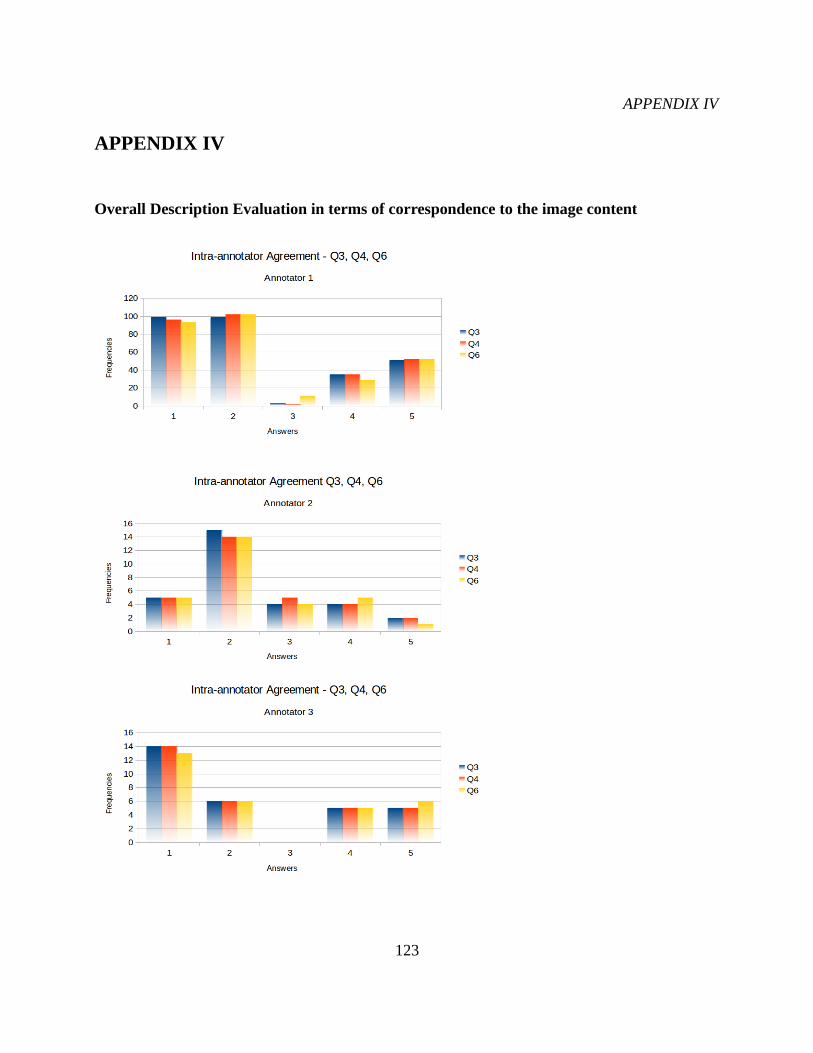
APPENDIX IV

APPENDIX IV

Overall Description Evaluation in terms of correspondence to the image content

123

APPENDIX IV

Overall Description Evaluation

124

APPENDIX IV

Human Activity Recognition

125

APPENDIX IV

Subject & Object Recognition

126

APPENDIX IV

Overall Language Evaluation - Language Fluency

127

APPENDIX IV

Grammatical Errors

128

APPENDIX IV

129

APPENDIX IV

Lexical Errors

130

APPENDIX IV

131

APPENDIX IV

Sentence Completeness

132

APPENDIX IV

Sentence Clarity - Meaning Adequacy

133