imaging fast moving objects with application to satellite ... fileimaging fast moving objects with...

Imaging fast moving objectswith application to satellite imaging

George PapanicolaouStanford University

Meeting in honor of Patrick Joly

August 29, 2017

With: J. Fournier, J. Garnier, C. Tsogka and L. Borcea, K. Solna,

G. Papanicolaou, Joly-60 Imaging 1/20

How did this research project start

Use passive sensor arrays as a way to image (a) through stronglyinhomogeneous media, and (b) with independent, asynchronous, andunknown (often opportunistic) illumination.

1. Started in seismic imaging for hydrocarbons around 2005 but has alonger history. Around 2010 passive synthetic aperture radar (SAR)begun to be used for imaging ground reflectivities usingopportunistic illumination, either ground based on from satellites1.

2. We decided to consider passive SAR to image satellites. The passiverecording platform(s) is (are) to fly above the atmosphere (at about20 km or more), the illumination coming from the ground. Thesatellite is low flying (at about 300-1000 km), and is rapidly moving(to remain in orbit).

1Passive Imaging with Ambient Noise, Garnier and Papanicolaou, Cambridge University Press 2016


What can theory and numerical simulations do

1. The effect of atmospheric inhomogeneities is minimized withhigh-flying, passive receivers (Garnier+P, SIIMS 2014 and 2015).

2. Focus the theory on resolution analysis. Analytically challenging butcan be done from first principles.

3. Compare ground-based matched-filter imaging (currently in use) and(the proposed) passive receiver, correlation-based imaging.

4. Main result: In the X-Band (10 GHz) regime, and with six to ninerecording platforms (ground-based or drones) over a 200× 200kilometer region the satellite position and velocity image resolutionsare comparable for the two modalities, can be quantified very well,and are close to optimal, down to centimeter level (with awavelength of 3cm).


Imaging with passive auxiliary arrays schematic

VT

~e3

~e2

~e3

YT

HT

a

a

Receivers

R1

R2

R3

XE

EmitterScatterer

Legend:

XR3

Configuration with receivers above ground


Scaterring by a moving object

A (point) transmitter at XE emits a short pulse f(t). The total fieldu(t,x) solves

1

c2(t,x)

∂2u

∂t2− ∆u = f(t)δ(x−XE), (1)

with a localized perturbation ρT centered at the moving target XT (t),

1

c2(t,x)=

1

c2o

(1 + ρT

(x−XT (t)

)).

The incident field u(0)(t,x) is

u(0)(t,x) =1

4π |x−XE|f(t−

|x−XE|

co

). (2)


The scattered field

In the Born approximation the scattered field is given by

u(1)(t,x) = −1

c2o

∫t0

dτ

∫dyG(t− τ,x,y)ρT (y −XT (τ))

∂2

∂τ2u(0)(τ,y).

For a point-like scatterer,

u(1)(t,x) = −ρ

c2o

∫t0

dτG(t− τ,x,XT (τ))∂2

∂τ2u(0)(τ,y) |y=XT (τ),

where ρ =∫ρT (x)dx is the reflectivity of the target. Using u(0) and

integrating by parts twice:

u(1)(t,x) = −ρ

c2o

∫t0

dτ

∫τ0

dτ ′f ′′(τ ′)G(τ−τ ′,XT (τ),XE)G(t−τ,x,XT (τ)).

Therefore the scattered field at the receiver at x = XR is

us,R(t) = −ρ

c2o

∫t0

dτ1

4π|XT (τ) −XE|f ′′(τ−

|XT (τ) −XE|

co

)× 1

4π|XR −XT (τ)|δ(t− τ−

|XR −XT (τ)|

co

).


The scattered field, continued

If we introduce

Φ(τ; t) = t− τ−|YT −XR + τVT |

co,

then we have

δ [Φ(τ; t)] =δ[τ− τ(t)]

|∂τΦ(τ(t); t)|,

with τ(t) the unique zero of τ→ Φ(τ; t) in (0, t). DenotingD(t) = YT −XR + tVT , We find that τ(t) is given by

τ(t) = t−|D(t)|

co(1 −

∣∣VT

co

∣∣2)√1 −

∣∣∣∣VTco∣∣∣∣2 + (VT

co· D(t)

|D(t)|

)2

−VTco· D(t)

|D(t)|

.

(3)Using this in us,R(t) we get the (model) signal recorded at the receiver

us,R(t) = −ρf ′′(τ(t) − |XT (τ(t))−XE|

co

)(4π)2c2o|XT (τ(t)) −XE||XR −XT (τ(t))|

∣∣∣1 + VT

co· D(τ(t))|D(τ(t))|

∣∣∣ .(4)


What is the imaging problem

• We record us,R(t) at various receiver locations XR. These locations(not moving for simplicity here) are assumed known.

• The source location must be know in matched field imaging. It neednot be known for correlation based imaging.

• We want to find (estimate) the target location YT and velocity VT .This is a point in six dimensions in general. For satellites it can bereduced to five with a ”tangential” VT .

How are we to do this? We construct Imaging functions.


Imaging functions: Matched field

The idea behind the matched-filter imaging function is that we want tomatch the received signal with the emitted pulse. The matching processinvolves the assumed initial position and speed of the object (Y ,V ), andthis matching can be shown to be maximal at the true position (YT ,VT ).The matching process takes into account a (derived) Dopplercompensation factor γs(X,V ,XR),

IMF(Y ,V ) =1

NE

NE∑j=1

IMFj (Y + V Sj,V ),

IMFj (X,V ) =

1

N

N∑R=1

∫f(γs(X,V ,XR)

(t−

|X −XR|

co

)−

|X −XE|

co

)us,R(Sj + t)dt

This imaging function requires knowledge of the transmitter and receiverpositions XE and XR. We also need to know the pulse profile f. Onewants to image a region around some point YT , so the j-th scatteredsignal needs only to be recorded for a short time around 2|YT −XE|/co.


Imaging functions: Cross correlations

We cross correlate the scattered signals recorded by pairs of receivers andmigrate them with the appropriate Doppler compensation factors,

ICC(Y ,V ) =1

NE

NE∑j=1

ICCj (Y + V Sj,V ), (5)

ICCj (X,V ) =1

N2

N∑R,R′=1

∫us,R

(Sj +

|X −XR|

co+

t+ |X−XE|

co

γs(X,V ,XR)

)

× us,R′

(Sj +

|X −XR′ |

co+

t+ |X−XE|

co

γs(X,V ,XR′)

)dt. (6)

Bow it is not necessary to know the pulse profile f which could bedifferent from one emission to another one. It is not necessary either toknow the emission times with accuracy. But we need to record the wholetrain of scattered signals. Moreover correlation-based imaging has beenshown to be robust to medium fluctuations when in a suitable imagingconfiguration2.

2Garnier+P, CUP, 2016


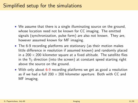
Simplified setup for the simulations

• We assume that there is a single illuminating source on the ground,whose location need not be known for CC imaging. The emittedsignals (synchronization, pulse form) are also not known. They are,however assumed known for MF imaging.

• The 6-9 recording platforms are stationary (as their motion makeslittle difference in resolution if assumed known) and randomly placedin a 200× 200 kilometer square at a fixed altitude. The satellite fliesin the Y2 direction (into the screen) at constant speed starting rightabove the source on the ground.

• With only about 6-9 recording platforms we get as good a resolutionas if we had a full 200× 200 kilometer aperture. Both with CC andMF imaging.


Satellite imaging with (passive) X-band SAR

System ParametersCentral Frequency f0 9.6 GHzBandwidth B 622 MHzNumber of Frequencies in Bandwidth Nf 515Slow-time Sampling ∆s 0.015 sWave Speed co 3× 108 m/sCentral Wavelength λo 3.12 cmAltitude of Satellite H 500 kmSpeed of Satellite VT 7,610.6 m/sAltitude of Drone h 20 kmVelocity of Drone VR 222.2 m/s (800 km/hr)

Parameters for modeling SAR imagining of a satellite with passive SARon a platform above the atmosphere and microwave sources on theground.


Resolution results from the simulation

• There are five ”parameters” to be imaged: The three components ofthe satellite (say its initial) location and the (assumed) twocomponents of its speed. We actually include vertical speed as wellsince it is needed when dealing larger size space objects.

• The passive SAR platform covers a distance of 5 km, in 22.5 secs.During this time the satellite covers a distance of 171 km. These arethe recording windows used.


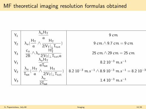
MF theoretical imaging resolution formulas obtained

Y1λoHT

a9 cm

Y2 λo(HT

a∧

HT

2|VT |⊥Ttot) 9 cm∧ 9.7 cm = 9 cm

Y3co

2B∧ λo

H2T

2|VT |⊥Ttota25 cm∧ 29 cm = 25 cm

V1λoHT

aTtot8.2 10−3 m.s−1

V2λo

Ttot(HT

a∧

HT

2|VT |⊥Ttot) 8.2 10−3 m.s−1 ∧ 8.9 10−3 m.s−1 = 8.2 10−3 m.s−1

V3λo

2Ttot1.4 10−3 m.s−1


CC theoretical imaging resolution formulas obtained

Y⊥λoHT

a1.4 10−3m

Y3 λo

(H2T

a2∧

2H2T

aVTTtot

)9.0 10−2m. ∧ 1.2m

V⊥λoHT

aTtot8.2 10−3m.s−1

V3λo

Ttot

(H2T

a2∧

2H2T

aVTTtot

)2.5 10−2m.s−1 ∧ 1.1 10−1m.s−1


MF and CC horizontal-horizontal (Y1, Y2) resolutions

MF CCTtot=

22.5

sTtot=

11.2

5s

Images with MF and CC in the (Y1, Y2) plane. The units are in m. Thesatellite velocity is VT = 7610m/s. The first row is for recording durationTtot = 11.25s and the second for Ttot = 22.5s.


MF and CC horizontal-vertical (Y1, Y3) resolutions

MF CCTtot=

22.5

sTtot=

11.2

5s

Images with MF and CC in the plane (Y1, Y3). The units are in m. Thesatellite velocity is VT = 7610m/s. The first row is for recording durationTtot = 11.25s and the second for Ttot = 22.5s.


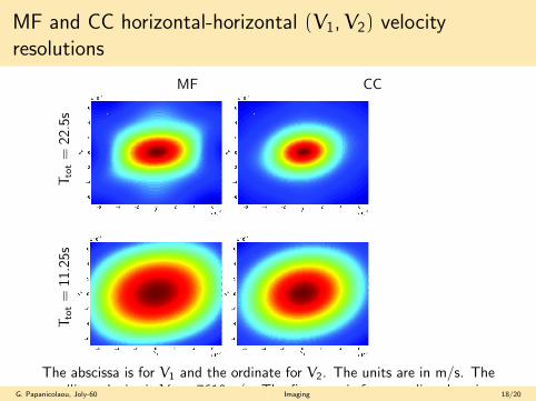
MF and CC horizontal-horizontal (V1,V2) velocityresolutions

MF CC

Ttot=

22.5

sTtot=

11.2

5s

The abscissa is for V1 and the ordinate for V2. The units are in m/s. Thesatellite velocity is VT = 7610m/s. The first row is for recording durationTtot = 11.25s and the second for Ttot = 22.5s.


MF and CC horizontal-vertical (V1,V3) velocity resolution

MF CCTtot=

22.5

sTtot=

11.2

5s

The abscissa is for V1 and the ordinate for V3. The units are in m/s. Thesatellite velocity is VT = 7610m/s. The first row is for recording durationTtot = 11.25s and the second for Ttot = 22.5s.


Conclusions

• We have shown that passive SAR imaging of satellites can be donewith a resolution that is essentially the optimal one, properlyinterpreted, when using a suitably adjusted imaging function toaccount for rapid target motion. The resolution theory is challengingbut essentially complete now, both for CC and MF (currently used)imaging. CC and MF imaging resolutions are comparable for multiplereceivers (continuum approximation) and ”large” apertures3.

• CC imaging is robust to atmospheric inhomogeneities when forexample the satellite is low in the horizon and signal paths are longinside the atmosphere. Numerical simulations to explore this need tobe done and are challenging.

• Need to address: Synchronization issues, SNR issues, finite sizesatellite effects, including rotation, swarms of debris, global smallscale tracking .... Sparse Arrays ...

3Two papers in the SIAM J. on Imaging Science, 2017


imaging fast moving objects with application to satellite ... fileimaging fast moving objects with...

Documents