imaging microvascular changes associated with neurological ... · ii imaging microvascular changes...
TRANSCRIPT
Imaging Microvascular Changes Associated with Neurological Diseases
by
Brige Paul Chugh
A thesis submitted in conformity with the requirements for the degree of Doctor of Philosophy
Medical Biophysics University of Toronto
© Copyright by Brige Paul Chugh 2012
ii
Imaging Microvascular Changes Associated with Neurological
Diseases
Brige Paul Chugh
Doctor of Philosophy
Medical Biophysics
University of Toronto
2012
Abstract
Microvascular lesions of the brain are observed in numerous pathological conditions including
Alzheimer's disease (AD). Regional patterns of microvascular abnormality can be characterized
using current neuroimaging technologies. When applied to mouse models of human disease,
these technologies reveal cerebral vascular patterns and help uncover genotype-to-phenotype
relationships. This thesis focuses on the development and testing of techniques for measuring
two perfusion-related metrics in mouse brain regions, namely, cerebral blood volume (CBV) and
cerebral blood flow (CBF) using micro-computed tomography (micro-CT) and arterial spin
labeling (ASL), respectively. The main developments for measurement of CBV have included:
refinements to micro-CT specimen preparation; registration of micro-CT images to an MRI
anatomical brain atlas; and masking of major vessels to calculate small-vessel CBV (sv-CBV).
The development of this micro-CT technique provided reference values of CBV over
neuroanatomical brain regions in wildtype mice. A separate study was conducted to assess
regional sv-CBV in a mouse model of AD; this study was motivated by the prevalence of
iii
microvascular lesions in patients who suffer from AD. Significant regional differences in sv-
CBV were found between AD-afflicted mice and controls. The main developments for
measurement of CBF have included: design and implementation of accurate ASL slice
positioning and optimization of inversion efficiency parameters. The development of this ASL
technique provided reference values of CBF over neuroanatomical brain regions in wildtype
mice. These techniques for measuring CBV and CBF over mouse brain regions could lead to
improved characterization of vascularity in models of neurological diseases.

iv
Acknowledgments
I thank my parents for their unwavering love, support and encouragement.
I thank my supervisor, Dr. John Sled, for providing this excellent educational opportunity and for
his expert guidance. I most appreciate his creative and skillful approach to problem solving.
I am grateful to Dr. Mark Henkelman, Dr. Jonathan Bishop, Dr. Jason Lerch, Dr. Bob Harrison,
Dr. Martin Pienkowski, Dr. Jian Wu, Dr. Lisa Yu and Dr. Yu-Qing Zhou for their major
contributions to the thesis manuscripts. I thank Joseph Steinman for his valuable editorial advice.
I appreciate the contributions of the following people in making the PhD project a success: Lily
Morikawa, Marvin Estrada, Michael Wong, Jun Dazai, Xiaoli Zhang, Shoshana Spring, Christine
Laliberté, Dr. Brian Nieman, Dr. Jacob Ellegood, Dr. Revital Manor, Dr. Bojana Stefanovic, Dr.
Jan Scholz and Matthijs van Eede.
I thank each of my committee members, namely, Dr. Simon Graham, Dr. Bob Harrison, Dr. John
Sled and Dr. Mark Henkelman for providing me with expert guidance and helping me work
through the challenges encountered in the PhD program to ensure that the project stayed on
course.

v
Attributions
Beyond sources already cited in the body of the thesis, I would like to acknowledge the
following specific attributions:
1- Dr. John G. Sled authored the automated vessel tracking software;
2- Dr. Jason P. Lerch authored the cortical surface plotting tools and non-linear registration
pipelines;
3- Dr. Lisa X. Yu collaborated with the author of this thesis to perform the surgical procedures
described in chapter 2 and 3;
4- Dr. Jian Wu, under the guidance of Dr. Yu-Qing Zhou, performed the pulsed-wave Doppler
ultrasound measurements described in chapter 4;
5- All histology protocols including immunohistochemistry and slide scanning were performed
by staff at the Centre for Modeling Human Disease (Pathology Core) under the supervision of
Lily Morikawa;
6- The TgCRND8 mouse colony, described in chapter 3, was managed by staff at the Toronto
Centre for Phenogenomics, with original mouse breeding pairs obtained from Dr. Sheena
Josselyn with the permission of Dr. Peter St. George-Hyslop. Genotyping was performed by the
Centre for Applied Genomics of the Hospital for Sick Children.

vi
Table of Contents
Abstract ii
Acknowledgments iv
Attributions v
List of Tables ix
List of Figures x
List of Abbreviations xi
Introduction and Overview 1-24
1.1 Advantages of studying mouse models 1
1.2 General principles for measuring CBV and CBF 3
1.3 Measurement of CBF 6
1.4 Measurement of CBV 16
1.5 CBV and CBF in the normal state 20
1.6 Abnormal CBV and CBF in Alzheimer’s disease 21
1.7 Structure and organization of this thesis 24
vii
Thesis Manuscripts 25-76
Chapter 2: Measurement of Cerebral Blood Volume in Mouse Brain Regions using
Micro-computed Tomography
25
2.1 Foreword 25
2.2 Introduction 25
2.3 Materials and methods 26
2.4 Results 34
2.5 Discussion 39
Chapter 3: High Resolution MRI and Micro-CT Imaging show Microvascular and
Neuroanatomical Changes in a Mouse Model of Alzheimer’s Disease
43
3.1 Foreword 43
3.2 Introduction 43
3.3 Materials and methods 45
3.4 Results and Discussion 49
3.5 Conclusion 57
Chapter 4: Robust Method for 3D Arterial Spin Labeling in Mice 58
4.1 Foreword 58
4.2 Introduction 58

viii
4.3 Materials and methods 60
4.4 Results 70
4.5 Discussion 73
Discussion and Conclusion 77-84
5.1 Summary 77
5.2 Further technical considerations 78
5.3 Future directions 84
Bibliography 85
ix
List of Tables
1.1 Comparison of sample tracers used for CBF measurements 7
1.2 Abnormalities in resting state CBV and CBF in APP mouse models 23
2.1 Total CBV and sv-CBV values for thirteen brain regions and the total brain 36
3.1 Regional values of brain volume and sv-CBV 51
3.2 Regional plaque load 56
4.1 Regional values of T1 and CBF 72
x
List of Figures
1.1 Schematic of spin inversion in CASL experiments 16
2.1 Illustration of a representative inverted maximum intensity projection of a
micro-CT image
28
2.2 The mid-sagittal section of a micro-CT image 31
2.3 CBV maps over the surface of the cerebral cortex, averaged over nine mice 33
2.4 Representation of 13 regions featured in Table 2.1 37
2.5 Comparison of mean sv-CBV for regions in left versus right hemisphere 38
2.6 Plot of mean CBV versus normalized distance from the inner surface of the
cortex toward to outer surface
39
3.1 Regional differences in brain volume between TgCRND8 and control mice 50
3.2 Variation of sv-CBV illustrated over right and left cortical surface maps 53
3.3 Amyloid plaques were observed in TgCRND8 mice 55
4.1 Illustration of process of correcting for MT 61
4.2 Regions of interest in MRI atlas with corresponding mean CBF map 67
4.3 Bilateral symmetry of CBF for nine brain regions 68
4.4 Dependence of velocity-weighted inversion efficiency for an am-CASL
experiment
69
4.5 Power analysis for difference in hippocampal CBF 71
5.1 Regional comparison of svCBV for wildtype mice from chapter 2 and 3 81
5.2 Intensity-based clustering of amyloid, Microfil and background pixels 82
xi
List of Abbreviations
2D two-dimensional
3D three-dimensional
ACA anterior cerebral artery
AD Alzheimer's disease
am-CASL amplitude-modulated continuous arterial spin labeling
ANOVA analysis of variance
APP amyloid precursor protein
ASL arterial spin labeling
B1 radio-frequency amplitude
BBB blood brain barrier
C57BL/6 identification for a common inbred mouse strain
CAA cerebral amyloid angiopathy
CASL continuous arterial spin labeling
CBF cerebral blood flow
CBV cerebral blood volume
COV coefficient of variation

xii
CPP cerebral perfusion pressure
CPV cerebral plasma volume
CRCV cerebral red cell volume
DNA deoxyribonucleic acid
ETL echo train length
fm modulation frequency
FOV field-of-view
G gradient strength
Hct hematocrit
IP intraperitoneal
micro-CT micro-computed tomography
MCA middle cerebral artery
MRI magnetic resonance imaging
MT magnetization transfer
NEX number of excitations
PASL pulsed arterial spin labeling
PBS phosphate buffered saline
xiii
pCASL pseudo-continuous arterial spin labeling
PECAM-1 platelet endothelial cell adhesion molecule-1
PET positron emission tomography
PS permeability surface area product
RF radio frequency
SAR specific absorption rate
SEM standard error of the mean
SNR signal-to-noise-ratio
SPECT single photon emission computed tomography
SSS superior sagittal sinus
sv-CBV small-vessel cerebral blood volume
T unit of magnetic field strength: tesla
TE echo time
TR repetition time
T1 time constant for longitudinal relaxation
T1SAT time constant for longitudinal relaxation, enhanced by magnetization transfer
T2 time constant for transverse relaxation

xiv
T2*
time constant for decay of transverse magnetization, including both spin-spin
relaxation and relaxation due to magnetic filed inhomogeneity
TgCRND8 identification code for a mouse model of Alzheimer's disease

1
Chapter 1 Introduction and Overview
This thesis focuses on the development and testing of techniques for measuring two perfusion-
related metrics to quantify regional patterns of cerebral microvascular abnormalities of
genetically modified mice. The proposed metrics, namely, cerebral blood volume (CBV) and
cerebral blood flow (CBF), are measured using state-of-the-art imaging technologies. The
background to this work is introduced here, while description of the experimental design and
findings are detailed in the main body of the thesis, comprising three manuscripts.
There are two main goals of this introduction, namely, 1-to place the techniques developed in
this thesis within the broader context of the available methods for characterizing microvascular
abnormalities; and 2-to provide a rationale for the developments and applications described in
the body of this thesis.
For ease of discussion, this introduction has been divided into seven sections each of which deals
with a relevant theme. We start by considering the benefits of using mouse models in our study.
In the context of mouse imaging, the principles for measuring CBV and CBF are outlined. The
normal state of CBV and CBF is discussed, before considering cerebro-vascular abnormalities in
Alzheimer’s disease. This is followed by outlining the structure and organization of this thesis.
1.1 Advantages of studying mouse models
There has been rapid growth in our knowledge of the 20,000-25,000 protein-coding genes(1) that
comprise the human genome and in our technological ability to manipulate homologous genes in
genetically engineered mouse models. Each of the following subsections describes a distinct
advantage of using mice as mammalian models for the study of genetics.
1.1.1 Humans and mice still possess many common traits after 75 million years of evolution
The genetic pathways in mice are very similar to those of humans. There is a very high
probability, approximately 99%, that a given mouse gene has a homologue in the human genome

2
(2). This leads to many similarities in the observable traits of the two species. Despite obvious
differences in brain function, mice and humans have a surprisingly similar spatial arrangement of
brain regions. It has long been recognized that the cerebral vasculature in the mouse has a similar
anatomical arrangement to that in humans(3).
1.1.2 Genetically identical mice of various strains are available
Gregor Mendel published the laws of inheritance in 1866 based on observations made in pea
plant hybridization experiments. Long before Mendel's work, it was known that certain strains of
mice spontaneously produced coat-colours that were different than the norm. By the 1700s,
mouse fanciers in Japan and China had domesticated many varieties as pets while Europeans
subsequently imported favorites and bred them to local mice, thereby creating progenitors of
modern laboratory mice. The laws of Mendelian inheritance were demonstrated on mouse coat
colours, which extended genetic principles from pea plants to mammals. Subsequently, mating
programs were established, resulting in many of the modern well-known inbred strains(2). These
inbred strains represent an unlimited family of genetically identical individuals and provide an
opportunity to perform experiments on very similar phenotypes without much intrinsic
variability. Various genetic engineering techniques may be employed such as the inactivation of
genes to create knock-out mouse models, introduction of genes from another species (knock-in
models) and inactivation of a gene in a confined spatial or temporal region (conditional
knockouts).
1.1.3 The complexity of mammalian biology can be studied from a system-wide perspective
The completion of the human genome project involved decoding a database consisting of 3.3
billion base pairs of deoxyribonucleic acid (DNA), known as the human genome. As a next step,
if we can learn how the genome results in observable human characteristics, known as the
phenotype, then this would lead to a vastly improved understanding of our biological makeup.
Thus, a current challenge facing biologists is to uncover genotype-to-phenotype relationships.
This is complicated, however, by the fact that single gene modifications seldom result in a single
phenotypic change. In fact, single gene changes typically give rise to multiple and often diverse
phenotypes. Furthermore, many common diseases affecting humans, including Alzheimer’s
disease, involve multiple genes.

3
Therefore, a paradigm known as systems biology is being developed to focus on how complex
properties of a system emerge from the interactions between simpler components(4). In this
paradigm, genotype-to-phenotype relationships are understood from a holistic perspective by
associating genetic variants with traits observed from a whole organ or whole organism system-
wide perspective. Since the genomes of several strains of mice have also been sequenced, mouse
models can contribute to this approach by permitting genotype-to-phenotype relationships to be
uncovered. This can be achieved by genetically modifying some members of an inbred strain of
mice and looking for associated changes in the phenotype relative to unmodified members.
Two of the key technologies contributing to mammalian phenotyping are magnetic resonance
imaging (MRI) and micro-computed tomography (micro-CT)(4). The application of imaging
technologies provides numerous benefits for the discovery of genotype-to-phenotype
relationships. Imaging can go beyond simply revealing anatomical differences, as it can also
provide glimpses of physiological phenotypes such as those associated with brain perfusion.
1.2 General principles for measuring CBV and CBF
The term perfusion describes the delivery of arterial blood to the capillary bed, which involves
transport of oxygen, glucose and other nutrients from blood to tissue. Techniques for measuring
perfusion-related parameters have and will continue to be useful in neuroscience. These
techniques provide the ability to chart out microvascular structure over brain regions and to
detect deviations from normal cerebral blood flow. The following sections define the principles
for measurement of two of the most useful metrics for characterizing perfusion.
1.2.1 Definitions
In quantitative brain imaging, the key perfusion-related parameters describing the vascular
structure and the rate of perfusion are cerebral blood volume (CBV) and cerebral blood flow
(CBF), respectively.
CBV is defined as the total volume of blood per unit volume of brain tissue(5) and is
conventionally expressed in percentage units. CBV values are similar between species but
heterogeneous over regions, with human values ranging from 2.7% in white matter to 8.6% in
4
occipital cortex(6). CBV depends on both vessel density and diameter and is, thus, sensitive to
the distribution of vessel types. On average and under in vivo conditions, the approximate
breakdown of CBV is estimated as follows: 10% is associated with arterial blood, 20% with
capillary blood and 70% with venous blood(7). Estimates for the compartmentalization of CBV
within the microvasculature vary; for example, one report provides a breakdown of 20%
arteriolar, 50% capillary and 30% venular(8) and another report provides 21% arteriolar, 33%
capillary and 46% venular(9). Several techniques for measuring CBV are covered in section 1.4.
CBF is defined as the volume of arterial blood (in mL) delivered to the capillary bed of 100g of
brain tissue per minute. This definition assumes that arterial blood is delivered to the capillary
bed such that the constituent components of blood, including oxygen and nutrients, are deposited
in the tissue element of interest; this contrasts with arterial blood flow that transits through a
tissue element on route to another destination, without locally depositing its constituent
components(10). CBF varies substantially between species, with healthy human CBF at about 50
mL/100g/min, while mouse CBF has been typically found to be 150 mL/100g/min or higher. The
scaling of units to 100g of brain tissue is a conventional practice, though the quantity of brain
tissue may also be expressed in volume units, in which case CBF would have the dimensions of a
rate constant. This dimensional analysis highlights the role of CBF in delivery of metabolic
substrates and clearance of metabolic products. Specifically, the rate of delivery of any substrate
to the tissue is the product of CBF and the arterial concentration of the substrate(8).
There are several techniques for measuring CBF over neuroanatomical brain regions, with some
of the key imaging methods discussed in section 1.2.2. CBF is heterogeneous under normal
circumstances, typically varying by at least a factor of four over mouse brain regions(11). This
variation may be attributed to differences in metabolic demand of tissues. In fact, CBF has been
shown under normal conditions to be proportional to the measured metabolic rate(12).
This thesis focuses on the mapping of CBV and CBF over mouse brain regions, which is of
particular interest for delineating phenotypes of models of neurological diseases, such as
Alzheimer's disease(13). As explained in the following subsections, there are numerous
considerations in mapping these metrics in the brain.

5
1.2.2 General tracer kinetic model
Principles for measurement of CBF may be described by the following linear systems model(8;
14), which describes the kinetics of a tracer as it travels from feeding arterial source to the
receiving tissue region:
)]([)()( trftCtC AT [1.1]
f
tr
0
)( , [1.2]
where CA(t) is the tracer concentration in the arterial blood (also known as the arterial input
function), CT(t) is the tracer concentration in tissue, f is cerebral blood flow, λ is the partition
coefficient, r(t) is the residue function, while denotes the convolution operation.
The partition coefficient is defined in a steady-state tracer experiment as the ratio of tracer
concentration in tissue to that in the artery. Specifically, if CA(t) is constant, i.e. 0)( CtCA , for a
lengthy period of time, then 0/)( CCT . The partition coefficient is also known as the
volume of distribution of the tracer because it is a generalization of CBV to include cases where
the tracer is diffusible outside of the vasculature. Tracers can be categorized based on their λ,
with diffusible tracers having λ~1 and intravascular tracers having λ~CBV.
The residue function is the probability that a particle of the tracer that entered a volume element
(i.e. voxel) of the region of interest at t=0 is still there at time t. In other words, the transport and
distribution of the tracer are characterized by r(t), which is a monotonically decreasing function
with initial value 1. The area under the residue function, as described in equation [1.2], is
referred to as the mean transit time (τ) and represents the fundamental time constant governing
the kinetics of the tracer. It is clear from equation [1.2] that the class of tracer selected, which
affects λ, can strongly affect the time constant for the experiment.
The general model described by equations [1.1] and [1.2] holds provided that two assumptions
are true for the course of the experiment, namely: 1- the brain is in steady state with CBF
constant; and 2-the tracer is metabolically inert(8).
6
1.3 Measurement of CBF
To apply the general tracer kinetic model for measurement of CBF using neuroimaging
technologies, it is necessary to relate the signal associated with the tracer, as measured by the
imaging modality, to the concentration of the tracer, i.e. CA(t) and CT(t). In the following
sections, techniques for measuring CBF are compared based on different tracer properties and a
discussion is provided on challenges of applications to mice.
1.3.1 Tracers for the measurement of CBF
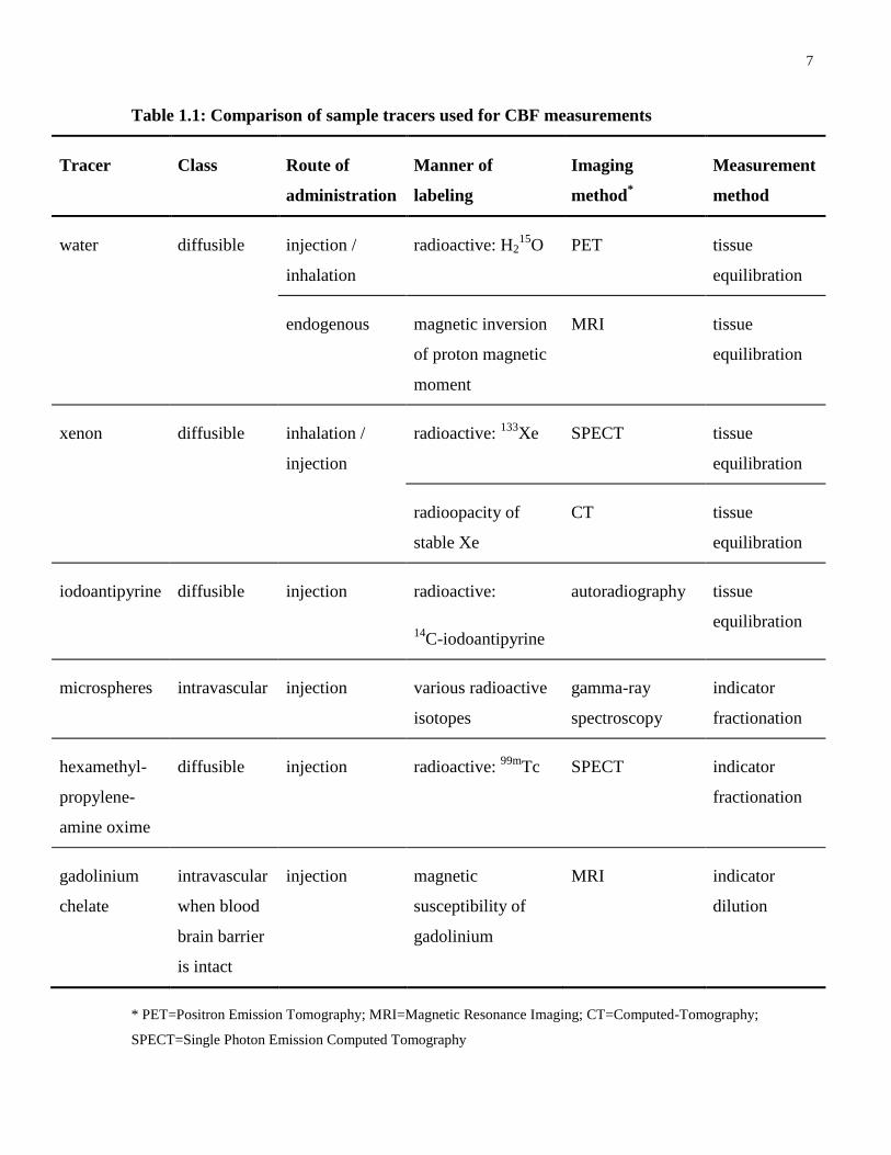
Several tracers used for CBF quantification are listed in Table 1.1 along with their key
properties. Tracers for CBF measurement can be labeled in various ways so as to be detectable
by neuroimaging modalities. For example, water can be radioactively labeled to be detectable by
positron emission tomography (PET) or can be magnetically labeled for detection by arterial spin
labeling (ASL), an MRI technique. Since water is a diffusible tracer and has the same partition
coefficient irrespective of the labeling method, both PET and ASL methods share many common
properties. Thus, it is useful to think about CBF measurement from the point of view of the
tracer selected.
The pioneering method for measuring total blood flow through the heart or lungs was the Fick
principle, enunciated by Adolf Fick in 1870. This principle states that the quantity of a tracer
taken up by an organ per unit time is equal to the product of blood flow through that organ and
the tracer concentration difference between artery and vein(15; 16). A breakthrough in cerebro-
vascular research followed with the advent of the “Kety method”, also known as the “tissue
uptake” method, devised by Kety and Schmidt in 1948, which adapted Fick’s principle to
measure whole brain CBF in humans using inhaled nitrous oxide, a diffusible tracer. Due to the
non-availability of tomographic neuroimaging methods to provide voxel-wise tissue
concentration, Kety and Schmidt invasively sampled arterial and venous blood to measure the
concentration-time curves for nitrous oxide over a ten minute time period, long enough for the
nitrous oxide to reach equilibrium within the brain. Whole brain CBF was estimated to be 54±12
ml/100g/min, based on data from 14 healthy young males(17).
7
Table 1.1: Comparison of sample tracers used for CBF measurements
Tracer Class Route of
administration
Manner of
labeling
Imaging
method*
Measurement
method
water diffusible injection /
inhalation
radioactive: H215
O PET tissue
equilibration
endogenous magnetic inversion
of proton magnetic
moment
MRI tissue
equilibration
xenon diffusible inhalation /
injection
radioactive: 133
Xe SPECT tissue
equilibration
radioopacity of
stable Xe
CT tissue
equilibration
iodoantipyrine diffusible injection radioactive:
14C-iodoantipyrine
autoradiography tissue
equilibration
microspheres intravascular injection various radioactive
isotopes
gamma-ray
spectroscopy
indicator
fractionation
hexamethyl-
propylene-
amine oxime
diffusible injection radioactive: 99m
Tc SPECT indicator
fractionation
gadolinium
chelate
intravascular
when blood
brain barrier
is intact
injection magnetic
susceptibility of
gadolinium
MRI indicator
dilution
* PET=Positron Emission Tomography; MRI=Magnetic Resonance Imaging; CT=Computed-Tomography;
SPECT=Single Photon Emission Computed Tomography
8
Kety’s model can be considered a special case of the more general kinetic model described by
equations [1.1] and [1.2] with an assumed residue function of )/exp()( ttr . This residue
function is equivalent to assuming that the nitrous oxide reaches a rapid equilibrium between
tissue and blood within a single well-mixed compartment(8). Several methods of CBF
measurement assume this residue function and are collectively known as “tissue equilibration”
techniques. As listed in Table 1.1, water, xenon and iodoantipyrine are examples of diffusible
tracers that are well suited to meet the requirements of the tissue equilibration method(7; 18).
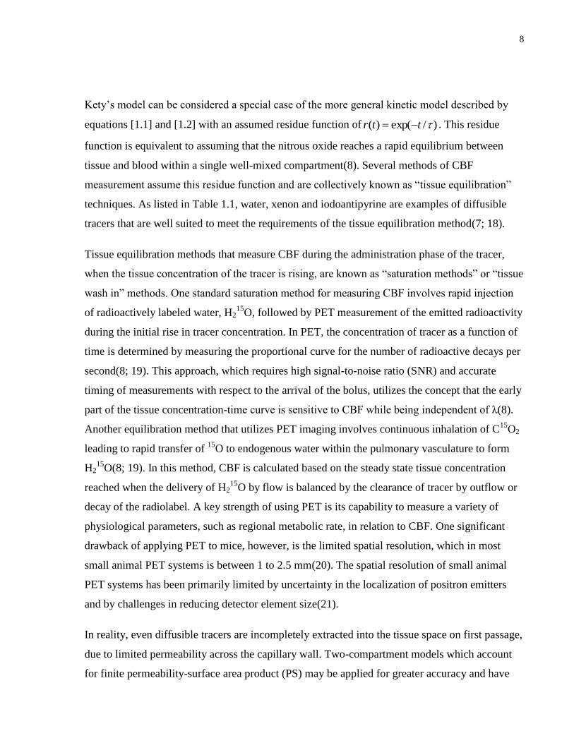
Tissue equilibration methods that measure CBF during the administration phase of the tracer,
when the tissue concentration of the tracer is rising, are known as “saturation methods” or “tissue
wash in” methods. One standard saturation method for measuring CBF involves rapid injection
of radioactively labeled water, H215
O, followed by PET measurement of the emitted radioactivity
during the initial rise in tracer concentration. In PET, the concentration of tracer as a function of
time is determined by measuring the proportional curve for the number of radioactive decays per
second(8; 19). This approach, which requires high signal-to-noise ratio (SNR) and accurate
timing of measurements with respect to the arrival of the bolus, utilizes the concept that the early
part of the tissue concentration-time curve is sensitive to CBF while being independent of λ(8).
Another equilibration method that utilizes PET imaging involves continuous inhalation of C15
O2
leading to rapid transfer of 15
O to endogenous water within the pulmonary vasculature to form
H215
O(8; 19). In this method, CBF is calculated based on the steady state tissue concentration
reached when the delivery of H215
O by flow is balanced by the clearance of tracer by outflow or
decay of the radiolabel. A key strength of using PET is its capability to measure a variety of
physiological parameters, such as regional metabolic rate, in relation to CBF. One significant
drawback of applying PET to mice, however, is the limited spatial resolution, which in most
small animal PET systems is between 1 to 2.5 mm(20). The spatial resolution of small animal
PET systems has been primarily limited by uncertainty in the localization of positron emitters
and by challenges in reducing detector element size(21).
In reality, even diffusible tracers are incompletely extracted into the tissue space on first passage,
due to limited permeability across the capillary wall. Two-compartment models which account
for finite permeability-surface area product (PS) may be applied for greater accuracy and have
9
been seriously considered for improving the accuracy of CBF measurements using endogenous
and radiolabeled water(22; 23).
The family of CBF measurement methods based on the tissue equilibration principle also include
techniques that make a single time point measurement after the tracer concentration in tissue has
reached equilibrium. One such technique is autoradiography, which is often considered to be the
gold standard for measuring CBF over brain slices. In autoradiography, the tracer is a radio-
labeled molecule such as 14
C-iodoantipyrine, which is nearly completely extracted from the
capillaries at CBF values below 180 mL/100g/min(18). Brain concentration of the tracer is
measured by arresting the circulation and sectioning brain tissue with a cryostat, followed by
placing the slices in contact with an X-ray sensitive film. This technique is considered very
reliable because major sources of error have been thoroughly quantified(24). One drawback,
however, is that, unlike modern tomographic methods, autoradiography measures CBF in 2D.
Those tissue equilibration methods that first load up the brain with the tracer, then stop tracer
administration and finally measure CBF as the tracer clears from the tissue are known as
“clearance methods”, “desaturation methods” or “tissue washout methods”. For example, using
xenon as a tracer, the clearance curve is measured and fitted to a decaying exponential with the
time constant for clearance f/ . In the clearance method, measurements are sensitive to
both f and λ(8). One such technique is xenon computed tomography, where stable xenon
provides CT contrast by increasing x-ray attenuation. A challenge in applying this technique to
small-animals, however, is the low SNR, despite administration of high concentrations of
xenon(18).
CBF can also be measured using a tracer that gets trapped in the capillary bed or brain tissue
after initial administration, in which case the residue function is 1)( tr and the general model
becomes independent of λ. These methods, prized for their simplicity, are known as “indicator
fractionation” or “microsphere methods”, since they are modeled on the microsphere trapping
technique. Microsphere trapping involves arterial infusion of a bolus of carbonized or plastic
microspheres with mean diameter of 15µm, radiolabeled with a gamma emitter, which after
delivery to the capillary bed can be detected by differential gamma spectroscopy(7; 16; 18). As
an alternative to radiolabeling, microspheres can also be fluorescently labeled. The microspheres
are too large to fit through the capillaries so they remain lodged at the precapillary level within
10
the tissue. An integrated arterial-concentration time curve for the injected microspheres can be
measured at any convenient artery. When applied to large animals, microsphere trapping is
considered to be the gold standard for CBF measurement. When applied to small animals,
however, the large number of infused microspheres needed to obtain sufficient measurement
accuracy is believed to disturb circulatory parameters and has provided unreliable results in the
past(25).
The indicator fractionation method is also utilized with single photon emission computed
tomography (SPECT) when highly diffusible, short lived tracers get trapped in brain tissue after
an initial capillary passage and behave as “liquid microspheres”. These tracers freely pass the
blood brain barrier and undergo rapid conversion to highly bound metabolites that are retained
for several minutes, long enough for tomographic imaging. The tracer radioactivity is detected
by arrays of stationary sensors or by a gamma camera rotating around the head, and the detected
photon count rate is scaled proportionally to tracer concentration units(8; 26). Recent advances in
pin-hole camera technology provide better magnification for high resolution SPECT in mice.
However, increases in resolution are traded off with limited sensitivity since a pinhole passes
only a small fraction of the incident photons. Continued development of multiple pinholes(27)
and improved image reconstruction is making SPECT a feasible option for phenotyping mice.
It is worth noting that the specific CBF measurement method depends more on the nature of the
tracer than on the imaging modality used to detect it. Consider, for example, that using
radioactive 133
Xe and SPECT, CBF is measured by the tissue equilibration method, whereas
using 123
I- iodoamphetamine and SPECT, CBF is measured by the indicator fractionation
method.
For agents that remain intravascular in the brain during the data collection period, the so-called
“intravascular” or “blood pool” tracers, the time course of the experiment is governed by time
constant fCBV / , substantially smaller than that for diffusible tracers. For these
intravascular tracer methods, r(t) has a complex form and the shape of the tissue-concentration
curve is affected by both f and λ. Therefore, accurately measuring CBF requires high SNR and
high temporal resolution. In such cases, CBF is sometimes determined without assuming a
specific residue function, based on deconvolution of equation [1.1] using a sampled CA(t). This
method has been implemented using MRI bolus tracking, also known as dynamic contrast
11
enhanced imaging, which uses exogenous paramagnetic tracers such as gadolinium chelates. The
MRI signal depends on the effects of the contrast agent on the time constants for longitudinal
relaxation (T1) and for transverse relaxation (T2) of blood, which in turn are affected by the
distribution of magnetic susceptibility and the water exchange between intra and extravascular
spaces. Quantification is based on relating the MRI signal changes to CT(t), which depends on
either susceptibility (T2 or *
2T ) or relaxivity (T1) contrast. In the case of susceptibility contrast,
CT(t) is typically assumed to be proportional to the change in the transverse relaxation rate,
)(*
2 tR , whereas in the case of relaxivity contrast, CT(t) is typically assumed to be proportional
to change in longitudinal relaxation rate, )(1 tR . In reality, these linear relationships may be
oversimplified as the MR signal changes depend on a complex interplay of water exchange and
susceptibility-induced changes, which complicates quantitative interpretation(8; 9). Other
persistent challenges of MRI bolus tracking include high sensitivity to noise and stringent
requirements on knowledge of CA(t). However, this technique has been applied to species as
small as rats(28).
1.3.2 Developing arterial spin labeling in mice
Arterial Spin Labeling (ASL), developed in 1992(29), is an MRI technique for measuring CBF
using endogenous arterial blood water as a diffusible tracer. Due to use of water as the carrier of
contrast, ASL techniques closely parallel steady-state PET studies using H215
O. In fact, the
development of ASL was modeled on the established H215
O technique after it was realized that
developments in labeling water for use in MR angiography could be extended to CBF. As an
MRI technique, ASL can acquire CBF images in 3D and these data can be related to other MRI
data sets, such as anatomical images which provide delineation of regional boundaries. When
optimized, ASL offers better spatial resolution in CBF mapping than most other neuroimaging
techniques, including nuclear medicine methods like PET and SPECT(8). Since ASL uses
endogenous contrast, it is completely non-invasive, providing great ease of use in conducting
research on very small animals such as mice. Prior to this thesis, there had been a few studies
demonstrating 2D ASL in mice. Since this thesis develops 3D ASL for use in mice, however,
several complexities involved in transitioning from 2D to 3D ASL needed to be addressed, as
described in chapter 4.
12
ASL can be implemented in several different ways, though the following five steps can be
considered essential(8): (i)- the arterial input function, CA(t), is defined by flipping
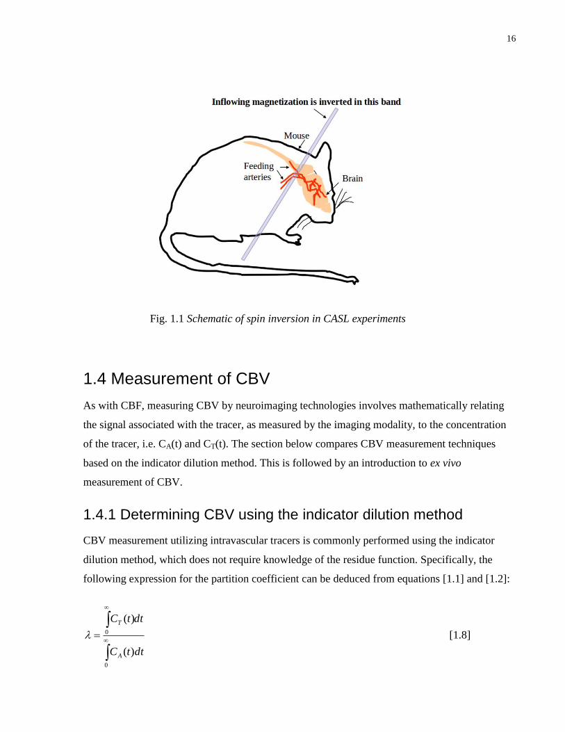
magnetization of inflowing water in arterial blood (illustrated in Fig.1.1) using 180°
radiofrequency (RF) inversion pulses; (ii)- after allowing enough time delay for the labeled
blood to irrigate the tissue of interest (a period referred to as the post-label delay) an image of the
tissue regions is acquired, which may be termed the ‘label image’; steps (i) and (ii) may be
collectively termed the ‘label experiment’; (iii)- a ‘control experiment’ is then performed where
steps (i) and (ii) are repeated, under conditions where there is effectively no inversion of arterial
blood; this leads to acquisition of a ‘control image’; (iv)- the label image is then subtracted from
the control image to produce an ASL difference image. This subtraction removes the signal of
background water spins while preserving the signal associated with the labeled arterial blood that
was delivered to the capillary bed; (v)- thus, CBF is modeled from the ASL difference image.
The first step in defining the arterial input function can be accomplished in two general ways.
In Pulsed ASL (PASL), the blood water magnetization is inverted in a thick slab located next to
the tissue slice of interest using a brief RF pulse, whereas in Continuous ASL (CASL), the
labeling is performed continuously in a plane that is distant and upstream of the imaging volume
using velocity-dependent adiabatic inversion. Although it is possible to label in a truly
continuous manner using separate decoupled RF coils for labeling and imaging, it is
conventional to also describe as CASL those experiments which use one coil for both labeling
and imaging, provided that the tissue is nearly saturated with inverted blood water at the time of
measurement. It would be more technically correct to refer to these latter experiments as almost-
continuous ASL, a practice followed by some researchers(30), although this thesis follows the
more common nomenclature. PASL, which deposits less RF power than CASL, is often favored
for human studies with strict regulations on RF power deposition. On the other hand, CASL, the
method of choice for this thesis, is preferred in small animal research where maximum SNR is
desired. To obtain high SNR, the completeness of blood water inversion, as measured by the
inversion efficiency, must be optimized in CASL experiments. Thus, a major focus of chapter 4
is the development of an optimal inversion efficiency protocol for mouse ASL.
Use of a post-label delay, as described in step (ii), serves two important purposes: 1- to clear the
intense signal from large arteries that can lead to CBF quantification errors, and 2- to ensure that

13
the labeled blood is completely delivered to all imaging voxels. For this to be effective, the
length of the selected post-label delay should be larger than the measured arterial transit
time(31). Depending on the T1 of blood and arterial transit time, it may also be important to
account for spin relaxation during the period of transit from inversion to measurement slices.
The quality of the control image generated in step (iii) is crucial to the accuracy of CBF
measurement. For an ideal control experiment, the arterial blood enters the tissue fully relaxed
and the static spins in the tissue have an identical signal to that of the label experiment. In this
case, the calculated difference image, described in step (iv), only depends on the delivered
arterial spins. Although the long RF pulse in CASL is off-resonance relative to the imaging slice,
this pulse can still produce a small direct effect on the longitudinal magnetization of the static
tissue spins and, an even more significant saturation of semisolid water protons leading to the
magnetization transfer (MT) effect. The so-called semisolid water protons, associated with
macromolecules and membranes, are not directly detectable due to their short T2, although they
influence the spin state of the liquid protons through magnetization transfer(32). Thus, it is
important that the control experiment reproduce these effects to avoid quantification errors.
Several pulse sequence methods have been devised to design a control experiment for CASL that
can accurately compensate for MT effects(33). One such method, known as amplitude-
modulated CASL (am-CASL), is explored in this thesis and has been successfully applied in
human multi-slice applications(34). In am-CASL, the RF pulse used in the control experiment
differs from that of the label experiment in that it is sinusoidally modulated at frequency fm,
creating two closely spaced inversion planes, which leads to double inversion. Provided that the
average RF power used in the control and label experiments is the same, magnetization transfer
effects can be cancelled in the difference image. A major challenge in implementing am-CASL,
however, is its sensitivity to arterial blood velocity. Thus, this technique must be carefully
calibrated for use in mice, as discussed in chapter 4.
For the final step of modeling CBF from the ASL difference image, the magnetization of the
ASL difference image is related to tracer concentration. In ASL, there are two ways for the tracer
to clear from the voxel, namely, venous outflow or longitudinal relaxation. The former is
described by the residue function, r(t), for water, while the latter by a relaxation term, m(t). In
this case, the general kinetic model is written as:
14
)]()([)()( tmtrftmtM a , [1.3]
where )(tM and )(tma represent the tissue and arterial blood magnetizations of the ASL
difference image, respectively.
In the simple case of a single well-mixed compartment, the residue function which describes the
washout of labeled spins from a voxel is a decaying exponential, )/exp()( ttr . Furthermore,
)/exp()( 1Tttm describes the fraction of magnetization remaining in the voxel after time t due
to longitudinal relaxation effects(8; 23). As described in chapter 4, strongly enhanced
longitudinal relaxation due to magnetization transfer is accounted for using a binary spin bath
model.
A mathematically equivalent description of this single-compartment model, which dates back to
work in 1992 by Detre and coworkers(29), is:
))()(()()(
1
tmtmfT
tM
dt
tMdva
, [1.4]
where )(tmv represents the venous blood magnetization of the ASL difference image and
)()(
tMtmv
.
Two-compartment CBF models, which have been reviewed elsewhere(23), have been applied in
human ASL to improve the accuracy of CBF quantification. It is not, however, well known
whether use of these more complex models is necessary for mouse ASL. Unlike single-
compartment models, two-compartment models account for restricted permeability of the vessel
wall. A specific two-compartmental formulation provided by Parkes and Tofts(23) considers the
magnetization of the ASL difference image for each tissue element as divided by the
semipermeable endothelial membrane into extravascular and blood compartments, as follows:

15
)()()( tmvtmvtM bbweew , [1.5]
where ewv and bwv are the volumes of extravascular and blood water per unit tissue volume and
)(tme and )(tmb are the magnetization differences for the extravascular water and blood
water, respectively.
Based on this formulation, the following two-compartment model equations describe the
dynamics of the blood compartment and extravascular compartments, each with their own
volumes and longitudinal relaxation times ( bT1 , eT1 , respectively):
))()(()()()())((
1
tmtmPStmftmfT
tmv
dt
tmvdbeva
b
bbwbbw
, [1.6]
))()(()())((
1
tmtmPST
tmv
dt
tmvdeb
e
eeweew
. [1.7]
For slow perfusion systems, where the measurement time is less than τ, the labeled water is
assumed to never leave the voxel, in which case 0)( tmv . On the other hand, for fast perfusion
systems, where measurement time is greater than τ, the venous blood has the same magnetization
as blood in the voxel, such that b
wbv vtmtm )()( where b
wv is the volume of water per unit
volume of blood. The former assumption is known as the slow solution whereas the latter is the
fast solution(23). Comparison is made between this two-compartment model using the fast
solution and the traditional single-compartment model, as discussed in chapter 4.
16
1.4 Measurement of CBV
As with CBF, measuring CBV by neuroimaging technologies involves mathematically relating
the signal associated with the tracer, as measured by the imaging modality, to the concentration
of the tracer, i.e. CA(t) and CT(t). The section below compares CBV measurement techniques
based on the indicator dilution method. This is followed by an introduction to ex vivo
measurement of CBV.
1.4.1 Determining CBV using the indicator dilution method
CBV measurement utilizing intravascular tracers is commonly performed using the indicator
dilution method, which does not require knowledge of the residue function. Specifically, the
following expression for the partition coefficient can be deduced from equations [1.1] and [1.2]:
0
0
)(
)(
dttC
dttC
A
T
[1.8]
Fig. 1.1 Schematic of spin inversion in CASL experiments

17
Equation [1.8] shows that λ can be determined from an experiment using any bolus of
intravascular tracer by measuring the area under the tissue-concentration time curve, with a
global scaling by the area under the arterial input function. This method does not require
knowledge of the shape of r(t) or CBF. Since intravascular tracers have a volume of
distribution CBV , this leads to a convenient method to determine CBV.
One important correction should, however, be pointed out. CBV is divided between cerebral
plasma volume (CPV) and cerebral red cell volume (CRCV) as follows(9):
CRCVCPVCBV [1.9]
Most measurements of CBV utilize tracers that distribute within the blood plasma and are, thus,
measuring CPV. If the hematocrit (Hct), namely, CBVCRCVHct / , was constant through the
vasculature, CBV could be scaled by a global measurement of hematocrit as
)1/( HctCPVCBV . However, in actuality, due to a differential in velocities of red cell and
plasma components in the microvasculature, hematocrit depends on the vessel size and, thus,
requires more complex corrections(9). Local microvascular hematocrits were reported to vary
between 0.22 and 0.35 over 44 rat brain areas in a study that autoradiographically measured both
CPV and CRCV using 125
I-labeled serum albumin and 55
Fe-labeled red blood cells(35). Thus, it
is important that hematocrit effects are considered when using plasma tracers to measure CBV,
since regions may substantially differ in their vessel size distribution.
Though equation [1.8] suggests a method for measuring CBV for a bolus with an arbitrary shape,
high temporal resolution is required to accurately sample the concentration-time curves. Relative
to dynamic methods, CBV images with greater SNR can be obtained by measuring the tracer
concentration after a steady-state has been reached. These steady-state methods have two
requirements, including: 1- the tracer is uniformly distributed throughout the vasculature, and 2-
the tracer must have a long enough half-life to provide sufficient contrast after steady state is
reached.
Numerous intravascular tracers have been employed for measurement of plasma blood volume
using steady-state methods including radionuclides, fluorescent dyes, and ultrasmall
superparamagnetic iron oxide particles.
18
An early application to mice of the steady-state indicator dilution method, known as the
radioisotope dilution method, involved use of radioiodine as an intravascular tracer and an
autogamma spectrometer for detection of radioactivity(36). This technique provided average
brain CPV of 35-40μL/g, which is equivalent to a CBV of approximately 3.5%.
A higher resolution steady-state method for measuring CBV in mice utilized fluorescent dyes
detected with multi-photon laser scanning microscopy; this application focused on the capillaries
of the left parietal cortex of seven wildtype mice and estimated CBV to be 2.2±0.2% in “the
capillary rich region of interest, avoiding large vessels”(37).
Ultrasmall superparamagnetic iron oxide particles have a long enough half-life to be useful for
steady-state CBV measurements using MRI relaxivity or susceptibility contrast(9). This method,
particularly useful for longitudinal studies, has been used in mice to provide regional maps
proportional to CBV(38), though absolute scaling of CBV is usually not provided. Scaling of
CBV requires accurate knowledge of the blood-tissue susceptibility differences when using
susceptibility contrast, while for relaxivity contrast, scaling of CBV requires reference
measurements in the vascular compartment(9). Another limitation of this method is the inability
to differentiate microvessel contributions to CBV from that of major vessels.
1.4.2 Determining CBV from ex vivo images of vascular networks
The methodologies described in section 1.4.1 estimate CBV through measurement of CPV
followed by correction using reference values of hematocrit. The main reason for taking this
indirect approach is that these methods measure CBV in vivo, where red blood cells occupy a
fraction of the lumen. Unlike CBF measurements which require that blood should circulate,
however, CBV is a description of vascular structure, which, in principle, can be applied to ex
vivo images.
If CBV is applied to the study of ex vivo images of suitably prepared specimens, then the
distribution space of intravascular tracers can be expanded from the plasma space to include the
entire lumen. This can be accomplished by purging the vasculature of its blood contents followed
by infusion of an intravascular contrast agent into the vasculature. Such a procedure can be
applied to an anesthetized animal and the contrast agent can be detected ex vivo on dissected
brain specimens. In this thesis, CBV is measured ex vivo using micro-CT imaging, which

19
provides higher resolution than corresponding in vivo studies due to the ability to scan for longer
durations without radiation dose limitations.
To obtain accurate CBV measurements, there are several important considerations. First, it is
necessary that the infusion of the contrast agent completely fill the cerebral vasculature. Second,
it is preferable that the pressure in the microvasculature replicate in vivo conditions as closely as
possible. Third, a consistent method must be followed for determining concentrations of the
contrast agent.
A conventional method for vascular cast preparation has been to fill the vasculature with a
contrast agent by transcardial perfusion and then, after stopping the infusion pump, allow the
infusate to solidify(39). When considering extending this method to quantitative studies of CBV,
an outstanding challenge is that the pressure in microvessels in any given region will depend on
the pressures throughout the vascular network of which it is a part. Regulatory mechanisms that
act in the in vivo state can not be relied upon after the animal is sacrificed. The importance of
meeting this challenge motivates the development of vascular perfusion under controlled
pressure, as described in chapter 2.
Another important consideration is the choice of contrast agent, which for this thesis is
particulate lead chromate and lead sulfate suspended in silicone rubber. This substance, known
as Microfil, has several advantageous properties, including negligible shrinkage of the rubber
during the curing process(40), curing to solid form at room temperature within a relatively short
time interval of 90 minutes, hydrophobic properties which aid in clearance of residual aqueous
liquids(41), lead contrast suitable for micro-CT imaging and low viscosity to facilitate
perfusions. With respect to the lattermost point, the viscosity (mean±SD) of Microfil, prior to
curing, is 8.3±0.4 cP, relative to mouse blood which is 1.6±0.3 cP, as determined at 37ºC at three
shear rates (200, 650 and 2000 Hz) using a parallel plate rheometer (TA Instruments, AR1000).
Sections 1.3 and 1.4 have discussed biophysical methods for CBV and CBF measurement, using
a subset of the available neuroimaging methods. It is recognized that there are numerous other
tracer-based methods for measuring CBV and CBF, which have been reviewed elsewhere in the
literature(7; 16; 18). The next section discusses how CBV and CBF are regulated and interrelated
under normal conditions.

20
1.5 CBV and CBF in the normal state
Due to the tremendous sensitivity of vital centers to changes in oxygen levels, healthy brains –
human and mice alike - are supplied with a near constant level of blood flow. The high priority
given to the cerebral vasculature is underscored by the fact that, even though the brain weighs
only 2% of the total body weight, it receives 15-20% of the overall blood supply. Due to its
importance, self-preservation of the brain is provided by protective features of its vasculature
appearing at different levels of organization. At the macroscopic level, cerebral blood vessels are
not simply arranged as branching tree patterns, but instead have various collateral pathways
known as anastomoses. The most prominent of the anastomoses is the Circle of Willis, residing
at the base of the brain, which distributes blood from four feeding arteries, namely, the right and
left internal carotid arteries and the right and left vertebral arteries. If any of these vessels
becomes occluded, the Circle of Willis ensures that brain tissue remains adequately perfused by
the remaining three arteries. The perfusion state of the surface of the cerebral cortex is further
protected by an extensive network of anastomoses connecting arterioles of the major cerebral
arteries that branch from the Circle of Willis, namely the anterior, middle and posterior cerebral
arteries(16). A second protective mechanism is seen at the microscopic level, where a series of
tight junctions between endothelial cells forming capillary walls, namely, the blood brain barrier
(BBB), restricts passage of solutes. A third protective mechanism, called autoregulation, ensures
that as pressure changes ( P ) occur, cerebrovascular resistance (CVR) changes in a
compensatory manner through dilation or constriction of arterioles to maintain relatively
constant CBF, as expressed by the following relationship: CVRPCBF / (16; 42).
Blood vessels of the brain have an important role in maintaining regional perfusion. The role
played by capillaries, in the long term coupling of blood flow with metabolism, has been
summarized by Kuschinsky(43) in three sequential steps: first, different levels of functional
activity lead to a heterogeneous distribution of regional metabolic rates; second, regional
metabolism determines capillary development as shown by the correlation between local
metabolic rate and capillary density; and, third, capillary density is the critical determinant of
CBF as shown by its proportionality with CBF(44). Thus, the correlation between metabolic rate
and CBF is maintained by long term capillary growth mechanisms that couple local blood flow
in the brain to metabolic demand. These interrelationships have been experimentally
demonstrated in the rat brain(12). Furthermore, the dependencies on capillary density may
21
extrapolate to CBV as shown by a PET study on 34 healthy volunteers, where a strict coupling of
oxygen utilization (CMRO2), CBF and CBV was observed(6). The coupling of CBV and CBF
may represent an instance of the biological concept known as ‘form fits function’ applied to the
cerebral vasculature.
Hemodynamic changes occurring in the microvasculature, which are associated with neuronal
activation, are at the core of measurement principles for functional imaging technologies,
including functional MRI and optical imaging of intrinsic signals(8; 45; 46). Relevant to the time
scales of these functional imaging techniques, the short-term relationship between CBV and CBF
is complex(8). This thesis will focus on characterizing the resting state of the microvasculature,
as distinguished from these transient changes measured by functional imaging technologies. The
latter is a rich field of investigation, but beyond the scope of this thesis.
1.6 Abnormal CBV and CBF in Alzheimer’s disease
A growing number of recognized heritable diseases of the cerebral vasculature can be
characterized using neuroimaging technologies that measure CBV and CBF. Since the scope of
this subject is vast, this introduction is restricted to describing one such example, namely,
Alzheimer’s Disease (AD), which is featured in this thesis.
The defining characteristics of AD are neuronal destruction and cognitive decline, together with
the presence of two families of misfolded proteins: amyloid-beta (Aβ) peptides and microtubule-
associated tau proteins, which accumulate as extracellular amyloid plaques and intracellular
neurofibrillary tangles, respectively. AD is also associated with abnormalities of both
microvascular structure and regional patterns of CBF.
From a structural perspective, autopsies on patients with AD, show twisted, kinked and looped
cerebral capillaries(13). The density of these capillaries is significantly reduced in a regional
pattern that parallels neuronal loss. The hippocampus, which plays an important role in the
formation of new memories, is also one of the first regions targeted by amyloid plaque burden
and atrophy(47) and, under the light microscope, is observed to have thin and stringy
microvessels with fewer branches(48; 49). From a flow perspective, numerous studies on AD
22
patients based on different imaging techniques, including H215
O PET and 133
Xe SPECT, show
CBF decreases by 10-30% in the hippocampus and cerebral cortex(50), though some recent
H215
O PET and ASL studies have also reported paradoxical preservation of flow(51–54).
One of the key histopathological hallmarks of AD is the deposition of amyloid plaques which
result from the misfolding of Aβ peptide. These peptides are secreted when the ubiquitously
expressed transmembrane protein known as amyloid precursor protein (APP) is subdivided by
secretase enzymes into Aβ peptide fragments. While Aβ40 is normally the dominant isoform
present, increased levels of Aβ42 are a common feature of AD and are thought to contribute to
amyloid plaque development. Amyloid exists in several physical states most of which are soluble
forms, with the exception of insoluble mature fibrils which can aggregate and deposit in the
brains of AD patients as diffuse deposits, compact deposits and vascular deposits near small to
medium sized blood vessels. Dense-core plaques are known as neuritic plaques because they are
frequently surrounded by dystrophic neurites and immune cells. Aβ may even be responsible for
indirect damage to neurons by activating microglial immune cells. It remains unclear whether
these neuritic plaques are more active at damaging neurons than soluble Aβ. Vascular amyloid
deposition incites a pathological response known as cerebral amyloid angiopathy (CAA),
affecting the majority of AD patients, and leading to degeneration of endothelial cells, smooth
muscle cells and brain pericytes(55).
Much of the study of genetics of AD has focused on the APP gene, whose abnormal expression
leads to an autosomal dominant pattern of inheritance, observed in families afflicted with an
early-onset form of AD. APP mouse models that host the corresponding transgenes and
overexpress mutant amyloid, replicate much of the amyloid pathology and cognitive decline
present in human AD. Specifically, these mouse models have been instrumental in providing an
improved understanding of mechanisms by which Aβ is cleared from the brain, which includes:
degradation of Aβ by enzymes and immune cells; transport across the blood brain barrier for
vascular elimination; and drainage by cerebrospinal fluid to the lymphatic system(55). Vascular
elimination via the blood brain barrier is normally most efficient, which has led to considerable
interest in understanding the role of the microvasculature in AD. It has been argued that impaired
vascular clearance of Aβ is central to AD pathogenesis(56), though this issue remains unsettled.
23
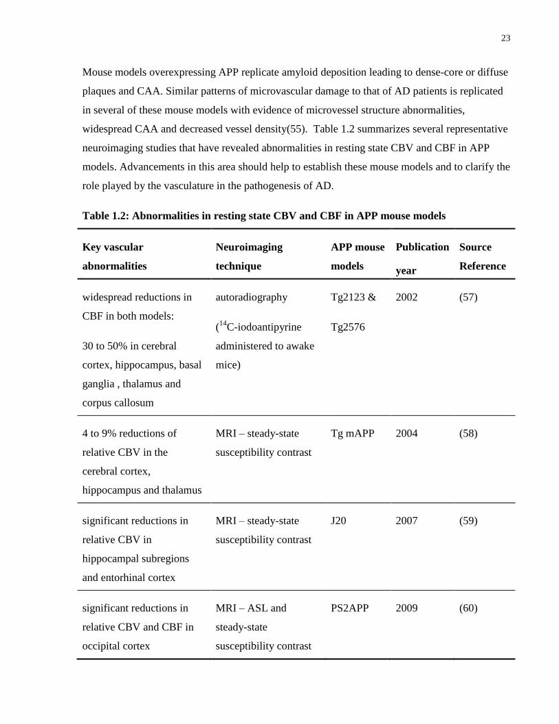
Mouse models overexpressing APP replicate amyloid deposition leading to dense-core or diffuse
plaques and CAA. Similar patterns of microvascular damage to that of AD patients is replicated
in several of these mouse models with evidence of microvessel structure abnormalities,
widespread CAA and decreased vessel density(55). Table 1.2 summarizes several representative
neuroimaging studies that have revealed abnormalities in resting state CBV and CBF in APP
models. Advancements in this area should help to establish these mouse models and to clarify the
role played by the vasculature in the pathogenesis of AD.
Table 1.2: Abnormalities in resting state CBV and CBF in APP mouse models
Key vascular
abnormalities
Neuroimaging
technique
APP mouse
models
Publication
year
Source
Reference
widespread reductions in
CBF in both models:
30 to 50% in cerebral
cortex, hippocampus, basal
ganglia , thalamus and
corpus callosum
autoradiography
(14
C-iodoantipyrine
administered to awake
mice)
Tg2123 &
Tg2576
2002 (57)
4 to 9% reductions of
relative CBV in the
cerebral cortex,
hippocampus and thalamus
MRI – steady-state
susceptibility contrast
Tg mAPP 2004 (58)
significant reductions in
relative CBV in
hippocampal subregions
and entorhinal cortex
MRI – steady-state
susceptibility contrast
J20 2007 (59)
significant reductions in
relative CBV and CBF in
occipital cortex
MRI – ASL and
steady-state
susceptibility contrast
PS2APP 2009 (60)

24
1.7 Structure and organization of this thesis
The body of this thesis comprises three manuscripts; Chapters 2 and 4 are reproduced from the
original peer-reviewed publication with only minor edits.
Chapter 2 describes the development of a technique to measure CBV in the mouse brain using
micro-CT. Key features of the described method are vascular perfusion under controlled
pressure, registration of the micro-CT images to an MRI anatomical brain atlas and re-scaling of
micro-CT intensities to CBV units with selectable exclusion of major vessels. As an application
of the methodology, two hypotheses are tested, namely, 1- CBV differs over anatomical brain
regions in the mouse; and 2- high energy demanding primary sensory regions of the cortex have
locally elevated CBV.
Chapter 3 describes a study in the TgCRND8 model of AD in which regional patterns of brain
volume and small-vessel cerebral blood volume (sv-CBV) are measured with MRI and micro-
CT, respectively. These metrics are compared with amyloid plaque load as detected by
immunohistochemistry.
Chapter 4 describes robust mapping of CBF over 3D brain regions using am-CASL. To provide
physiological data for CBF modeling, the carotid artery blood velocity distribution is
characterized using pulsed-wave Doppler ultrasound. These blood velocity measurements are
utilized in simulations that optimize inversion efficiency for parameters meeting MRI gradient
duty cycle constraints. A rapid slice positioning algorithm is developed and evaluated to provide
accurate positioning of the labeling plane. To account for enhancement of T1 due to
magnetization transfer, a binary spin bath model of MT is utilized to provide a more accurate
estimate of CBF. Finally, a study of CBF is conducted on ten mice providing values of inversion
efficiency and regional variation in CBF over 12 brain regions.
Chapter 5 provides a summary of the results of this thesis and a discussion of further technical
considerations for the perfusion-related metrics developed and tested. The material covered in
this chapter extends the discussion beyond that in the body of this thesis and considers future
directions.
25
Chapter 2 Measurement of Cerebral Blood Volume in Mouse Brain Regions
using Micro-computed Tomography
2.1 Foreword
The work in this chapter was previously published as:
Chugh BP, Lerch JP, Yu LX, Pienkowski M, Harrison RV, Henkelman RM, Sled JG.
Measurement of cerebral blood volume in mouse brain regions using micro-computed
tomography. Neuroimage 2009 Oct;47(4):1312-1318.
2.2 Introduction
Micro-computed tomography (micro-CT) can provide detailed 3D images of the mouse vascular
architecture(61). Recent applications of micro-CT to the mouse cerebral circulation include the
systematic classification of major vessels(62), the detection of atherosclerotic lesions around the
circle of Willis(63), and the co-registration of capillary-level views of the circulation with the
macroscopic vasculature(64). The use of this technique in the mouse is motivated by a desire to
better understand mouse models of human diseases.
This study describes the application of micro-CT to measure cerebral blood volume (CBV) for
characterizing total vascularity in 3D regions of the mouse brain. CBV is defined as the total
volume of blood in a given unit volume of brain(5). Measurement of CBV in local regions of the
mouse brain is of particular interest for delineating the phenotypes of models of
neurodegenerative diseases that alter cerebral vasculature, such as Alzheimer's disease(48).
Before the advent of suitable 3D imaging technologies, the CBV of the whole mouse brain was
measured by detecting intravascular radionuclides(36). More recently, regional values of CBV
were obtained using magnetic resonance imaging (MRI)(38); however, resolution was limited to
0.1 mm × 0.1 mm × 0.6 mm due to the time constraints of in vivo MRI scanning. Another

26
technique that allows a higher resolution for CBV mapping is multi-photon laser scanning
microscopy(37); however, available optics and depth of light penetration limit this technique to
the superficial 0.6 mm of cortex over small fields of view. Micro-CT measurement of CBV
provides both high-resolution and whole brain coverage for characterizing 3D regions.
In this study, we present a methodology by which CBV can be measured as the percentage of a
volume of tissue occupied by a perfused radio-opaque silicon rubber that remains intravascular.
We utilize the principle that for a voxel filled with two components, tissue and radio-opaque
contrast agent, the micro-CT image intensity is a weighted average of the attenuation coefficients
of each component(65). Thus, the micro-CT image intensity is linearly related to the proportion
of a voxel's volume that is occupied by radio-opaque contrast agent.
The procedure outlined in this study involves several innovative refinements to standard micro-
CT specimen preparation and analysis. First, to permit reproducible measurement of CBV, radio-
opaque vascular casts were prepared under controlled pressure. Second, to permit regional
comparisons, micro-CT images were registered to an MRI anatomical brain atlas. Third, to better
reflect the contribution of local microvessels to CBV, major vessels were excluded from the
analysis.
We also address the hypotheses that differences in CBV exist over anatomical brain regions and
that highly active primary sensory cortical areas have a particularly rich vascularization to meet
their high metabolic demands(66; 67). Specifically, we examine the possibility that primary
sensory cortex has a relatively high CBV in the non-stimulated condition, reflecting more dense
patterns of vascularization.
2.3 Materials and Methods
The steps to measure CBV in regions of the mouse brain were: (i)- the cerebral vasculature was
filled with Microfil (Flow Tech, Inc., Carver, MA, USA), a radio-opaque silicone rubber
containing particulate lead chromate and lead sulfate and known for minimal shrinkage(41); (ii)-
micro-CT images were acquired; (iii)- micro-CT images were re-scaled to CBV units; (iv)- CBV
images were co- registered to an MRI anatomical brain atlas; (v)- CBV was measured over brain
27
regions; (vi)- small vessel CBV (sv-CBV) was calculated by major vessel masking; (vii)-
regional CBV values were analyzed. Each step is detailed in the following sections.
2.3.1 Filling the cerebral vasculature with Microfil
Nine female C57BL/6 mice (Charles River Laboratories, Wilmington, MA, USA), weighing 17–
25 g, were anesthetized with an intraperitoneal injection (IP) of 100 μg ketamine per gram of
body weight (Pfizer, Kirkland, QC, Canada), 20 μg of xylazine per gram of body weight (Bayer
Inc., Toronto, Canada) and 3 μg of the vasodilator, acepromazine maleate(68), per gram of body
weight (Vetoquinol, Lavaltrie, QC, Canada), then given an IP injection of heparin (200 U)
(Organon Canada Ltd., Toronto, Canada). The inferior vena cava and descending aorta were
ligated. A 24-gauge IV catheter (Becton Dickinson Infusion Therapy System Inc., UT, USA)
was inserted into the left ventricle, sealed in place using the adhesive Loctite 404 (McMaster-
Carr, GA, USA) and connected to a pressure- controlled pump (Model PS/200, Living Systems
Instrumentation, VT, USA). All incidental cuts were sealed. A slit in the right atrium provided
outflow.
To minimize variation in CBV due to vessel inflation, the pressure at which Microfil
polymerizes should be uniform. Warm heparinized (5 U/mL) phosphate buffered saline (Wisent
Inc., St-Bruno, QC, Canada) was perfused at 50 mm Hg for 5 min at a filling rate of 2 mL/min,
followed by Microfil at room temperature at 150 mm Hg for 10 min at a filling rate of 0.25
mL/min. The filling rate was determined based on the rate of volume change in a graduated
cylinder containing the infusate. The pump was stopped, the slit in the right atrium sealed and the
pump restarted at 30 mm Hg, approximating normal capillary pressure(69; 70). At this uniform
pressure, the Microfil polymerized over 90 min at room temperature. Microfil has previously
been shown to remain intravascular(40); we quantified the completeness of the perfusions in a
section that follows.
2.3.2 Acquiring micro-CT images
In preparation for micro-CT scans, dissected skulls (devoid of external soft tissue and lower jaw)
were fixed for 12 h at 4 ± 1 °C in 10% buffered formalin phosphate (Fisher Scientific Company,
Ottawa, Canada). To avoid partial volume and beam hardening artifacts, the skulls were
decalcified in 5% formic acid (Fisher Scientific Company, Ottawa, Canada) at 50 °C for 24 h and
28
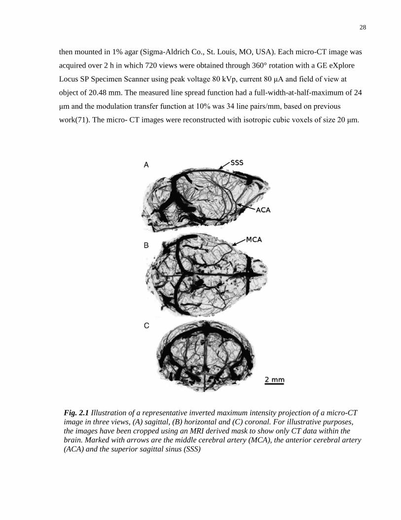
then mounted in 1% agar (Sigma-Aldrich Co., St. Louis, MO, USA). Each micro-CT image was
acquired over 2 h in which 720 views were obtained through 360° rotation with a GE eXplore
Locus SP Specimen Scanner using peak voltage 80 kVp, current 80 μA and field of view at
object of 20.48 mm. The measured line spread function had a full-width-at-half-maximum of 24
μm and the modulation transfer function at 10% was 34 line pairs/mm, based on previous
work(71). The micro- CT images were reconstructed with isotropic cubic voxels of size 20 μm.
Fig. 2.1 Illustration of a representative inverted maximum intensity projection of a micro-CT
image in three views, (A) sagittal, (B) horizontal and (C) coronal. For illustrative purposes,
the images have been cropped using an MRI derived mask to show only CT data within the
brain. Marked with arrows are the middle cerebral artery (MCA), the anterior cerebral artery
(ACA) and the superior sagittal sinus (SSS)

29
2.3.3 Measuring completeness of the perfusion
A potential source of error is incomplete perfusion of the brain with Microfil, leading to
underestimated CBV. Thus, the proportion of vessels filled with Microfil was measured.
Specifically, five of the perfused specimens were paraffin embedded and sixteen 5 μm coronal
sections were cut: four samples (spaced 10 μm apart) were cut at four locations (defined by
frontal cortex, striatum, hippocampus and superior colliculus). To calculate the percentage of
vessels filled with Microfil, we stained the sections with hematoxylin and under 20×
magnification, scored vessels in randomly selected fields according to whether Microfil was seen
in the lumen. The data were categorized by specimen (out of 5) and brain location (out of 4). To
test whether the completeness of Microfil perfusion significantly differed between the locations
examined, an analysis of variance (ANOVA) was performed on a linear mixed effect model of
the data, with one fixed effect (location) and one random effect (specimen) using the statistical
program R, available at http://www.r-project.org/.
2.3.4 Re-scaling the micro-CT images to CBV units
The CBV of each tissue voxel is the ratio of the concentration of Microfil in that tissue voxel to
the concentration of Microfil in the vasculature. This was computed for each micro-CT image,
by using simple volume averaging of the components of the voxel, which were assumed to be
Microfil and tissue. The tissue's radio-opacity is similar to 1% agar and is much lower than that
of Microfil.
To study the relative radio-opacities of the components of each voxel, an additional C57BL/6
mouse was perfused just with phosphate buffered saline (PBS), without Microfil, prior to
scanning. This specimen was imaged in 1% agar together with an external slab of Microfil and
the average radio- opacity in all components was compared. We also tested uniformity in the CT
intensity through the depth of the image, by measuring the percentage variation in the line profile
through the tissue.
Each micro-CT image was re-scaled into CBV units by the following equation:
)/()%(100 AGARMICROFILAGARORIGINALCBV IIIII , [2.1]
30
where IORIGINAL denotes the x-ray attenuation coefficient of the tissue voxels, IAGAR denotes the
average x-ray attenuation coefficient of voxels in the 1% agar and IMICROFIL denotes the average
x-ray attenuation coefficient of voxels completely filled with Microfil. Below, the terms “image
intensity” and “x-ray attenuation coefficient” are used interchangeably since the CT images were
processed in arbitrary units.
The background intensity, IAGAR, was computed as the average intensity of approximately 10,000
voxels in the 1% agar. We applied a custom written program to automatically trace vessel
centerlines and determine vessel diameters. This automated vessel tracking program traces the
centerlines of tubular objects by maintaining equal distance from the lumen wall as determined
by the image intensity gradient along rays perpendicular to the vessel centerline(72). To
normalize the intensity of each individual image, IMICROFIL was computed as the average intensity
of approximately 20,000 voxels at centerline positions of vessel segments with diameter between
0.1 and 0.2 mm. Use of these vessel segments ensured that the voxels were completely filled
with Microfil.
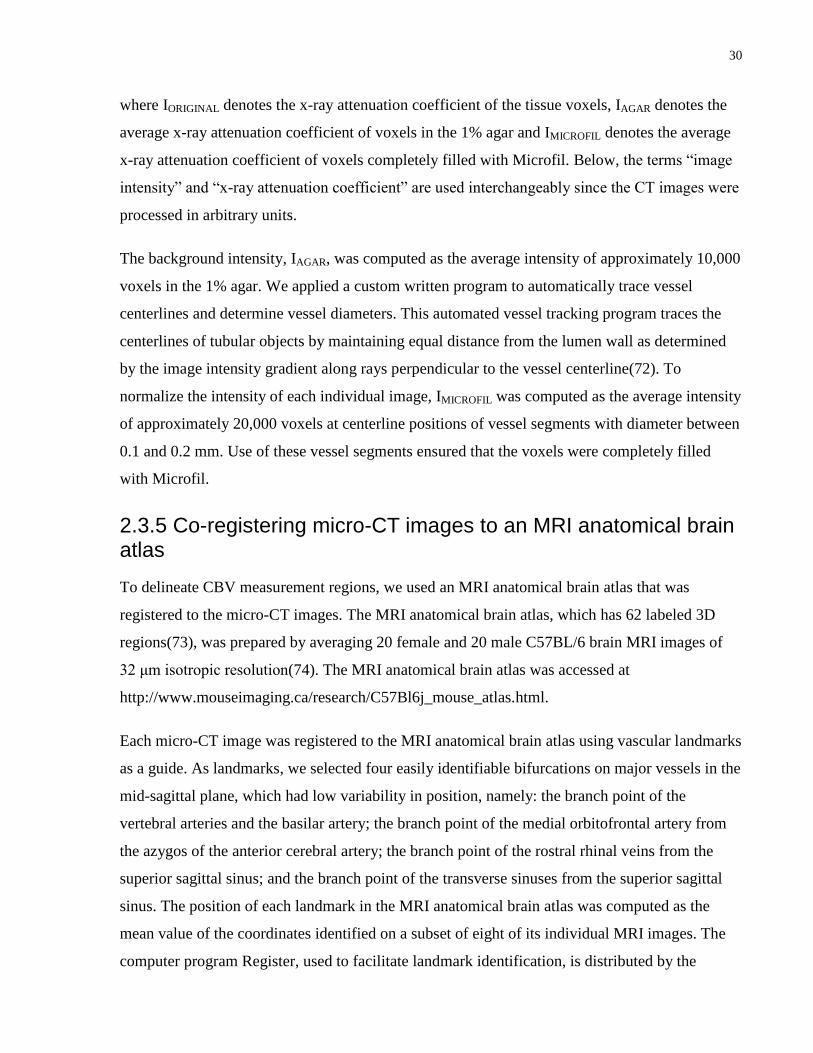
2.3.5 Co-registering micro-CT images to an MRI anatomical brain atlas
To delineate CBV measurement regions, we used an MRI anatomical brain atlas that was
registered to the micro-CT images. The MRI anatomical brain atlas, which has 62 labeled 3D
regions(73), was prepared by averaging 20 female and 20 male C57BL/6 brain MRI images of
32 μm isotropic resolution(74). The MRI anatomical brain atlas was accessed at
http://www.mouseimaging.ca/research/C57Bl6j_mouse_atlas.html.
Each micro-CT image was registered to the MRI anatomical brain atlas using vascular landmarks
as a guide. As landmarks, we selected four easily identifiable bifurcations on major vessels in the
mid-sagittal plane, which had low variability in position, namely: the branch point of the
vertebral arteries and the basilar artery; the branch point of the medial orbitofrontal artery from
the azygos of the anterior cerebral artery; the branch point of the rostral rhinal veins from the
superior sagittal sinus; and the branch point of the transverse sinuses from the superior sagittal
sinus. The position of each landmark in the MRI anatomical brain atlas was computed as the
mean value of the coordinates identified on a subset of eight of its individual MRI images. The
computer program Register, used to facilitate landmark identification, is distributed by the
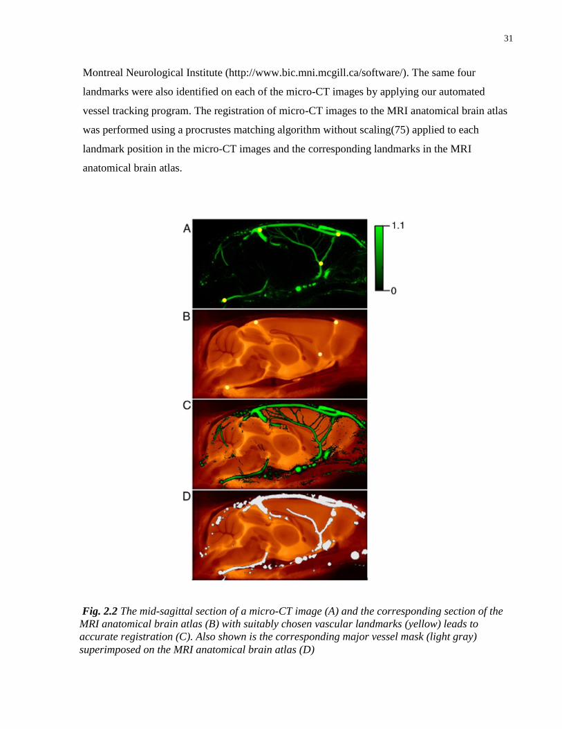
31
Montreal Neurological Institute (http://www.bic.mni.mcgill.ca/software/). The same four
landmarks were also identified on each of the micro-CT images by applying our automated
vessel tracking program. The registration of micro-CT images to the MRI anatomical brain atlas
was performed using a procrustes matching algorithm without scaling(75) applied to each
landmark position in the micro-CT images and the corresponding landmarks in the MRI
anatomical brain atlas.
Fig. 2.2 The mid-sagittal section of a micro-CT image (A) and the corresponding section of the
MRI anatomical brain atlas (B) with suitably chosen vascular landmarks (yellow) leads to
accurate registration (C). Also shown is the corresponding major vessel mask (light gray)
superimposed on the MRI anatomical brain atlas (D)

32
2.3.6 Measuring CBV over brain regions
Our goal was to reduce variability in CBV caused by registration error. Of the 62 regions in the
MRI anatomical brain atlas, we selected all 13 regions that were larger than 5 mm3. Selection of
this threshold was based on a registration simulation that relied on the measured variability in the
position of the vascular landmarks. This simulation involved generating five transformed copies
of a given micro-CT image by adding random offsets derived from observed positional variation
in vascular landmarks; for the transformed images the coefficient of variation (COV) was
calculated region by region and an arbitrary cutoff at 10% COV led us to retain regions larger
than 5 mm3.
Misregistration error can significantly bias CBV when there is a great difference between the
values of neighboring regions. To reduce this bias, we incrementally eroded the boundary of
each region on the MRI anatomical brain atlas using a six neighbor binary morphological
operator(76). We selected 0.15 mm as the depth of erosion because the CBV values of gray
matter regions that border white matter regions stabilized after this amount of erosion.
The following computational method was applied to obtain CBV values. The average CBV and
standard error were calculated for each of the selected 13 brain regions. To map CBV over the
cerebral cortex, we solved Laplace's equation to generate field-lines from the inner to the outer
cortical surface. This method has previously been applied to map human cortical thickness(77)
and has recently been adapted to determine cortical thickness in the mouse brain(78). Next, CBV
was averaged along each field-line and the value was projected to the mid-cortical surface; this
was done through the entire thickness of the cortex, without eroding the boundary. To determine
CBV through the depth of the cortex, the field-lines were divided into ten equal parts, which
collectively defined ten layers.
2.3.7 Determining sv-CBV by major vessel masking
To emphasize the contribution of local microvessels to CBV, major vessels were excluded using
a selectable diameter threshold that was arbitrarily chosen to be 100 μm. We formed a major
vessel mask by our automated vessel tracking program to identify vessels in the micro-CT
images greater than 100 μm in diameter. The metric, small-vessel CBV (sv-CBV), was defined
as the total volume of blood, for vessels with diameter under 100 µm, as a percentage of the
33
region’s volume and was calculated analogously to CBV after deletion of data from the micro-
CT images that was associated with the major vessel mask; sv-CBV was measured over the 13
brain regions and the cerebral cortex.
Fig. 2.3 CBV maps over the surface of the cerebral cortex, averaged over nine mice: (A-C)
show total CBV maps for the dorsal, right lateral and left lateral surfaces, respectively; (D-F)
show the sv-CBV maps; (G and H) show the right and left surfaces marked with manually
delineated visual, auditory and somatosensory areas (in blue, yellow, and red respectively).
For each sensory modality a core region (dark shading) is indicated, which includes visual
areas V1 and V2 and auditory areas A1 and A2. The large somatosensory area (pink) denotes
primary somatosensory areas including the extensive barrel cortex region.
34
2.3.8 Analyzing regional CBV values
Using R, a statistical analysis was performed on the CBV data, which were categorized by
specimen (N = 9), brain region (N = 13 and the type of metric (total CBV or sv-CBV). An
ANOVA was performed on a linear mixed effect model of the data, which had two fixed effects
(brain region and type of metric) and one random effect (specimen). The percentage difference
between total CBV and sv-CBV was also determined for each micro-CT image. To determine if
sv-CBV significantly differed between brain hemi-spheres, ten of thirteen regions were
segmented into portions in each hemisphere and the mean sv-CBV was graphically compared.
An ANOVA was performed with R, using a mixed effect linear model where hemisphere was the
fixed factor and specimen was the random factor.
To compare sv-CBV over regions of the cortex, the primary sensory areas were delineated on
right and left cortical maps based on published maps for the C57BL/6 mouse, prepared by
staining cytochrome oxidase(79), cytochrome oxidase and myelin(80) and
acetylcholinesterase(81).
All described animal procedures were approved by the Hospital for Sick Children Animal Care
Committee, subject to the Canadian Council on Animal Care.
2.4 Results
A representative example of one of the Micro-CT images is shown in three maximum intensity
projection views in Fig.2.1. All major arteries branching from the circle of Willis and major
returning veins and sinuses were identifiable, such as the middle cerebral artery (MCA), the
anterior cerebral artery (ACA) and the superior sagittal sinus (SSS) (marked with arrows in
Fig.2.1). Inspection of the images provided no evidence that Microfil had leaked outside of
vessels.
Histological analysis revealed that over the group of mice the average ± standard error of mean
(SEM) percentage of vessels filled with Microfil was 93 ± 3%, which may have been an
underestimate due to minor displacement of Microfil fragments during slide preparation. The
35
completeness of Microfil perfusion did not significantly differ between the locations examined
(F = 0.72, p = 0.5).
The average radio-opacities of Microfil and 1% agar were 3700 ± 100 Hounsfield units and 0 ±
100 Hounsfield units, respectively. In support of the assumption that CT intensity varies
negligibly through the depth of images, we found that the line profile through the unperfused
brain tissue, described in section 2.3.4, had a maximum variation of 5 Hounsfield units.
A representative example of vascular-landmark registration of a micro-CT image to the
anatomical brain atlas is shown in Fig.2.2 (A,B,C). The mean value (N = 9) for the standard
deviation of the registered coordinates of the four vascular landmarks was 0.15 mm. A
representative example of the overlay of a major vessel mask on the MRI anatomical brain atlas
is shown in Fig.2.2 (D). In regions where multiple vessels converged, the diameters of the
vessels tended to be overestimated by our automated vessel tracking program.
Cortical maps of total CBV, averaged across nine mice, are shown in Fig.2.3 (A,B,C) and maps
of sv-CBV in Fig.2.3 (D,E,F). The posterior cortex had an elevated sv-CBV compared to the
average cortical sv-CBV of 4.6±0.4. The primary sensory areas that are delineated(79–81) in
Fig.2.3 (G,H) indicate a higher value of CBV in the primary visual and auditory areas relative to
the average value of the cortex. However, there does not appear to be a higher than average value
of the CBV in the primary somatosensory areas.
Table 2.1 summarizes CBV data sets for both total and sv-CBV. To illustrate the shapes, relative
sizes and locations of the 13 brain regions, three sagittal slices have been labeled with each
region in Fig.2.4.
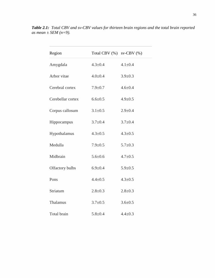
36
Table 2.1: Total CBV and sv-CBV values for thirteen brain regions and the total brain reported
as mean ± SEM (n=9).
Region Total CBV (%) sv-CBV (%)
Amygdala 4.3±0.4 4.1±0.4
Arbor vitae 4.0±0.4 3.9±0.3
Cerebral cortex 7.9±0.7 4.6±0.4
Cerebellar cortex 6.6±0.5 4.9±0.5
Corpus callosum 3.1±0.5 2.9±0.4
Hippocampus 3.7±0.4 3.7±0.4
Hypothalamus 4.3±0.5 4.3±0.5
Medulla 7.9±0.5 5.7±0.3
Midbrain 5.6±0.6 4.7±0.5
Olfactory bulbs 6.9±0.4 5.9±0.5
Pons 4.4±0.5 4.3±0.5
Striatum 2.8±0.3 2.8±0.3
Thalamus 3.7±0.5 3.6±0.5
Total brain 5.8±0.4 4.4±0.3
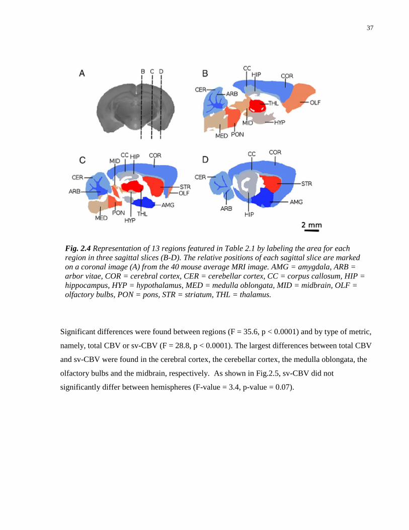
37
Significant differences were found between regions (F = 35.6, p < 0.0001) and by type of metric,
namely, total CBV or sv-CBV (F = 28.8, p < 0.0001). The largest differences between total CBV
and sv-CBV were found in the cerebral cortex, the cerebellar cortex, the medulla oblongata, the
olfactory bulbs and the midbrain, respectively. As shown in Fig.2.5, sv-CBV did not
significantly differ between hemispheres (F-value = 3.4, p-value = 0.07).
Fig. 2.4 Representation of 13 regions featured in Table 2.1 by labeling the area for each
region in three sagittal slices (B-D). The relative positions of each sagittal slice are marked
on a coronal image (A) from the 40 mouse average MRI image. AMG = amygdala, ARB =
arbor vitae, COR = cerebral cortex, CER = cerebellar cortex, CC = corpus callosum, HIP =
hippocampus, HYP = hypothalamus, MED = medulla oblongata, MID = midbrain, OLF =
olfactory bulbs, PON = pons, STR = striatum, THL = thalamus.
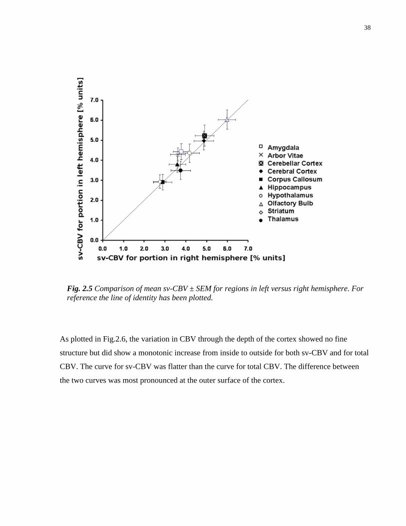
38
As plotted in Fig.2.6, the variation in CBV through the depth of the cortex showed no fine
structure but did show a monotonic increase from inside to outside for both sv-CBV and for total
CBV. The curve for sv-CBV was flatter than the curve for total CBV. The difference between
the two curves was most pronounced at the outer surface of the cortex.
Fig. 2.5 Comparison of mean sv-CBV ± SEM for regions in left versus right hemisphere. For
reference the line of identity has been plotted.
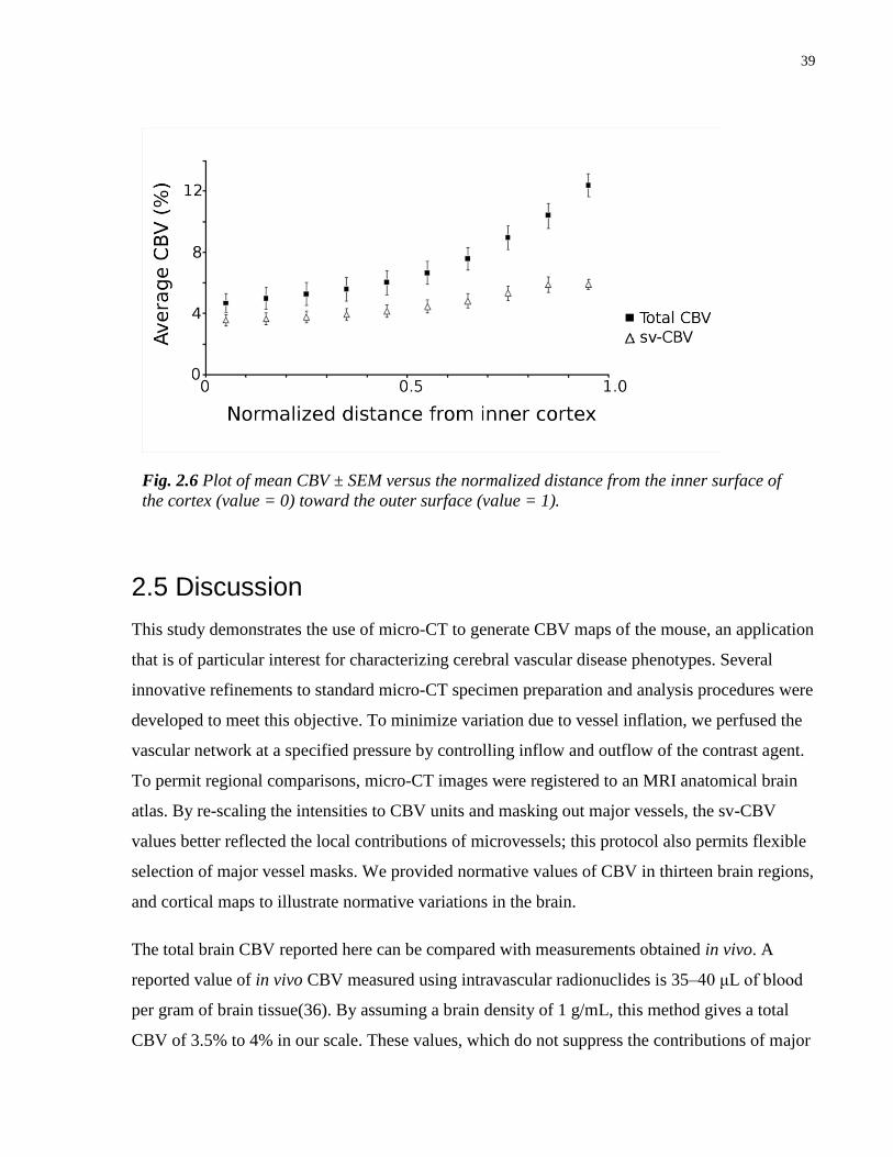
39
2.5 Discussion
This study demonstrates the use of micro-CT to generate CBV maps of the mouse, an application
that is of particular interest for characterizing cerebral vascular disease phenotypes. Several
innovative refinements to standard micro-CT specimen preparation and analysis procedures were
developed to meet this objective. To minimize variation due to vessel inflation, we perfused the
vascular network at a specified pressure by controlling inflow and outflow of the contrast agent.
To permit regional comparisons, micro-CT images were registered to an MRI anatomical brain
atlas. By re-scaling the intensities to CBV units and masking out major vessels, the sv-CBV
values better reflected the local contributions of microvessels; this protocol also permits flexible
selection of major vessel masks. We provided normative values of CBV in thirteen brain regions,
and cortical maps to illustrate normative variations in the brain.
The total brain CBV reported here can be compared with measurements obtained in vivo. A
reported value of in vivo CBV measured using intravascular radionuclides is 35–40 μL of blood
per gram of brain tissue(36). By assuming a brain density of 1 g/mL, this method gives a total
CBV of 3.5% to 4% in our scale. These values, which do not suppress the contributions of major
Fig. 2.6 Plot of mean CBV ± SEM versus the normalized distance from the inner surface of
the cortex (value = 0) toward the outer surface (value = 1).

40
vessels, are in reasonable agreement with our sv-CBV measurement of 4.4 ± 0.3%, but lower
than the total CBV of 5.8 ± 0.4%. A possible explanation for this difference is that by preparing
the radio-opaque vascular casts at a pressure of 30 mm Hg, the venous vessels, which contain
most of the blood in the brain, were distended past their normal physiological point. Most of this
effect would have been accounted for by masking of the major sinuses and veins. However, the
remaining slight difference is likely owing to the large amount of blood in the venules, which
may also be distended in the pressure control setup. Nevertheless, the CBV values measured in
this study are in reasonable agreement with the in vivo CBV values, as obtained using
intravascular radionuclides.
To obtain reproducible values of CBV, we stress that the radio-opaque vascular casts must be
prepared at a well-defined pressure. As the main contribution to the CBV comes from highly
compliant venules and veins, failure to control this factor would likely lead to a large variation in
results. We set the pressure close to an assumed average capillary pressure of about 30 mm Hg,
which has not been directly measured in the mouse brain, but which provides a commonly
accepted estimate for capillaries in the systemic circulation(69; 70). In this case, we can expect
the sv-CBV values to be similar to the in vivo value. The close correspondence of sv-CBV
between bilaterally symmetric regions (see Fig.2.5) supports the notion that the image
registration was accurate. Another factor affecting reproducibility is the completeness of major
vessel masking. The purpose of applying our automated vessel tracking program was to ensure
greater accuracy of the major vessel masking. Since vessels with diameter greater than 100 μm
represent approximately 1% of total brain volume, moderate overestimate of the mask can be
expected to have a negligible effect on sv-CBV. Masking of finer vessels in the brain could also
be performed, in future, with micro-CT scanners of higher resolution and signal-to-noise ratio.
As brain atlases become more refined, one likely interest will be to measure sv-CBV in
increasingly fine regions. In such cases, registration will pose a fundamental limitation on the
size of the region over which sv-CBV can be accurately mapped. The registration method used in
this study was based on vascular landmarks that have 0.15 mm root mean squared variability in
position. In Fig.2.3, a comparison is made between total CBV and sv-CBV. By masking the
major vessels, the sv-CBV was shown to be more spatially uniform over structurally similar
regions of the cortex. The ability to mask vessels also poses a limitation on the size of the region
that can be studied. In small regions, a major vessel may constitute a large fraction of the
41
measurement volume; this artifact could outweigh microvascular variation and lead to false
interpretation. For example, a 100 μm vessel that passes through a measurement volume of 1
mm3 will increase an average CBV of 4% to about 5%, leading to a 25% overestimate. Since the
masking is a function of resolution and SNR, improvements in micro-CT image quality will
translate to greater control of the size of the region that can be mapped.
One of our scientific questions was whether primary sensory areas of cortex have a higher local
sv-CBV compared to other cortical regions. This question was based on the hypothesis that
sensory input areas such as visual, auditory and somatosensory cortices are highly active, with
metabolic demands that might be met with a privileged blood oxygen supply. It is well known
from hemodynamic based functional imaging techniques such as optical imaging of intrinsic
signals(46) that under sensory stimulation, there is a significant CBV change in primary cortex
compared to less active association cortex(45; 82). Although the changes described in these
studies are transient responses to stimulation, it is possible that primary sensory cortex has a
more permanent vascular specialization(66). Comparison of the cortical map of sv-CBV in
Fig.2.3 with maps showing locations of the major sensory cortical areas, suggests that sv-CBV is
elevated in both visual and auditory areas, though not convincingly in the primary somatosensory
area. This likely suggests that there is not a specialized blood supply for the entire somatosensory
area. One reason for this may be that the hypothesized increased blood oxygen supply to highly
active brain areas may be most readily detectable at the capillary network level(66) whereas this
definition of sv-CBV includes feeding arterioles and drainage venules that contain a significant
proportion of the blood.
The sv-CBV increased from the inner to the outer boundary of the cerebral cortex, which was
consistent with the depth variation of cortical microvessel density observed with confocal
microscopy in rats for vessels with diameter under 50 μm(83) and in humans both with and
without major vessel masking above 10 μm in diameter(84). Unlike those studies of microvessel
density, however, the sv-CBV, plotted in Fig.2.6, did not sharply decline at the outer boundary,
but appeared to level off toward the outer 20% of the depth. This pattern of variation supports a
model of vascular organization where capillary-rich beds and their associated feeding arterioles
and drainage venules are concentrated near the outer boundary of the cortex.

42
Mapping sv-CBV over an anatomical brain atlas could lead to better understanding of vascular
degeneration in dementia models, as well as the angiogenesis following treatments. Our method
of sv-CBV mapping improves on past work as it can be used to determine CBV phenotypes in
small 3D regions of the mouse brain. With continued development of better mouse brain atlases
and genetic models, we anticipate that this method to measure sv-CBV will lead to a better
characterization of vascularity in mouse models of cerebral vascular disease.
43
Chapter 3 High Resolution MRI and Micro-CT Imaging show Microvascular and Neuroanatomical Changes in a Mouse Model of Alzheimer’s
Disease
3.1 Foreword
At the time of completion of this thesis, the work in this chapter was not published in a peer-
reviewed journal.
3.2 Introduction
Research on Alzheimer’s Disease (AD) etiology has been dominated by the amyloid cascade
hypothesis, which holds that deposition of extracellular Aβ in the brain is causative in the
biochemical progression to AD(85). In this hypothesis, an imbalance between Aβ production and
clearance initiates a multi-step cascade leading to the histopathological hallmarks of AD
including neurodegeneration and synaptic failure with associated failure of neurotransmitter
pathways. A major line of support for the amyloid cascade hypothesis is that transgenic mice,
expressing a mutant form of the human amyloid precursor protein (APP) gene, develop amyloid
plaque burden and cognitive symptoms such as spatial learning deficits(86). One of the major
challenges to this hypothesis has been that the breakdown of vulnerable neuronal systems,
especially those involved in memory, have often appeared to be disassociated from amyloid
deposition, while it has been argued that the clinical impairments are better explained by the
regional pattern of neurofibrillary tangles(87). The amyloid cascade hypothesis has been
supported, however, by controlled studies on APP mouse models that first develop diffuse and
then fibrillar Aβ plaques, which appear to precede any neurological damage. In fact, Aβ42
immunization in an APP model known as TgCRND8 has been shown to reverse behavioural and
cognitive abnormalities and is coincident with approximately half as many dense-core
plaques(88).

44
Several studies support the notion that microvascular changes, which include decreases in
vascular density, atrophic and coiling vessels, and glomerular loop formations, are associated
with the progression of AD(48; 89). There is a known association between amyloid plaques and
damage to the architecture of blood vessels in mouse models of AD(90). Microvascular
abnormalities may not directly result in perfusion changes, but may hinder the clearance of
amyloid plaques(56). Although there are several mechanisms for clearing Aβ, including
degradation of amyloid by microglia or by proteases and drainage of amyloid via the periarterial
interstitial fluid, it has been found that direct transport of Aβ across the blood-brain-barrier
(BBB) is normally one of the most efficient(91; 92). This direct vascular clearance route can
become compromised due to BBB damage or when the BBB is overwhelmed by excessive
production of Aβ. Despite the growing evidence for vascular involvement in AD, however,
limited work has been done to characterize regional changes in microvasculature.
Regional changes in the microvasculature can be characterized by 3D imaging techniques that
measure cerebral blood volume (CBV). This has been developed in mice using magnetic
resonance imaging (MRI) and at higher resolutions with micro-computed tomography (micro-
CT), a technique that can produce detailed 3D images of the cerebral vasculature(93). In vivo
measurement of CBV, using MRI in transgenic AD-afflicted mice, has revealed altered CBV in
the cerebral cortex, the hippocampus and the thalamus(58). Changes in brain morphology that
are characteristic of AD have also been observed in different transgenic mouse models of
AD(94; 95). Relative to histological methods, these neuroimaging approaches provide a
macroscopic view of regional variation, which can often be a prelude to more detailed
investigations.
A promising model of AD is the double APP695 mutant, with Swedish and Indiana mutations,
known as TgCRND8 that expresses a high ratio of Aβ42 to Aβ40 and presents with an
aggressive amyloid pathology(96). These mice have low survival rates and their dense-core
plaques, widespread by 16-35 weeks, have been associated with dystrophic neurites(97; 98),
synaptic degeneration and inflammatory response with activated microglia and astrocytes
appearing concurrently with plaques(99). As with other APP mouse models(100), TgCRND8
mice do not show the extent of neuronal loss observed in human AD(99), although selective loss
has been reported for cholinergic neurons in the vicinity of plaques at seven month of age(101)
and for neurons in the hippocampus at five months of age(102), a major site for plaque
45
accumulation in TgCRND8 mice(99). This neuronal degeneration may be associated with brain
atrophy, though swelling occurs in 28% of axons in the vicinity of plaques of five month old
TgCRND8 mice(98) and infiltration of enlarged microglial cells and hypertrophic astrocytes
accompanies amyloid deposition(101); both of these latter factors may contribute to brain
hypertrophy. Vascular abnormalities in the TgCRND8 model include blood brain barrier damage
with increased tortuosity, reduced number of microvascular branches(103) and widespread
cerebral amyloid angiopathy(104). Decreased microvessel density in the cerebral cortex of six
month old TgCRND8 mice was observed on 2D immunofluorescent images labeled for platelet
endothelial cell adhesion molecule-1(PECAM-1) (103). Despite the abundance of microscopic
evidence for vascular and morphological changes in the TgCRND8 brain, to date, no study has
provided a macroscopic view of these changes over the entire brain.
The present study characterizes and compares, in five month old TgCRND8 mice, the following
three metrics: (i)- regional brain volume measured by MRI; (ii)- small-vessel CBV (sv-CBV),
measured by micro-CT, where sv-CBV is like CBV in that it measures the percentage of a
region’s volume occupied by blood vessels, however, only for small-vessels with diameter less
than 100 μm; and, (iii)- plaque load, measured by immunohistochemistry. Plaque load is the
percentage of each region’s area seen on histological sections that is covered by amyloid
plaques. These three metrics were evaluated over anatomical regions of the brain delineated with
high-resolution MRI. Brain volume and sv-CBV were measured over 23 brain regions and
plaque load assessed in 15 regions.
3.3 Materials and Methods
3.3.1 Animals
The TgCRND8 colony was maintained in a 129SvEv background and heterozygote experimental
animals were derived from crosses of TgCRND8 males with C57BL/6 females. PCR-based
genotyping was performed both at the age of weaning and at sacrifice, namely, 3 weeks and
23±2 weeks. A total of 20 TgCRND8 mice (16 males and 4 females) and 27 controls (13 males
and 14 females), underwent the following procedures, approved by the Hospital for Sick
Children Animal Care Committee, subject to the Canadian Council for Animal Care.
46
3.3.2 Specimen Preparation
The cerebral vasculature of each mouse was perfused under controlled pressure with a radio-
opaque silicone rubber, Microfil (Flow Tech, Inc., Carver, MA, USA), using the previously
described protocol(93). To prepare for MR imaging, the dissected skulls were sequentially
soaked in the following solutions: 12 hours in 4% paraformaldehyde (providing chemical
fixation), 5 days in phosphate buffered solution (PBS) and 0.01% sodium azide at 15°C and 7
days in 2 mM Prohance (Bracco Diagnostics Inc., Princeton, NJ) diluted in PBS at 15°C
(providing MRI contrast enhancement).
3.3.3 MR imaging
MR imaging was performed using a protocol customized for mouse applications(105).
Specimens were imaged using a 7.0-T MRI scanner (Varian Inc., Palo Alto, CA, USA) while
immersed in a proton-free susceptibility-matching fluid (Fluorinert FC-77, 3M Corp., St. Paul,
MN). The parameters used in the scans were optimized for grey/white matter contrast: T2 -
weighted, 3D fast spin-echo (ETL=6), with TR/TE= 2000/15 ms, NEX=2, field-of-view 25 x 14
x 14 mm and matrix size = 450 x 250 x 250, providing images with 56 µm isotropic voxels. The
total imaging time was 11 hours and 35 minutes.
3.3.4 Micro-CT imaging
To avoid partial volume and beam hardening artifacts in Micro-CT images, specimens were
decalcified by soaking for 2 days in 8% formic acid (Fisher Scientific Company, Ottawa, ON,
Canada) at 15°C following a two day soak in PBS. Micro-CT images were then acquired as
previously described(93).
3.3.5 Aβ Immunohistochemistry
Aβ was stained on 4 μm paraffin embedded coronal brain sections, four sections per brain (at
level of olfactory, striatum, hippocampus and cerebellum), with 4G8 anti-Aβ monoclonal
antibody (1:1000, Signet 9220-02), followed by overnight incubation at 4 ºC and development
using Avidin/Biotinylated enzyme Complex kit (Vector Labs, PK-6100) with visualization using
diaminobenzidine. Counterstaining was performed with hematoxalin and scanning was at 20X
(Hamamatsu Nanozoomer 2.0 RS scanner).
47
3.3.6 Computation of brain volume, sv-CBV and plaque load
All MR images were non-linearly registered to a neuroanatomical atlas with 62 segmented
regions, as previously described(73; 105). This procedure allowed each of the 62 regions defined
in the atlas to be outlined on the given MR image. Each micro-CT image underwent rigid-body
registration to the corresponding mouse brain’s MR image by manually selecting twenty
landmarks at vessel bifurcations in each image; the root-mean-square error of this registration,
expressed as mean±standard deviation for the group of 47 image pairs, was 12.5±4.8 µm. This
landmark registration was facilitated by contrast between the Microfil and surrounding tissue in
the MRI images. sv-CBV was computed by utilizing the principle that for a voxel filled with
two components, tissue and radio-opaque contrast agent, the micro-CT image intensity is a
weighted average of the attenuation coefficients of each component(93). To emphasize the
contribution of local microvessels to CBV, major vessels with diameter over 100 μm were
excluded using vessel tracking(72), as previously described(93).
Plaque load was calculated over each region of the brain using the following procedure: (i)-
regions of the images, described in section 3.3.5, were manually outlined with guidance from the
corresponding MRI image with a co-registered labeled regions mapped; (ii)- a bayesian
classifier(106) with non-informative prior was manually trained based on image pixel colour
with 900 training points, which included ambiguous cases, to distinguish pixels corresponding to
amyloid from those corresponding to Microfil and the remaining background using the computer
program Classify, distributed by the Montreal Neurological Institute. Fifteen regions were
manually outlined on the images of the histological slides and the percentage area classified as
amyloid plaque was computed for each region.
3.3.7 Statistical analysis
For each mouse brain, volume and sv-CBV were computed in the 23 largest anatomical regions
(see Table 3.1) of the brain atlas with the smallest region included being the dentate gyrus. To
test whether there was significant regional variation in brain volume, an ANOVA was performed
on a linear mixed effect model of the data, with two fixed effects (region and genotype) and one
random effect (specimen) using the statistical program R, available at http://www.r-project.org/.
Regional variation in sv-CBV was tested using the same procedure. Specific regional differences
were determined by conducting t-tests for individual regions and a false discovery rate, q ,was
48
computed corresponding to each p-value for the combined set of 23 volume measurements and
23 sv-CBV measurements based on the false discovery rate method(107). Percentage increases
in volume, illustrated in Fig. 3.1, were plotted after blurring the data with a kernel of 0.5 mm full
width at half maximum. To generate cortical surface plots shown in Fig. 3.2, sv-CBV was
averaged over field lines perpendicular to the cerebral cortex(77; 78), using the previously
described procedure(93).
To test for bilateral symmetry of regional brain volume, nineteen of the twenty three brain
regions were segmented into portions in each hemisphere and an ANOVA was performed using
a mixed effect linear model with region, genotype and hemisphere as fixed factors and specimen
as a random factor. An analogous ANOVA was applied to test for significant hemispheric
variation in sv-CBV.
An ANOVA was performed to test for variation of whole brain volume or average brain sv-CBV
with sex, in each case with a linear model with genotype and sex as fixed factors. An analogous
test for age related effects was also conducted.
To test for regional variation of plaque load, an ANOVA was performed on a linear mixed effect
model, with region as the fixed effect and specimen as the random effect. To test whether
percentage change in brain volume was significantly dependent on plaque load, an ANOVA was
performed on a linear mixed effect model of the data, with two fixed effects (region and plaque
load) and one random effect (specimen). Significant variation in sv-CBV with plaque load was
tested using an analogous ANOVA.
The sensitivity of the test for a relationship between sv-CBV and plaque load or percentage
change in brain volume and plaque load was estimated using power analysis. For each response
variable, statistical power was estimated based on a Monte Carlo simulation as a function of the
linear coefficient corresponding to plaque load. This coefficient in the linear-mixed effect model
with two fixed effects (region and plaque load) was systematically varied and ANOVA was
performed to test for significance (p-value < 0.05) with power estimated for 500 trials per
coefficient.
All computed parameters were expressed as mean ± standard-error-of-the-mean (SEM) unless
stated otherwise.
49
3.4 Results and Discussion
3.4.1 Global and local brain atrophy
TgCRND8 mice (n=20) had a total brain volume of 474±4 mm3 which was significantly
(p=0.0007) smaller than control mice (n=27) at 493±4 mm3. This is not a surprising finding as
global brain atrophy is prevalent in human AD patients(108) and has also been reported in some
APP mouse models(109). Based on a linear mixed effect model, regional brain volume varied
according to genotype (F1,45 = 14.2, p=0.0005) with an interaction between region and genotype
(F22,990 = 7.2, p<0.0001). As depicted in Fig. 3.1, caudal regions of the brain had more significant
volume decreases than rostral regions. Specifically, TgCRND8 mice had significantly decreased
regional volume relative to controls in the arbor vitae of the cerebellum (7.2 %, q=0.0001),
cerebellar cortex (8.4 %, q=0.0007), superior colliculus (4.3 %, q=0.003), corpus callosum (7.9
%, q=0.0004), medulla oblongata (7.2 %, q=0.0001), midbrain (6.1 %, q=0.0002), pons (6.9 %,
q<0.0001) and thalamus (4.5 %, q=0.003), whereas the regional volume in the amygdala (Fig.
3.1) increased relative to controls by 5.9 % (q=0.002).
This pattern of regional brain volume change contrasts quite sharply with the characteristic
pattern observed in human AD, where the hippocampus (including entorhinal cortex), neocortex
and amygdala are usually the main sites of severe atrophy while the cerebellum is typically one
of the least affected regions(110). As suggested by the reduced volume in the corpus callosum
and arbor vitae, the significant atrophy in the brain stem regions may also be associated with its
high content of white matter, which was not separable from the grey matter of the brain stem due
to insufficient imaging contrast. The regional volume changes in TgCRND8 were also dissimilar
to past studies on other APP mouse models(94; 109), although the tendency of caudal regions to
have greater atrophy has been previously reported(94) in PSAPP mice. One possible explanation
for these differences in brain volume change is that specific promoter and background strain
differences between APP models may strongly influence the starting location or the progression
of the neurodegeneration. Interestingly, despite previously reported neuronal loss in the
hippocampi of TgCRND8 mice(102), no significant hippocampal atrophy was detected. No
significant left versus right differences in brain volume were observed in either TgCRND8 or
control mice. As previously reported(74), regional brain volume did depend on sex (p=0.001),
but no significant relationship between genotype and sex was found.
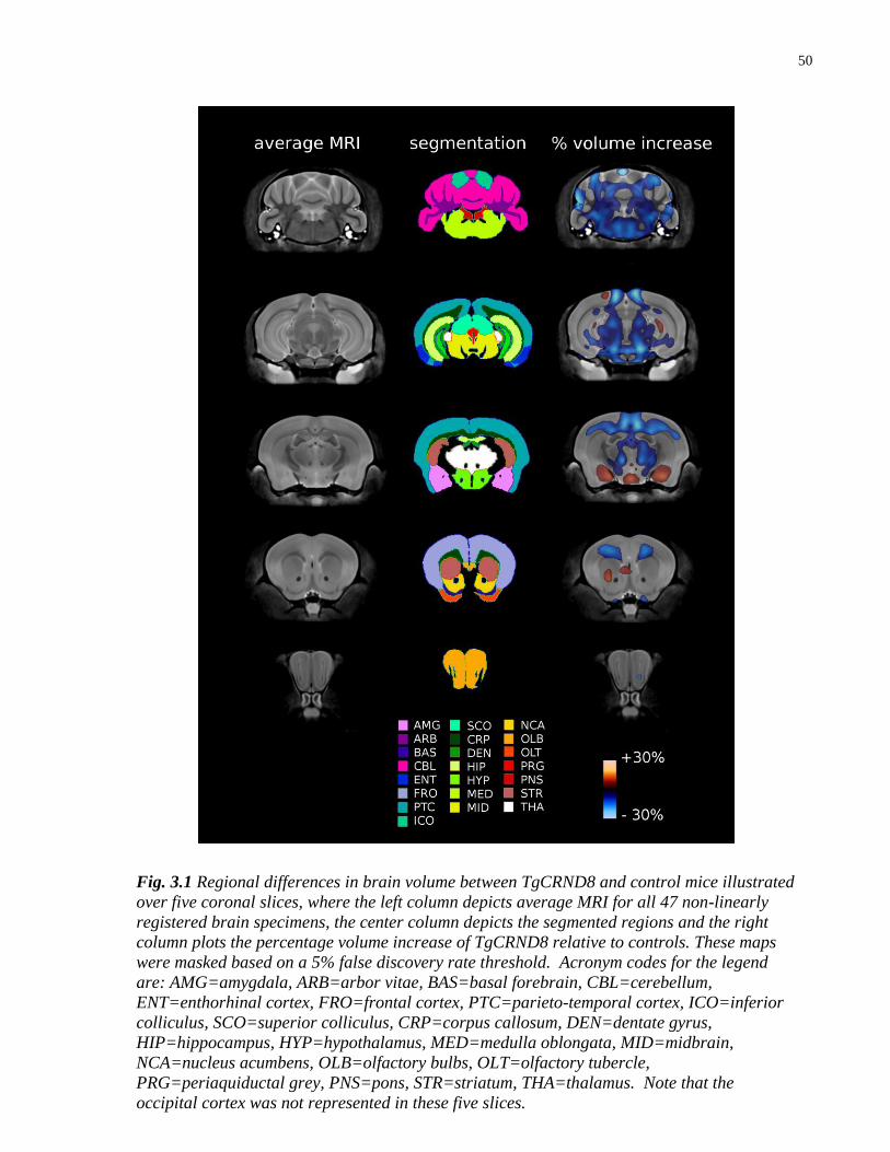
50
Fig. 3.1 Regional differences in brain volume between TgCRND8 and control mice illustrated
over five coronal slices, where the left column depicts average MRI for all 47 non-linearly
registered brain specimens, the center column depicts the segmented regions and the right
column plots the percentage volume increase of TgCRND8 relative to controls. These maps
were masked based on a 5% false discovery rate threshold. Acronym codes for the legend
are: AMG=amygdala, ARB=arbor vitae, BAS=basal forebrain, CBL=cerebellum,
ENT=enthorhinal cortex, FRO=frontal cortex, PTC=parieto-temporal cortex, ICO=inferior
colliculus, SCO=superior colliculus, CRP=corpus callosum, DEN=dentate gyrus,
HIP=hippocampus, HYP=hypothalamus, MED=medulla oblongata, MID=midbrain,
NCA=nucleus acumbens, OLB=olfactory bulbs, OLT=olfactory tubercle,
PRG=periaquiductal grey, PNS=pons, STR=striatum, THA=thalamus. Note that the
occipital cortex was not represented in these five slices.
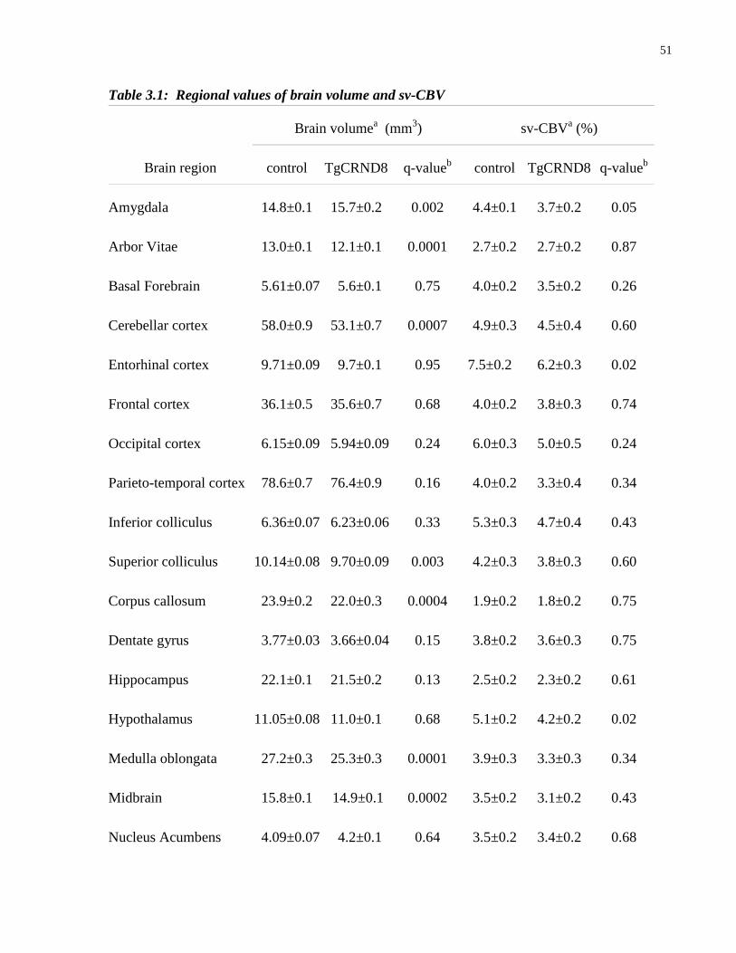
51
Table 3.1: Regional values of brain volume and sv-CBV
Brain region
Brain volumea (mm
3) sv-CBV
a (%)
control TgCRND8 q-valueb
control TgCRND8 q-valueb
Amygdala 14.8±0.1 15.7±0.2 0.002 4.4±0.1 3.7±0.2 0.05
Arbor Vitae 13.0±0.1 12.1±0.1 0.0001 2.7±0.2 2.7±0.2 0.87
Basal Forebrain 5.61±0.07 5.6±0.1 0.75 4.0±0.2 3.5±0.2 0.26
Cerebellar cortex 58.0±0.9 53.1±0.7 0.0007 4.9±0.3 4.5±0.4 0.60
Entorhinal cortex 9.71±0.09 9.7±0.1 0.95 7.5±0.2 6.2±0.3 0.02
Frontal cortex 36.1±0.5 35.6±0.7 0.68 4.0±0.2 3.8±0.3 0.74
Occipital cortex 6.15±0.09 5.94±0.09 0.24 6.0±0.3 5.0±0.5 0.24
Parieto-temporal cortex 78.6±0.7 76.4±0.9 0.16 4.0±0.2 3.3±0.4 0.34
Inferior colliculus 6.36±0.07 6.23±0.06 0.33 5.3±0.3 4.7±0.4 0.43
Superior colliculus 10.14±0.08 9.70±0.09 0.003 4.2±0.3 3.8±0.3 0.60
Corpus callosum 23.9±0.2 22.0±0.3 0.0004 1.9±0.2 1.8±0.2 0.75
Dentate gyrus 3.77±0.03 3.66±0.04 0.15 3.8±0.2 3.6±0.3 0.75
Hippocampus 22.1±0.1 21.5±0.2 0.13 2.5±0.2 2.3±0.2 0.61
Hypothalamus 11.05±0.08 11.0±0.1 0.68 5.1±0.2 4.2±0.2 0.02
Medulla oblongata 27.2±0.3 25.3±0.3 0.0001 3.9±0.3 3.3±0.3 0.34
Midbrain 15.8±0.1 14.9±0.1 0.0002 3.5±0.2 3.1±0.2 0.43
Nucleus Acumbens 4.09±0.07 4.2±0.1 0.64 3.5±0.2 3.4±0.2 0.68
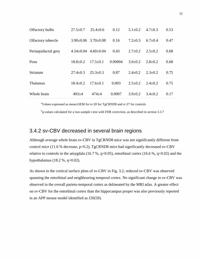
52
aValues expressed as mean±SEM for n=20 for TgCRND8 and n=27 for controls
bq-values calculated for a two-sample t-test with FDR correction, as described in section 3.3.7
3.4.2 sv-CBV decreased in several brain regions
Although average whole brain sv-CBV in TgCRND8 mice was not significantly different from
control mice (11.6 % decrease, p=0.2), TgCRND8 mice had significantly decreased sv-CBV
relative to controls in the amygdala (16.7 %, q=0.05), entorhinal cortex (16.6 %, q=0.02) and the
hypothalamus (18.2 %, q=0.02).
As shown in the cortical surface plots of sv-CBV in Fig. 3.2, reduced sv-CBV was observed
spanning the entorhinal and neighbouring temporal cortex. No significant change in sv-CBV was
observed in the overall parieto-temporal cortex as delineated by the MRI atlas. A greater effect
on sv-CBV for the entorhinal cortex than the hippocampus proper was also previously reported
in an APP mouse model identified as J20(59).
Olfactory bulbs 27.5±0.7 25.4±0.6 0.12 5.1±0.2 4.7±0.3 0.53
Olfactory tubercle 3.90±0.06 3.70±0.08 0.16 7.2±0.3 6.7±0.4 0.47
Periaquiductal grey 4.54±0.04 4.60±0.04 0.43 2.7±0.2 2.5±0.2 0.68
Pons 18.8±0.2 17.5±0.1 0.00004 3.0±0.2 2.8±0.2 0.68
Striatum 27.4±0.3 25.3±0.3 0.87 2.4±0.2 2.3±0.2 0.75
Thalamus 18.4±0.2 17.6±0.1 0.003 2.5±0.2 2.4±0.2 0.75
Whole brain 493±4 474±4 0.0007 3.9±0.2 3.4±0.2 0.17
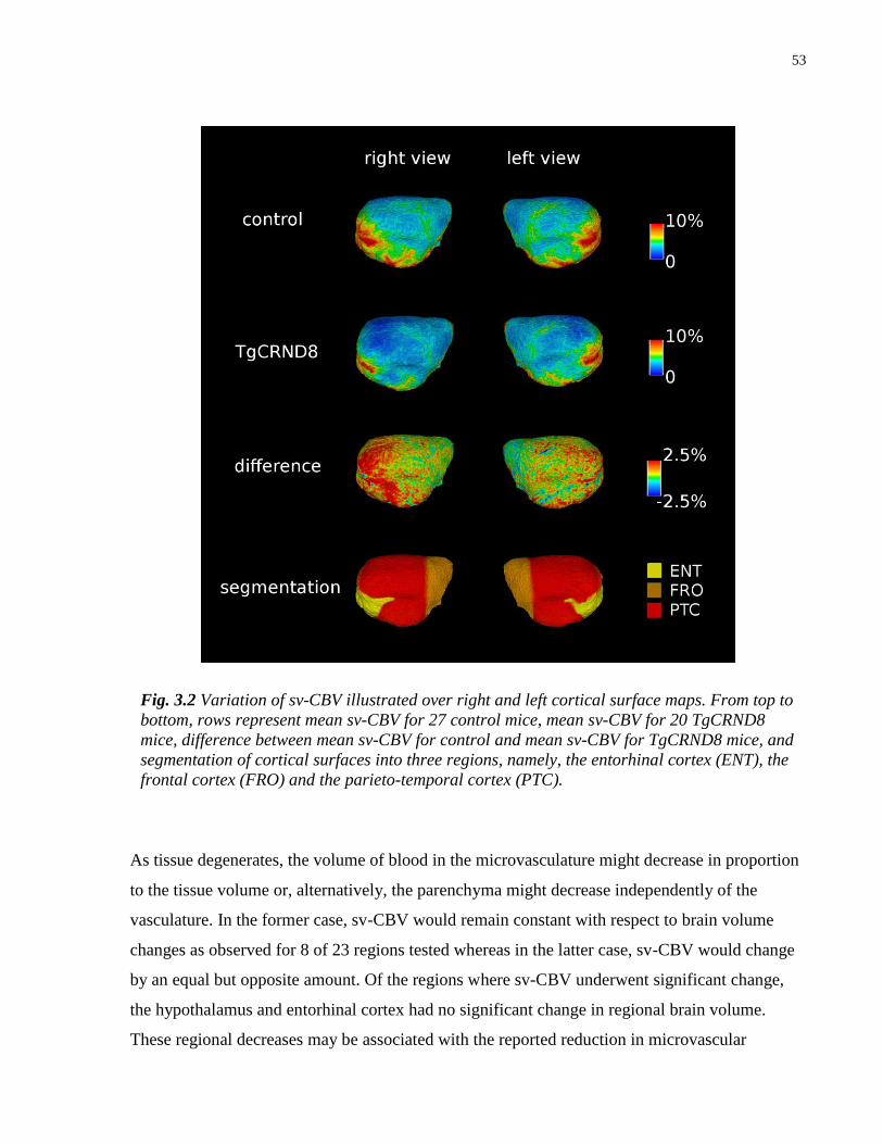
53
As tissue degenerates, the volume of blood in the microvasculature might decrease in proportion
to the tissue volume or, alternatively, the parenchyma might decrease independently of the
vasculature. In the former case, sv-CBV would remain constant with respect to brain volume
changes as observed for 8 of 23 regions tested whereas in the latter case, sv-CBV would change
by an equal but opposite amount. Of the regions where sv-CBV underwent significant change,
the hypothalamus and entorhinal cortex had no significant change in regional brain volume.
These regional decreases may be associated with the reported reduction in microvascular
Fig. 3.2 Variation of sv-CBV illustrated over right and left cortical surface maps. From top to
bottom, rows represent mean sv-CBV for 27 control mice, mean sv-CBV for 20 TgCRND8
mice, difference between mean sv-CBV for control and mean sv-CBV for TgCRND8 mice, and
segmentation of cortical surfaces into three regions, namely, the entorhinal cortex (ENT), the
frontal cortex (FRO) and the parieto-temporal cortex (PTC).
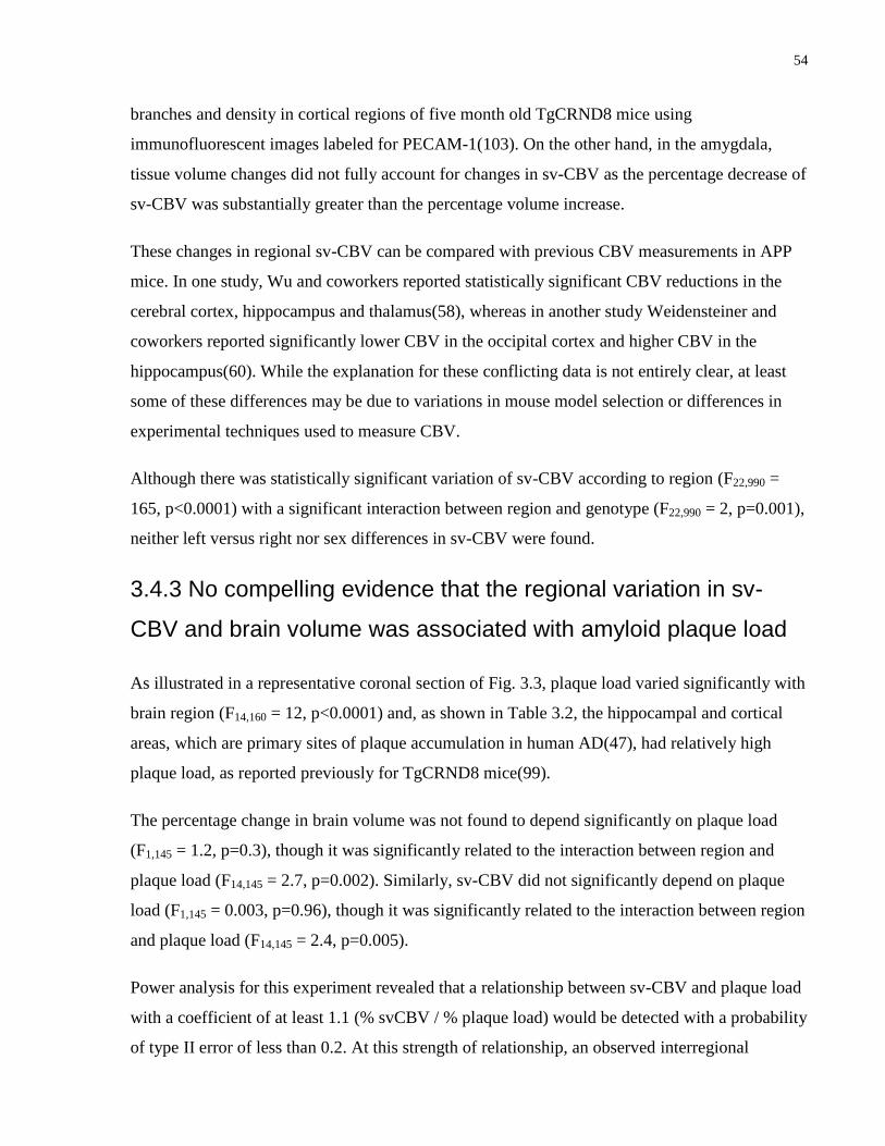
54
branches and density in cortical regions of five month old TgCRND8 mice using
immunofluorescent images labeled for PECAM-1(103). On the other hand, in the amygdala,
tissue volume changes did not fully account for changes in sv-CBV as the percentage decrease of
sv-CBV was substantially greater than the percentage volume increase.
These changes in regional sv-CBV can be compared with previous CBV measurements in APP
mice. In one study, Wu and coworkers reported statistically significant CBV reductions in the
cerebral cortex, hippocampus and thalamus(58), whereas in another study Weidensteiner and
coworkers reported significantly lower CBV in the occipital cortex and higher CBV in the
hippocampus(60). While the explanation for these conflicting data is not entirely clear, at least
some of these differences may be due to variations in mouse model selection or differences in
experimental techniques used to measure CBV.
Although there was statistically significant variation of sv-CBV according to region (F22,990 =
165, p<0.0001) with a significant interaction between region and genotype (F22,990 = 2, p=0.001),
neither left versus right nor sex differences in sv-CBV were found.
3.4.3 No compelling evidence that the regional variation in sv-
CBV and brain volume was associated with amyloid plaque load
As illustrated in a representative coronal section of Fig. 3.3, plaque load varied significantly with
brain region (F14,160 = 12, p<0.0001) and, as shown in Table 3.2, the hippocampal and cortical
areas, which are primary sites of plaque accumulation in human AD(47), had relatively high
plaque load, as reported previously for TgCRND8 mice(99).
The percentage change in brain volume was not found to depend significantly on plaque load
(F1,145 = 1.2, p=0.3), though it was significantly related to the interaction between region and
plaque load (F14,145 = 2.7, p=0.002). Similarly, sv-CBV did not significantly depend on plaque
load (F1,145 = 0.003, p=0.96), though it was significantly related to the interaction between region
and plaque load (F14,145 = 2.4, p=0.005).
Power analysis for this experiment revealed that a relationship between sv-CBV and plaque load
with a coefficient of at least 1.1 (% svCBV / % plaque load) would be detected with a probability
of type II error of less than 0.2. At this strength of relationship, an observed interregional
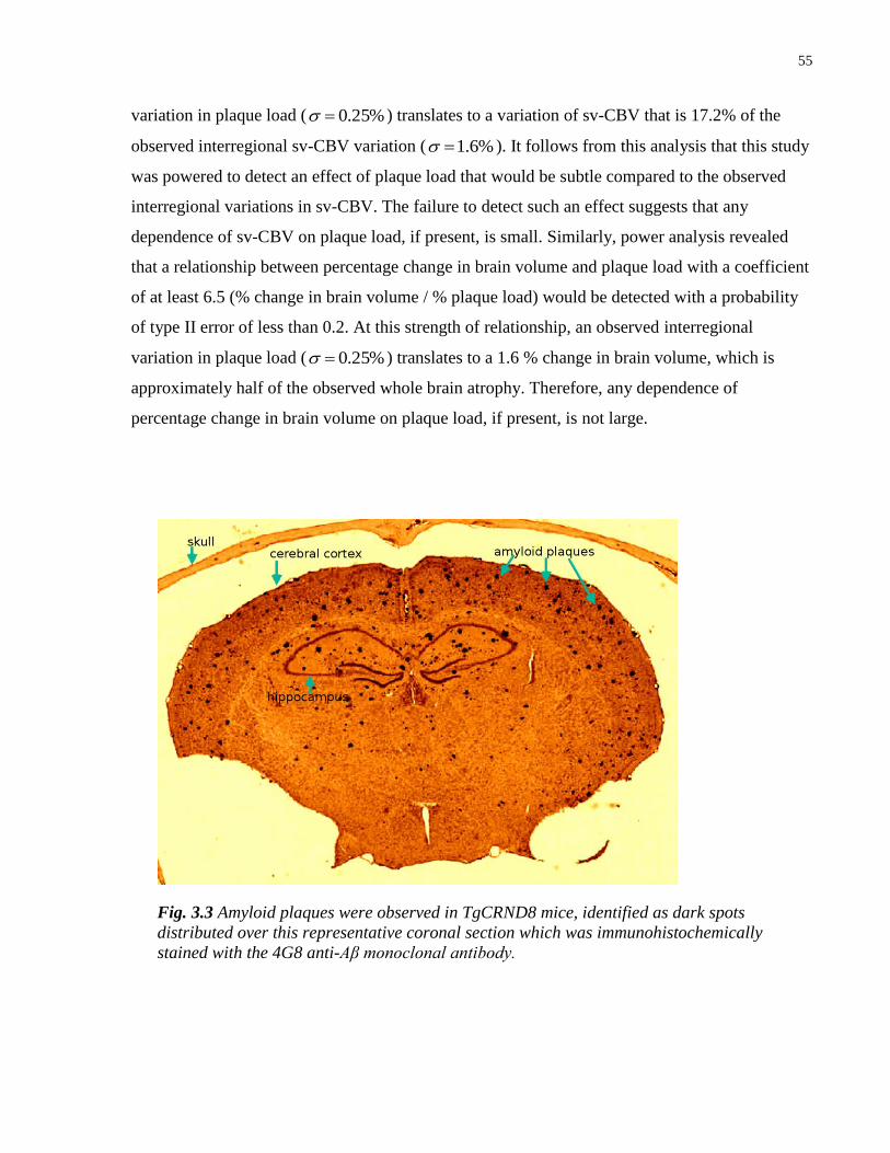
55
variation in plaque load ( %25.0 ) translates to a variation of sv-CBV that is 17.2% of the
observed interregional sv-CBV variation ( %6.1 ). It follows from this analysis that this study
was powered to detect an effect of plaque load that would be subtle compared to the observed
interregional variations in sv-CBV. The failure to detect such an effect suggests that any
dependence of sv-CBV on plaque load, if present, is small. Similarly, power analysis revealed
that a relationship between percentage change in brain volume and plaque load with a coefficient
of at least 6.5 (% change in brain volume / % plaque load) would be detected with a probability
of type II error of less than 0.2. At this strength of relationship, an observed interregional
variation in plaque load ( %25.0 ) translates to a 1.6 % change in brain volume, which is
approximately half of the observed whole brain atrophy. Therefore, any dependence of
percentage change in brain volume on plaque load, if present, is not large.
Fig. 3.3 Amyloid plaques were observed in TgCRND8 mice, identified as dark spots
distributed over this representative coronal section which was immunohistochemically
stained with the 4G8 anti-Aβ monoclonal antibody.

56
Table 3.2: Regional plaque load
Brain region Plaque loada (%) n
b
Amygdala 0.10±0.02 13
Cerebellar cortex 0.017±0.005 19
Entorhinal cortex 0.18±0.05 7
Frontal cortex 0.36±0.07 14
Occipital cortex 0.10±0.04 4
Parieto-temporal cortex 0.32±0.06 20
Corpus callosum 0.25±0.06 20
Hippocampus 0.42±0.09 19
Hypothalamus 0.016±0.006 12
Medulla oblongata 0.006±0.002 9
Midbrain 0.02±0.01 11
Olfactory bulbs 0.4±0.1 7
Pons 0.003±0.001 10
Striatum 0.025±0.005 16
Thalamus 0.07±0.02 13
aValues expressed as mean±SEM
bNumber of mice for which region was sampled
57
3.5 Conclusion
This study provides a macroscopic view of regional changes in microvasculature and brain
morphology associated with genetic differences between TgCRND8 mice and controls. While
evidence is provided of atrophy and reduced sv-CBV in several brain regions, there is no
compelling evidence that these regional changes are associated with the observed amyloid plaque
burden. Given the result of power analysis, the study design was likely to detect relationships of
even moderate strength between sv-CBV and plaque load or percentage change in brain volume
and plaque load. Therefore, the null findings are surprising since amyloid plaques, comprising
aggregates of insoluble mature fibrils of Aβ, are the most prominent histopathological
characteristic in TgCRND8 mice, which have been shown to exhibit both neuronal and
microvascular pathology. Future studies exploring the relationship between the observed
morphological changes and soluble forms of Aβ may provide further insights.
58
Chapter 4 Robust Method for 3D Arterial Spin Labeling in Mice
4.1 Foreword
The work in this chapter was previously published as:
Chugh BP, Bishop J, Zhou YQ, Wu J, Henkelman RM, Sled JG (2011), Robust method for 3D
arterial spin labeling in mice. Magnetic Resonance in Medicine. doi: 10.1002/mrm.23209
4.2 Introduction
Arterial spin labeling (ASL) provides a means for quantifying cerebral blood flow (CBF) over
mouse brain regions in a non-invasive manner. Mouse ASL permits longitudinal screening of
cerebrovascular phenotypes during the mouse lifespan of 2-3 years, which facilitates the study of
vascular factors in disease. Recent ASL applications in mice include models of stroke(111),
cerebral malaria(112), sickle cell disease(113) and Alzheimer's disease(60). There is also
considerable interest in quantifying CBF in mice for studying blood flow regulatory
mechanisms(114) and for the development of disease-specific therapies. The use of ASL in mice
is generally motivated by a desire to better understand mouse models of human disease.
Design of robust mouse ASL involves producing images with high enough resolution and signal-
to-noise-ratio (SNR) to detect important changes in regional CBF, while meeting experimental
constraints of scan time and sample size. The limits on available signal strength and gradient
performance as well as physiological differences between the species prevent a simple scaling
down of human imaging protocols for ASL from achieving satisfactory results.
Adapting amplitude-modulated continuous ASL (am-CASL) to brain size and carotid blood
velocity of mice requires optimization of the labeling gradient and B1 waveform within the given
hardware constraints. Previous work using simulation has shown that, for some combinations of
labeling parameters, inversion efficiency with am-CASL may be unstable with respect to small
variations in blood velocity(115). It is therefore necessary to map the stable regime to bracket the
anticipated blood velocity distribution for the mouse. All ASL pulse sequences are designed to
59
equalize MT signal loss in label and control images. The control experiment in am-CASL uses
an RF pulse, which is sinusoidally modulated at frequency (fm) to cause arterial spins to doubly
invert as they flow through two closely spaced inversion planes. The power and center frequency
of the RF pulse in this control experiment are matched to those used for single inversion, thereby
equalizing MT effects on brain tissue. To achieve optimal inversion efficiency, the adiabatic
inversion inequalities must be fulfilled, namely, 112 //1 BBGvT b , where v is the speed of
the inflowing spins, G is the strength of the MRI gradient during labeling, B1 is the amplitude of
the radio-frequency field and T2b is the transverse relaxation time of blood. It is also necessary to
fulfill a condition unique to am-CASL that balances the requirement for stable inversion
behavior with minimal relaxation(115), namely: 1/ 1 mfBGv . Even after satisfying these
conditions, inversion efficiency in am-CASL remains highly sensitive to velocity(116), which
requires careful slice positioning to reduce variability in CBF. With mice smaller than humans
by a factor of fifteen in each linear dimension, it is not possible to obtain high quality localizers
rapidly enough to enable accurate slice positioning by eye. Another relevant constraint is the
small size of the mouse brain since, for commonly realizable gradient strengths, the 1-2 cm
offset from the labeling plane intersecting the common carotid artery to the caudal or rostral
limits of the mouse brain, corresponds to an off-resonance frequency range of 5-20 kHz. The
associated large enhancement of T1 relaxation due to MT(117), which has been characterized for
typical CASL parameters at 7 T in rat(118), must be accounted for in CBF modeling equations to
obtain accurate CBF maps(31). Moreover, the equilibrium magnetization of the tissue is reduced
by MT. Thus, the constraints of mouse brain size and blood velocity necessitate judicious
selection of am-CASL parameters.
This study describes an experimental approach to implementing mouse am-CASL in a robust
manner. A rapid slice positioning algorithm is developed to improve the consistency of labeling
plane placement and thereby inversion efficiency. Errors in positioning the inversion plane are
evaluated. For the purpose of optimizing inversion efficiency parameters, blood velocity
distributions in the mouse common carotid arteries are characterized using pulsed-wave Doppler
ultrasound. These blood velocity data are used for simulations of inversion efficiency, while
satisfying gradient duty cycle and SAR constraints. The sensitivity of inversion efficiency to
velocity is determined. Following these developments, 3D am-CASL is implemented. The final

60
stage of this method is to calculate CBF based on an MT corrected model applicable to the high
CBF values of mice.
4.3 Materials and Methods
All animal procedures described in this study were approved by the Hospital for Sick Children
Animal Care Committee, subject to the Canadian Council for Animal Care.
4.3.1 Development of a rapid slice positioning algorithm
A slice positioning algorithm was developed which takes advantage of the conspicuity of vessel
bifurcations in rapidly acquired MRI localizer images that provide inflow contrast due to short
TR. By identifying the corresponding vessel bifurcations in a reference 3D vascular image, the
prescribed inversion plane can be mapped by landmark registration to the correct position in the
in vivo MRI coordinate system. In particular, four easily recognizable vessel landmarks with low
positional variability can be identified in mid-sagittal brain slices (as shown in Fig. 4.1a).
An MRI anatomical brain atlas was used as a reference coordinate system, with 62 labeled 3D
regions(73), prepared by averaging 20 female and 20 male C57BL/6 brain MRI images of 32 μm
isotropic resolution(74). The MRI anatomical brain atlas can be accessed at
http://www.mouseimaging.ca/technologies/C57Bl6j_mouse_atlas.html.
In this reference coordinate system, the coordinates of these four vessel landmarks were
identified using nine post-mortem micro-CT images of the cerebral vasculature of C57BL/6 mice
that had previously been co-registered to an MRI anatomical brain atlas for blood volume
measurements(93). Mean and standard deviation of each vessel landmark were calculated for the
nine brains.
In a post-mortem micro-CT cerebral vasculature specimen(93), serving as the reference 3D
vascular image, the centerlines of the common carotid arteries were traced using custom-written
software. Based on the image intensity gradient along rays perpendicular to the vessel centerline,
this software maintains equal distance from the lumen wall(72). The plane perpendicular to the
common carotid artery was selected as the inversion plane.

61
Fig. 4.1: Illustration of process of correcting for MT starting with an in vivo mid-sagittal localizer (a) with
localized vascular landmarks (1-confluence of transverse and superior sagittal sinuses; 2-confluence of
anterior cerebral artery and great cerebral vein of Galen; 3-confluence of rostral rhinal veins and superior
sagittal sinus; 4-confluence of medial orbitofrontal artery and azygos of the anterior cerebral artery) and
calculated position of inversion slice (slanted blue lines). For illustration purposes, the common carotid
artery including its bifurcation is shown overlaid on the mid-sagittal plane (b) of the MR image of a fixed
mouse (posture is not identical between a & b). Also shown is the calculated position and orientation of the
labeling plane. The mid-sagittal slice through the map of computed distance from the inversion slice is
shown in (c) and the calculated ratio of CBF (post-MT correction) to CBF (pre-MT correction) is shown in
(d). Note the systematic variation of the MT effect across the brain, decreasing from the caudal to the
rostral direction.

62
The anatomical brain atlas is oriented so that the +x direction points from medial to right lateral,
the +y direction points from caudal to rostral and the +z direction points from ventral to dorsal.
In this coordinate system, in millimeter units, the inversion plane is centered midway between
the arteries at C=[0.0,-7.0,-11.3] with normal vector of N=[0.0,0.80,0.60], as shown in Fig.4.1b.
Thus, from C and N, it follows that the equation of the inversion plane is 4y+3z+61.9=0. The
slanted blue lines in Fig.4.1a represent the components of an am-CASL double inversion, which
are equidistant and symmetric to this calculated inversion plane.
Given the in vivo locations of the landmarks (as described in section 4.3.4), the in vivo position
of the inversion plane was calculated by rigid body vascular landmark registration using a
Procrustes matching algorithm without scaling(75). This algorithm calculates the rigid body
transformation that best matches each landmark position in the reference micro-CT image to the
corresponding in vivo MRI landmarks. Using this algorithm and reference data, the placement of
the labeling plane can be computed rapidly and largely automatically by the operator at the MRI
console.
4.3.2 Analysis of errors in inversion plane positioning
A simulation was conducted to determine the extent to which uncertainty in vascular landmark
placement led to errors in inversion plane position. Ten thousand coordinates centered on the
true position of each vascular landmark were randomly generated (normal distribution with
standard deviation of 1 mm, which is the thickness of the MRI localizer scans). The rigid body
transformation that maps each simulated coordinate to the true position was computed by the
Procrustes matching algorithm without scaling. The inversion plane was transformed
accordingly. Mean positional and angular shifts of the inversion plane were determined.
4.3.3 Optimization of spin inversion efficiency parameters
The time evolution of inflowing blood magnetization was simulated in the mouse common
carotid artery. The time-velocity profile of blood was measured in the common carotid, internal
carotid and vertebral arteries of five C57BL/6 mice (body weight 20-25 g) using a VisualSonics
Vevo 2100 ultrasound scanner equipped with a 40 MHz linear array transducer. 2D Doppler
color flow imaging was used to guide each pulse wave Doppler recording in which the intercept
63
angle between the blood flow direction and the ultrasound beam was minimized to under 60° by
optimizing transducer orientation. Beam angle was accounted for in the data analysis(119).
Inversion efficiency of am-CASL, namely, (MControl – MLabel) / 2M0, was calculated in a
representative blood velocity distribution for the common carotid artery (spanning four cardiac
cycles). The Bloch equations were solved (Runge-Kutta ODE solver, Matlab) for a range of
velocities (1 to 40 cm/s) assuming a 3.1 s label pulse with T2b = 0.25 s(120) and labeling gradient
G=13 mTm-1
(constrained by maximum gradient amplitude output at 50% duty cycle). T1 effects
were neglected from the simulation. The simulations were conducted with B1 varying over the
range 1 to 20 μT and modulation frequency, fm , varying from 50 to 1000 Hz. Inversion
efficiency was calculated as an average over phase (0 to ) of the amplitude modulation at the
time the spins cross the center of the labeling plane. For each combination of parameters,
inversion efficiency was weighted by the blood velocity distribution to provide velocity-
weighted inversion efficiency.
The bias of inversion efficiency to inaccurate inversion plane orientation was evaluated by
calculating the reduction in velocity-weighted inversion efficiency corresponding to a scaling of
the velocity distribution by cos(θ). In this case, θ was the mean angular shift of the inversion
plane resulting from errors in landmark identification (as described in section 4.3.2).
4.3.4 Implementation of am-CASL in mice
3D am-CASL was performed on ten female C57BL/6 mice (20-25 g) by the following protocol:
Each mouse was scanned using a 7 T MRI scanner (Varian Inc., Palo Alto, CA, USA) with a
horizontal 30 cm inner diameter bore gradient. The mice were anesthetized with 1.2 % isoflurane
and maintained at core body temperature of 36.5±0.5°C, while being continuously monitored for
respiratory rate, temperature and heart rate(121).
To identify the vascular landmarks needed for positioning the inversion slice, a mid-sagittal
localizer image was acquired using a spoiled gradient-echo pulse sequence (TE = 4 ms, TR =
100 ms, 128 x 128 matrix, NEX=1, 90° Gaussian excitation pulse, FOV = 30 mm x 30 mm x 1
mm thick, total scan time = 13 sec). Each of the four vascular landmarks described in section
4.3.1 could be easily recognized on 1 mm thick slices.
64
Prior to each am-CASL scan, inversion efficiency was measured with inversion and imaging
planes positioned on the common carotids and separated by 4 mm. The average magnetization
over the common carotid cross-section was determined from the intra-vascular signal in three
coronal spoiled gradient-echo images of the common carotids (TE = 5.75 ms, TR = 200 ms,
NEX=4, 90° gaussian excitation pulse, matrix = 300 x 300, FOV = 30 mm x 30 mm x 1 mm
thick), one following regular labeling (B1 = 9 μT, hard pulse of 100 ms duration), the next
following sinusoidally modulation of the labeling pulse (fm=400 Hz, B1=( 2 )9 μT, 100 ms
duration) and the last by reflection of the labeling pulse (B1 = 9 μT, hard pulse of 100 ms
duration) about the imaging plane (to obtain equilibrium magnetization M0). These
measurements required a total of 12 minutes of scan time for each mouse. This protocol was
adapted from an established method of measuring inversion efficiency(122).
Flow-induced adiabatic inversion in the common carotid artery was applied using a pulse with
labeling time tL = 3.1 s, B1 = 9 μT with G = 13 mTm-1
and fm = 400 Hz using the slice positioning
algorithm described in section 4.3.1. Control and label cycles were interleaved and a post-label
delay of 500 ms was applied to reduce transit time dispersion artifacts and to clear the
intravascular signal(31). The whole brain was imaged using a 3D fast spin echo pulse sequence
(TEeff = 4 ms, TR = 6.6 s, ETL = 12, 90° hard excitation and 180° hard refocusing pulses, 60 x
96 x 80 matrix, FOV = 60 mm x 34 mm x 28 mm and NEX = 1) resulting in a total CASL scan
time of 141 min for each of the ten mice.
For estimating arterial transit time for use in CBF modeling, am-CASL was applied to a second
batch of five C57BL/6 mice at multiple post-label delays, namely, 50, 100, 200, 400, 800, and
1600 ms, while using a modified imaging matrix of 60 x 48 x 30 and FOV = 36 mm x 29 mm x
18 mm, resulting in a total scan time of 158 min for each mouse.
To provide reference tissue T1 and proton density for CBF quantification, a third batch of five
C57BL/6 mice were imaged using an inversion recovery pulse sequence with inversion times of
0.1, 0.3 and 2.0 s using a 2 ms hyperbolic secant inversion pulse and a 3D fast spin echo pulse
sequence (TEeff = 6 ms, TR = 5s, matrix = 60 x 96 x 80 with FOV = 60 mm x 34 mm x 28 mm,
90° hard excitation pulse and 180° hard refocusing pulses, ETL = 12, NEX = 1) resulting in a
total scan time of 160 min for each mouse. The T1 and proton density maps for the five mice

65
were registered to each other and to the control images of the am-CASL experiment, through a
rigid-body landmark-matching algorithm.
4.3.5 Implementation of am-CASL in mice
CBF was quantified using a single-compartment biophysical model that assumes capillaries to be
completely permeable to water (i.e permeability-surface area product = infinity), while
accounting for both transit time and magnetization transfer enhanced T1 relaxation(31; 123),
namely:
SATb
labctrl
TTTwKS
SSf
111
0 ,,,,2
, [4.1]
where:
1
1
1
1
11
1,1,1 exp1exp1expexp,,T
TT
tT
T
w
TTTTwK
SAT
LSAT
b
SATb
, [4.2]
i
n
i L
a
z
ctrl
wtM
S
nS
1
0
)(
1, [4.3]
)(1exp1)(1
L
a
zL
a
z tMT
wwtM
, [4.4]
r
ptM L
a
z )( , [4.5]
rqqR SAT 2
1 , [4.6]
and where:
RRRRRRRMRp aabarfb
b
b 0 ,
2/0 rfbbrfa
b
a RRRRRMRq , and
b
rfbb
b
rfaa RRMRRRRMRRr 00 .
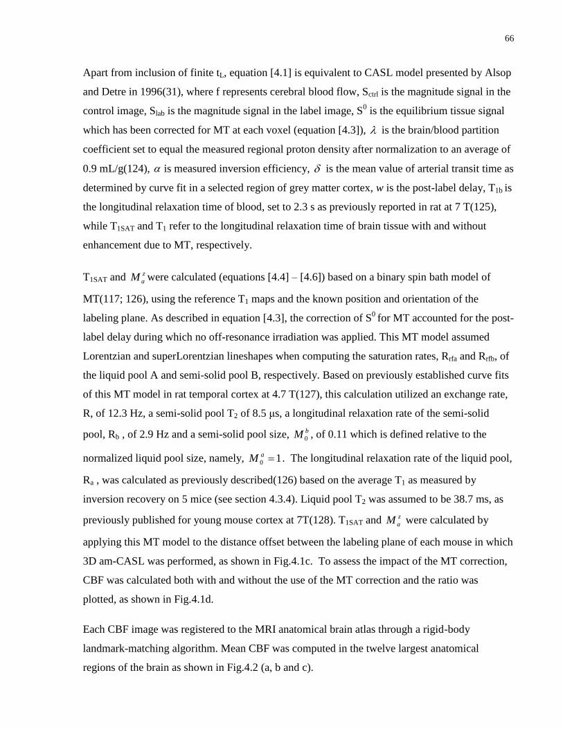
66
Apart from inclusion of finite tL, equation [4.1] is equivalent to CASL model presented by Alsop
and Detre in 1996(31), where f represents cerebral blood flow, Sctrl is the magnitude signal in the
control image, Slab is the magnitude signal in the label image, S0 is the equilibrium tissue signal
which has been corrected for MT at each voxel (equation [4.3]), is the brain/blood partition
coefficient set to equal the measured regional proton density after normalization to an average of
0.9 mL/g(124), is measured inversion efficiency, is the mean value of arterial transit time as
determined by curve fit in a selected region of grey matter cortex, w is the post-label delay, T1b is
the longitudinal relaxation time of blood, set to 2.3 s as previously reported in rat at 7 T(125),
while T1SAT and T1 refer to the longitudinal relaxation time of brain tissue with and without
enhancement due to MT, respectively.
T1SAT and z
aM were calculated (equations [4.4] – [4.6]) based on a binary spin bath model of
MT(117; 126), using the reference T1 maps and the known position and orientation of the
labeling plane. As described in equation [4.3], the correction of S0
for MT accounted for the post-
label delay during which no off-resonance irradiation was applied. This MT model assumed
Lorentzian and superLorentzian lineshapes when computing the saturation rates, Rrfa and Rrfb, of
the liquid pool A and semi-solid pool B, respectively. Based on previously established curve fits
of this MT model in rat temporal cortex at 4.7 T(127), this calculation utilized an exchange rate,
R, of 12.3 Hz, a semi-solid pool T2 of 8.5 μs, a longitudinal relaxation rate of the semi-solid
pool, Rb , of 2.9 Hz and a semi-solid pool size, bM 0 , of 0.11 which is defined relative to the
normalized liquid pool size, namely, 10 aM . The longitudinal relaxation rate of the liquid pool,
Ra , was calculated as previously described(126) based on the average T1 as measured by
inversion recovery on 5 mice (see section 4.3.4). Liquid pool T2 was assumed to be 38.7 ms, as
previously published for young mouse cortex at 7T(128). T1SAT and z
aM were calculated by
applying this MT model to the distance offset between the labeling plane of each mouse in which
3D am-CASL was performed, as shown in Fig.4.1c. To assess the impact of the MT correction,
CBF was calculated both with and without the use of the MT correction and the ratio was
plotted, as shown in Fig.4.1d.
Each CBF image was registered to the MRI anatomical brain atlas through a rigid-body
landmark-matching algorithm. Mean CBF was computed in the twelve largest anatomical
regions of the brain as shown in Fig.4.2 (a, b and c).
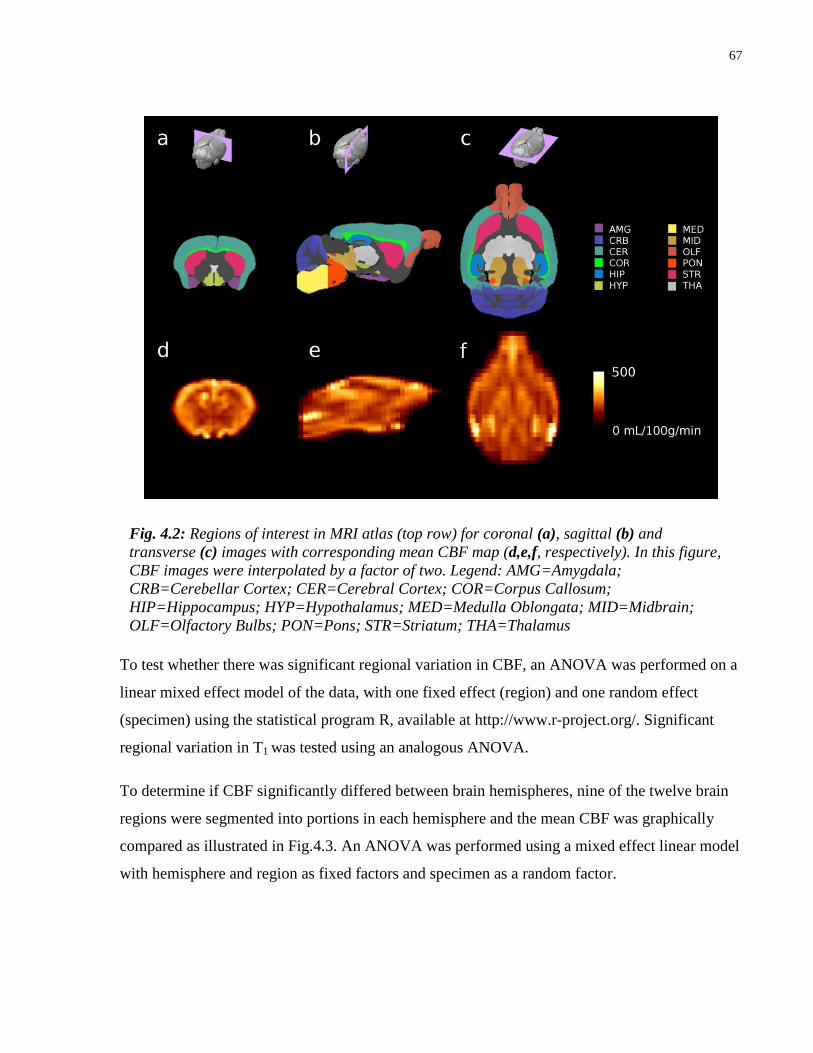
67
To test whether there was significant regional variation in CBF, an ANOVA was performed on a
linear mixed effect model of the data, with one fixed effect (region) and one random effect
(specimen) using the statistical program R, available at http://www.r-project.org/. Significant
regional variation in T1 was tested using an analogous ANOVA.
To determine if CBF significantly differed between brain hemispheres, nine of the twelve brain
regions were segmented into portions in each hemisphere and the mean CBF was graphically
compared as illustrated in Fig.4.3. An ANOVA was performed using a mixed effect linear model
with hemisphere and region as fixed factors and specimen as a random factor.
Fig. 4.2: Regions of interest in MRI atlas (top row) for coronal (a), sagittal (b) and
transverse (c) images with corresponding mean CBF map (d,e,f, respectively). In this figure,
CBF images were interpolated by a factor of two. Legend: AMG=Amygdala;
CRB=Cerebellar Cortex; CER=Cerebral Cortex; COR=Corpus Callosum;
HIP=Hippocampus; HYP=Hypothalamus; MED=Medulla Oblongata; MID=Midbrain;
OLF=Olfactory Bulbs; PON=Pons; STR=Striatum; THA=Thalamus

68
A power analysis for a t-test was conducted (two-sided, two-sample, probability of type I error =
0.05, probability of type II error = 0.2) using the measured variation in hippocampal CBF as a
representative region of interest.
All computed parameters were expressed as mean ± standard-error-of-the-mean (SEM) unless
stated otherwise.
Fig. 4.3: Bilateral symmetry of CBF for nine brain regions (amygdala, cerebellar cortex,
cerebral cortex, corpus callosum, hippocampus, hypothalamus, olfactory bulbs, striatum,
thalamus) illustrated by plotting left versus right portion of CBF. Error bars represent ±SEM
for n=10. For reference, the line of symmetry is indicated.

69
Fig. 4.4: (a) Dependence of velocity-weighted inversion efficiency on B1 for an am-CASL
experiment. Simulation parameters were G = 13 mTm-1
and fm = 400 Hz. Velocity-
weighted inversion efficiency reaches its peak of 0.87 at B1 = 9 μT. (b) Dependence of
velocity-weighted inversion efficiency on fm for an am-CASL experiment. Simulation
parameters were G=13 mTm-1
, B1=9μT. (c) Dependence of longitudinal magnetization
on blood velocity for control pulse (dashed curve) and labeling pulse (solid curve) in an
am-CASL experiment with G =13 mTm-1
, B1 = 9 μT and fm = 400 Hz. (d) Dependence of
inversion efficiency (thick curve) on blood velocity. Blood velocity distribution is also
shown (thin curve). Simulation parameters were G = 13 mTm-1
, B1 = 9μT and fm = 400
Hz.
70
4.4 Results
The simulation of inversion efficiency in am-CASL provided an optimized parameter set
corresponding to a gradient of 13 mTm-1
. As illustrated in Fig.4.4a, the velocity-weighted
inversion efficiency peaked at B1 = 9 μT and reached a maximum value of 0.87. The effect of
varying modulation frequency, illustrated in Fig.4.4b, was to increase inversion efficiency until
saturation after 300 Hz. Fig.4.4c illustrates the dependence of longitudinal magnetization on
velocity for the labeling and control experiment. Despite the oscillatory nature of the
magnetization in the control experiment at high velocities and the steep drop at low velocities,
there is a relatively flat region for both control and label magnetization in the range of 5 and 15
cm/s. Further, in Fig.4.4d, which plots the dependence of inversion efficiency on velocity
alongside a representative velocity distribution for the common carotid artery, it is apparent that
the inversion efficiency is relatively constant for the velocity window that contains the bulk of
the velocity distribution. This, of course, is non-coincidental as the optimized parameter-set
from the simulation (B1 = 9 μT, fm = 400Hz and G = 13 mTm-1
) were derived from the pulse-
wave Doppler ultrasound measurements. Similar time averaged mean velocities were observed in
all feeding arteries to the brain, with mean±standard-deviation (SD) of 12±1 cm/s, 12±2 cm/s,
14±3 cm/s, 11±2 cm/s, 10±2 cm/s, 11±1 cm/s for the left common carotid artery, right common
carotid artery, left internal carotid artery, right internal carotid artery, left vertebral artery and
right vertebral artery, respectively.
Analysis of errors in inversion plane positioning determined that, in the event of a large
variability in landmark positioning in the range of 1 mm per landmark, the mean positional and
angular shifts of the inversion plane were 2.4 mm and 18.6°, respectively. Misalignment of this
magnitude would result in an inversion efficiency loss of 0.5 %. The selected vascular
landmarks, based on micro-CT images, were found to have low inter-mouse variation (standard
deviation of 0.19 mm).
Statistically significant differences in CBF (F11,99 = 19.28, p<0.0001) and T1 (F11,44=176.31,
p<0.0001) were observed over the twelve regions examined, with values listed in Table 4.1. T1
for the total brain was 1.53± 0.01 s. Based on the MT model, the group average T1SAT and
)( wtM L
a
z were 0.57 s and 0.48, respectively. CBF for brain was found to be 219±6
ml/100g/min, based on the measured inversion efficiency of 0.67 ± 0.03 and the fitted arterial
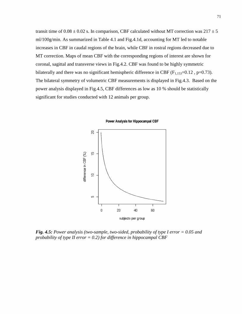
71
transit time of 0.08 ± 0.02 s. In comparison, CBF calculated without MT correction was 217 ± 5
ml/100g/min. As summarized in Table 4.1 and Fig.4.1d, accounting for MT led to notable
increases in CBF in caudal regions of the brain, while CBF in rostral regions decreased due to
MT correction. Maps of mean CBF with the corresponding regions of interest are shown for
coronal, sagittal and transverse views in Fig.4.2. CBF was found to be highly symmetric
bilaterally and there was no significant hemispheric difference in CBF (F1,153=0.12 , p=0.73).
The bilateral symmetry of volumetric CBF measurements is displayed in Fig.4.3. Based on the
power analysis displayed in Fig.4.5, CBF differences as low as 10 % should be statistically
significant for studies conducted with 12 animals per group.
Fig. 4.5: Power analysis (two-sample, two-sided, probability of type I error = 0.05 and
probability of type II error = 0.2) for difference in hippocampal CBF
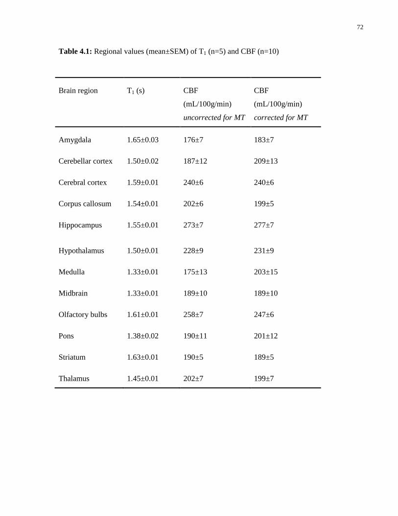
72
Table 4.1: Regional values (mean±SEM) of T1 (n=5) and CBF (n=10)
Brain region T1 (s) CBF
(mL/100g/min)
uncorrected for MT
CBF
(mL/100g/min)
corrected for MT
Amygdala 1.65±0.03 176±7 183±7
Cerebellar cortex 1.50±0.02 187±12 209±13
Cerebral cortex 1.59±0.01 240±6 240±6
Corpus callosum 1.54±0.01 202±6 199±5
Hippocampus 1.55±0.01 273±7 277±7
Hypothalamus 1.50±0.01 228±9 231±9
Medulla 1.33±0.01 175±13 203±15
Midbrain 1.33±0.01 189±10 189±10
Olfactory bulbs 1.61±0.01 258±7 247±6
Pons 1.38±0.02 190±11 201±12
Striatum 1.63±0.01 190±5 189±5
Thalamus 1.45±0.01 202±7 199±7
73
4.5 Discussion
Selecting a mouse ASL protocol involves making a series of choices. First, the protocol for
spatially-selective labeling can either be Pulsed ASL (PASL), where blood water magnetization
is labeled in a large slab proximal to the imaging slice, or Continuous ASL (CASL), where blood
water magnetization is continuously labeled as it flows through a plane intersecting the carotid
arteries. CASL was selected for this work due to its inherently higher signal strength(129).
Second, an image readout portion of the protocol must be selected. This study focused on a 3D
approach to ASL. By imaging the entire brain, one can screen mutant mice for regional CBF
phenotypes, while permitting regions of interest to be defined retrospectively. Relative to single
slice imaging, whole brain imaging also facilitated automated registration to an MRI atlas and
subsequent data mining. Furthermore, 3D imaging has the advantage that overlap of slice
excitation profiles and saturation of arterial blood by proximal slice excitation can be avoided.
Third, a choice must be made between implementing CASL using a separate coil for labeling or
using only the imaging coil(130). Single-coil CASL was implemented to avoid the need for
additional hardware. This choice forces one to choose a strategy to control for magnetization
transfer (MT). This study utilized the am-CASL labeling protocol(34), which places lower
demands on the MRI gradient than pseudo-continuous ASL while maintaining high inversion
efficiency(30). Moreover, relative to the simultaneous proximal and distal irradiation method,
am-CASL provides more consistent control of MT effects over the entire brain(9).
A slice positioning algorithm was developed to position the labeling plane perpendicular to the
common carotid arteries to ensure that the apparent velocity through the plane is high enough to
avoid inefficiency associated with low velocity. In the mouse, this slice positioning algorithm is
robust, as demonstrated by the simulated reduction of only 0.5 % in inversion efficiency
associated with the hypothetical case of large variability in landmark selection. Furthermore, this
method is easy to implement when labeling blood in the long and parallel common carotid
arteries. By utilizing the inversion plane position recommended in this study, comparable
inversion efficiency is expected for the vertebral and common carotid arteries, given their similar
orientation and velocity distribution. Variation in neck posture between micro-CT and MRI
scans was reduced by the use of an anatomically-moulded sled during MRI scanning and by
careful positioning during fixation in the previous micro-CT study. Observed variation in the
angulation of the common carotids among micro-CT specimens was approximately 10 º,
74
suggesting that any systematic effect of postural differences on inversion efficiency was small
compared to other factors. Labeling of the common carotid arteries is preferable to the internal
carotid arteries since MT enhancement of T1 in the vicinity of the labeling plane will reduce the
magnitude of the difference signal and, hence, reduce the precision of the CBF estimate.
Pulsed Doppler ultrasound measurements provide an efficient method to characterize common
carotid blood velocity in mice. Furthermore, the calculated inversion parameters were robust
with respect to blood velocity variation. This suggests that re-measurement of blood velocity
should only be necessary in cases where very large changes in carotid velocity are expected (e.g.
a stroke model) or where measured inversion efficiency is sub-optimal. Although the difference
between measured and simulated inversion efficiency may be partly explained based on the
known bias in favor of measuring slower moving spins(131), another potential factor is T2b.
There is considerable variation in the literature on measured T2b(120; 132–134), which is likely
related to both physiological factors such as oxygenation and hematocrit as well as the timescale
over which refocusing occurs. Short refocusing intervals lead to significantly larger T2b
estimates(135). The relatively rapid transition that occurs during am-CASL inversion can be
treated as a short refocusing period and justifies the use of longer T2b values when calculating
inversion efficiency. For comparison, inversion efficiency for a shorter T2b of 70 ms was
estimated at 0.64 as compared to 0.87 with a T2b of 250ms. A benefit of utilizing measured
inversion efficiency in calculations of CBF is to reduce variability due to individual velocity
differences. Although the mean velocity as measured by ultrasound was consistent across the
group, it is still possible to find individual mice with atypical velocity distributions, which can
ultimately impact inversion efficiency.
As depicted in Fig.4.2 (d,e,f), the described 141 minute CASL protocol provided high enough
SNR to reveal blood flow contrast between neighbouring brain structures such as the cerebral
cortex and surrounding white matter. Based on recorded heart rate, respiration and temperature,
physiological parameters were stable throughout each CASL scan. This is consistent with a
previous study which found that under similar anesthesia conditions, CBF was stable over 70
minutes(136). Where necessary it should be possible to reduce scan times by using a shorter
labeling period, leading to lower SNR. The reduced SNR may, however, increase variability in
the CBF data, which may in turn compromise statistical power. Additional SNR could be gained
75
by reducing post-label delay to significantly less than 500ms, which was an overly conservative
selection given that the measured arterial transit time was only 80ms.
As shown in Table 4.1, the observed regional CBF values were larger in gray than white matter
structures. Brain stem structures such as the medulla, pons and midbrain, which have a mixture
of gray and white matter, tended to have only slightly lower CBF than major gray matter regions
such as the cerebral cortex. A diverse range of CBF values in mice have been reported under
similar experimental conditions. For example, three single-coil CASL studies on horizontally
loaded mice maintained at 37 ºC and anesthetized with average isoflurane concentration
(mean±SD) of 1.3±0.6 %, reported whole brain CBF (mean±SD) of 208±12 ml/100g/min(137),
215±27 ml/100g/min(114), and 165±13 ml/100g/min(60). The whole brain MT corrected CBF
(mean±SD) reported in this study of 219±18 ml/100g/min, while similar to other single-coil
CASL studies, is higher than that reported by autoradiography(138; 139). While the explanation
for this difference between autoradiography and CASL is presently unclear, a similar
discrepancy has been previously reported for single-coil CASL studies applied to the rat
brain(140). Differences in body temperature(136), anesthesia level(141) and subject
orientation(114) may account for some of the reported differences in CBF.
The need to account for MT enhancement of T1 could be avoided by using a much higher
gradient (> 200 mTm-1
) or much lower B1. The former option is, however, challenging due to
hardware overheating limits, whereas the latter option may restrict the inversion efficiency to
impractically low values. In this study, CBF was modeled to account for MT effects, which has
not been routinely applied in mouse ASL studies. While local CBF values were affected by the
MT correction, the relatively minor global effect of the correction may partly explain why this
effect has been underreported in past mouse ASL studies. As shown in Fig.4.1d and tabulated in
Table 4.1, the observed pattern of variation of the MT effect on CBF is dependent on position
and orientation of the labeling plane. MT effects were accounted for in the CBF modeling to
avoid having to measure this effect for each mouse. To improve accuracy of MT modeling, this
study utilized T1 and T2 of the liquid pool based on mouse brain data at 7 T. Four parameters in
the binary spin bath model were based on 4.7 T rat brain data, namely, exchange rate, semi-solid
pool size, semi-solid pool T1 and semi-solid pool T2. The accuracy of this extrapolation of MT
parameters to 50% higher field strength is supported by a study that compared these MT
parameters over a wider field strength range in three concentrations of agar and reported little
76
variation(126). Furthermore, CBF as computed by equation [4.1] was found to be relatively
insensitive to substantial variations in those MT parameters that were adopted from 4.7 T. It is,
however, possible that direct measurement of T1SAT and the equilibrium tissue signal may further
refine CBF modeling(118; 142).
Two-compartment CBF models have been proposed as an enhancement for human ASL. The
single-compartment model applied in this study assumes complete permeability of the capillary
wall to water exchange (i.e. PS=infinity). Applying the two-compartment model, namely, the
fast flow solution proposed by Parkes and Tofts(23), to data in this study using a PS reported for
rat cerebral cortex of 3.3 ml/g/min(143), a blood volume of 0.04(36) and a blood water content
of 0.7(144), provided a whole brain CBF estimate of 221 mL/100g/min, which is within 1 % of
the value computed using the single-compartment model. In fact, the single and two-
compartment models differed by less than 10 % provided that PS was selected to be over 1.7
ml/g/min. This suggests that the single-compartment model is realistic for use in computing
mouse brain CBF.
The development of robust am-CASL in mice was motivated by a desire to pursue large-scale
applications that would greatly benefit from high-throughput protocols. As demonstrated by the
power analysis, it is feasible to detect small differences in CBF when screening moderate
numbers of mutant mice.
77
Chapter 5 Discussion and Conclusion
5.1 Summary
This thesis developed and tested techniques for measuring two perfusion-related metrics in
mouse brain regions, namely, CBV and CBF using micro-CT and ASL, respectively. These
techniques could lead to improved characterization of vascularity in models of neurological
diseases.
Chapter 2 described the development of a technique to measure CBV in the mouse brain using
micro-CT. Key features of the described method were vascular perfusion under controlled
pressure, registration of the micro-CT images to an MRI anatomical brain atlas and re-scaling of
micro-CT intensities to CBV units with selectable exclusion of major vessels. Histological
validation of the vascular perfusion showed that the average percentage of vessels filled was
93±3%. Comparison of thirteen brain regions in nine mice revealed significant differences in
CBV between regions (p<0.0001), while cortical maps showed that primary visual and auditory
areas had higher CBV than primary somatosensory areas.
Chapter 3 described a study in the TgCRND8 model of AD in which regional patterns of brain
volume and sv-CBV were measured with MRI and micro-CT, respectively. These metrics were
compared with amyloid plaque load as detected by immunohistochemistry. Widespread brain
atrophy was observed when comparing data collected on twenty TgCRND8 mice and twenty-
seven controls, including significant overall brain volume loss (4.0%, p=0.0007), with greater
atrophy in caudal brain regions. Additionally, significantly reduced svCBV was observed in the
amygdala (17.4%, p=0.04), the entorhinal cortex (17.5%, p=0.01) and the hypothalamus (18.3%,
p=0.01). There was no compelling evidence that regional variation in sv-CBV or brain volume
was associated with amyloid plaque load.
78
Chapter 4 described a technique for robust mapping of CBF over 3D brain regions using am-
CASL. To provide physiological data for CBF modeling, the carotid artery blood velocity
distribution was characterized using pulsed-wave Doppler ultrasound. These blood velocity
measurements were utilized in simulations that optimize inversion efficiency for parameters
meeting MRI gradient duty cycle constraints. A rapid slice positioning algorithm was developed
and evaluated to provide accurate positioning of the labeling plane. To account for enhancement
of T1 due to magnetization transfer, a binary spin bath model of MT was utilized to provide a
more accurate estimate of CBF. A study conducted on ten mice provided highly reproducible
inversion efficiency (0.67±0.03), statistically significant variation in CBF over 12 brain regions
(p<0.0001) and a whole brain CBF of 219±6 ml/100g/min.
The sections below provide a discussion of further technical considerations for the perfusion-
related metrics developed and tested. The material covered in this chapter extends the discussion
beyond that in the body of this thesis and considers future directions.
5.2 Further technical considerations
Several lessons were learned during development of the perfusion protocol in chapter 2,
described as follows: (i)- administration of the anticoagulant, heparin, improved consistency of
perfusions, but was best limited at 10 IU/ g of mouse body weight to avoid excessive mouse
bleeding; (ii)- a pilot study conducted in preparation for CBV measurements, testing the effect of
a standard vasodilator, acepromazine maleate, on a small sample of mice, provided evidence of
higher success rate for perfusions; (iii)- initial attempts to cannulate all four feeding arteries to
the brain were abandoned due to difficulty in accessing the arteries without causing irrecoverable
structural damage; attempts to cannulate the aorta at different locations were complicated either
by excessive bleeding of neighboring vessels of the thymus gland or technical difficulties in
efficient reproduction of the cannulation; (iv)- during clearance of the blood with warm
heparinized phosphate buffered saline, at pressures significantly greater than 50 mmHg, the
replacement of blood was not isovolumetric and there was evidence of edema in the form of
swollen tissues; (v)- during Microfil infusion, pressures exceeding 180 mmHg were sometimes
accompanied by burst vessels in the cerebral vasculature; on the other hand, infusion pressures
79
under 120 mmHg were found to reduce consistency of perfusions; and, (vi)- of the several
methods for sealing off the venous outlet vessels, including cauterization, ligation and adhesion,
the simple approach of using super glue adhesive was found to be the most reproducible.
Following these considerations, the procedure described in chapter 2, provided a high percentage
of quality perfusions, yielding approximately 85% success rate for the perfusions described in
this thesis. Major lines of evidence that support the accuracy of CBV determination using this
protocol included the observations: (i)- that 93 ± 3% of vessels were found to be filled with
Microfil as assessed histologically; this may have been underestimated due to minor
displacement of Microfil fragments during slide preparations, or alternatively, may be related to
a small percentage of unperfused capillaries; (ii)- that the completeness of Microfil perfusion, as
assessed histologically, did not significantly differ between the locations examined; (iii)- that the
respective ratio of CBV in cortical gray matter to white matter (corpus callosum) was 2.5:1,
which is supported by a past study on the rat(35); and, (iv)- that the pattern of variation of sv-
CBV through cortical depth was similar to the previously observed microvessel density variation
in rats and humans. It is worth noting that points (ii) and (iii) also support that the lower values
of CBV reported in certain regions were truly related to differences in vessel density and not just
a filling artifact.
Other possibilities for obtaining validation of CBV measurements have been proposed in the
literature. For example, in an experimental protocol, MRI bolus tracking measurements of
relative CBV were correlated with CBV estimated using stereological principles applied to
fractional vessel area measurements on frozen sections of Microfil-perfused rat brains(28). A
prerequisite to obtaining sound measures of CBV with histological validation is that the contrast
agent must remain stable within the vasculature. In my experience, frozen sectioning of Microfil-
perfused mouse brain specimens did not consistently retain the Microfil segments within the
vessel lumen to meet the standard needed for histological validation. The Microfil was, however,
found to be retained in the vessels upon switching from frozen to paraffin embedding, although
the two day paraffin embedding protocol applied in this thesis causes Microfil to shrink by 60-
85%, as determined by comparison of micro-CT images of cured pieces of Microfil before and
after applying the protocol. Thus, although the paraffin embedding protocol was useful for
measuring the proportion of vessels filled with Microfil, the large amount of observed shrinkage
of Microfil made it difficult to estimate CBV reliably from the histological images. While other

80
imaging options, such as ones described in chapter 1, remain feasible alternatives to using micro-
CT mapping of CBV, each is not without its own technical challenges.
The co-registration of micro-CT and MRI images allowed the strengths of both modalities to
synergize for calculation of CBV. Micro-CT images provided excellent contrast of vessel
lumen, but relatively poor contrast of soft tissue boundaries. On the other hand, the T2-weighted
anatomical MRI images provided superior contrast for delineating soft tissue boundaries, but
relatively limited vessel contrast. Thus, by using images from both modalities, it was possible to
obtain the resulting measure of micro-CT defined volume of vasculature per each MRI defined
volume of region. To accomplish this task, vascular landmark registration was developed in
chapter 2 and subsequently further refined and applied in chapter 3. The main distinction in the
registration procedure of the studies of chapter 2 and 3 was the increase in the number of
landmarks utilized, from 4 to 20, respectively. The ability to accurately select more landmarks
became possible with the acquisition of 3D high resolution MRI images of each Microfil-
perfused specimen in the study of chapter 3. There was no evidence of inaccurate registration
associated with observed chemical shift of cured Microfil (4.0±0.3 ppm), as viewed in the MRI
images. A drawback of manually selecting more landmarks is the longer time investment needed.
In my experience, the manual work involved in tagging 20 landmarks per pair of MRI and
micro-CT images could be accomplished in half an hour per specimen after initially learning the
routine.
Although the whole brain svCBV (mean±SEM) was similar for the wildtype mice in the studies
described in chapters 2 and 3, namely, 4.4±0.3 % and 3.9±0.2 %, respectively, considerable
regional differences in svCBV were observed, as illustrated in Fig.5.1. Based on a separate
analysis, sex differences among mice in the studies could not account for these differences. The
improved registration method of chapter 3 relative to chapter 2 may partly account for the
reduced white-matter svCBV values by mitigating partial volume effects. Variability of vascular
architecture has been previously reported for several mouse inbred strains(145), suggesting that
genetic background may account for differences in cerebral vascular anatomy. It is possible that
these differences extend to the microvasculature and are reflected in the svCBV differences in
Fig.5.1.
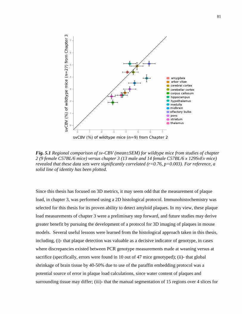
81
Fig. 5.1 Regional comparison of sv-CBV (mean±SEM) for wildtype mice from studies of chapter
2 (9 female C57BL/6 mice) versus chapter 3 (13 male and 14 female C57BL/6 x 129SvEv mice)
revealed that these data sets were significantly correlated (r=0.76, p=0.003). For reference, a
solid line of identity has been plotted.
Since this thesis has focused on 3D metrics, it may seem odd that the measurement of plaque
load, in chapter 3, was performed using a 2D histological protocol. Immunohistochemistry was
selected for this thesis for its proven ability to detect amyloid plaques. In my view, these plaque
load measurements of chapter 3 were a preliminary step forward, and future studies may derive
greater benefit by pursuing the development of a protocol for 3D imaging of plaques in mouse
models. Several useful lessons were learned from the histological approach taken in this thesis,
including, (i)- that plaque detection was valuable as a decisive indicator of genotype, in cases
where discrepancies existed between PCR genotype measurements made at weaning versus at
sacrifice (specifically, errors were found in 10 out of 47 mice genotyped); (ii)- that global
shrinkage of brain tissue by 40-50% due to use of the paraffin embedding protocol was a
potential source of error in plaque load calculations, since water content of plaques and
surrounding tissue may differ; (iii)- that the manual segmentation of 15 regions over 4 slices for
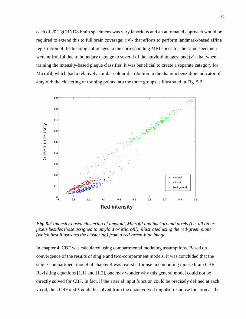
82
each of 20 TgCRND8 brain specimens was very laborious and an automated approach would be
required to extend this to full brain coverage; (iv)- that efforts to perform landmark-based affine
registration of the histological images to the corresponding MRI slices for the same specimen
were unfruitful due to boundary damage to several of the amyloid images; and (v)- that when
training the intensity-based plaque classifier, it was beneficial to create a separate category for
Microfil, which had a relatively similar colour distribution to the diaminobenzidine indicator of
amyloid; the clustering of training points into the three groups is illustrated in Fig. 5.2.
Fig. 5.2 Intensity-based clustering of amyloid, Microfil and background pixels (i.e. all other
pixels besides those assigned to amyloid or Microfil), illustrated using the red-green plane
(which best illustrates the clustering) from a red-green-blue image.
In chapter 4, CBF was calculated using compartmental modeling assumptions. Based on
convergence of the results of single and two-compartment models, it was concluded that the
single-compartment model of chapter 4 was realistic for use in computing mouse brain CBF.
Revisiting equations [1.1] and [1.2], one may wonder why this general model could not be
directly solved for CBF. In fact, if the arterial input function could be precisely defined at each
voxel, then CBF and λ could be solved from the deconvolved impulse-response function as the
83
maximum value and area under the curve, respectively. In this case, no assumptions about
intercompartment exchange mechanisms would be needed. Another benefit of developing
deconvolution methods is the ability to extract greater amounts of physiological information,
such as the regional variation of PS for water.
The deconvolution approach is, however, highly noise sensitive and requires knowledge of the
complete shape of both the arterial input function and the tissue concentration-time curve(8; 9).
Thus, the arterial and tissue concentration-time curves would have to be precisely acquired at
high temporal resolution. CASL, which was selected for this thesis to provide maximal SNR for
mouse imaging, only provides a single time point measurement without information on shape of
the dynamic tracer concentration curves and is, therefore, not suited for this approach. In human
ASL, recently proposed pulse sequences that rapidly acquire data at multiple time points, while
providing a well defined bolus, may lead to feasible options for using deconvolution in mouse
ASL studies(146).
It is worth noting that even if deconvolution methods were applied to ASL data, they would not
provide CBV, since water is a diffusible tracer with a volume of distribution equal to its partition
coefficient, which is an order of magnitude larger than CBV. Therefore, an intravascular tracer
would be required to solve for both CBF and CBV.
Another key assumption in CBF modeling is that the labeled blood water arrives in each voxel
by uniform plug flow. In reality, the shape of the arterial input will undergo dispersion as the
flow profile is not exactly plug flow, but more like an intermediate mixture of parabolic and plug
flow(14). It is unclear whether accounting for dispersion during the relatively short 80ms arterial
transit period of mice will substantially improve measurement of CBF. To be useful to
phenotyping applications, any such correction would have to be generalizable to account for
dispersion in mouse models of vascular disease.
As discussed in chapter 4, side effects of MT on the ASL experiment could be diminished if MRI
gradients of over 200 mTm-1
were used for the entire labeling period. In this case, the 1-2 cm
offset from the labeling plane to the imaging plane in mice would correspond to an off-resonance
frequency range of 80-170 kHz and MT would have a negligible effect on the ASL experiment.

84
Due to duty cycle limitations in commonly available MR hardware, which restricts the amplitude
of the ASL labeling gradient, this thesis accounted for MT effects using a binary spin bath
model. MT had a substantial effect on both T1 and equilibrium magnetization though,
interestingly, it had a relatively minor effect on whole brain CBF.
5.3 Future directions
Investigations of abnormal microvasculature explored in this thesis were confined to a specific
mouse model of AD, namely, TgCRND8. Using tomographic imaging techniques, the study
described in Chapter 3 was the first demonstration of brain volume and sv-CBV changes in
TgCRND8 mice. This study did not find compelling evidence that the observed regional changes
were associated with deposition of insoluble Aβ. However, both soluble and insoluble forms of
Aβ have been implicated in neurotoxicity and cognitive dysfunction in rodent models of AD(88;
147). Future studies could explore relationships between soluble forms of Aβ and the perfusion-
related metrics described in this thesis. Furthermore, TgCRND8 mice substantially older than
five months of age, having experienced greater cell death, may show different patterns of brain
volume and sv-CBV change. These later stage patterns may more closely resemble changes
observed in human AD and may be better explained by plaque load.
CBF could also be measured in TgCRND8 mice using ASL. In this case, subtler perfusion-
related changes could be detected due to improved statistical power relative to the sv-CBV
measurement method. Another advantage of applying ASL to this mouse model is the ability to
study CBF in a longitudinal manner, which could be useful for characterizing the progression of
the disease in this mouse model.
TgCRND8 is only one of dozens of AD models, none of which perfectly mimics human AD(86).
These mouse models of AD have surprisingly divergent phenotypes depending on the
manipulated combinations of transgene, promoter, genetic background and strain. The
techniques developed in this thesis could well be applied to strains other than the TgCRND8
with a view to building a database of characterized phenotypes associated with the
microvasculature. This will enable a better understanding of the genotype-to-phenotype
relationships associated with microvascular abnormalities.

85
Bibliography
1. Human Genome Sequencing Consortium I. Finishing the euchromatic sequence of the
human genome. Nature 2004 Oct;431(7011):931-945.
2. Chinwalla AT, et al. Initial sequencing and comparative analysis of the mouse genome.
Nature 2002 Dec;420(6915):520-562.
3. Rosenblum WI, Zweifach BW. Cerebral microcirculation in the mouse brain. Spontaneous
and drug-induced changes in flow and vascular diameter. Arch. Neurol 1963 Oct;9:414-
423.
4. Henkelman RM. Systems Biology through Mouse Imaging Centers: Experience and New
Directions. Annu. Rev. Biomed. Eng. 2010 Jul;12(1):143-166.
5. Toga A. Brain mapping: the methods. 2nd ed. Amsterdam;Boston: Academic Press; 2002.
6. Leenders KL, Perani D, Lammertsma AA, Heather JD, Buckingham P, Healy MJ, Gibbs
JM, Wise RJ, Hatazawa J, Herold S. Cerebral blood flow, blood volume and oxygen
utilization. Normal values and effect of age. Brain 1990 Feb;113 ( Pt 1):27-47.
7. Mraovitch S, Sercombe R. Neurophysiological basis of cerebral blood flow control: an
introduction. London: John Libbey; 1996.
8. Buxton R. Introduction to functional magnetic resonance imaging principles and
techniques. 2nd ed. Cambridge: Cambridge University Press; 2009.
9. Barbier EL, Lamalle L, Décorps M. Methodology of brain perfusion imaging. J Magn
Reson Imaging 2001 Apr;13(4):496-520.
10. Henkelman RM. Does IVIM measure classical perfusion? Magn Reson Med 1990
Dec;16(3):470-475.
11. Jay TM, Lucignani G, Crane AM, Jehle J, Sokoloff L. Measurement of local cerebral blood
flow with [14C]iodoantipyrine in the mouse. J. Cereb. Blood Flow Metab 1988
Feb;8(1):121-129.
12. Klein B, Kuschinsky W, Schröck H, Vetterlein F. Interdependency of local capillary
density, blood flow, and metabolism in rat brains. Am. J. Physiol 1986 Dec;251(6 Pt
2):H1333-1340.
13. De La Torre J. Cerebrovascular pathology in Alzheimer’s disease. New York N.Y.: New
York Academy of Sciences; 1997.
14. Petersen ET, Zimine I, Ho Y-CL, Golay X. Non-invasive measurement of perfusion: a
critical review of arterial spin labelling techniques. Br J Radiol 2006 Aug;79(944):688-701.
86
15. Norwich K. Classical theoretical physiology: the conceptual basis of medical physiology.
Toronto: Intercept Press; 1980.
16. Edvinsson L. Cerebral blood flow and metabolism. 2nd ed. Philadelphia: Lippincott
Williams & Wilkins; 2002.
17. Kety SS, Schmidt CF. The nitrous oxide method for the quantitative determination of
cerebral blood flow in man; theory, procedure and normal values. J. Clin. Invest 1948
Jul;27(4):476-483.
18. Phillis J. The Regulation of cerebral blood flow. Boca Raton: CRC Press; 1993.
19. Wintermark M, Sesay M, Barbier E, Borbély K, Dillon WP, Eastwood JD, Glenn TC,
Grandin CB, Pedraza S, Soustiel JF, Nariai T, Zaharchuk G, Caillé JM, Dousset V, Yonas
H. Comparative overview of brain perfusion imaging techniques. J Neuroradiol 2005
Dec;32(5):294-314.
20. Yang Y, Tai Y-C, Siegel S, Newport DF, Bai B, Li Q, Leahy RM, Cherry SR. Optimization
and performance evaluation of the microPET II scanner for in vivo small-animal imaging.
Phys Med Biol 2004 Jun;49(12):2527-2545.
21. Levin CS, Hoffman EJ. Calculation of positron range and its effect on the fundamental limit
of positron emission tomography system spatial resolution. Phys Med Biol 1999
Mar;44(3):781-799.
22. Gunn RN, Gunn SR, Cunningham VJ. Positron emission tomography compartmental
models. J. Cereb. Blood Flow Metab 2001 Jun;21(6):635-652.
23. Parkes LM, Tofts PS. Improved accuracy of human cerebral blood perfusion measurements
using arterial spin labeling: accounting for capillary water permeability. Magn Reson Med
2002 Jul;48(1):27-41.
24. Lacombe P, Meric P, Reynier-Rebuffel AM, Seylaz J. Critical evaluation of cerebral blood
flow measurements made with 14C-ethanol. Med Biol Eng Comput 1979 Sep;17(5):602-
618.
25. Prinzen FW, Bassingthwaighte JB. Blood flow distributions by microsphere deposition
methods. Cardiovasc. Res 2000 Jan;45(1):13-21.
26. Obrist WD, Thompson HK, King CH, Wang HS. Determination of regional cerebral blood
flow by inhalation of 133-Xenon. Circ. Res 1967 Jan;20(1):124-135.
27. Pissarek MB, Oros-Peusquens A-M, Schramm NU. Challenge by the murine brain: multi-
pinhole SPECT of 123I-labelled pharmaceuticals. J. Neurosci. Methods 2008
Mar;168(2):282-292.
28. Pathak AP, Schmainda KM, Ward BD, Linderman JR, Rebro KJ, Greene AS. MR-derived
cerebral blood volume maps: issues regarding histological validation and assessment of
tumor angiogenesis. Magn Reson Med 2001 Oct;46(4):735-747.
87
29. Detre JA, Leigh JS, Williams DS, Koretsky AP. Perfusion imaging. Magn Reson Med 1992
Jan;23(1):37-45.
30. Pohmann R, Budde J, Auerbach EJ, Adriany G, Uğurbil K. Theoretical and experimental
evaluation of continuous arterial spin labeling techniques. Magn Reson Med 2010
Feb;63(2):438-446.
31. Alsop DC, Detre JA. Reduced transit-time sensitivity in noninvasive magnetic resonance
imaging of human cerebral blood flow. J. Cereb. Blood Flow Metab 1996 Nov;16(6):1236-
1249.
32. Henkelman RM, Stanisz GJ, Graham SJ. Magnetization transfer in MRI: a review. NMR
Biomed. 2001 Apr;14(2):57-64.
33. Bernstein M. Handbook of MRI pulse sequences. Amsterdam; Boston: Academic Press;
2004.
34. Alsop DC, Detre JA. Multisection cerebral blood flow MR imaging with continuous arterial
spin labeling. Radiology 1998 Aug;208(2):410-416.
35. Bereczki D, Wei L, Otsuka T, Acuff V, Pettigrew K, Patlak C, Fenstermacher J. Hypoxia
increases velocity of blood flow through parenchymal microvascular systems in rat brain. J.
Cereb. Blood Flow Metab 1993 May;13(3):475-486.
36. Edvinsson L, Nielsen KC, Owman C. Circadian rhythm in cerebral blood volume of mouse.
Experientia 1973 Apr;29(4):432-433.
37. Vérant P, Serduc R, Van Der Sanden B, Rémy C, Vial J-C. A direct method for measuring
mouse capillary cortical blood volume using multiphoton laser scanning microscopy. J
Cereb Blood Flow Metab 2007 May;27(5):1072-81.
38. Wu EX, Wong KK, Andrassy M, Tang H. High-resolution in vivo CBV mapping with MRI
in wild-type mice. Magn. Reson. Med. 2003 Apr;49(4):765-770.
39. Krucker T, Schuler A, Meyer EP, Staufenbiel M, Beckmann N. Magnetic resonance
angiography and vascular corrosion casting as tools in biomedical research: application to
transgenic mice modeling Alzheimer’s disease. Neurol. Res 2004 Jul;26(5):507-516.
40. Rennie M, Whiteley K, Kulandavelu S, Adamson S, Sled J. 3D Visualisation and
Quantification by Microcomputed Tomography of Late Gestational Changes in the Arterial
and Venous Feto-Placental Vasculature of the Mouse. Placenta 2007 Aug;28(8-9):833-840.
41. Cortell S. Silicone rubber for renal tubular injection. J Appl Physiol 1969 Jan;26(1):158-
159.
42. Hall J. Guyton and Hall textbook of medical physiology. 12th ed. Philadelphia Pa.:
Saunders/Elsevier; 2011.
88
43. Kuschinsky W. Neuronal-vascular coupling. A unifying hypothesis. Adv. Exp. Med. Biol
1997;413:167-176.
44. Kuschinsky W, Paulson OB. Capillary circulation in the brain. Cerebrovasc Brain Metab
Rev 1992;4(3):261-286.
45. Harrison RV, Harel N, Kakigi A, Raveh E, Mount RJ. Optical imaging of intrinsic signals
in chinchilla auditory cortex. Audiol. Neurootol 1998 Jun;3(2-3):214-223.
46. Grinvald A, Lieke E, Frostig RD, Gilbert CD, Wiesel TN. Functional architecture of cortex
revealed by optical imaging of intrinsic signals. Nature 1986 Dec;324(6095):361-364.
47. Braak H, Braak E. Frequency of stages of Alzheimer-related lesions in different age
categories. Neurobiol. Aging 1997 Aug;18(4):351-357.
48. Buée L, Hof PR, Delacourte A. Brain microvascular changes in Alzheimer’s disease and
other dementias. Ann. N. Y. Acad. Sci 1997 Sep;826:7-24.
49. Buée L, Hof PR, Bouras C, Delacourte A, Perl DP, Morrison JH, Fillit HM. Pathological
alterations of the cerebral microvasculature in Alzheimer’s disease and related dementing
disorders. Acta Neuropathol 1994;87(5):469-480.
50. Farkas E, Luiten PG. Cerebral microvascular pathology in aging and Alzheimer’s disease.
Prog. Neurobiol 2001 Aug;64(6):575-611.
51. Alsop DC, Casement M, de Bazelaire C, Fong T, Press DZ. Hippocampal hyperperfusion in
Alzheimer’s disease. Neuroimage 2008 Oct;42(4):1267-1274.
52. Dai W, Lopez OL, Carmichael OT, Becker JT, Kuller LH, Gach HM. Mild cognitive
impairment and alzheimer disease: patterns of altered cerebral blood flow at MR imaging.
Radiology 2009 Mar;250(3):856-866.
53. Fleisher AS, Podraza KM, Bangen KJ, Taylor C, Sherzai A, Sidhar K, Liu TT, Dale AM,
Buxton RB. Cerebral perfusion and oxygenation differences in Alzheimer’s disease risk.
Neurobiol. Aging 2009 Nov;30(11):1737-1748.
54. Ishii K, Sasaki M, Yamaji S, Sakamoto S, Kitagaki H, Mori E. Paradoxical hippocampus
perfusion in mild-to-moderate Alzheimer’s disease. J. Nucl. Med 1998 Feb;39(2):293-298.
55. De Deyn P. Animal models of dementia. New York NY: Humana Press; 2011.
56. Nicoll J. Cerebral amyloid angiopathy plays a direct role in the pathogenesis of Alzheimer's
disease Pro-CAA position statement. Neurobiology of Aging 2004 May;25(5):589-597.
57. Niwa K, Kazama K, Younkin SG, Carlson GA, Iadecola C. Alterations in Cerebral Blood
Flow and Glucose Utilization in Mice Overexpressing the Amyloid Precursor Protein.
Neurobiology of Disease 2002 Feb;9(1):61-68.

89
58. Wu EX, Tang H, Asai T, Yan SD. Regional cerebral blood volume reduction in transgenic
mutant APP (V717F, K670N/M671L) mice. Neuroscience Letters 2004 Jul;365(3):223-
227.
59. Moreno H, Wu WE, Lee T, Brickman A, Mayeux R, Brown TR, Small SA. Imaging the
Abeta-related neurotoxicity of Alzheimer disease. Arch. Neurol 2007 Oct;64(10):1467-
1477.
60. Weidensteiner C, Metzger F, Bruns A, Bohrmann B, Kuennecke B, von Kienlin M. Cortical
hypoperfusion in the B6.PS2APP mouse model for Alzheimer’s disease: comprehensive
phenotyping of vascular and tissular parameters by MRI. Magn Reson Med 2009
Jul;62(1):35-45.
61. Ritman EL. Micro-computed tomography current status and developments. Annu. Rev.
Biomed. Eng. 2004 Aug;6(1):185-208.
62. Dorr A, Sled JG, Kabani N. Three-dimensional cerebral vasculature of the CBA mouse
brain: a magnetic resonance imaging and micro computed tomography study. Neuroimage
2007 May;35(4):1409-1423.
63. Langheinrich A, Michniewicz A, Bohle R, Ritman E. Vasa vasorum neovascularization and
lesion distribution among different vascular beds in ApoE−/−/LDL−/− double knockout
mice. Atherosclerosis 2007 Mar;191(1):73-81.
64. Heinzer S, Krucker T, Stampanoni M, Abela R, Meyer EP, Schuler A, Schneider P, Müller
R. Hierarchical microimaging for multiscale analysis of large vascular networks.
Neuroimage 2006 Aug;32(2):626-636.
65. Goodenough DJ, Weaver KE, Costaridou H, Eerdmans H, Huysmans P. A new software
correction approach to volume averaging artifacts in CT. Comput Radiol 1986 Jun;10(2-
3):87-98.
66. Harrison RV, Harel N, Panesar J, Mount RJ. Blood capillary distribution correlates with
hemodynamic-based functional imaging in cerebral cortex. Cereb. Cortex 2002
Mar;12(3):225-233.
67. Lomber S. Reprogramming the cerebral cortex plasticity following central and peripheral
lesions. Oxford; New York: Oxford University Press; 2006.
68. Arras M, Autenried P, Rettich A, Spaeni D, Rülicke T. Optimization of intraperitoneal
injection anesthesia in mice: drugs, dosages, adverse effects, and anesthesia depth. Comp.
Med 2001 Oct;51(5):443-456.
69. Burton A. Physiology and biophysics of the circulation an introductory text. 2nd ed.
Chicago: Year Book Medical Publishers; 1972.
70. Li J. Dynamics of the vascular system. River Edge NJ: World Scientific; 2004.
90
71. Marxen M, Thornton MM, Chiarot CB, Klement G, Koprivnikar J, Sled JG, Henkelman
RM. MicroCT scanner performance and considerations for vascular specimen imaging.
Med. Phys. 2004;31(2):305.
72. Fridman Y, Pizer SM, Aylward S, Bullitt E. Extracting branching tubular object geometry
via cores. Med Image Anal 2004 Sep;8(3):169-176.
73. Dorr AE, Lerch JP, Spring S, Kabani N, Henkelman RM. High resolution three-
dimensional brain atlas using an average magnetic resonance image of 40 adult C57Bl/6J
mice. Neuroimage 2008 Aug;42(1):60-69.
74. Spring S, Lerch JP, Henkelman RM. Sexual dimorphism revealed in the structure of the
mouse brain using three-dimensional magnetic resonance imaging. NeuroImage 2007
May;35(4):1424-1433.
75. Sibson R. Studies in the Robustness of Multidimensional Scaling: Procrustes Statistics.
Journal of the Royal Statistical Society 1978;40(2):234-238.
76. Haralick RM, Sternberg SR, Zhuang XH. Image-analysis using mathematical morphology.
IEEE Transactions on Pattern Analysis and Machine Intelligence 1987;9(4):532-550.
77. Jones SE, Buchbinder BR, Aharon I. Three-dimensional mapping of cortical thickness
using Laplace’s equation. Hum Brain Mapp 2000 Sep;11(1):12-32.
78. Lerch JP, Carroll JB, Dorr A, Spring S, Evans AC, Hayden MR, Sled JG, Henkelman RM.
Cortical thickness measured from MRI in the YAC128 mouse model of Huntington’s
disease. Neuroimage 2008 Jun;41(2):243-251.
79. Airey DC, Robbins AI, Enzinger KM, Wu F, Collins CE. Variation in the cortical area map
of C57BL/6J and DBA/2J inbred mice predicts strain identity. BMC Neurosci 2005;6:18.
80. Hunt D, Yamoah E, Krubitzer L. Multisensory plasticity in congenitally deaf mice: How
are cortical areas functionally specified? Neuroscience 2006;139(4):1507-1524.
81. Paxinos G. The mouse brain in stereotaxic coordinates. Compact 2nd ed. Amsterdam;
Boston: Elsevier Academic Press; 2004.
82. Harel N, Mori N, Sawada S, Mount RJ, Harrison RV. Three distinct auditory areas of
cortex (AI, AII, and AAF) defined by optical imaging of intrinsic signals. Neuroimage 2000
Apr;11(4):302-312.
83. Masamoto K. Successive depth variations in microvascular distribution of rat
somatosensory cortex. Brain Research 2004 Jan;995(1):66-75.
84. Lauwers F, Cassot F, Lauwers-Cances V, Puwanarajah P, Duvernoy H. Morphometry of
the human cerebral cortex microcirculation: General characteristics and space-related
profiles. NeuroImage 2008 Feb;39(3):936-948.

91
85. Hardy J, Selkoe DJ. The amyloid hypothesis of Alzheimer’s disease: progress and problems
on the road to therapeutics. Science 2002 Jul;297(5580):353-356.
86. Mcgowan E, Eriksen J, Hutton M. A decade of modeling Alzheimer’s disease in transgenic
mice. Trends in Genetics 2006 May;22(5):281-289.
87. Delacourte A. From physiopathology to treatment of Alzheimer’s disease. Rev. Neurol.
(Paris) 2006 Oct;162(10):909-912.
88. Janus C, Pearson J, McLaurin J, Mathews PM, Jiang Y, Schmidt SD, Chishti MA, Horne P,
Heslin D, French J, Mount HT, Nixon RA, Mercken M, Bergeron C, Fraser PE, St George-
Hyslop P, Westaway D. A beta peptide immunization reduces behavioural impairment and
plaques in a model of Alzheimer’s disease. Nature 2000 Dec;408(6815):979-982.
89. Bouras C, Kövari E, Herrmann FR, Rivara C-B, Bailey TL, von Gunten A, Hof PR,
Giannakopoulos P. Stereologic analysis of microvascular morphology in the elderly:
Alzheimer disease pathology and cognitive status. J. Neuropathol. Exp. Neurol 2006
Mar;65(3):235-244.
90. Meyer EP, Ulmann-Schuler A, Staufenbiel M, Krucker T. Altered morphology and 3D
architecture of brain vasculature in a mouse model for Alzheimer’s disease. Proceedings of
the National Academy of Sciences 2008 Feb;105(9):3587-3592.
91. Zlokovic BV. Clearing amyloid through the blood-brain barrier. J. Neurochem 2004
May;89(4):807-811.
92. Zlokovic BV. Neurovascular mechanisms of Alzheimer’s neurodegeneration. Trends
Neurosci 2005 Apr;28(4):202-208.
93. Chugh BP, Lerch JP, Yu LX, Pienkowski M, Harrison RV, Henkelman RM, Sled JG.
Measurement of cerebral blood volume in mouse brain regions using micro-computed
tomography. NeuroImage 2009 Oct;47(4):1312-1318.
94. Lau JC, Lerch JP, Sled JG, Henkelman RM, Evans AC, Bedell BJ. Longitudinal
neuroanatomical changes determined by deformation-based morphometry in a mouse
model of Alzheimer’s disease. Neuroimage 2008 Aug;42(1):19-27.
95. Maheswaran S, Barjat H, Rueckert D, Bate ST, Howlett DR, Tilling L, Smart SC,
Pohlmann A, Richardson JC, Hartkens T, Hill DLG, Upton N, Hajnal JV, James MF.
Longitudinal regional brain volume changes quantified in normal aging and Alzheimer’s
APP x PS1 mice using MRI. Brain Res 2009 May;1270:19-32.
96. Van Vickle GD, Esh CL, Kalback WM, Patton RL, Luehrs DC, Kokjohn TA, Fifield FG,
Fraser PE, Westaway D, McLaurin J, Lopez J, Brune D, Newel AJ, Poston M, Beach TG,
Roher AE. TgCRND8 amyloid precursor protein transgenic mice exhibit an altered gamma-
secretase processing and an aggressive, additive amyloid pathology subject to
immunotherapeutic modulation. Biochemistry 2007 Sep;46(36):10317-10327.
92
97. Woodhouse A, Vickers JC, Adlard PA, Dickson TC. Dystrophic neurites in TgCRND8 and
Tg2576 mice mimic human pathological brain aging. Neurobiol. Aging 2009
Jun;30(6):864-874.
98. Adalbert R, Nogradi A, Babetto E, Janeckova L, Walker SA, Kerschensteiner M, Misgeld
T, Coleman MP. Severely dystrophic axons at amyloid plaques remain continuous and
connected to viable cell bodies. Brain 2009 Feb;132(Pt 2):402-416.
99. Chishti MA, Yang DS, Janus C, Phinney AL, Horne P, Pearson J, Strome R, Zuker N,
Loukides J, French J, Turner S, Lozza G, Grilli M, Kunicki S, Morissette C, Paquette J,
Gervais F, Bergeron C, Fraser PE, Carlson GA, George-Hyslop PS, Westaway D. Early-
onset amyloid deposition and cognitive deficits in transgenic mice expressing a double
mutant form of amyloid precursor protein 695. J. Biol. Chem 2001 Jun;276(24):21562-
21570.
100. Wirths O, Bayer TA. Neuron loss in transgenic mouse models of Alzheimer’s disease. Int J
Alzheimers Dis 2010;1-6.
101. Bellucci A, Luccarini I, Scali C, Prosperi C, Giovannini MG, Pepeu G, Casamenti F.
Cholinergic dysfunction, neuronal damage and axonal loss in TgCRND8 mice. Neurobiol.
Dis 2006 Aug;23(2):260-272.
102. Herring A, Ambrée O, Tomm M, Habermann H, Sachser N, Paulus W, Keyvani K.
Environmental enrichment enhances cellular plasticity in transgenic mice with Alzheimer-
like pathology. Exp. Neurol 2009 Mar;216(1):184-192.
103. Paul J, Strickland S, Melchor JP. Fibrin deposition accelerates neurovascular damage and
neuroinflammation in mouse models of Alzheimer’s disease. J. Exp. Med 2007
Aug;204(8):1999-2008.
104. Ambree O, Leimer U, Herring A, Gortz N, Sachser N, Heneka MT, Paulus W, Keyvani K.
Reduction of Amyloid Angiopathy and A Plaque Burden after Enriched Housing in
TgCRND8 Mice: Involvement of Multiple Pathways. American Journal Of Pathology 2006
Aug;169(2):544-552.
105. Lerch JP, Sled JG, Henkelman RM. MRI phenotyping of genetically altered mice. Methods
Mol. Biol 2011;711:349-361.
106. Kamber M, Shinghal R, Collins DL, Francis GS, Evans AC. Model-based 3-D
segmentation of multiple sclerosis lesions in magnetic resonance brain images. IEEE Trans
Med Imaging 1995;14(3):442-453.
107. Genovese CR, Lazar NA, Nichols T. Thresholding of statistical maps in functional
neuroimaging using the false discovery rate. Neuroimage 2002 Apr;15(4):870-878.
108. Craig-Schapiro R, Fagan AM, Holtzman DM. Biomarkers of Alzheimer’s disease.
Neurobiol. Dis 2009 Aug;35(2):128-140.
93
109. Delatour B, Guégan M, Volk A, Dhenain M. In vivo MRI and histological evaluation of
brain atrophy in APP/PS1 transgenic mice. Neurobiol. Aging 2006 Jun;27(6):835-847.
110. Wenk GL. Neuropathologic changes in Alzheimer’s disease. J Clin Psychiatry 2003;64
Suppl 9:7-10.
111. Leithner C, Gertz K, Schröck H, Priller J, Prass K, Steinbrink J, Villringer A, Endres M,
Lindauer U, Dirnagl U, Royl G. A flow sensitive alternating inversion recovery (FAIR)-
MRI protocol to measure hemispheric cerebral blood flow in a mouse stroke model. Exp.
Neurol 2008 Mar;210(1):118-127.
112. Kennan RP, Machado FS, Lee SC, Desruisseaux MS, Wittner M, Tsuji M, Tanowitz HB.
Reduced cerebral blood flow and N-acetyl aspartate in a murine model of cerebral malaria.
Parasitol. Res 2005 Jul;96(5):302-307.
113. Kennan RP, Suzuka SM, Nagel RL, Fabry ME. Decreased cerebral perfusion correlates
with increased BOLD hyperoxia response in transgenic mouse models of sickle cell
disease. Magn Reson Med 2004 Mar;51(3):525-532.
114. Foley LM, Hitchens TK, Kochanek PM, Melick JA, Jackson EK, Ho C. Murine orthostatic
response during prolonged vertical studies: effect on cerebral blood flow measured by
arterial spin-labeled MRI. Magn Reson Med 2005 Oct;54(4):798-806.
115. Werner R, Norris DG, Alfke K, Mehdorn HM, Jansen O. Improving the amplitude-
modulated control experiment for multislice continuous arterial spin labeling. Magn Reson
Med 2005 May;53(5):1096-1102.
116. O’Gorman RL, Summers PE, Zelaya FO, Williams SCR, Alsop DC, Lythgoe DJ. In vivo
estimation of the flow-driven adiabatic inversion efficiency for continuous arterial spin
labeling: a method using phase contrast magnetic resonance angiography. Magn Reson Med
2006 Jun;55(6):1291-1297.
117. Morrison C, Henkelman RM. A model for magnetization transfer in tissues. Magn Reson
Med 1995 Apr;33(4):475-482.
118. Ewing JR, Cao Y, Fenstermacher J. Single-coil arterial spin-tagging for estimating cerebral
blood flow as viewed from the capillary: relative contributions of intra- and extravascular
signal. Magn Reson Med 2001 Sep;46(3):465-475.
119. Zhou YQ, Foster FS, Nieman BJ, Davidson L, Chen XJ, Henkelman RM. Comprehensive
transthoracic cardiac imaging in mice using ultrasound biomicroscopy with anatomical
confirmation by magnetic resonance imaging. Physiol. Genomics 2004 Jul;18(2):232-244.
120. Stanisz GJ, Odrobina EE, Pun J, Escaravage M, Graham SJ, Bronskill MJ, Henkelman RM.
T1, T2 relaxation and magnetization transfer in tissue at 3T. Magn Reson Med 2005
Sep;54(3):507-512.

94
121. Dazai J, Bock NA, Nieman BJ, Davidson LM, Henkelman RM, Chen XJ. Multiple mouse
biological loading and monitoring system for MRI. Magn. Reson. Med. 2004
Oct;52(4):709-715.
122. Zhang W, Williams DS, Koretsky AP. Measurement of rat brain perfusion by NMR using
spin labeling of arterial water: in vivo determination of the degree of spin labeling. Magn
Reson Med 1993 Mar;29(3):416-421.
123. Thomas DL, Lythgoe MF, van der Weerd L, Ordidge RJ, Gadian DG. Regional variation of
cerebral blood flow and arterial transit time in the normal and hypoperfused rat brain
measured using continuous arterial spin labeling MRI. J Cereb Blood Flow Metab 2005
Jul;26(2):274-282.
124. Roberts DA, Rizi R, Lenkinski RE, Leigh JS. Magnetic resonance imaging of the brain:
blood partition coefficient for water: application to spin-tagging measurement of perfusion.
J Magn Reson Imaging 1996 Apr;6(2):363-366.
125. Barbier EL, Grillon E, D’corps M. In-vivo T1 measurements in the rat brain accounting for
inflow effects. Proc 8th Annual Meeting ISMRM 2000;165.
126. Henkelman RM, Huang X, Xiang QS, Stanisz GJ, Swanson SD, Bronskill MJ. Quantitative
interpretation of magnetization transfer. Magn Reson Med 1993 Jun;29(6):759-766.
127. Quesson B, Thiaudière E, Delalande C, Dousset V, Chateil JF, Canioni P. Magnetization
transfer imaging in vivo of the rat brain at 4.7 T: interpretation using a binary spin-bath
model with a superLorentzian lineshape. Magn Reson Med 1997 Dec;38(6):974-980.
128. Guilfoyle DN, Dyakin VV, O’Shea J, Pell GS, Helpern JA. Quantitative measurements of
proton spin-lattice (T1) and spin-spin (T2) relaxation times in the mouse brain at 7.0 T.
Magn Reson Med 2003 Mar;49(3):576-580.
129. Wang J, Zhang Y, Wolf RL, Roc AC, Alsop DC, Detre JA. Amplitude-modulated
continuous arterial spin-labeling 3.0-T perfusion MR imaging with a single coil: feasibility
study. Radiology 2005 Apr;235(1):218-228.
130. Muir ER, Shen Q, Duong TQ. Cerebral blood flow MRI in mice using the cardiac-spin-
labeling technique. Magn Reson Med 2008 Sep;60(3):744-748.
131. Maccotta L, Detre JA, Alsop DC. The efficiency of adiabatic inversion for perfusion
imaging by arterial spin labeling. NMR Biomed 1997 Aug;10(4-5):216-221.
132. Wright GA, Hu BS, Macovski A. 1991 I.I. Rabi Award. Estimating oxygen saturation of
blood in vivo with MR imaging at 1.5 T. J Magn Reson Imaging 1991 Jun;1(3):275-283.
133. Chen JJ, Pike GB. Human whole blood T2 relaxometry at 3 Tesla. Magn Reson Med 2009
Feb;61(2):249-254.
95
134. Gardener AG, Francis ST, Prior M, Peters A, Gowland PA. Dependence of blood R2
relaxivity on CPMG echo-spacing at 2.35 and 7 T. Magn Reson Med 2010 Oct;64(4):967-
974.
135. Stefanovic B, Pike GB. Human whole-blood relaxometry at 1.5 T: Assessment of diffusion
and exchange models. Magn Reson Med 2004 Oct;52(4):716-723.
136. Zheng B, Lee PTH, Golay X. High-sensitivity cerebral perfusion mapping in mice by
kbGRASE-FAIR at 9.4 T. NMR Biomed 2010 Nov;23(9):1061-1070.
137. Sun Y, Schmidt NO, Schmidt K, Doshi S, Rubin JB, Mulkern RV, Carroll R, Ziu M,
Erkmen K, Poussaint TY, Black P, Albert M, Burstein D, Kieran MW. Perfusion MRI of
U87 brain tumors in a mouse model. Magn Reson Med 2004 May;51(5):893-899.
138. Jay TM, Lucignani G, Crane AM, Jehle J, Sokoloff L. Measurement of local cerebral blood
flow with [14C]iodoantipyrine in the mouse. J. Cereb. Blood Flow Metab 1988
Feb;8(1):121-129.
139. Maeda K, Mies G, Oláh L, Hossmann KA. Quantitative measurement of local cerebral
blood flow in the anesthetized mouse using intraperitoneal [14C]iodoantipyrine injection
and final arterial heart blood sampling. J. Cereb. Blood Flow Metab 2000 Jan;20(1):10-14.
140. Ewing JR, Cao Y, Knight RA, Fenstermacher JD. Arterial spin labeling: validity testing and
comparison studies. J Magn Reson Imaging 2005 Dec;22(6):737-740.
141. Hendrich KS, Kochanek PM, Melick JA, Schiding JK, Statler KD, Williams DS, Marion
DW, Ho C. Cerebral perfusion during anesthesia with fentanyl, isoflurane, or pentobarbital
in normal rats studied by arterial spin-labeled MRI. Magn Reson Med 2001 Jul;46(1):202-
206.
142. Ewing JR, Jiang Q, Boska M, Zhang ZG, Brown SL, Li GH, Divine GW, Chopp M. T1 and
magnetization transfer at 7 Tesla in acute ischemic infarct in the rat. Magn Reson Med 1999
Apr;41(4):696-705.
143. Schwarzbauer C, Morrissey SP, Deichmann R, Hillenbrand C, Syha J, Adolf H, Nöth U,
Haase A. Quantitative magnetic resonance imaging of capillary water permeability and
regional blood volume with an intravascular MR contrast agent. Magn Reson Med 1997
May;37(5):769-777.
144. Nakagawa H, Lin S, Bereczki D, Gesztelyi G, Otsuka T, Wei L, Hans F, Acuff V, Chen J,
Pettigrew K, Patlak C, Blasberg R, Fenstermacher J. Blood volumes, hematocrits, and
transit-times in parenchymalmicrovascular systems of the rat brain. In: Diffusion and
perfusion magnetic resonance imaging. New York: Raven Press; 1995 p. 193-200.
145. Beckmann N. High resolution magnetic resonance angiography non-invasively reveals
mouse strain differences in the cerebrovascular anatomy in vivo. Magn Reson Med 2000
Aug;44(2):252-258.

96
146. Petersen ET, Lim T, Golay X. Model-free arterial spin labeling quantification approach for
perfusion MRI. Magn Reson Med 2006 Feb;55(2):219-232.
147. Shankar GM, Li S, Mehta TH, Garcia-Munoz A, Shepardson NE, Smith I, Brett FM, Farrell
MA, Rowan MJ, Lemere CA, Regan CM, Walsh DM, Sabatini BL, Selkoe DJ. Amyloid-
beta protein dimers isolated directly from Alzheimer’s brains impair synaptic plasticity and
memory. Nat. Med 2008 Aug;14(8):837-842.