imf country report no. 16/360 mexico country report no. 16/360 mexico ... price: $18.00 per printed...

© 2016 International Monetary Fund

IMF Country Report No. 16/360

MEXICO SELECTED ISSUES

This Selected Issues paper on Mexico was prepared by a staff team of the International

Monetary Fund as background documentation for the periodic consultation with Mexico.

It is based on the information available at the time it was completed on November 4,

2016.

Copies of this report are available to the public from

International Monetary Fund Publication Services

PO Box 92780 Washington, D.C. 20090

Telephone: (202) 623-7430 Fax: (202) 623-7201

E-mail: [email protected] Web: http://www.imf.org

Price: $18.00 per printed copy

International Monetary Fund

Washington, D.C.

November 2016

mailto:[email protected]

http://www.imf.org/

MEXICO SELECTED ISSUES

Approved By Robert Rennhack

Prepared by Alexander Klemm, Chang Ma, Damien Puy, and Fabian Valencia

THE TRANSMISSION OF MONETARY POLICY RATES TO LENDING AND DEPOSIT

RATES __________________________________________________________________________________ 3

A. Introduction __________________________________________________________________________ 3

B. Data and Methodology ______________________________________________________________ 4

C. Results _______________________________________________________________________________ 5

References ______________________________________________________________________________ 8 TABLES 1. Pass-Through of Policy Rates _________________________________________________________ 6 2. Pass-Through of Policy rates with Controls __________________________________________ 7

GLOBAL CONDITIONS AND CAPITAL FLOWS TO EMERGING MARKETS: HOW

SENSITIVE IS MEXICO? ________________________________________________________________ 9

A. Introduction __________________________________________________________________________ 9

B. Empirical methodology ______________________________________________________________ 10

C. Key Findings _________________________________________________________________________ 11

D. What drives the common dynamics in bond flows? ________________________________ 13

E. Why is Mexico so sensitive? _________________________________________________________ 13

F. Conclusion and Policy Implications __________________________________________________ 14

References _____________________________________________________________________________ 16 FIGURES 1. Portfolio Liabilities in Mexico and Foreign Investor Base ____________________________ 15

CONTENTS

November 4, 2016

MEXICO

2 INTERNATIONAL MONETARY FUND

APPENDICES I. Sample of Countries _________________________________________________________________ 17 II. Regression Results – EM Bond Factor _______________________________________________ 18

WELFARE GAINS FROM HEDGING OIL-PRICE RISK _________________________________ 19

A. Introduction _________________________________________________________________________ 19

B. Model Setup ________________________________________________________________________ 20

C. Welfare gains and channels _________________________________________________________ 22

D. Design Considerations ______________________________________________________________ 23

E. Conclusions __________________________________________________________________________ 26

References _____________________________________________________________________________ 28 APPENDICES I. Model Structure ______________________________________________________________________ 29 II. Calibration ___________________________________________________________________________ 31

EVALUATING THE STANCE OF MONETARY POLICY ________________________________ 32

A. Introduction _________________________________________________________________________ 32

B. Estimated Taylor Rule _______________________________________________________________ 32

C. The neutral interest rate _____________________________________________________________ 33

D. Conclusions _________________________________________________________________________ 34

References _____________________________________________________________________________ 36

MEXICO

INTERNATIONAL MONETARY FUND 3

THE TRANSMISSION OF MONETARY POLICY RATES TO LENDING AND DEPOSIT RATES1 Monetary policy rate changes are passed through rapidly to bank rates. Pass-through is complete for commercial lending rates, but weaker for deposit rates and especially low for sight deposits. Pass-through to mortgage rates is statistically insignificant. A. Introduction

1. This paper analyses the speed and degree of the transmission of monetary policy rates to lending and deposit rates. One of the main channels of transmission of monetary policy is through its impact on lending rates, so it is important to assess its effectiveness.2 A look at the data suggests that both lending and deposit rates have declined in recent years in line with the policy rate. Some rates, however, appear to have a downward trend independent of the policy rate, for example, the mortgage rate. This partly reflects the fact that mortgages are typically granted at a fixed rate, which is likely to follow more closely long-term rates, but it could also be the result of structural changes (for example increasing competition in the mortgage market). A dynamic regression approach is used to quantify the speed and degree of pass-through of the policy rate to bank rates.

2. Recent papers studying the transmission mechanism in other countries have mostly found relatively fast pass-through to deposit and lending rates. De Bondt (2005) uses a variety of methods (VECM, VAR, ECM) and finds for the euro area an immediate pass-through of market to deposit and lending rates of 50 percent and long-run pass-through close to 100 percent, in line with other findings from European studies. He finds also that the speed of pass-through has increased since the introduction of the euro. Grigoli and Mota (2015) study pass-through in the Dominican Republic and generally find full long-term pass-through, which is achieved faster for lending rates compared to deposit rates. Pedersen (2016) finds mostly symmetric and full pass-through for Chile, except for mortgage rates. For the UK, Hofmann and

1 Prepared by Alexander Klemm. 2 A more general analysis of the transmission channels of monetary policy is beyond the scope of this study. Mishkin (1996) discusses theoretically the various possible channels. Sidaoui and Ramos-Francia (2008) analyze the transmission channels in Mexico. They found that the exchange rate channel had become less important over the years preceding their study, while the impact of interest rates had become faster and stronger. They also found preliminary evidence for a bank lending and balance sheet channel for firms, while they did not find evidence for the bank lending channel operating for households. Finally, they argue that neither the interest nor lending channels could fully explain the observed transmission and that the expectations channel also played an important role.

0

2

4

6

8

10

12

14

0

2

4

6

8

10

12

14

Jan-08 Jan-09 Jan-10 Jan-11 Jan-12 Jan-13 Jan-14 Jan-15 Jan-16

Policy and Bank Rates(In percent)

Sight deposits Term deposits Interbank deposits

Mortgages Commercial loans Policy rate

Source: Bank of Mexico; CNBV; and IMF staff calculation.

MEXICO


Mizen (2004) establish strong pass-through for deposits, but not mortgages, and note that the speed of adjustment depends on expectations about further policy rate developments.

B. Data and Methodology

3. Monthly data on the policy rate and marginal lending and deposit rates are used in this study. Data on the policy rate and deposit rates have been published by the Bank of Mexico since 2008, when the target rate was introduced. Marginal lending rates for commercial loans and mortgages are published by the CNBV and begin in July 2009. As the CNBV does not publish aggregated marginal rates, but only rates broken down by maturities, we estimated the weighted average across maturities, using amounts issued as weights. Additional variables are from the CNBV (NPLs) and Bloomberg (interest spreads and the volatility index VIX).

4. All interest rates appear to follow a random walk. Augmented Dickey-Fuller tests could not reject a unit root for any rate. Unit roots were, however, strongly rejected for differenced interest rates, indicating an I(1) process.

5. A co-integration relationship was found between the policy rate and the sight and term deposit rates, as well as commercial lending rates. For these rates, an error correction model was estimated, with the following long-run equation:

(1) where is a market interest rate, the policy rate, c a constant, and a random disturbance. The coefficient is an estimate of the relation between policy and market rates in the long run. The error-correction equation is estimated as follows:

∆ ∆ ∆ ̂ (2)

where n is the number of lags determined by the significance of the estimated coefficients. 6. Mortgages rates were not found to be co-integrated with the policy rate. For mortgage rates, a regression on differenced variables was estimated:

∆ ∆ ∆ (3)

In this case, the long-run effect was recovered as a nonlinear combination of the estimated coefficients:

1 (4)

MEXICO


C. Results

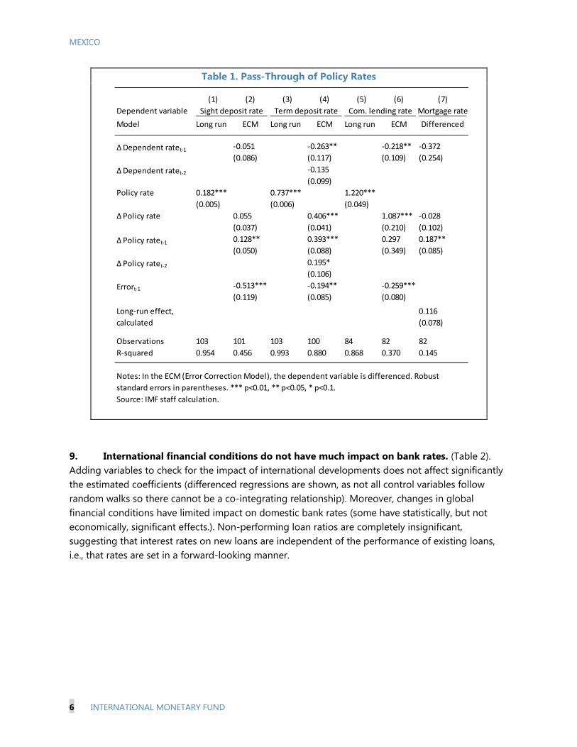
7. The transmission of the policy rate to market rates is statistically significant in all cases, except for mortgage rates (Table 1). For sight deposits, pass-through is low, with a one percentage point increase in the policy rate leading to a 0.2 percentage point rise in the deposit rate. For term deposits the pass-through is stronger, but remains below unity at 0.7. For commercial lending rates, however, pass-through exceeds unity at 1.2. These results are broadly in line with findings from other countries, which have also failed to find a strong relationship with mortgages (e.g., Hofmann and Mizen (2004), Pedersen (2016), and the studies cited in De Bondt (2005)), but found strong pass-through to corporate loans, occasionally exceeding unity (studies cited in De Bondt (2005)). The low pass-through to sight deposits, however, appears to be more unusual, at least compared to findings from Europe, which report full pass-through in the long term.

8. The pass-through to both lending and deposit rates is very rapid. The dynamic specifications show that pass-through is significant in either the current or the following month, and the long-run impact is achieved around the second month. The speed of adjustment varies from 0.2 to 0.5 of the deviation from the long-term relationship.

MEXICO


Table 1. Pass-Through of Policy Rates

9. International financial conditions do not have much impact on bank rates. (Table 2). Adding variables to check for the impact of international developments does not affect significantly the estimated coefficients (differenced regressions are shown, as not all control variables follow random walks so there cannot be a co-integrating relationship). Moreover, changes in global financial conditions have limited impact on domestic bank rates (some have statistically, but not economically, significant effects.). Non-performing loan ratios are completely insignificant, suggesting that interest rates on new loans are independent of the performance of existing loans, i.e., that rates are set in a forward-looking manner.

(1) (2) (3) (4) (5) (6) (7)

Dependent variable

Model Long run Long run Long run

-0.051 -0.263** -0.218** -0.372

(0.086) (0.117) (0.109) (0.254)

-0.135

(0.099)

0.182*** 0.737*** 1.220***

(0.005) (0.006) (0.049)

0.055 0.406*** 1.087*** -0.028

(0.037) (0.041) (0.210) (0.102)

0.128** 0.393*** 0.297 0.187**

(0.050) (0.088) (0.349) (0.085)

0.195*

(0.106)

-0.513*** -0.194** -0.259***

(0.119) (0.085) (0.080)

0.116

(0.078)

Observations 103 101 103 100 84 82 82

R-squared 0.954 0.456 0.993 0.880 0.868 0.370 0.145

Source: IMF staff calculation.

Sight deposit rate Term deposit rate Com. lending rate Mortgage rate

ECM ECM ECM Differenced

Errort-1

Long-run effect,

calculated

Notes: In the ECM (Error Correction Model), the dependent variable is differenced. Robust

standard errors in parentheses. *** p<0.01, ** p<0.05, * p<0.1.

Δ Dependent ratet-1

Δ Dependent ratet-2

Policy rate

Δ Policy rate

Δ Policy ratet-1

Δ Policy ratet-2

MEXICO


Table 2. Pass-Through of Policy rates with Controls

10. In summary, monetary policy appears to be an effective tool in shaping bank rates in Mexico, as the transmission of policy rates to corporate lending rates is found to be rapid and strong. The detailed results contain some further interesting findings:

Pass-through to commercial lending rates is particularly strong and the coefficient exceeds one. This could be explained by banks raising lending rates by more than their cost of funds, because higher rates increase the risk of default of their clients, everything else equal.3

Pass-through to deposit rates is lower, and especially low for sight deposits, but still statistically significant. The finding of a partial pass-through to deposits and more than full pass-through to commercial lending rates suggests that bank margins tend to increase when the interest rate increases.

The absence of a statistically significant impact on mortgage rates can be attributed to two factors. First, the prevalence of fixed rate mortgages naturally reduces the responsiveness to a short-term policy instrument. Long rates have been coming down in recent years, which could explain the downward trend. Second, recent financial reforms have made the mortgage market more competitive.

3 De Bondt (2005) lists pass-through coefficients above 1 from studies on various European countries, especially for loans to firms. He argues that this suggests the absence of credit rationing, because banks are lending at the margin to borrowers whose risk is affected by small increases in interest rates. If banks rationed credit to the safest borrowers only, this would not occur.

Dependent variable

Δ Sight

deposit

rate

Δ Term

deposit

rate

Δ Com.

lending

rate

Δ

Mortgage

rate

Δ Policy rate 0.150*** 0.680*** 1.134*** 0.080

(0.033) (0.065) (0.282) (0.115)

Δ NPL 0.130 -0.009

(0.165) (0.101)

Δ VIX -0.004* 0.001 -0.004 -0.012

(0.002) (0.002) (0.008) (0.009)

Δ EMBI 0.001* 0.000 0.004* 0.001

(0.000) (0.000) (0.002) (0.001)

Observations 101 101 83 83

R-squared 0.193 0.782 0.268 0.050

Robust standard errors in parentheses

*** p<0.01, ** p<0.05, * p<0.1

MEXICO


References

De Bondt, Gabe, 2005, “Interest Rate Pass-Through: Empirical Results for the Euro Area,” German Economic Review, Vol. 6(1), pp. 37-78.

Grigoli, Francesco and Jose Mota, 2015, “Interest Rate Pass-through in the Dominican Republic,” IMF Working Papers, No. 15/260.

Hofmann, Boris and Paul Mizen, 2004, “Interest Rate Pass-through and Monetary Transmission: Evidence from Individual Financial Institutions’ Retail Rates,” Economica, Vol 71(281). Pp. 99-123.

Mishkin, Frederic, 1996, “The Channels of Monetary Transmission: Lessons for Monetary Policy,” NBER Working Papers, No. 5464.

Pedersen, Michael, 2016, “Pass-through, expectations, and Risks. What Affects Chilean Banks’ Interest Rates?” Banco de Chile Working Papers, No. 780.

Sidaoui, Jose and Manuel Ramos-Francia, 2008, “The Monetary Transmission Mechanism in Mexico: Recent Developments,” BIS Papers, No. 35, pp. 363-94.

MEXICO


GLOBAL CONDITIONS AND CAPITAL FLOWS TO EMERGING MARKETS: HOW SENSITIVE IS MEXICO?1 The open capital account and large foreign holdings of Mexican assets naturally expose Mexico to changes in global conditions, such as an abrupt shift in investor sentiment toward emerging markets. Using a panel of gross capital flows to 30 emerging markets, this paper evaluates the sensitivity of Mexico’s foreign funding to global shocks between 2001 and 2015 and compares it to other emerging markets (EMs), in particular in Latin America. We find that global factors, such as changes in risk aversion or commodity prices, affect Mexico’s capital account mostly through their effect on the bond market. Between 2010 and 2015, half of the variance in Mexico’s bond inflows was explained by changes in global conditions. When compared to other EMs, Mexico’s bond market is among the most sensitive. A. Introduction

1. The last decade has re-emphasized the importance of common factors in driving capital flows, in particular to emerging markets. A number of recent papers have documented how global conditions can drive capital flows by non-residents to EMs, even more so than for advanced countries (e.g., Forbes and Warnock, 2012; Fratzscher, 2012). In the last few years, unconventional monetary policy by several advanced countries has been found to drive some of bond and equity inflows to EMs (e.g., Fratzscher, Lo Duca, and Straub, 2013). Although the specific “push” factors and their importance vary across studies, a consensus has emerged on the role of U.S. monetary policy, the supply of global liquidity (especially in US dollars), and global risk aversion in helping explain the high synchronicity of capital flows to EMs (Milesi-Ferretti and Tille, 2011, Shin, 2012, Rey, 2013, Ahmed and Zlate, 2014, among others).

2. Portfolio and bank related flows, which account for most of the foreign funding received by Mexico over the past few years, are more synchronized than other flows. Portfolio equity and bond flows to Mexico have increased significantly since 2010. The stock of foreign portfolio investment in Mexico has reached US$456 billion (40 percent of GDP) at end-2015 (see below). Contrary to FDI flows however, which follow mainly idiosyncratic dynamics, portfolio and bank related flows can co-move strongly across EMs as a

1 Prepared by Damien Puy

MEXICO


result of “push” factors, even in the absence of common fundamentals across recipient markets (Puy, 2015 and Figure).

B. Empirical methodology

3. This paper evaluates the sensitivity of Mexico’s capital inflows to global conditions and compares it to other EMs, in particular in Latin America. Building on Cerutti and others (2015), we first extract common factors in gross inflows to EMs - distinguishing between Portfolio Equity flows, Portfolio Bonds flows, and Other Investment (OI) to Banks – and study how different EMs react to deviations in the estimated (asset-specific) common factors.2 We focus on quarterly capital inflows during the period 2001Q1-2015Q1 for a set of 30 EMs. All series are measured in US dollars, divided by the recipient country GDP (also measured in US dollars) and normalized.

4. In practice, the following latent factor model is estimated for each type of gross capital inflow:

, , (1)

where , is the (normalized) inflow of a specific type to country i in quarter t, is the (unobserved) factor affecting all EMs in our sample at time t, is the (unobserved) regional factor affecting all countries belonging to region j at time t, and and designate country-specific factor loadings measuring the responses of country i to the common EM and regional factors respectively. Finally, , is an unobserved country-specific residual. Given that the factors are unobservable, standard regression methods do not allow for estimation of the model. We rely on Bayesian techniques as in Kose, Otrok and Whiteman (2003) for the estimation.3

5. After estimating the common EM factors driving flows, we measure their influence on the different countries. The cross-country heterogeneity is summarized in the factor loadings and the variance decomposition , which is computed as follows:

/ , (2)

Intuitively, measures the instantaneous impact on country i of a sudden change in the common EM factor . The variance decomposition estimates the share of the total variance of country i’s funding that can be attributed to the common EM dynamics over the sample period. Both statistics are reported and discussed below.

2 Consistent with the residence criterion of balance-of-payments statistics, the term capital gross “inflows” refers to changes in the financial liabilities of a domestic country vis-à-vis non-residents. Resident outflows are not analyzed as we are interested in the factors driving international investors’ behavior vis-à-vis recipient EMs. We focus on portfolio flows and bank flows only, since FDI and OI- to non-banks do not co-move across EMs (see Cerutti et. al. (2015) for a discussion). The breakdown of Other Investments into banks and non-banks follows Milesi-Ferretti and Tille (2011), where OI to Banks captures those OI transactions or holdings with banks as the domestic counterpart. 3 See Cerutti et. al. (2015) and references therein for a full description of the estimation methodology.

MEXICO


C. Key Findings

6. Gross capital inflows to EMs co-move considerably, mainly as a result of global “push” factors. Common factors are precisely extracted from both bank-related and portfolio inflows, suggesting that gross inflows co-move substantially across EMs, although the dynamics of inflows can sometimes diverge across types of asset (equity, bond or bank flows). Sudden negative changes in the factors correlate well with known stress events in advanced economies and major monetary policy change in core countries, whereas positive changes indicate an improvement in global conditions.4

7. Global conditions affect Mexico’s capital account mostly through the bond market. Over the full sample (2001Q1-2015Q4), more than 30 percent of the variance in Mexico’s external bond funding was driven by the common EM bond factor. In contrast, foreign equity and bank flows entering Mexico were marginally driven by their respective common EM dynamics. This suggests that they follow more closely changes in local or regional – rather than global – conditions.

8. Global conditions have affected bond flows to Mexico more strongly since 2010, which coincides with the introduction of Mexico in the WGBI. Contrasting the full sample with sub-sample analysis reveals an increase in the sensitivity of Mexico’s bond inflows to global conditions. Between 2010 and 2015, almost half of the variance in Mexico’s bond funding can be explained by the common EM dynamic, compared to only 30 percent before 2010. This is the highest among all EMs over that period.

4 The drivers behind the estimated common factors are discussed in more detail next section. For a full discussion, see Cerutti et. al. (2015).

MEXICO


9. Sudden changes in global conditions affect Mexico’s bond market more than other countries in Latin America. We compare the coefficients estimated using bond inflows for all countries between 2010 and 2015. The estimated beta for Mexico is around 0.4, implying that a unit standard deviation in the common EM factor will generate, on impact, a 0.4 standard deviation in bond flows to Mexico. Although Mexico’s response is the highest among Latin American countries, it is still smaller than other major EM bond markets, such as Turkey or South Africa.

MEXICO


D. What drives the common dynamics in bond flows?

10. Changes in risk aversion, oil prices or growth in key EMs are particularly important in explaining global bond flows. Regressing the estimated EM bond factor reveals that global risk aversion (measured by the VIX), oil prices and growth in both advanced and emerging markets affect the common EM bond dynamic, with the expected sign (see Appendix). The explanatory power of the VIX and oil prices, in particular, are strong. Still, using only the VIX and oil prices would fail to capture all changes in the direction of the factor. In fact, using all the traditional variables used in most empirical contributions as proxies for global push factors would still capture only a fraction of the variance explained by the estimated factor.5 This in turn tends to support the latent factor approach.

E. Why is Mexico so sensitive?

11. Large foreign holdings of domestic assets naturally expose Mexico to foreign shocks. Portfolio flows to Mexico have increased significantly since Mexico’s inclusion in the WGBI in 2010. The stock of foreign portfolio investment in Mexico reached US$456 billion (40 percent of GDP) at end-2015. Foreigners now hold 35 percent of local-currency government bonds, among the highest among EMs (see below). Although this strong presence of foreign investors in Mexico reflects their confidence in the economic policy framework and the depth and liquidity of its foreign exchange and bond markets, it exposes Mexico to shocks originating abroad, such as shifts in investor sentiment toward EMs.

12. The presence of international mutual funds in Mexico’s bond market might also contribute to increase Mexico’s sensitivity to push factors. Some foreign non-bank investors, such as international mutual funds, have been found to transmit shocks in advanced countries to a wide range of markets and often independently of the state of local fundamentals ((Raddatz and Schmukler (2012), Jotikasthira et al. (2012), Puy (2015)). Cerutti et al. (2015) recently confirmed this

5 See Cerutti et. al. (2015) for a full discussion of that point.

MEXICO


finding and found that countries relying more on international funds (e.g., mutual funds, ETFs) among their non-resident investors are significantly more sensitive to global push factors. The growing presence of international funds in Mexico’s foreign investor base, in particular cross-over funds, since 2010 might generate stronger sensitivity (see below, lower right panel).6

F. Conclusion and Policy Implications

13. Our findings suggest that changes in external conditions have had a significant impact on bond inflows to Mexico, in particular since 2010. Going forward, sudden changes in market sentiment towards EM, shifts in commodity prices and or growth reversals in key EMs are likely to affect Mexico’s gross bond flows. The introduction of Mexico in the WGBI, in particular, has significantly increased the sensitivity of Mexico’s bond inflows to global conditions. Maintaining strong fundamentals should help in containing the size of a potential reversal of capital flows.

6 We define cross-over funds as funds investing globally or to a wide range of EMs (as opposed to funds dedicated to Mexico).

MEXICO


Figure 1. Portfolio Liabilities in Mexico and Foreign Investor Base

Sources: National authorities; Haver; EPFR; Bloomberg; and IMF staff calculations.

5

10

15

20

25

30

35

40

45

2005 2006 2007 2008 2009 2010 2011 2012 2013 2014 2015

d) Mutual Fund Holdings in Mexico - by Fund Geographic Focus(USD, billions)

Other

Mexico

Latam

Global-EM

Global

-10

-5

0

5

10

15

20

25

30

2007 2008 2009 2010 2011 2012 2013 2014 2015 2016

Equity

Bonds

Total

a) Gross Portfolio Inflows(USD, billions)

0

5

10

15

20

25

30

35

40

45

2002 2003 2004 2005 2006 2007 2008 2009 2010 2011 2012 2013 2014 2015

Equity Public debt, MXN Public debt, FX Private debt

b) Mexico: Foreign-Held Portfolio Liabilities(In percent of GDP)

0

5

10

15

20

25

30

35

40

45

0

2

4

6

8

10

12

14

2008 2009 2010 2011 2012 2013 2014 2015 2016

Short-term (CETES)

Long-term

Foreign Holdings,percent of totaldebt (RHS)

c) Non-Residents' Holdings of Local Sovereign Debt(In percent of GDP: as of September 2016)

MEXICO


References

Ahmed, Shaghil, and Andrei Zlate, 2014, “Capital flows to emerging markets: A brave new world?” Journal of International Money and Finance, Vol. 48, pp. 221-248.

Cerutti, Eugenio, Stijn Claessens, and Damien Puy, 2015, “Push factors and capital flows to EMs: why knowing your lender matters more than fundamentals?” IMF Working Paper, 2015/127.

Forbes, Kristin J., and Francis E. Warnock, 2012, “Capital flow waves: Surges, stops, flight, and retrenchment” Journal of International Economics, Vol. 88, N0. 2, pp. 235-251

Fratzscher, Marcel, 2012, “Capital flows, Push versus pull factors and the global financial crisis,” Journal of International Economics, Vol. 88, No. 2, pp. 341-356.

Fratzscher, Marcel, Marco Lo Duca, and Roland Straub, 2013, “On the International Spillovers of U.S. Quantitative Easing,” Discussion Papers of DIW Berlin 1304, DIW Berlin, German Institute for Economic Research.

IMF, 2013, “The Yin and Yang of Capital Flow Management: Balancing Capital Inflows with Capital Outflows,” by Jaromir Benes, Jaime Guajardo, Damiano Sandri, and John Simon, World Economic Outlook, Chapter 4, Fall.

Jotikasthira, Chotibhak, Christian Lundblad, and Tarun Ramadorai, 2012, “Asset Fire Sales and Purchases and the International Transmission of Funding Shocks,” Journal of Finance, Vol. 67, No. 6, pp. 2015–050.

Kose, Ayhan, Christopher Otrok, and Charles H. Whiteman, 2003, “International Business Cycles: World, Region, and Country-Specific Factors,” American Economic Review, Vol. 93, No. 4, pp. 1216-239.

Milesi-Ferretti, Gian Maria, and Cédric Tille, 2011, “The Great Retrenchment: International Capital Flows during the Global Financial Crisis,” Economic Policy, Vol. 26. No. 66, pp. 285-342.

Puy, Damien, 2015, “Mutual Fund Flows and the Geography of Contagion,” Journal of International Money and Finance.

Raddatz, Claudio, and Sergio Schmukler, L., 2012, “On the International Transmission of Shocks: Micro-evidence from Mutual Fund Portfolios,” Journal of International Economics, Vol. 88, No. 2, pp. 357-74.

Rey, Hélène, 2013, “Dilemma not Trilemma: The Global Financial Cycle and Monetary Policy Independence,” in Proceedings of the 2013 Federal Reserve Bank of Kansas City Economic Symposium at Jackson Hole, pp. 285-333.

Shin, Hyun Song, 2012, “Global Banking Glut and Loan Risk Premium” Mundell-Fleming Lecture, IMF Economic Review Vol. 60, No. 2, pp. 155-92.

MEXICO


Appendix I. Sample of Countries

Sample of Countries

Latin America Asia Emerging Europe Other

Argentina India Belarus Turkey

Brazil China, Mainland Kazakhstan South Africa

Chile Indonesia Bulgaria Israel

Colombia Republic of Korea Russian Federation

Mexico Malaysia Ukraine

Peru Pakistan Czech Republic

Uruguay Philippines Slovak Republic

Venezuela, Rep. Bol. Thailand Estonia

Latvia

Hungary

Lithuania

Croatia

Slovenia

Poland

Romania

MEXICO


Appendix II. Regression Results – EM Bond Factor

(1) (2)

Full Sample Post crisis

vix -0.0465*** -0.0635***

(0.0122) (0.0116)

wti 0.0106*** 0.00836*

(0.00255) (0.00457)

L.adv_growth -0.0708* -0.0616

(0.0393) (0.0861)

L.bric_growth 0.0712*** 0.339***

(0.0259) (0.0545)

fed funds 0.241 -1.985

(0.195) (4.319)

_cons -0.113 -1.040**

(0.350) (0.391)

N 59 24

R-sq 0.519 0.749

MEXICO


WELFARE GAINS FROM HEDGING OIL-PRICE RISK1 Since at least 2001, Mexico’s federal government has hedged the near-term fiscal impact of declines in oil prices through put options. Using a structural model calibrated to the Mexican economy, we quantify the overall benefits of this long-standing policy. Compared to a self-insurance alternative, we find welfare gains from hedging through put options equivalent to a permanent increase in consumption of 0.4 percent. These gains arise mostly from a reduction in sovereign spreads and to a lesser extent from smoothing income volatility. In terms of design, expanding the program to cover domestic fuel sales could yield further gains once gasoline and diesel markets are liberalized. Relying more on liquid instruments—such as options on the Brent—is an avenue worth exploring to ensure the program remains cost effective.

A. Introduction

1. Mexico’s hedging program has the objective to hedge the value of Mexican oil exports at a strike price that is consistent with the one assumed in the budget for each year. To meet this objective, the program involves buying Asian put options to insure the price of oil for the whole year. 2 The execution involves purchasing options with Maya oil—a type of Mexican heavy crude oil—and Brent as underlying assets, although the former dominates as Maya oil represents about 80 percent of Mexico’s oil export volumes.

2. The program helped cushion the fiscal impact of the decline in oil prices in 2009, 2015, and it is expected to do so again this year. Since 2001, the options had a cost, on average, of 0.1 percent of GDP per year, but were exercised only in 2009 and 2015, yielding payoffs close to 0.6 percent of GDP in each occasion. It is expected that the options will be exercised again this year, yielding estimated revenues for 0.3 percent of GDP.

1 Prepared by Chang Ma and Fabian Valencia. The authors thank Dora Iakova, Alexander Klemm, Damien Puy, Robert Rennhack, Alejandro Werner, seminar participants at the IMF and the Bank of Mexico for comments and suggestions. 2 An American or European put option is exercised if the spot price on a particular day exceeds the strike price. In contrast, an Asian put option is exercised if the average spot price for a pre-determined period, which in the case of Mexico is one year, exceeds the strike price. In this way, Mexico guarantees a minimum average price of oil for the whole fiscal year.

-

0.1

0.2

0.3

0.4

0.5

0.6

0.7

2001

2002

2003

2004

2005

2006

2007

2008

2009

2010

2011

2012

2013

2014

2015

2016

Cash Flow from Options(In percent of GDP)

Inflows

Outflows

Source: National authorities; and IMF staff calculations.

MEXICO


3. This paper examines the welfare gains for Mexico from having the hedging program. Using a structural model, this paper asks three questions: 1) how large are the welfare gains from using put options to hedge oil price risk; 2) what are the main channels through which these gains operate; and 3) what design considerations can increase the benefits of the program further.

B. Model Setup

4. The model summarizes a small open economy with representative consumers who receive income from oil and non-oil sources and consume a tradable good. The model is a standard sovereign default model (Arellano, 2008). It is assumed that a social planner (i.e. the government) makes decisions aimed at maximizing the present discounted value of private agents’ utility derived from consumption ( tC ):

00

( )tt

t

E U C

.

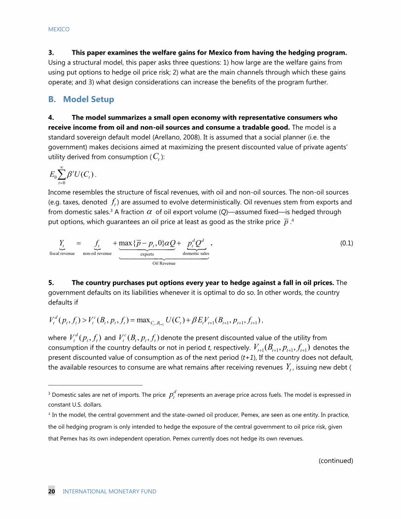
Income resembles the structure of fiscal revenues, with oil and non-oil sources. The non-oil sources (e.g. taxes, denoted tf ) are assumed to evolve deterministically. Oil revenues stem from exports and from domestic sales.3 A fraction of oil export volume (Q)—assumed fixed—is hedged through put options, which guarantees an oil price at least as good as the strike price p .4

fiscal revenue non-oil revenue domestic salesexports

Oil Revenue

max{ ,0} d dt t t tY f p p Q p Q

. (0.1)

5. The country purchases put options every year to hedge against a fall in oil prices. The government defaults on its liabilities whenever it is optimal to do so. In other words, the country defaults if

1, 1 1 1 1(( , ) ( , , ) max ( , ,) )t t

d ct t t t t t t C B t t t t ttV p f V B p f EV BU C p f

,

where ( , )dt t tV p f and ( , , )c

t t t tV B p f denote the present discounted value of the utility from consumption if the country defaults or not in period t, respectively. 1 1 1 1( , , )t t t tV B p f denotes the present discounted value of consumption as of the next period (t+1), If the country does not default, the available resources to consume are what remains after receiving revenues tY , issuing new debt (

3 Domestic sales are net of imports. The price d

tp represents an average price across fuels. The model is expressed in

constant U.S. dollars. 4 In the model, the central government and the state-owned oil producer, Pemex, are seen as one entity. In practice,

the oil hedging program is only intended to hedge the exposure of the central government to oil price risk, given

that Pemex has its own independent operation. Pemex currently does not hedge its own revenues.

(continued)

MEXICO


1tB ) at price tq , repaying existing debt, tB , and purchasing put options to insure Q barrels of oil at a cost of ( )tp per barrel:

1 ( )t t t t t tC Y B q B Q p . (0.2)

If the country defaults, it resorts to autarky but it can still hedge oil price risk.5 In addition to being unable to issue debt, default implies an income loss equal to h.6 In case of default, the resource constraint boils down to

( )t t t tY hC Q p . (0.3)

There is, however, a positive probability ( ) that the country exits its default status and issues debt again. This possibility is taken into account in the calculation of the present discounted value of future utility of consumption and hence in the default decision:

1 1 1 1( , ) (0, , )( ) ) (1 ( , )d dt t t t t t t tt t t tV p f E V p f E V p fU C

6. The price of sovereign bonds and put options is determined in international financial markets by risk neutral investors. The underlying assumption is that international investors hold diversified portfolios and price bonds and options as to ensure an expected return equal to the international risk-free rate ( *r ). Because the ex-ante rate of return on these instruments is the same, the risk-neutral investor is indifferent between holding a bond or being the counterpart of a put option.

1 1 11 *

1 ( , , )( , , )

1t t t t

t t t t

E D B p fq B p f

r

, with 1 1 1( , , ) 1t t tD B p f if country defaults (0.4)

1*

[max{ ,0}]( )

1t t

t

E p pp

r

(0.5)

7. The model is calibrated to the Mexican economy taking some parameters directly from data and the literature, while estimating others to match chosen data moments. The full model and solution are described in Appendix A. We take from the literature the coefficient of risk aversion. We measure directly in the data the real risk-free interest rate (approximated by the yield on 1-year U.S. treasury bonds deflated with the U.S. GDP deflator); the oil-price process (estimated using an AR1 on the price of the Mexican mix); oil export and domestic sales (net of imports) volumes; the fraction of export volumes hedged; and the deterministic growth rate of non-oil

5 The underlying assumption is that debt and financial derivatives are separate markets.

6 Following Arellano (2008), we assume that income is lower than under no default but it can at most drop to some

value *y , which will be calibrated to match sovereign spreads in the data.

MEXICO


revenues. The discount factor and the parameter *y of the loss function under default are chosen as to match the government’s gross financing needs and the average Mexican sovereign spread over U.S. treasury bonds. Tables B1-B3 in the appendix show the complete set of parameter values and simulated data moments.

C. Welfare gains and channels

8. The benefits of hedging are computed relative to a self-insurance alternative. Using Monte Carlo simulations, we construct paths for consumption and contrast them with those from a version of the model without hedging.7 In absence of hedging, consumption-smoothing takes place solely through issuing debt. The welfare gains from hedging can be expressed in terms of the permanent increase in consumption that would yield the same present discounted value as in the model with hedging.

9. The estimated welfare gains are equivalent to a 0.4 percent permanent increase in consumption and stem mostly from a reduction in sovereign spreads. These gains are smaller than those reported in Boreinsztein and others (2013)8 but are within the range of estimates found in the literature from issuing catastrophic bonds (0.12 percent, Borensztein and others, 2016) and GDP-indexed bonds (0.46 percent, Hatchondo and Martinez, 2012), which are alternatives to insure against downside risks. 9 Hedging is beneficial in the model because of two channels at work: a reduction in income volatility and a reduction in borrowing spreads. Both are the consequence of lower downside risks from oil-price fluctuations. We decompose the overall welfare gains into these two channels to conclude that about 90 percent of the gains are explained by a reduction in borrowing costs.10 Sovereign spreads are 30 basis points lower, on average, in the model with hedging than in the model with no hedging.

7 The simulation is implemented by initializing the system at some random initial level of debt, 0B , while oil prices are initialized at their unconditional mean. Using the optimal solutions, we simulate 500 paths of 2,000 periods each, for which we compute the average present discounted value of consumption after dropping the initial 500 periods.

8 Boreinsztein and others (2013) report welfare gains from hedging though options (at a one-year horizon) of about 1-percent permanent increase in consumption. In their model, there is no default, while in principle, the option of default can be seen as an insurance mechanism in case of a very negative shock. 9 Lopez-Martin and others (2016) conduct a similar analysis than ours in a sovereign default model in which public and private sector decisions are modeled separately. While they do not directly compute welfare gains, they show that the public sector is willing to pay an important fraction of commodity revenues for options as insurance against declines in oil prices.

10 The decomposition is implemented by solving the model with no hedging using the bond pricing function from the model with hedging. This implies that any remaining welfare gains in this model would be attributed to the income volatility channel.

MEXICO


D. Design Considerations

10. Sensitivity analysis on the model offers insights for the design of the hedging program. The design of the program requires making decisions on the number of barrels hedged, the strike price, the underlying asset, and the instrument to be used, which ultimately affect the cost of the options. By looking at how the welfare gains change when key parameters of the model are modified we can offer some insights about some of these design questions. In particular, we focus on the size of the program (or volume hedged), the strike price, and the cost of the options.11

Size of the Program

11. The welfare gains increase with the number of barrels hedged. On average, Mexico hedged a range between 210 and 230 million barrels a year during 2010-2015,12 reflecting approximately the volume difference between exports and imports, and representing on average about half of export volumes. For 2017, Mexico increased the volume hedged to 250 million barrels (from 212 million in 2016). The model suggests that it is welfare-enhancing to increase the number of barrels hedged (simulated by varying the parameter ). Welfare gains peak only after an implausibly large program (9 times exports).

Welfare Gains and Volume Hedged

11 Instrument considerations involve first deciding whether buying put options or selling forward are preferable. Boreinsztein and others (2013) show that for hedging horizons of up to 5 years, the welfare gains from selling forward or buying put options are comparable. The choice for Asian options serves the purpose of hedging the average price of oil for the fiscal year in question (see Duclaud and Garcia, 2012 for a description of the Mexican hedging program). 12 The Cuenta publica reports by the Auditoria Superior Federal (Federal Audit Office) provide the cost and volume hedged for each year since 2006.

0

200

400

600

800

1000

1200

1400

1600

1995

1996

1997

1998

1999

2000

2001

2002

2003

2004

2005

2006

2007

2008

2009

2010

2011

2012

2013

2014

2015

a) Oil Production(Millions of barrels)

Production Exports

Imports Domestic Consumption

Source: National authorities; and IMF staff calculations.

0

2

4

6

8

10

12

14

16

- 222 444 667 889 1,111 1,333 1,556 1,778 2,000

Percent of Export Volumes

b) Welfare Gains and Volume Hedged(In percent of consumption)

MEXICO


12. A larger hedging program can also help reduce volatility of domestic oil revenues once gasoline and diesel markets are fully liberalized. Mexico exports about half of its oil production, while the other half is refined and sold domestically—together with imported oil derivatives—at regulated prices.13 Mexico is gradually liberalizing domestic fuel markets and the process is expected to be completed by 2018. Expanding the hedging program to cover domestic sales, which could be implemented by having Pemex develop its own hedging program, can help smooth the resulting volatility in overall fiscal revenues.

Strike Price

13. The choice for strike price in Mexico has been close to optimal. The choice for the strike price in Mexico is informed by estimates of the long-run price of oil derived from a formula spelled out in the 2006 Fiscal Responsibility Law, which corresponds to a weighted average between historical and futures prices. In the model, this long-run price is the unconditional mean of the estimated AR1 oil-price process. The baseline calibration uses a strike price close to 0.9 times the unconditional mean, which approximates the strike price chosen by Mexico in past years.14 The simulations show that welfare gains peak when the strike price is about equal to the unconditional mean. In practice, this suggests that the choice for strike price in Mexico has been close to optimal.

Welfare Gains and Strike Price

Source: National authorities and staff estimates. Note: 1/ The long-run oil price is estimated computing the unconditional mean from an AR1 process estimated for each year. The average

ratio of the actual strike price to this estimate of the long-run oil price is 0.86. Since in the model the oil price process is time-invariant, we use this ratio to calibrate the strike price. The right figure shows the resulting welfare gains for various strike prices, expressed as a ratio to the unconditional mean, including for the baseline value of 0.86.

13 Pemex is exposed to oil-price risk on both foreign and domestic sales as it receives international prices on the latter. However, additional revenues for the federal government from a wider difference between domestic and international prices partly offset the fiscal impact of oil-price declines. Starting in 2016, fuel excises were fixed at levels close to optimal (IMF 2015) while domestic prices were allowed to move closer in line with international prices. The 2017 economic package envisages liberalizing some markets one-year ahead of schedule with the intention to have fully market-determined prices by 2018. 14 We estimate the AR1 process for oil in 1-year rolling windows. For each year we compute the ratio of the actual strike price (taken from the data) to the unconditional mean from the oil process estimated for that year. The average of this ratio is 0.86, which is used in the baseline model. The calculation also approximates well the moneyness of the options, calculated as the ratio of the strike price to the average futures price for the subsequent year.

0

20

40

60

80

100

120

2007 2008 2009 2010 2011 2012 2013 2014 2015 2016

a) Actual Strike Price and Long-run Oil Price 1/(In USD per barrel)

Actual Strike Price Long-run Oil Prices

0

0.1

0.2

0.3

0.4

0.5

0.6

0.7

0.7 0.8 0.9 1.0 1.1 2.0

Strike price as a ratio to unconditional mean of oil prices

b) Welfare Gains and Strike Price(In percent of consumption)

Baseline

MEXICO


Cost of Options and Base Risk

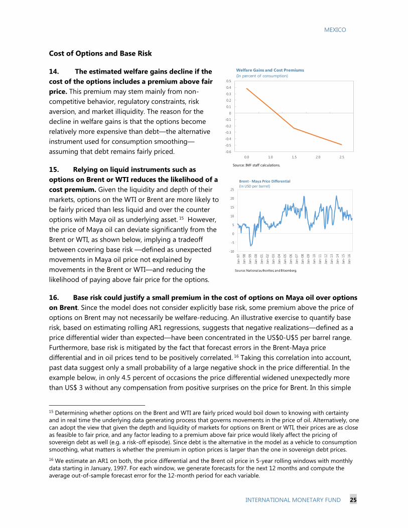
14. The estimated welfare gains decline if the cost of the options includes a premium above fair price. This premium may stem mainly from non-competitive behavior, regulatory constraints, risk aversion, and market illiquidity. The reason for the decline in welfare gains is that the options become relatively more expensive than debt—the alternative instrument used for consumption smoothing—assuming that debt remains fairly priced.

15. Relying on liquid instruments such as options on Brent or WTI reduces the likelihood of a cost premium. Given the liquidity and depth of their markets, options on the WTI or Brent are more likely to be fairly priced than less liquid and over the counter options with Maya oil as underlying asset. 15 However, the price of Maya oil can deviate significantly from the Brent or WTI, as shown below, implying a tradeoff between covering base risk —defined as unexpected movements in Maya oil price not explained by movements in the Brent or WTI—and reducing the likelihood of paying above fair price for the options.

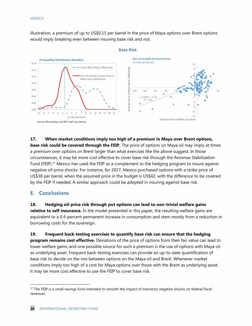
16. Base risk could justify a small premium in the cost of options on Maya oil over options on Brent. Since the model does not consider explicitly base risk, some premium above the price of options on Brent may not necessarily be welfare-reducing. An illustrative exercise to quantify base risk, based on estimating rolling AR1 regressions, suggests that negative realizations—defined as a price differential wider than expected—have been concentrated in the US$0-U$5 per barrel range. Furthermore, base risk is mitigated by the fact that forecast errors in the Brent-Maya price differential and in oil prices tend to be positively correlated. 16 Taking this correlation into account, past data suggest only a small probability of a large negative shock in the price differential. In the example below, in only 4.5 percent of occasions the price differential widened unexpectedly more than US$ 3 without any compensation from positive surprises on the price for Brent. In this simple

15 Determining whether options on the Brent and WTI are fairly priced would boil down to knowing with certainty and in real time the underlying data generating process that governs movements in the price of oil. Alternatively, one can adopt the view that given the depth and liquidity of markets for options on Brent or WTI, their prices are as close as feasible to fair price, and any factor leading to a premium above fair price would likely affect the pricing of sovereign debt as well (e.g. a risk-off episode). Since debt is the alternative in the model as a vehicle to consumption smoothing, what matters is whether the premium in option prices is larger than the one in sovereign debt prices. 16 We estimate an AR1 on both, the price differential and the Brent oil price in 5-year rolling windows with monthly data starting in January, 1997. For each window, we generate forecasts for the next 12 months and compute the average out-of-sample forecast error for the 12-month period for each variable.

-10

-5

0

5

10

15

20

25

Jan-

97

Jan-

98

Jan-

99

Jan-

00

Jan-

01

Jan-

02

Jan-

03

Jan-

04

Jan-

05

Jan-

06

Jan-

07

Jan-

08

Jan-

09

Jan-

10

Jan-

11

Jan-

12

Jan-

13

Jan-

14

Jan-

15

Jan-

16

Brent - Maya Price Differential (In USD per barrel)

Source: National authorities; and Bloomberg.

-0.6

-0.5

-0.4

-0.3

-0.2

-0.1

0

0.1

0.2

0.3

0.4

0.5

0.0 1.0 1.5 2.0 2.5

Welfare Gains and Cost Premiums(In percent of consumption)

Source: IMF staff calculations.

MEXICO


illustration, a premium of up to US$0.15 per barrel in the price of Maya options over Brent options would imply breaking even between insuring base risk and not.

Base Risk

17. When market conditions imply too high of a premium in Maya over Brent options, base risk could be covered through the FEIP. The price of options on Maya oil may imply at times a premium over options on Brent larger than what exercises like the above suggest. In those circumstances, it may be more cost effective to cover base risk through the Revenue Stabilization Fund (FEIP).17 Mexico has used the FEIP as a complement to the hedging program to insure against negative oil-price shocks. For instance, for 2017, Mexico purchased options with a strike price of US$38 per barrel, when the assumed price in the budget is US$42, with the difference to be covered by the FEIP if needed. A similar approach could be adopted in insuring against base risk.

E. Conclusions

18. Hedging oil-price risk through put options can lead to non-trivial welfare gains relative to self-insurance. In the model presented in this paper, the resulting welfare gains are equivalent to a 0.4-percent permanent increase in consumption and stem mostly from a reduction in borrowing costs for the sovereign.

19. Frequent back-testing exercises to quantify base risk can ensure that the hedging program remains cost effective. Deviations of the price of options from their fair value can lead to lower welfare gains, and one possible source for such a premium is the use of options with Maya oil as underlying asset. Frequent back-testing exercises can provide an up-to-date quantification of base risk to decide on the mix between options on the Maya oil and Brent. Whenever market conditions imply too high of a cost for Maya options over those with the Brent as underlying asset, it may be more cost effective to use the FEIP to cover base risk.

17 The FEIP is a small savings fund intended to smooth the impact of transitory negative shocks on federal fiscal revenues.

0.00

0.02

0.04

0.06

0.08

0.10

0.12

0.14

-11 -9 -7 -5 -3 -1 1 3 5 7 9 11 13 15 17 19 21

In US$ per barrel

Probability Distribution Densities

Actual Brent-Maya differential

Out-of-sample forecast error inBrent-Maya differential

Source: Bloomberg; and IMF staff calculations.

y = 0.0814x + 1.153R² = 0.28

-12

-10

-8

-6

-4

-2

0

2

4

6

8

10

-120 -100 -80 -60 -40 -20 0 20 40

Fore

cast

err

or in

May

a-Br

ent

diffe

rent

ial

Forecast error in Brent oil prices

Out-of-sample Forecast Errors(In USD per barrel)

MEXICO


20. A larger program could be beneficial in the context of liberalized domestic fuel markets. So far, the exposure of consolidated public finances to oil-price volatility has stemmed from net exports. Once domestic fuel markets are liberalized, the larger exposure to oil-price volatility can be dealt with a larger hedging program, which could be implemented by having Pemex develop its own hedging program.

MEXICO


References

Arellano, Cristina, 2008. “Default risk and income fluctuations in emerging economies,” The American Economic Review, 2008, pp. 690–712.

Borensztein, Eduardo, Eduardo Cavallo, and Olivier Jeanne, 2015. “The Welfare Gains from Macro-Insurance Against Natural Disasters,” National Bureau of Economic Research WP#

Borensztein, Eduardo, Olivier Jeanne, and Damiano Sandri, 2013. “Macro-hedging for commodity exporters,” Journal of Development Economics, 2013, 101, 105–116.

Duclaud, Javier and Gerardo Garcia, 2012. “Mexico’s Oil Price–Hedging Program,” in Arezki, Rabah, Catherine Pattillo, Marc Quintyn, and Min Zhu (Editors), “Commodity Price Volatility and Inclusive Growth in Low-Income Countries.” International Monetary Fund, Washington D.C.

Hatchondo, Juan Carlos and Leonardo Martinez, 2012. “On the benefits of GDP-indexed government debt: lessons from a model of sovereign defaults,” Economic Quarterly, 98 (2), 139–158.

International Monetary Fund, 2015. “A Carbon Tax Proposal for Mexico,” Selected Issues Paper, Chapter 4.

Lopez-Martin, Bernabe, Julio Leal, and Andre Martinez Fritscher, 2016. “Commodity Price Risk Management and Fiscal Policy in a Sovereign Default Model,” Bank of Mexico manuscript.

Reinhart, Carmen, Kenneth Rogoff, and Miguel Savastano, 2003. “Debt Intolerance,” Brookings Papers on Economic Activity, 2003 (1), 1–74.

MEXICO


Appendix I. Model Structure

To simplify the solution of the model, all variables are first normalized by the non-oil income tf ,

which reduces the number of state variables to 2. The normalized problem, where small variables

denote normalized values (e.g. t

t

Ct fc ), is shown below:

Value function:

( , ) max ( , ), ( )c dt t t t tV b p V b p V p

Value function if there is no default:

1

11

, 1 1( , ) max ( , )1t t

c tt t c b t t t

cV b p G E V b p

1s.t. ( ) max{ - ,0}t t t t t t tc q Gb QG p y Q p p b

Value function under default 1

11 1( ) (0, ) (1 ) ( )

1d dt

t t t t t

cV p G E V p E V p

. . - ( ) - - ( )t t t t ts t c y QG p h y QG p

Price of sovereign bond and put options:

1 11 *

1 ( , )( , )

1t t t

t t

E D b pq b p

r

1*

[max{ ,0}]( )

1t t

t

E p pp

r

The model is solved through value function iteration using a pre-determined grid space for both

tb and tp . We start with an initial guess for bond prices ( , )iq b p for each bB and pP and

the value functions { ( , ), ( ), ( , )}d ci i iV b p V p V b p . In each iteration, we find the value for 1tb and

tc within the pre-determined grid that maximizes the value function. The value function and the

bond pricing equation are updated and used in the next iteration and so on. The procedure is

repeated until the value functions and the pricing equation converge (i.e. when the difference in

values between two iterations is small enough that some pre-determined convergence criteria).

MEXICO


MEXICO


Appendix II. Calibration

Table B. 1 – Parameter Values Parameters Value Source

Risk-free interest rate * 0.71%r U.S. Real Interest Rate (1-Year Treasury Bill): 1995-2015

Risk aversion 2 Standard Value in literature

Probability of redemption 0.11 Average years in default for Mexico: 1800-2010 (Reinhart, Rogoff, and Savastano, 2009)

Unconditional oil price p =48.84 Data

Oil price persistence =0.8403 Data

Oil price volatility =0.2869 Data

Export volume (normalized) 1/ Q =0.0047 Data

Domestic sales volume (normalized) 1/ dQ =0.0052 Data

Strike Price p = 0.86* [ ]tE p Data

Share of exports hedged =0.55 Data

Domestic oil price log 3.28 0.18logdt tp p Data

Growth rate of non-oil revenue G= 1.02 Data

Parameter to match moments

Discount rate =0.7182 Model simulation Output loss under default (threshold below which there is no loss)

*y =1.3302 Model simulation

1/ Corresponds to model normalized by non-oil income.

Table B.2 Simulated vs. Data Moments

Debt ratio 1/ Sovereign spreads

In percent

Model 51.76 3.51

Data 53.00 3.68 1/ The data counterpart to the debt ratio is the public sector’s gross financing requirements, expressed in percent of non-oil income.

Table B.3 Simulated Moments in Model with and without Hedging Debt ratio 1/ Sovereign spreads Default probability

In percent

Model with hedging 51.76 3.51 2.54

Model without hedging 49.98 3.82 2.70 1/ The data counterpart to the debt ratio is the public sector’s gross financing requirements, expressed in percent of non-oil income.

MEXICO


EVALUATING THE STANCE OF MONETARY POLICY1 Using an estimated Taylor rule and a small DSGE model, this study finds that the monetary policy stance in Mexico has shifted from accommodative to broadly neutral. A. Introduction

1. After a period of an unprecedentedly low policy rate, the monetary policy rate in Mexico was raised by a total of 175 basis points between December 2015 and September 2016. Following a 25 basis point increase in December 2015 (matching the U.S. rate move), interest rates were increased by 50 basis points each during an extraordinary session on February 17 and during regular monetary policy committee meetings on June 30 and September 29, 2016.

2. This paper provides an assessment of the monetary policy stance using various methods. A Taylor rule is used to compare the current policy rate to the rate implied by the estimated historical reaction function. In addition, a small open-economy DSGE model is used to estimate the neutral rate. The main conclusion is that the policy stance has shifted from an accommodative to broadly neutral or mildly restrictive.

B. Estimated Taylor Rule

3. A Taylor rule for Mexico is estimated using monthly data between 2006 and 2016. The results are presented in equation (1) below, where denotes the policy rate, ∗ measures deviations of inflation from the 3-percent permanent target, ∗ measures deviations of 12-months ahead inflation expectations from the target, ∗ is the deviation of output from potential, and to the current level of the Federal Funds Rate. The Federal Fund rate is added to the estimated reaction function since the Bank of Mexico frequently notes that it takes into account the relative monetary stance with the U.S. when setting the policy rate (Mexico and the U.S. have highly synchronized business cycles). It also serves as a proxy for the effect of global interest rates on Mexico’s interest rates. The estimation uses core inflation and one-year ahead expectations of core inflation taken from analysts’ surveys.

3.95 1.25 ∗ 0.13 ∗ 0.31 ∗ 0.30 (1)

4. The estimated Taylor rule captures well the behavior of the Bank of Mexico over the past ten years. An alternative version of the model, with the exchange rate added to equation (1) does not improve the fit further, which suggests that, historically, the Bank of Mexico has not responded to exchange rate changes beyond their impact on current and expected inflation. Changes in the Federal Funds rate explains only a small share of the variance in Mexico’s policy rate, and excluding it does not affect results significantly. Finally, adding a lagged dependent variable -

1 Prepared by Alexander Klemm and Damien Puy.

MEXICO


with an estimated coefficient of 0.88 - to allow for smoothness in policy rate changes, affects the predicted values and the dynamics of the estimated Taylor rule only marginally.

5. The cumulative increase in the policy rate over the past year has brought the policy rate slightly above the estimated historical reaction function. The tightening is consistent with Bank of Mexico’s message that they are tightening pre-emptively to guard against the risk of de-anchoring of inflation expectations in the context of a significant exchange rate depreciation over the past two and a half years.

C. The neutral interest rate

6. The empirical literature suggests that neutral interest rates in advanced economies have declined. Holston and others (2016) estimate neutral rates for the U.S., the euro area, Canada, and the United Kingdom and find a downward trend in neutral interest rates in all four economies. Moreover, they note a substantial co-movement across economies. Pescatori and Turunen (2015) estimate neutral policy rates for the United States, using a methodology that accounts for unconventional monetary policy measures. They also find a strong decline over time. Magud and Tsounta (2012) estimates of neutral interest rates in Latin America also establish a downward trend. The decline in global interest rates has been attributed to an increase in global saving rates related to demographic factors, increased demand for safe assets, low investment rates, and a decline in potential growth rates in a number of large economies. Since Mexico is a small open economy, the reduction in neutral rates in major trading partners is likely to be associated with a decline in Mexico’s neutral interest rate as well.

7. A small open-economy DSGE model is used to estimate the neutral interest rate for Mexico directly. The model consists of a standard IS curve, a Phillips curve, and a Taylor rule. It provides an estimate of the neutral rate, which in this model is the real rate that would prevail if inflation and output gaps were closed.

IS curve: 0.71 0.70 ∗ 0.00

(2)

where x is the output gap, π is the annualized quarterly (core) inflation rate, r* is the neutral real interest rate, and d is the rate of depreciation. Phillips curve:

0.48 0.55 0.33 (3)

Taylor rule: ∗ 0.19 3 0.17 (4)

1

2

3

4

5

6

7

8

9

10

Aug

-07

Jan-

08

Jun-

08

Nov

-08

Apr

-09

Sep-

09

Feb-

10

Jul-

10

Dec

-10

May

-11

Oct

-11

Mar

-12

Aug

-12

Jan-

13

Jun-

13

Nov

-13

Apr

-14

Sep-

14

Feb-

15

Jul-

15

Dec

-15

May

-16

Oct

-16

Taylor Rule vs Actual Policy Rate(In percent)

Actual

Taylor Rule

95% confidence interval

Source: IMF staff calculations

MEXICO


The depreciation of the exchange rate is modeled as an AR(1) process:

0.07 (5)

The neutral interest rate follows a simple process with persistent shocks z.2

∗ 2.72 (6)

. 99 (7)3

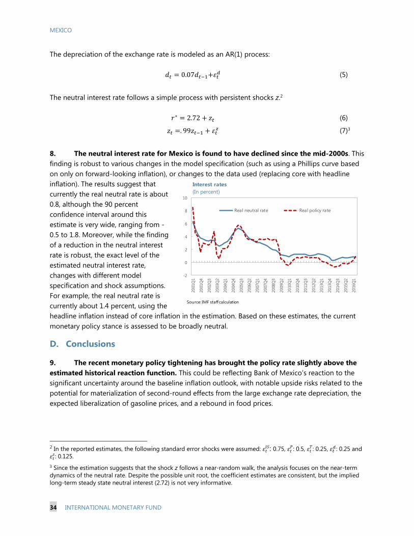
8. The neutral interest rate for Mexico is found to have declined since the mid-2000s. This finding is robust to various changes in the model specification (such as using a Phillips curve based on only on forward-looking inflation), or changes to the data used (replacing core with headline inflation). The results suggest that currently the real neutral rate is about 0.8, although the 90 percent confidence interval around this estimate is very wide, ranging from -0.5 to 1.8. Moreover, while the finding of a reduction in the neutral interest rate is robust, the exact level of the estimated neutral interest rate, changes with different model specification and shock assumptions. For example, the real neutral rate is currently about 1.4 percent, using the headline inflation instead of core inflation in the estimation. Based on these estimates, the current monetary policy stance is assessed to be broadly neutral.

D. Conclusions

9. The recent monetary policy tightening has brought the policy rate slightly above the estimated historical reaction function. This could be reflecting Bank of Mexico’s reaction to the significant uncertainty around the baseline inflation outlook, with notable upside risks related to the potential for materialization of second-round effects from the large exchange rate depreciation, the expected liberalization of gasoline prices, and a rebound in food prices.

2 In the reported estimates, the following standard error shocks were assumed: : 0.75, : 0.5, : 0.25, : 0.25 and

: 0.125. 3 Since the estimation suggests that the shock z follows a near-random walk, the analysis focuses on the near-term dynamics of the neutral rate. Despite the possible unit root, the coefficient estimates are consistent, but the implied long-term steady state neutral interest (2.72) is not very informative.

-2

0

2

4

6

8

1020

01Q

1

2001

Q4

2002

Q3

2003

Q2

2004

Q1

2004

Q4

2005

Q3

2006

Q2

2007

Q1

2007

Q4

2008

Q3

2009

Q2

2010

Q1

2010

Q4

2011

Q3

2012

Q2

2013

Q1

2013

Q4

2014

Q3

2015

Q2

2016

Q1

Interest rates(In percent)

Real neutral rate Real policy rate

Source: IMF staff calculation

MEXICO


10. The monetary policy stance in Mexico has shifted from accommodative to broadly neutral. The estimated nominal neutral rate is about 3¾-4½ percent, just below the current policy rate. There is significant uncertainty around the estimated range for the neutral interest rate, although the finding that it has declined over time appears to be robust. It is also consistent with the literature, which finds a substantial decline in the neutral rate over time in many countries.

MEXICO


References

Adjemian, Stéphane, Houtan Bastani, Michel Juillard, Frédéric Karamé, Ferhat Mihoubi, George Perendia, Johannes Pfeifer, Marco Ratto and Sébastien Villemot, 2011, “Dynare: Reference Manual, Version 4”, Dynare Working Papers, No. 1, CEPREMAP.

Holston, Kathryn, Thomas Laubach, and John Williams, 2016, “Measuring the Natural Rate of Interest: International Trends and Determinants,” Federal Reserve Bank of San Francisco Working Papers, No. 2016-11.

Magud, Nicolas, and Evridiki Tsounta, 2012, “To Cut or Not to Cut? That is the (Central Bank’s) Question—In Search of the Neutral Interest Rate in Latin America,” IMF Working Papers, No. 12/243.

Pescatori, Andrea and Jarkko Turunen, 2015, “Lower for Longer: Neutral Rates in the United States,” IMF Working Papers, No. 15/135.

imf country report no. 16/360 mexico country report no. 16/360 mexico ... price: $18.00 per printed...

Documents