impact analysis v12

Causality for Policy Assessment and Impact Analysis

Directed Acyclic Graphs and Bayesian Networks for Causal Identification and Estimation

Stefan Conrady, Managing Partner, Bayesia USA, [email protected]

Dr. Lionel Jouffe, CEO, Bayesia

Dr. Felix Elwert, Vilas Associate Professor of Sociology, University of Wisconsin-Madison

October 27, 2014

DOI: 10.13140/2.1.2350.1763

mailto:[email protected]



1. Introduction 4

1.1. Causality in Policy Assessment and Impact Analysis 4

1.2. Objective 5

1.3. Sources of Causal Information 5

1.3.1. Causal Inference by Experiment 5

1.3.2. Causal Inference from Observational Data and Theory 5

1.4. Identification and Estimation Process 6

1.4.1. Causal Identification 6

1.4.2. Computing the Effect Size 6

2. Theoretical Background 7

2.1. Potential Outcomes Framework 7

2.2. Causal Identification 8

2.2.1. Ignorability 9

2.2.2. Assumptions 9

3. Methods for Identification and Estimation 10

3.1. Directed Acyclic Graphs for Identification 10

3.1.1. DAGs Are Nonparametric 11

3.1.2. Structures within a DAG 12

3.2. Example: Identification with Directed Acyclic Graphs 14

3.2.1. Creating a Directed Acyclic Graph (DAG) 16

3.2.2. Graphical Identification Criteria 17

3.3. Effect Estimation with Bayesian Networks 23

3.3.1. Creating a Bayesian Network from a DAG and Data 24

3.3.2. Bayesian Networks as Inference Engines 25

3.3.3. Software Platform: BayesiaLab 5.3 Professional 26

3.3.4. Building the Bayesian Network 26

3.3.5. Estimating the Bayesian Network 31

3.4. Pearl’s Graph Surgery 45

3.5. Introduction to Matching 50

! bayesia.com | bayesia.sg | bayesia.usii

http://www.bayesia.com

http://www.bayesia.sg

http://www.bayesia.us


3.6. Jouffe’s Likelihood Matching 52

3.7. Conclusion 58

4. References 60

5. Contact Information 63

www.bayesia.us | www.bayesia.sg ! iii




1. Introduction

1.1. Causality in Policy Assessment and Impact Analysis

Major government or business initiatives generally involve extensive studies to anticipate consequences of

actions not yet taken. Such studies are often referred to as “policy analysis” or “impact assessment.” 1

“Impact assessment, simply defined, is the process of identifying the future consequences of a current or

proposed action.” (IAIA, 2009)

“Policy assessment seeks to inform decision-makers by predicting and evaluating the potential impacts of

policy options.” (Adelle and Weiland, 2012)

What can be the source of such predictive powers? A policy analysis must discover a mechanism that links an

action/policy to a consequence/impact, yet, experiments are typically out of the question in this context.

Rather, impact assessments must determine the existence and the size of a causal effect from non-experi-

mental observations alone.

Given the sheer number of impact analyses performed, and their tremendous weight in decision making, one

would like to believe that there has been a long-established scientific foundation with regard to (non-exper-

imental) causal effect identification, estimation and inference. Quite naturally, as decision makers quote sta-

tistics in support of policies, the field of statistics comes to mind as the discipline that studies such causal

questions.

However, casual observers may be surprised to hear that causality has been anathema to statisticians for the

longest time. “Considerations of causality should be treated as they always have been treated in statistics,

preferably not at all…” (Speed, 1990).

The repercussions of this chasm between statistics and causality can be felt until today. Judea Pearl high-

lights this unfortunate state of affairs in the preface of his book Causality: “… I see no greater impediment to

scientific progress than the prevailing practice of focusing all our mathematical resources on probabilistic

and statistical inferences while leaving causal considerations to the mercy of intuition and good

judgment.” (Pearl, 1999)

Throughout this paper, we use “policy analysis” and “impact assessment” interchangeably.1

! bayesia.com | bayesia.sg | bayesia.us 4





Rubin (1974) and Holland (1986), who introduced the counterfactual (potential outcomes) approach to causal

inference to statistics, can be credited with overcoming statisticians’ traditional reluctance to engage causali-

ty. However, it will take many years for this fairly recent academic consensus to fully reach the world of practi-

tioners, which is the motivation for this paper. We wish to make the important advances in causality accessi-

ble to analysts, whose work ultimately drives the policies that shape our world.

1.2. Objective

The objective of this paper is to provide you with a practical framework for causal effect estimation in the

context of policy assessment and impact analysis, and in the absence of experimental data.

We will present a range of methods, along with their limitations, including Directed Acyclic Graphs and

Bayesian networks. These techniques are intended to help you distinguish causation from association when

working with data from observational studies.

This paper is structured as a tutorial that revolves around a single, seemingly simple example. On the basis of

this example, we will illustrate numerous techniques for causal identification and estimation.

1.3. Sources of Causal Information

1.3.1. Causal Inference by Experiment

Randomized experiments are the gold standard for establishing causal effects. For instance, in the drug ap-

proval process, controlled experiments are mandatory. Without first having established and quantified the

treatment effect (and any associated side effects), no new drug could possibly win approval by the FDA.

1.3.2. Causal Inference from Observational Data and Theory

However, in many other domains, experiments are not feasible, be it for ethical, economical or practical rea-

sons. For instance, it is clear that a government could not create two different tax regimes in order to evalu-

ate their respective impact on economic growth. Neither would it be possible to experiment with two differ-

ent levels of carbon emissions in order to measure the proposed warming effect.

“So, what does our existing data say?” would be an obvious next question from policy makers, especially given

today’s expectations with regard to Big Data.

bayesia.us | bayesia.sg | bayesia.com ! 5





Indeed, in lieu of experiments, we can attempt to find instances, in which the proposed policy already applies

(by some assignment mechanism), and compare those to other instances, in which the policy does not apply.

However, as we will see in this paper, performing causal inference on the basis of observational data requires

an extensive range of assumptions, which can only come from theory, i.e. domain-specific knowledge. Despite

all the wonderful advances in analytics in recent years, data alone, even Big Data, cannot reveal the existence

of causal effects.

1.4. Identification and Estimation Process

The process of determining the size of causal effect from observational data can be divided into two steps:

1.4.1. Causal Identification

Identification analysis is about determining whether or not a causal effect can be established from the ob-

served data. This requires a formal causal model, i.e., at least partial knowledge of how the data were gener-

ated. To justify any assumptions, domain knowledge is key. It is important to realize that the absence of causal

assumptions cannot be compensated for by clever statistical techniques, or by providing more data.

Needless to say, recognizing that a causal effect cannot be identified will bring any impact analysis to an

abrupt halt.

1.4.2. Computing the Effect Size

If a causal effect is identified, the effect size estimation can be performed in the next step. Depending on the

complexity of the model, this can bring a whole new set of challenges. Hence, there is a temptation to use

familiar functional forms and estimators, e.g. linear models estimated by OLS. By contrast, we will exploit the

properties of Bayesian networks.






2. Theoretical Background Today, we can openly discuss how to compute causal inference from observational data. For the better part of

the 20th century, however, the prevailing opinion was that speaking of causality without experiments is un-

scientific. Only towards the end of the century this opposition slowly eroded (Rubin 1974, Holland 1986),

which has led to numerous research efforts spanning philosophy, statistics, computer science, information

theory, etc.

2.1. Potential Outcomes Framework

Although there is no question about the common-sense meaning of “cause and effect”, for a formal analysis,

we require a precise mathematical definition. In the fields of social science and biostatistics, the potential

outcomes framework is a widely accepted formalism for studying causal effects. Rubin (1974) defines it as 2

follows:

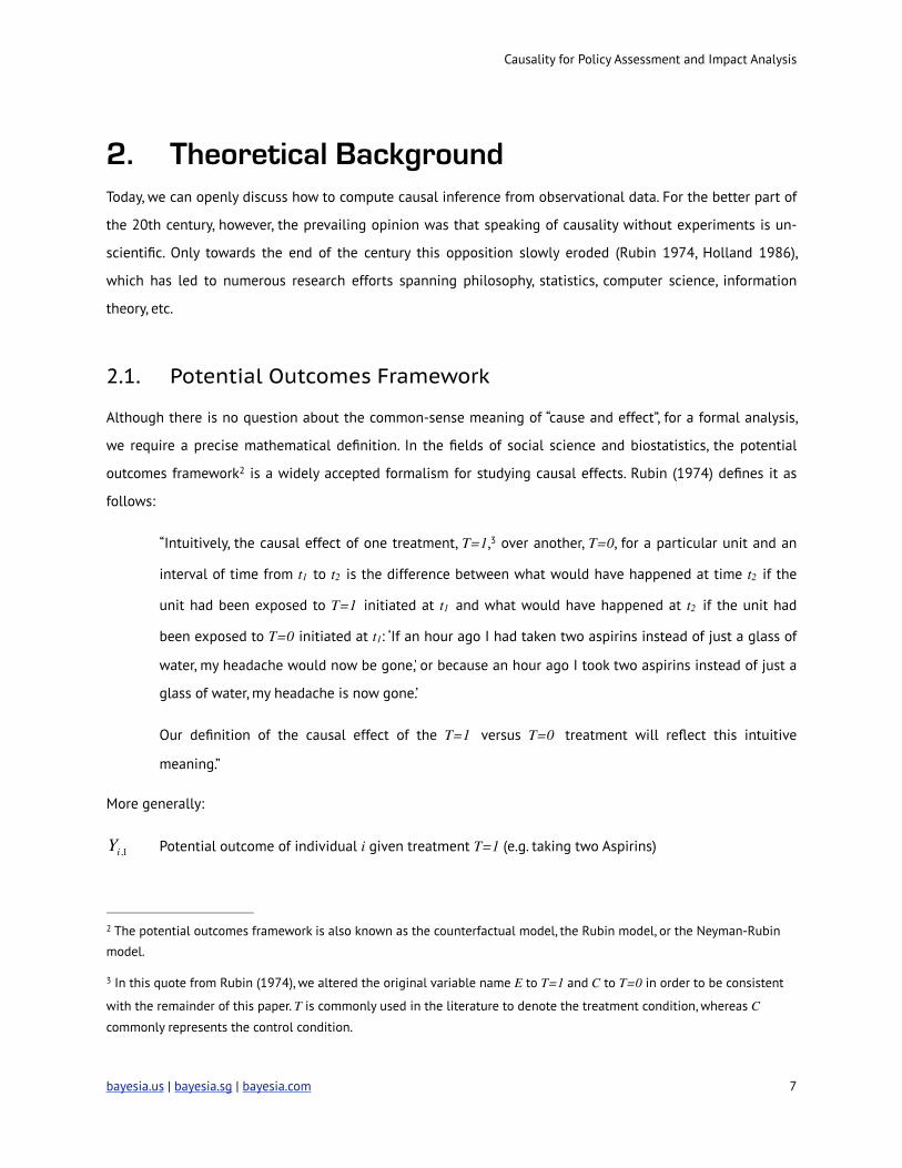
“Intuitively, the causal effect of one treatment, T=1, over another, T=0, for a particular unit and an 3

interval of time from t1 to t2 is the difference between what would have happened at time t2 if the

unit had been exposed to T=1 initiated at t1 and what would have happened at t2 if the unit had

been exposed to T=0 initiated at t1: ‘If an hour ago I had taken two aspirins instead of just a glass of

water, my headache would now be gone,' or because an hour ago I took two aspirins instead of just a

glass of water, my headache is now gone.’

Our definition of the causal effect of the T=1 versus T=0 treatment will reflect this intuitive

meaning.”

More generally:

! Potential outcome of individual i given treatment T=1 (e.g. taking two Aspirins) Yi,1

The potential outcomes framework is also known as the counterfactual model, the Rubin model, or the Neyman-Rubin 2

model.

In this quote from Rubin (1974), we altered the original variable name E to T=1 and C to T=0 in order to be consistent 3

with the remainder of this paper. T is commonly used in the literature to denote the treatment condition, whereas C

commonly represents the control condition.






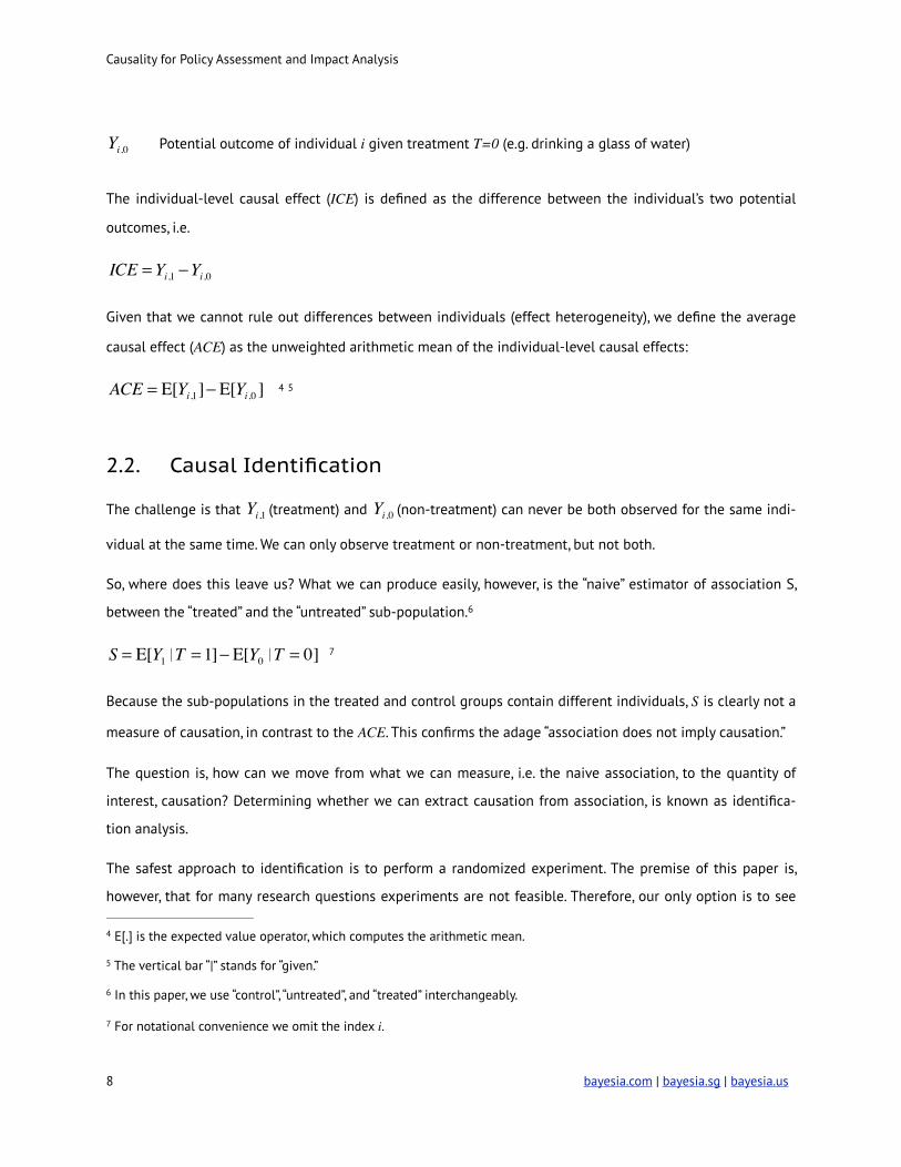
Potential outcome of individual i given treatment T=0 (e.g. drinking a glass of water)

The individual-level causal effect (ICE) is defined as the difference between the individual’s two potential

outcomes, i.e.

!

Given that we cannot rule out differences between individuals (effect heterogeneity), we define the average

causal effect (ACE) as the unweighted arithmetic mean of the individual-level causal effects:

4 5

2.2. Causal Identification

The challenge is that ! (treatment) and ! (non-treatment) can never be both observed for the same indi-

vidual at the same time. We can only observe treatment or non-treatment, but not both.

So, where does this leave us? What we can produce easily, however, is the “naive” estimator of association S,

between the “treated” and the “untreated” sub-population. 6

7

Because the sub-populations in the treated and control groups contain different individuals, S is clearly not a

measure of causation, in contrast to the ACE. This confirms the adage “association does not imply causation.”

The question is, how can we move from what we can measure, i.e. the naive association, to the quantity of

interest, causation? Determining whether we can extract causation from association, is known as identifica-

tion analysis.

The safest approach to identification is to perform a randomized experiment. The premise of this paper is,

however, that for many research questions experiments are not feasible. Therefore, our only option is to see

Yi,0

ICE = Yi,1 −Yi,0

ACE = E[Yi,1]− E[Yi,0 ]

Yi,1 Yi,0

S = E[Y1�T = 1]− E[Y0�T = 0]

E[.] is the expected value operator, which computes the arithmetic mean.4

The vertical bar “|” stands for “given.”5

In this paper, we use “control”, “untreated”, and “treated” interchangeably. 6

For notational convenience we omit the index i.7






whether there are any conditions, under which the measure for association equals the measure of causation.

This will be the case when the sub-populations are comparable with respect to the factors that can influence

the outcome.

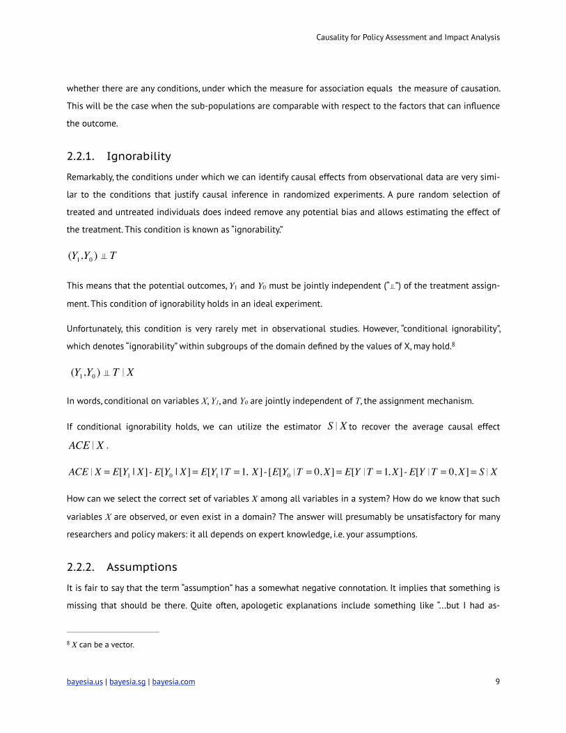
2.2.1. Ignorability

Remarkably, the conditions under which we can identify causal effects from observational data are very simi-

lar to the conditions that justify causal inference in randomized experiments. A pure random selection of

treated and untreated individuals does indeed remove any potential bias and allows estimating the effect of

the treatment. This condition is known as “ignorability.”

!

This means that the potential outcomes, Y1 and Y0 must be jointly independent (“a”) of the treatment assign-

ment. This condition of ignorability holds in an ideal experiment.

Unfortunately, this condition is very rarely met in observational studies. However, “conditional ignorability”,

which denotes “ignorability” within subgroups of the domain defined by the values of X, may hold. 8

!

In words, conditional on variables X, Y1, and Y0 are jointly independent of T, the assignment mechanism.

If conditional ignorability holds, we can utilize the estimator ! to recover the average causal effect

! .

How can we select the correct set of variables X among all variables in a system? How do we know that such

variables X are observed, or even exist in a domain? The answer will presumably be unsatisfactory for many

researchers and policy makers: it all depends on expert knowledge, i.e. your assumptions.

2.2.2. Assumptions

It is fair to say that the term “assumption” has a somewhat negative connotation. It implies that something is

missing that should be there. Quite often, apologetic explanations include something like “...but I had as-

(Y1,Y0 ) a T

(Y1,Y0 ) a T�X

�S�X

�ACE�X

ACE�X = E[Y1 | X]-E[Y0 | X]= E[Y1 |T = 1, X]-[E[Y0�T = 0,X]= E[Y�T = 1,X]-E[Y�T = 0,X]= S�X

X can be a vector.8






sumed that...” Even in science, assumptions can be relegated to footnotes or not even mentioned at all. Who,

for instance, lists all the assumptions made whenever OLS estimation is performed? Thus, assumptions are

often at the margins of research rather than at the core. The assumptions we use for the purposes of identifi-

cation, however, play a crucial role.

Causal inference requires causal assumptions. Specifically, analysts must make causal assumptions about the

process that generated the observed data (Manski 1995, Elwert 2013).

3. Methods for Identification and Estimation

3.1. Directed Acyclic Graphs for Identification

In this section, all assumptions for identification are expressed explicitly by means of a Directed Acyclic Graph

(DAG) (Pearl 1995, 2009).

So, what do we need to assume? We need to assume a causal model of our problem domain. These assump-

tions are not merely checkboxes to tick; rather, they represent our complete causal understanding of the data-

generating process for the system we are studying.

Where do we get such causal assumptions for a model? In this day and age when Big Data dominates the

headlines, we would like to say that advanced algorithms can generate causal assumptions from data. That is,

unfortunately, not the case. Structural, causal assumptions still require human expert knowledge, or, more

generally, theory. 9

In practice, this means that we need to build (or draw) a causal graph of our domain, which we can subse-

quently examine with regard to identification.

Later in this paper, we will present how machine learning can assist in building models.9






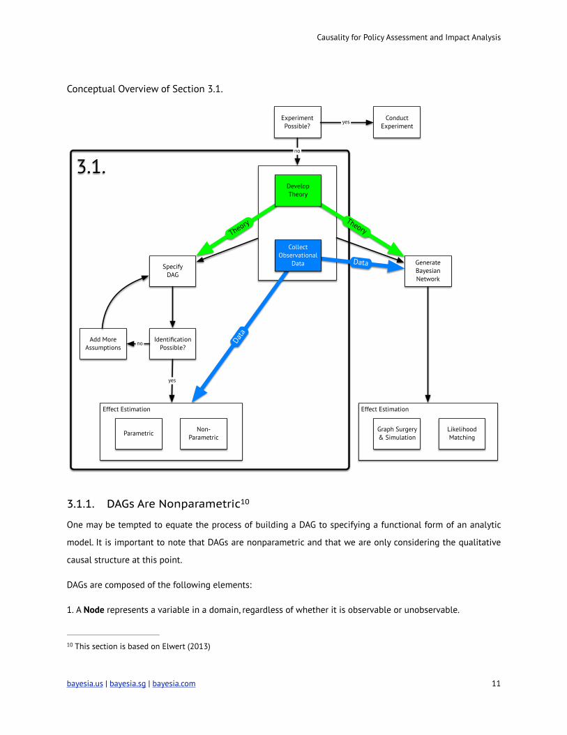
Conceptual Overview of Section 3.1.

!

3.1.1. DAGs Are Nonparametric 10

One may be tempted to equate the process of building a DAG to specifying a functional form of an analytic

model. It is important to note that DAGs are nonparametric and that we are only considering the qualitative

causal structure at this point.

DAGs are composed of the following elements:

1. A Node represents a variable in a domain, regardless of whether it is observable or unobservable.

3.1.

Effect EstimationEffect Estimation

Experiment Possible?

Conduct Experiment

IdentificationPossible?

yes

Add MoreAssumptions

no

yes

SpecifyDAG

ParametricGraph Surgery & Simulation

Non-Parametric

LikelihoodMatching

GenerateBayesian Network

no

Theory

Data

Data

Theory

CollectObservational

Data

Develop Theory

This section is based on Elwert (2013)10






2. A Directed Arc has the appearance of an arrow and represents a potential causal effect. The arc direction

indicates the assumed causal direction, i.e. “A→B” means “A causes B.”

3. A Missing Arc encodes the definitive absence of a direct causal effect, i.e. no arc between A and B means

that there exists no direct causal relationship between A and B and vice versa. As such, a missing arc repre-

sents an assumption.

3.1.2. Structures within a DAG

In a DAG, there are three basic configurations in which nodes can be connected. DAGs of any size and com-

plexity can be broken down into these basic graph structures, which primarily express causal effects between

nodes.

While these basic structures show direct causes explicitly, there are more statements contained in them, al-

beit implicitly. In fact, we can read all marginal and conditional associations that exist between the nodes.

Why are we even interested in associations? Isn’t all this about understanding causal effects? Actually, it is

essential to understand all associations in a system because we can only observe associations in observed

data, and some of these associations can represent non-causal relationships. Our objective is to separate

causal effects from non-causal associations.

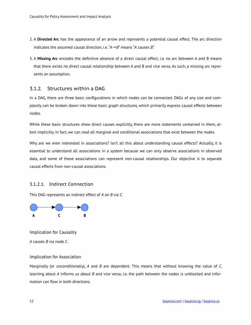
3.1.2.1. Indirect Connection

This DAG represents an indirect effect of A on B via C.

!

Implication for Causality

A causes B via node C.

Implication for Association

Marginally (or unconditionally), A and B are dependent. This means that without knowing the value of C,

learning about A informs us about B and vice versa, i.e. the path between the nodes is unblocked and infor-

mation can flow in both directions.






Conditionally on C, i.e. by setting Hard Evidence on (or observing) C, A and B become independent. In other 11

words, by “hard”-conditioning on C, we block the path from A to B and from B to A. Thus, A and B are rendered

independent, given C.

!

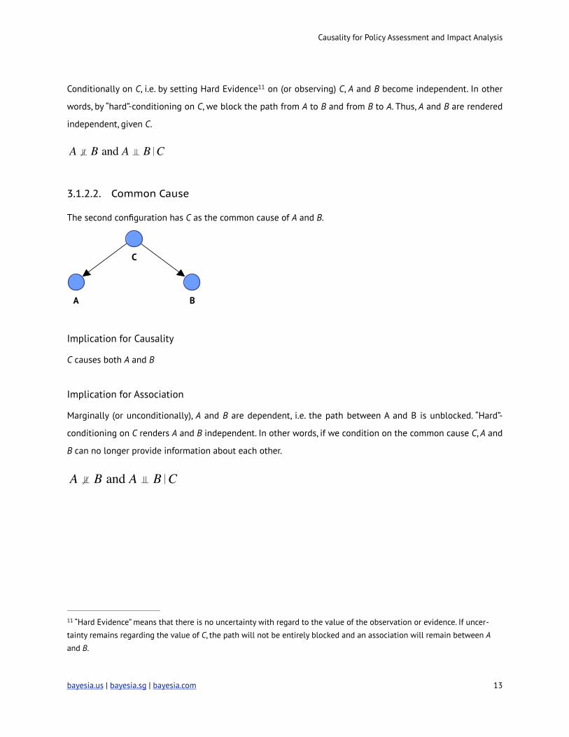
3.1.2.2. Common Cause

The second configuration has C as the common cause of A and B.

!


C causes both A and B


Marginally (or unconditionally), A and B are dependent, i.e. the path between A and B is unblocked. “Hard”-

conditioning on C renders A and B independent. In other words, if we condition on the common cause C, A and

B can no longer provide information about each other.

!

�A b B and A a B�C

�A b B and A a B�C

“Hard Evidence” means that there is no uncertainty with regard to the value of the observation or evidence. If uncer11 -

tainty remains regarding the value of C, the path will not be entirely blocked and an association will remain between A

and B.






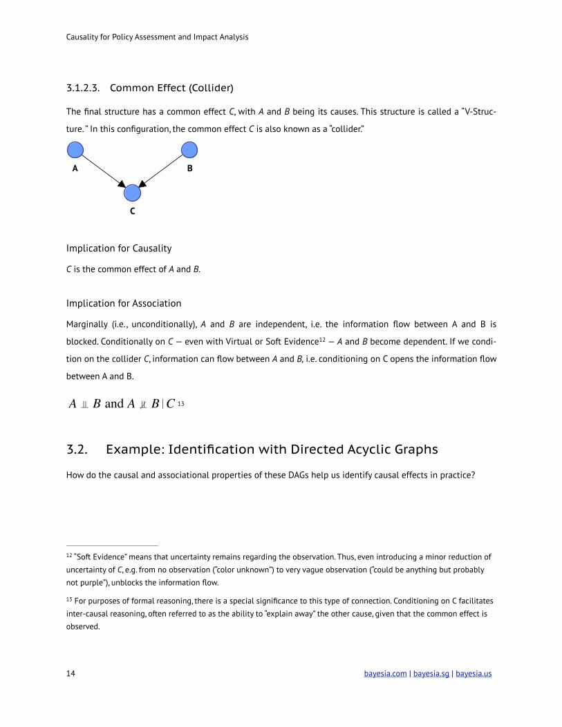
3.1.2.3. Common Effect (Collider)

The final structure has a common effect C, with A and B being its causes. This structure is called a “V-Struc-

ture. ” In this configuration, the common effect C is also known as a “collider.”

!


C is the common effect of A and B.


Marginally (i.e., unconditionally), A and B are independent, i.e. the information flow between A and B is

blocked. Conditionally on C — even with Virtual or Soft Evidence — A and B become dependent. If we condi12 -

tion on the collider C, information can flow between A and B, i.e. conditioning on C opens the information flow

between A and B.

13

3.2. Example: Identification with Directed Acyclic Graphs

How do the causal and associational properties of these DAGs help us identify causal effects in practice?

�A a B and A b B�C

“Soft Evidence” means that uncertainty remains regarding the observation. Thus, even introducing a minor reduction of 12

uncertainty of C, e.g. from no observation (“color unknown”) to very vague observation (“could be anything but probably

not purple”), unblocks the information flow.

For purposes of formal reasoning, there is a special significance to this type of connection. Conditioning on C facilitates 13

inter-causal reasoning, often referred to as the ability to “explain away” the other cause, given that the common effect is

observed.






3.2.1. Example: Simpson’s Paradox

We will use an example that appears trivial on the surface, but which has produced countless instances of

false inference throughout the history of science. Due to its counterintuitive nature, this example has become

widely known as Simpson’s Paradox.

This is an important exercise as it illustrates how an incorrect interpretation of association can produce bias.

The word “bias” may not necessarily strike fear into our hearts. In our common understanding, “bias” implies

“inclination” and “tendency”, and it is certainly not a particularly forceful expression. Hence, we may not be

overly concerned by a warning about bias. However, Simpson’s Paradox shows how bias can lead to cat-

astrophically wrong estimates.

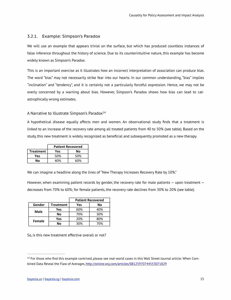
A Narrative to Illustrate Simpson’s Paradox 14

A hypothetical disease equally affects men and women. An observational study finds that a treatment is

linked to an increase of the recovery rate among all treated patients from 40 to 50% (see table). Based on the

study, this new treatment is widely recognized as beneficial and subsequently promoted as a new therapy.

!

We can imagine a headline along the lines of “New Therapy Increases Recovery Rate by 10%.”

However, when examining patient records by gender, the recovery rate for male patients — upon treatment —

decreases from 70% to 60%; for female patients, the recovery rate declines from 30% to 20% (see table).

!

So, is this new treatment effective overall or not?

Treatment Yes NoYes 50% 50%No 40% 60%

Patient.Recovered

Gender Treatment Yes NoYes 60% 40%No 70% 30%Yes 20% 80%No 30% 70%

Patient0Recovered

Male

Female

For those who find this example contrived, please see real-world cases in this Wall Street Journal article: When Com14 -

bined Data Reveal the Flaw of Averages, http://online.wsj.com/articles/SB125970744553071829


http://online.wsj.com/articles/SB125970744553071829





This puzzle can be resolved by realizing that, in this observed population, there was an unequal application of

the treatment to men and women, i.e. some type of self-selection occurred. More specifically, 75% of the male

patients and only 25% of female patients received the treatment. Although the reason for this imbalance is

irrelevant for inference, one could imagine that side effects of this treatment are much more severe for fe-

males, who thus seek alternatives therapies. As a result, there is a greater share of men among the treated

patients. Given that men have a better a priori recovery prospect with this type of disease, the recovery rate

for the total patient population increases.

So, what is the true causal effect of this treatment?

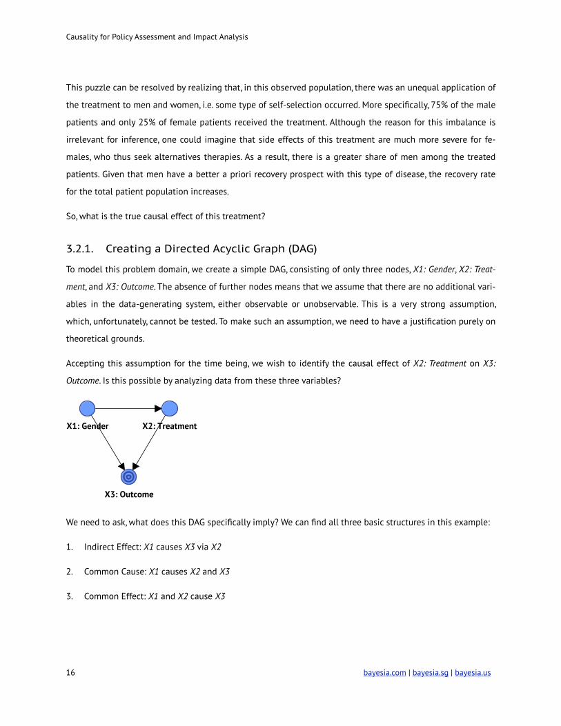
3.2.1. Creating a Directed Acyclic Graph (DAG)

To model this problem domain, we create a simple DAG, consisting of only three nodes, X1: Gender, X2: Treat-

ment, and X3: Outcome. The absence of further nodes means that we assume that there are no additional vari-

ables in the data-generating system, either observable or unobservable. This is a very strong assumption,

which, unfortunately, cannot be tested. To make such an assumption, we need to have a justification purely on

theoretical grounds.

Accepting this assumption for the time being, we wish to identify the causal effect of X2: Treatment on X3:

Outcome. Is this possible by analyzing data from these three variables?

!

We need to ask, what does this DAG specifically imply? We can find all three basic structures in this example:

1. Indirect Effect: X1 causes X3 via X2

2. Common Cause: X1 causes X2 and X3

3. Common Effect: X1 and X2 cause X3






3.1.1. Graphical Identification Criteria

Earlier we said that we also need to understand all the associations in a system, so we can distinguish be-

tween causation and association. This requirement will perhaps become clearer now as we introduce the con-

cepts of causal and non-causal paths.

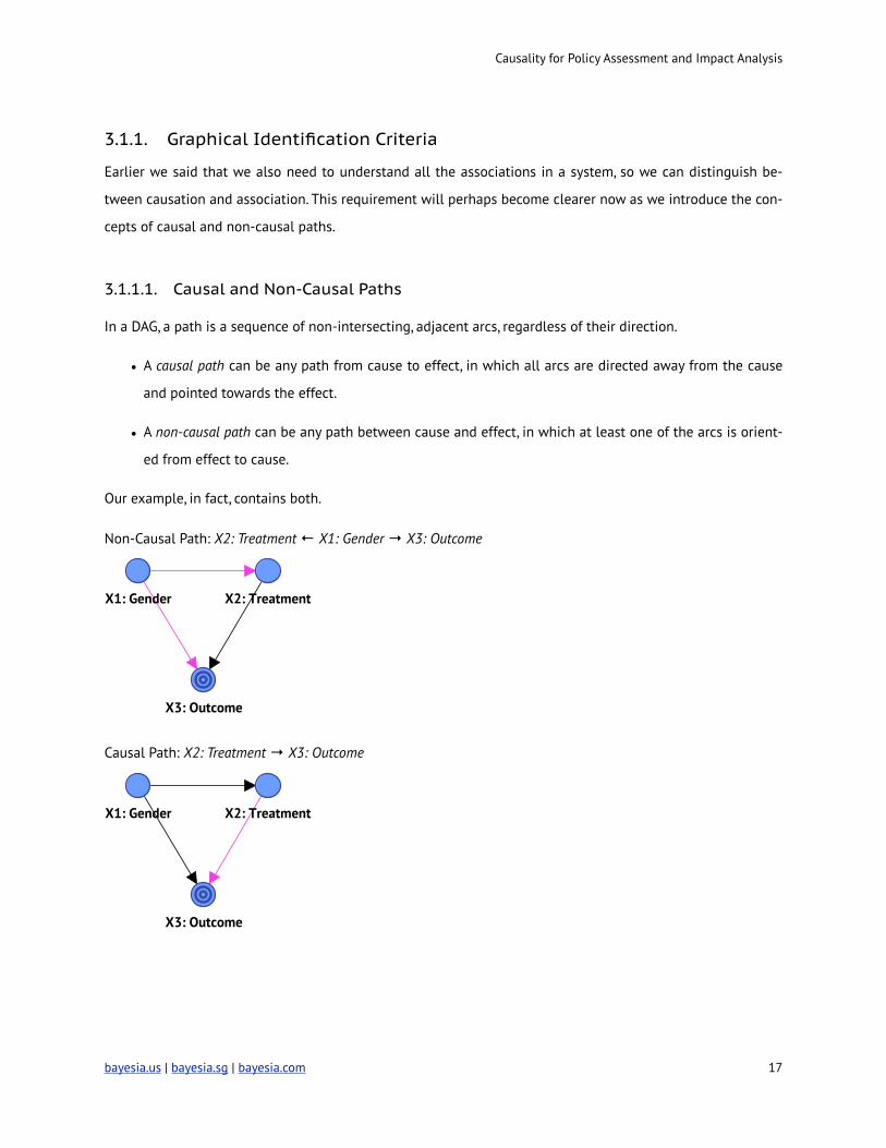
3.1.1.1. Causal and Non-Causal Paths

In a DAG, a path is a sequence of non-intersecting, adjacent arcs, regardless of their direction.

• A causal path can be any path from cause to effect, in which all arcs are directed away from the cause

and pointed towards the effect.

• A non-causal path can be any path between cause and effect, in which at least one of the arcs is orient-

ed from effect to cause.

Our example, in fact, contains both.

Non-Causal Path: X2: Treatment ← X1: Gender → X3: Outcome

!

Causal Path: X2: Treatment → X3: Outcome

!






Among numerous available graphical criteria, the Adjustment Criterion (Shpitser et al. 2010) is perhaps the

most intuitive one. Put simply, the Adjustment Criterion states that a causal effect is identified, if we can con-

dition on (adjust for) a set of nodes such that:

• All non-causal paths between treatment and effect are “blocked” (non-causal relationships prevented).

• All causal paths from treatment to effect remain “open” (causal relationships preserved).

This means that any association that we can measure after adjustment in our data must be causal, which is

precisely what we wish to know.

What does “adjust for” mean in practice? In this context, “adjusting for a variable” and “conditioning on a vari-

able” are interchangeable. They can stand for any of the following operations, which all introduce information

on a variable, e.g.:

• Controlling

• Stratifying

• Setting evidence

• Observing

• Matching

At this point, the adjustment technique is irrelevant. Rather, we just need to determine which variables, if any,

need to be adjusted for in order to block the non-causal paths while keeping the causal paths open.

Revisiting both paths in our DAG, we can now examine which ones are open or blocked. First, we look at the

non-causal path in our DAG.

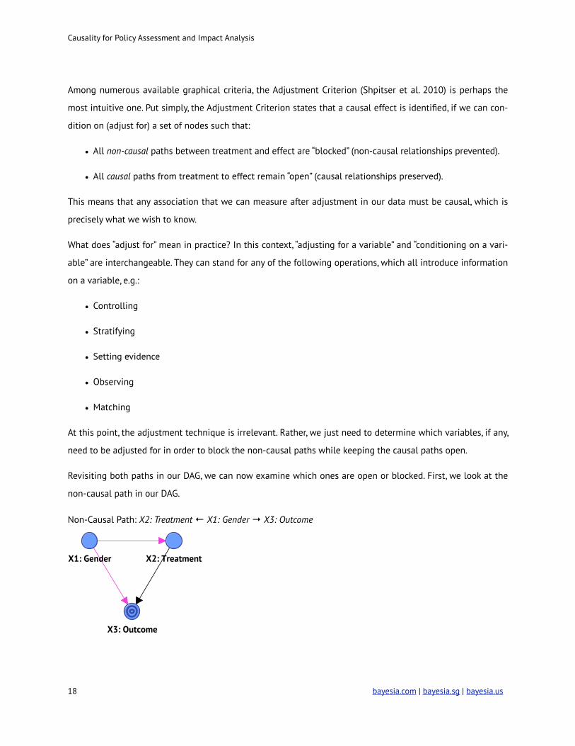
Non-Causal Path: X2: Treatment ← X1: Gender → X3: Outcome

!






X1 is a common cause of X2 and X3. This implies that there is an indirect association between X2 and X3.

Hence, there is an open non-causal path between X2 and X3, which has to be blocked. To block this path, we

simply need to adjust for X1.

Next is the causal path in our DAG.

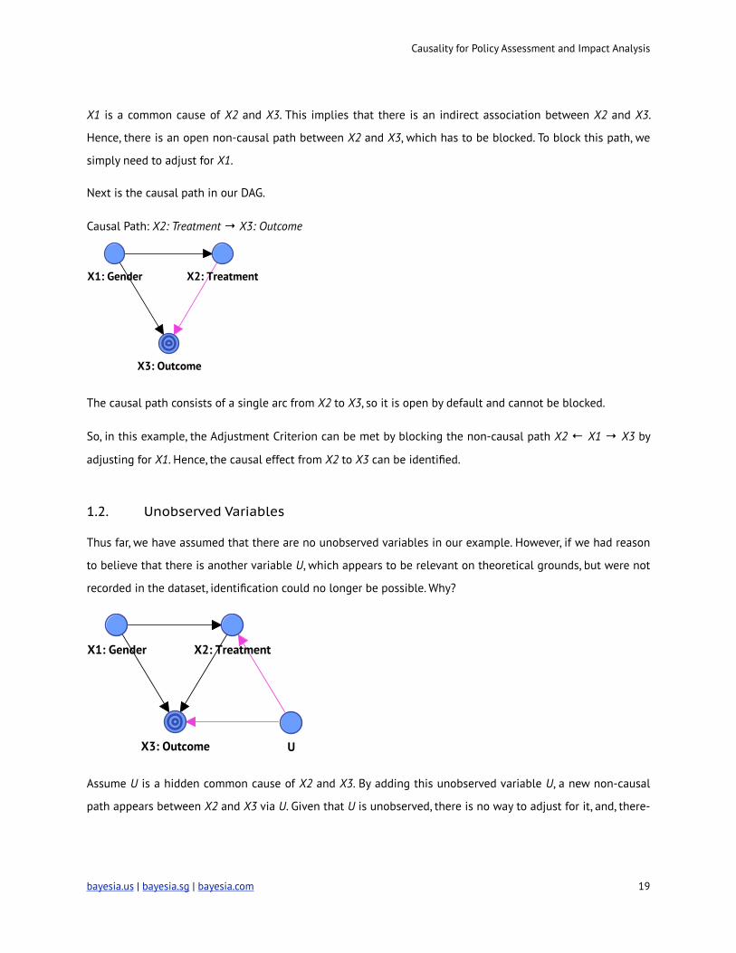
Causal Path: X2: Treatment → X3: Outcome

!

The causal path consists of a single arc from X2 to X3, so it is open by default and cannot be blocked.

So, in this example, the Adjustment Criterion can be met by blocking the non-causal path X2 ← X1 → X3 by

adjusting for X1. Hence, the causal effect from X2 to X3 can be identified.

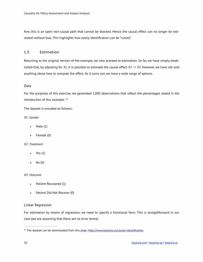
1.2. Unobserved Variables

Thus far, we have assumed that there are no unobserved variables in our example. However, if we had reason

to believe that there is another variable U, which appears to be relevant on theoretical grounds, but were not

recorded in the dataset, identification could no longer be possible. Why?

!

Assume U is a hidden common cause of X2 and X3. By adding this unobserved variable U, a new non-causal

path appears between X2 and X3 via U. Given that U is unobserved, there is no way to adjust for it, and, there-






fore, this is an open non-causal path that cannot be blocked. Hence, the causal effect can no longer be esti-

mated without bias. This highlights how easily identification can be “ruined.”

1.3. Estimation

Returning to the original version of the example, we now proceed to estimation. So far, we have simply estab-

lished that, by adjusting for X1, it is possible to estimate the causal effect X2 → X3. However, we have not said

anything about how to compute the effect. As it turns out, we have a wide range of options.

Data

For the purposes of this exercise, we generated 1,000 observations that reflect the percentages stated in the

introduction of this example. 15

The dataset is encoded as follows:

X1: Gender

• Male (1)

• Female (0)

X2: Treatment

• Yes (1)

• No (0)

X3: Outcome

• Patient Recovered (1)

• Patient Did Not Recover (0)

Linear Regression

For estimation by means of regression, we need to specify a functional form. This is straightforward in our

case (we are assuming that there are no error terms):

The dataset can be downloaded from this page: http://www.bayesia.us/causal-identification15


http://www.bayesia.us/causal-identification





!

This function indeed provides what we need. By including X1 as a covariate (or independent variable), we au-

tomatically condition on it, which is required by the adjustment criterion. By estimating the regression, we are

conditioning on all the variables that are on the right-hand side of the equation.

The OLS estimation then yields the following coefficients:

!

We can now interpret the coefficient ! as the total causal effect of X2 on X3, and it turns out to be a nega-

tive effect! So, this causal analysis, which now removes bias by taking into account X1: Gender, yields the op-

posite effect of the one we would get by merely looking at association, i.e. -10% instead of +10% in recovery

rate.

Catastrophic Bias

Bias in effect estimation can be more than just a nuisance for the analyst; bias can reverse the sign of the

effect. In conditions similar to Simpson’s Paradox, effect estimates can be substantially wrong and lead to

policies with catastrophic consequences. In our example, the treatment under study kills people, instead of

healing them, as the naïve study based on association first suggested.

Other Effects

Perhaps we are now tempted to interpret ! as the total causal effect of X1 on X3. This would not be correct.

Instead, ! corresponds to the direct causal effect of X1 on X3.

If we want to identify the total causal effect of X1 on X3, we will need to look once again at the paths in our

DAG.

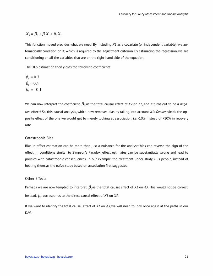
X3 = β0 + β1X1 + β2X2

β0 = 0.3β1 = 0.4β2 = −0.1

β2

β1

β1






!

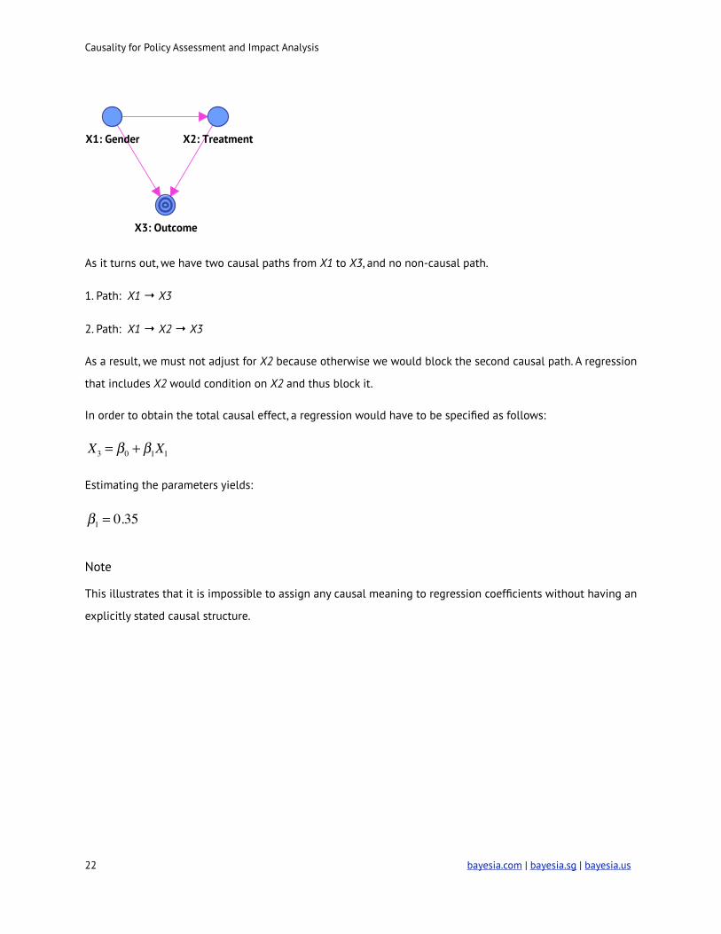
As it turns out, we have two causal paths from X1 to X3, and no non-causal path.

1. Path: X1 → X3

2. Path: X1 → X2 → X3

As a result, we must not adjust for X2 because otherwise we would block the second causal path. A regression

that includes X2 would condition on X2 and thus block it.

In order to obtain the total causal effect, a regression would have to be specified as follows:

!

Estimating the parameters yields:

!

Note

This illustrates that it is impossible to assign any causal meaning to regression coefficients without having an

explicitly stated causal structure.

X3 = β0 + β1X1

β1 = 0.35






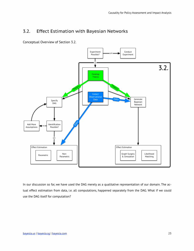
3.2. Effect Estimation with Bayesian Networks

Conceptual Overview of Section 3.2.

!

In our discussion so far, we have used the DAG merely as a qualitative representation of our domain. The ac-

tual effect estimation from data, i.e. all computations, happened separately from the DAG. What if we could

use the DAG itself for computation?

3.2.

Effect EstimationEffect Estimation

Experiment Possible?

Conduct Experiment

IdentificationPossible?

yes

Add MoreAssumptions

no

yes

SpecifyDAG

ParametricGraph Surgery & Simulation

Non-Parametric

LikelihoodMatching

GenerateBayesian Network

no

Theory

Data

Data

Theory

CollectObservational

Data

Develop Theory






3.2.1. Creating a Bayesian Network from a DAG and Data

In fact, this type of DAG exists. It is called a Bayesian network. Beyond the structure of the DAG, a Bayesian

network contains marginal or conditional probability distributions for each variable.

How do we obtain these distributions? By using Maximum Likelihood, i.e. counting the (co-)occurrences of the

states of the variables in our data:

!

Counting all 1,000 records, we obtain the marginal count of each state of X1.

!

Given that our DAG structure says that X1 causes X2, we will now count the states of X2 conditional on X1.

This is simply a cross-tabulation.

!

Finally, we count the states of X3 conditional on its causes X1 and X2. In Excel, this could be done with a Piv-

ot Table, for instance.

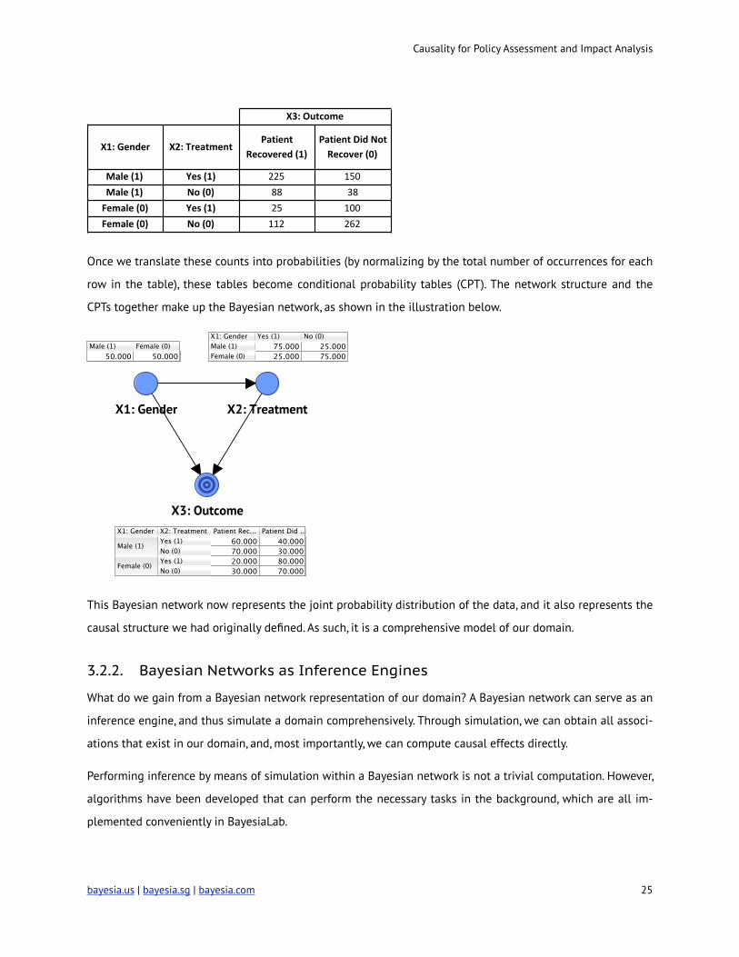
X1:$Gender X2:$Treatment X3:$Outcome CountMale%(1) Yes%(1) Patient%Recovered%(1) 225Male%(1) Yes%(1) Patient%Did%Not%Recover%(0) 150Male%(1) No%(0) Patient%Recovered%(1) 88Male%(1) No%(0) Patient%Did%Not%Recover%(0) 38Female%(0) Yes%(1) Patient%Recovered%(1) 25Female%(0) Yes%(1) Patient%Did%Not%Recover%(0) 100Female%(0) No%(0) Patient%Recovered%(1) 112Female%(0) No%(0) Patient%Did%Not%Recover%(0) 262

Female&(0) Male&(1)500 500

X1:&Gender

No#(0) Yes#(1)Female#(0) 750 250Male#(1) 250 750

X2:#Treatment

X1:#Gender






!

Once we translate these counts into probabilities (by normalizing by the total number of occurrences for each

row in the table), these tables become conditional probability tables (CPT). The network structure and the

CPTs together make up the Bayesian network, as shown in the illustration below.

!

This Bayesian network now represents the joint probability distribution of the data, and it also represents the

causal structure we had originally defined. As such, it is a comprehensive model of our domain.

3.2.2. Bayesian Networks as Inference Engines

What do we gain from a Bayesian network representation of our domain? A Bayesian network can serve as an

inference engine, and thus simulate a domain comprehensively. Through simulation, we can obtain all associ-

ations that exist in our domain, and, most importantly, we can compute causal effects directly.

Performing inference by means of simulation within a Bayesian network is not a trivial computation. However,

algorithms have been developed that can perform the necessary tasks in the background, which are all im-

plemented conveniently in BayesiaLab.

X1:$Gender X2:$TreatmentPatient$

Recovered$(1)Patient$Did$Not$Recover$(0)

Male$(1) Yes$(1) 225 150Male$(1) No$(0) 88 38Female$(0) Yes$(1) 25 100Female$(0) No$(0) 112 262

X3:$Outcome






3.2.3. Software Platform: BayesiaLab 5.3 Professional

As we continue with this example, we will use the BayesiaLab 5.3 Professional software package for all such

inference and simulation computations. In fact, all the network graphs shown in this paper were created with

BayesiaLab. Furthermore, the task of creating conditional probability tables from data is fully automated in

BayesiaLab. The remainder of this paper is in the form of a tutorial, which encourages you to follow along

every step, using your BayesiaLab installation. 16

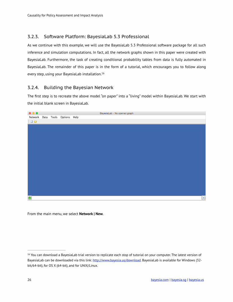
3.2.4. Building the Bayesian Network

The first step is to recreate the above model “on paper” into a “living” model within BayesiaLab. We start with

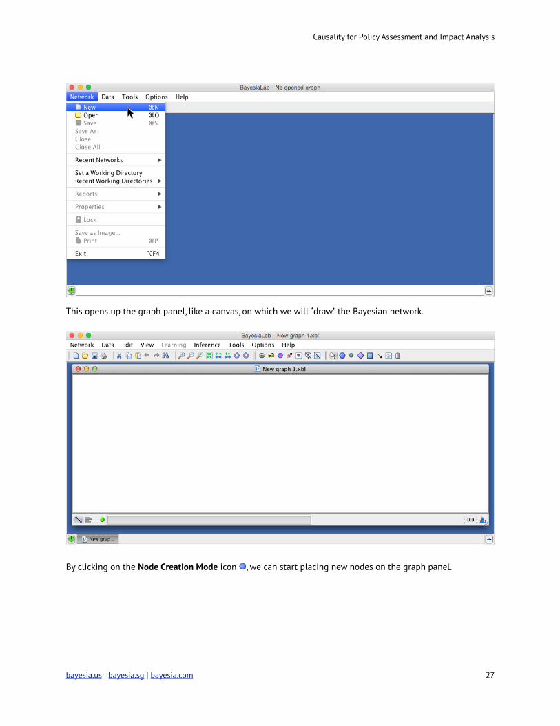
the initial blank screen in BayesiaLab.

!

From the main menu, we select Network | New.

You can download a BayesiaLab trial version to replicate each stop of tutorial on your computer. The latest version of 16

BayesiaLab can be downloaded via this link: http://www.bayesia.us/download. BayesiaLab is available for Windows (32-

bit/64-bit), for OS X (64-bit), and for UNIX/Linux.


http://www.bayesia.us/download





!

This opens up the graph panel, like a canvas, on which we will “draw” the Bayesian network.

!

By clicking on the Node Creation Mode icon ! , we can start placing new nodes on the graph panel.






!

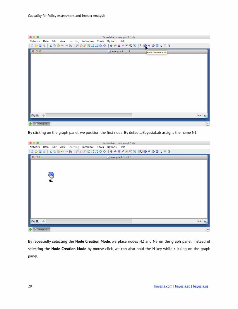
By clicking on the graph panel, we position the first node. By default, BayesiaLab assigns the name N1.

!

By repeatedly selecting the Node Creation Mode, we place nodes N2 and N3 on the graph panel. Instead of

selecting the Node Creation Mode by mouse-click, we can also hold the N-key while clicking on the graph

panel.






!

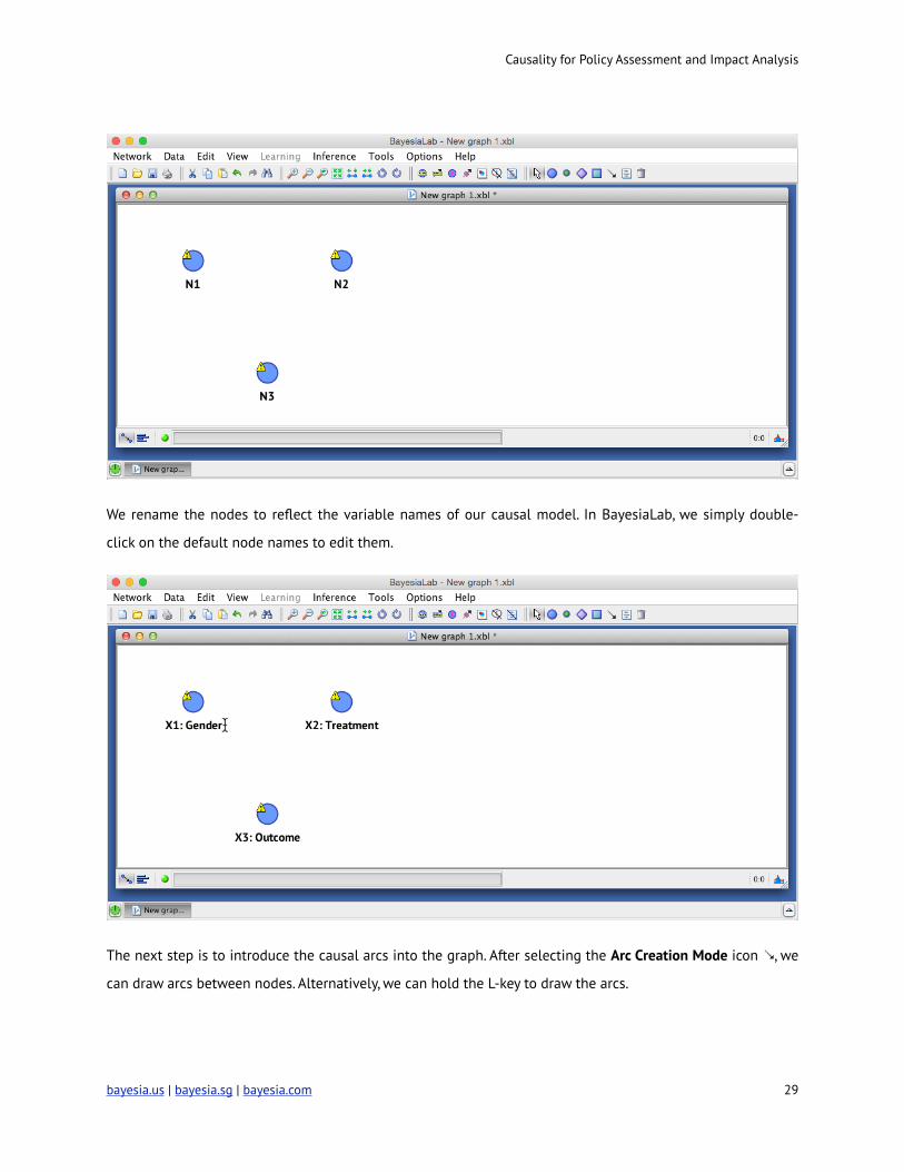
We rename the nodes to reflect the variable names of our causal model. In BayesiaLab, we simply double-

click on the default node names to edit them.

!

The next step is to introduce the causal arcs into the graph. After selecting the Arc Creation Mode icon ! , we

can draw arcs between nodes. Alternatively, we can hold the L-key to draw the arcs.






!

!

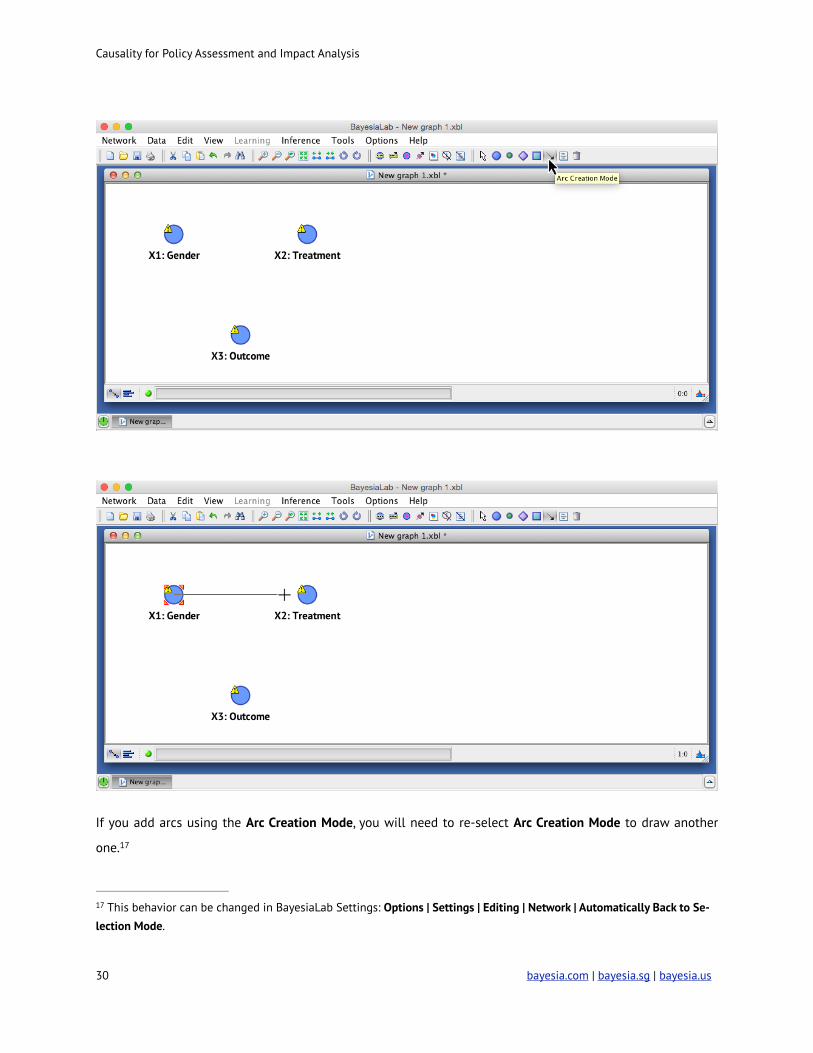
If you add arcs using the Arc Creation Mode, you will need to re-select Arc Creation Mode to draw another

one. 17

This behavior can be changed in BayesiaLab Settings: Options | Settings | Editing | Network | Automatically Back to Se17 -lection Mode.






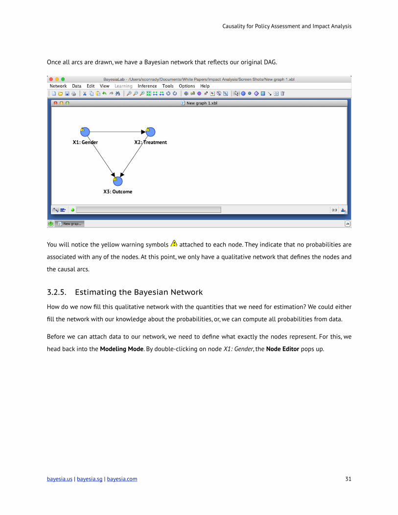
Once all arcs are drawn, we have a Bayesian network that reflects our original DAG.

!

You will notice the yellow warning symbols ! attached to each node. They indicate that no probabilities are

associated with any of the nodes. At this point, we only have a qualitative network that defines the nodes and

the causal arcs.

3.2.5. Estimating the Bayesian Network

How do we now fill this qualitative network with the quantities that we need for estimation? We could either

fill the network with our knowledge about the probabilities, or, we can compute all probabilities from data.

Before we can attach data to our network, we need to define what exactly the nodes represent. For this, we

head back into the Modeling Mode. By double-clicking on node X1: Gender, the Node Editor pops up.






!

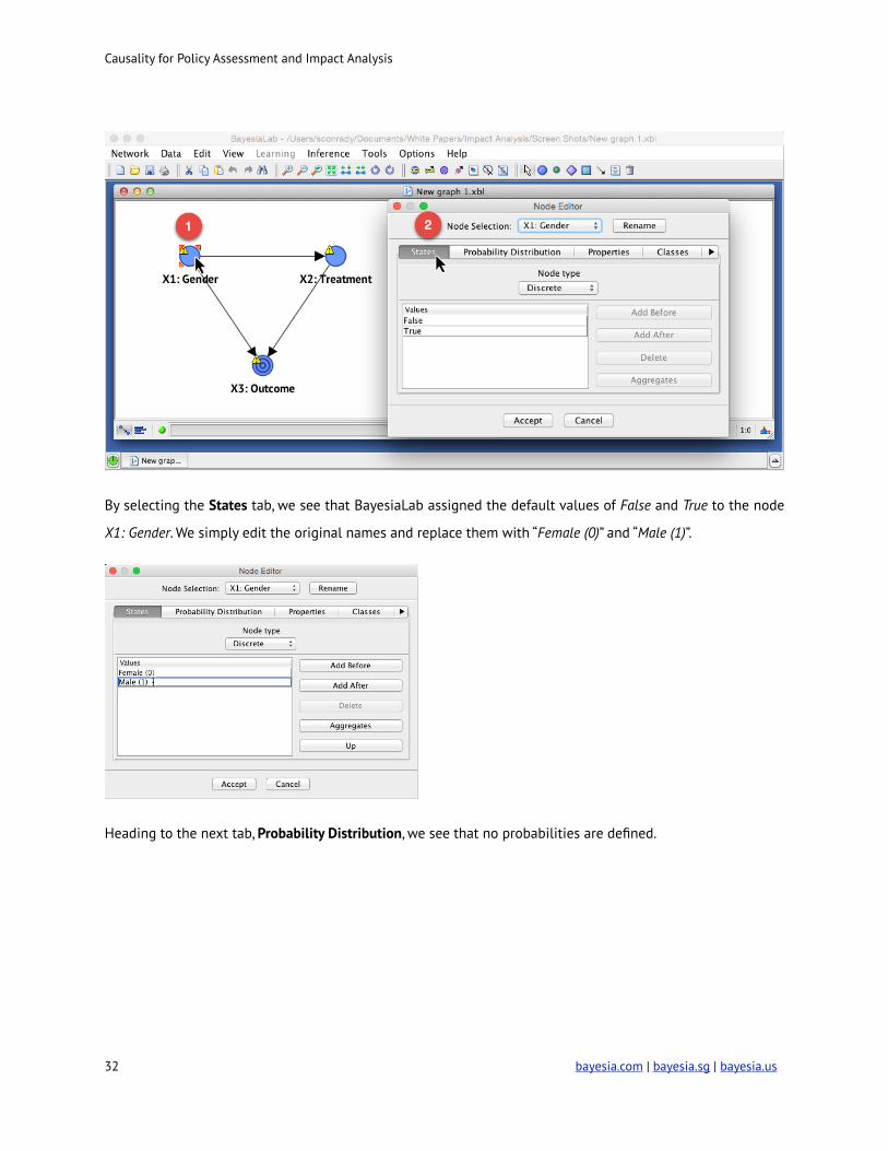
By selecting the States tab, we see that BayesiaLab assigned the default values of False and True to the node

X1: Gender. We simply edit the original names and replace them with “Female (0)” and “Male (1)”.

!

Heading to the next tab, Probability Distribution, we see that no probabilities are defined.






!

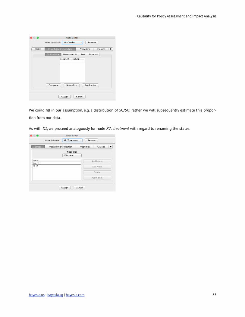
We could fill in our assumption, e.g. a distribution of 50/50; rather, we will subsequently estimate this propor-

tion from our data.

As with X1, we proceed analogously for node X2: Treatment with regard to renaming the states.

!






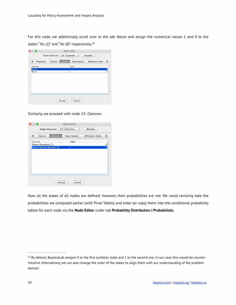
For this node, we additionally scroll over to the tab Values and assign the numerical values 1 and 0 to the

states “Yes (1)” and “No (0)” respectively. 18

!

Similarly, we proceed with node X3: Outcome.

!

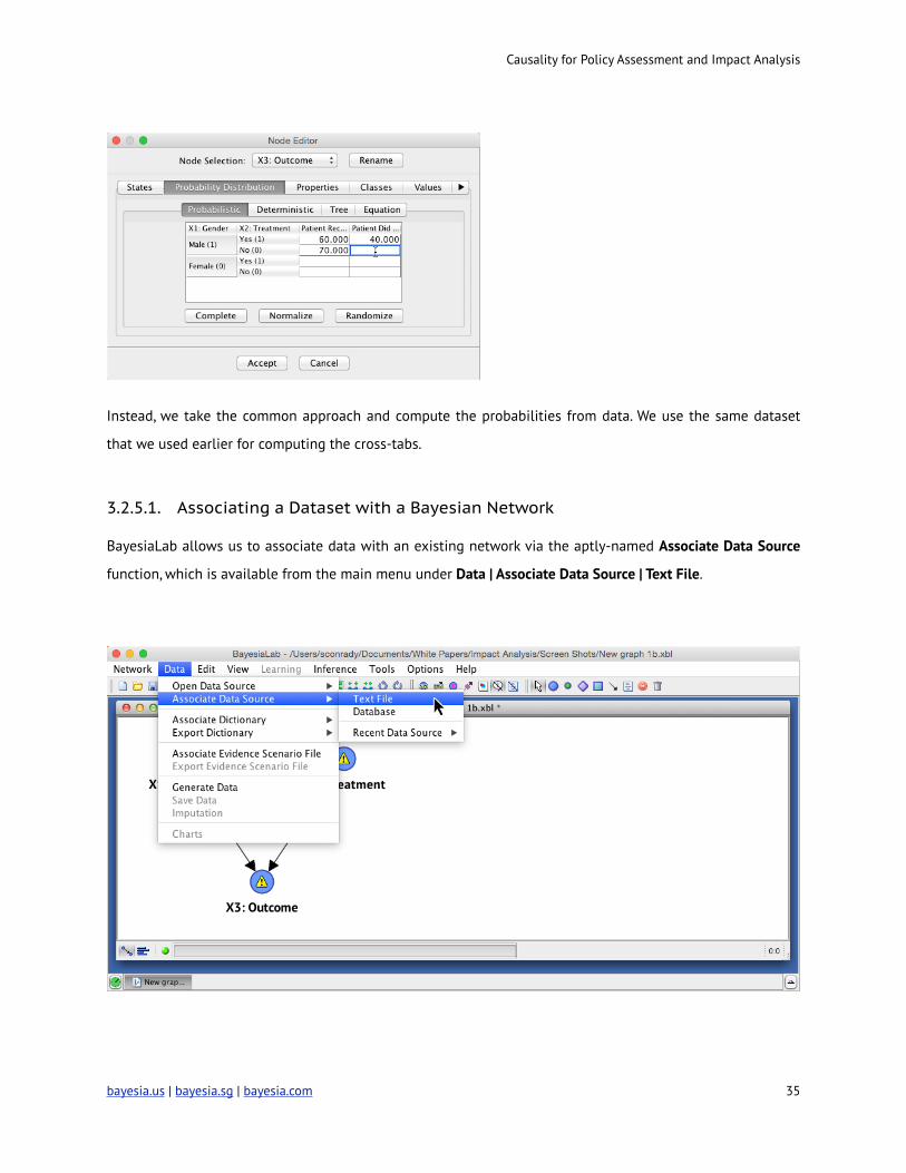
Now all the states of all nodes are defined; however, their probabilities are not. We could certainly take the

probabilities we computed earlier (with Pivot Tables) and enter (or copy) them into the conditional probability

tables for each node via the Node Editor under tab Probability Distribution | Probabilistic.

By default, BayesiaLab assigns 0 to the first symbolic state and 1 to the second one. In our case, this would be counter18 -

intuitive. Alternatively, we can also change the order of the states to align them with our understanding of the problem

domain






!

Instead, we take the common approach and compute the probabilities from data. We use the same dataset

that we used earlier for computing the cross-tabs.

3.2.5.1. Associating a Dataset with a Bayesian Network

BayesiaLab allows us to associate data with an existing network via the aptly-named Associate Data Source

function, which is available from the main menu under Data | Associate Data Source | Text File.

!






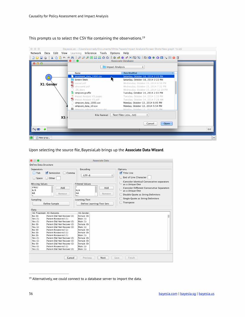
This prompts us to select the CSV file containing the observations. 19

!

Upon selecting the source file, BayesiaLab brings up the Associate Data Wizard.

!

Alternatively, we could connect to a database server to import the data. 19






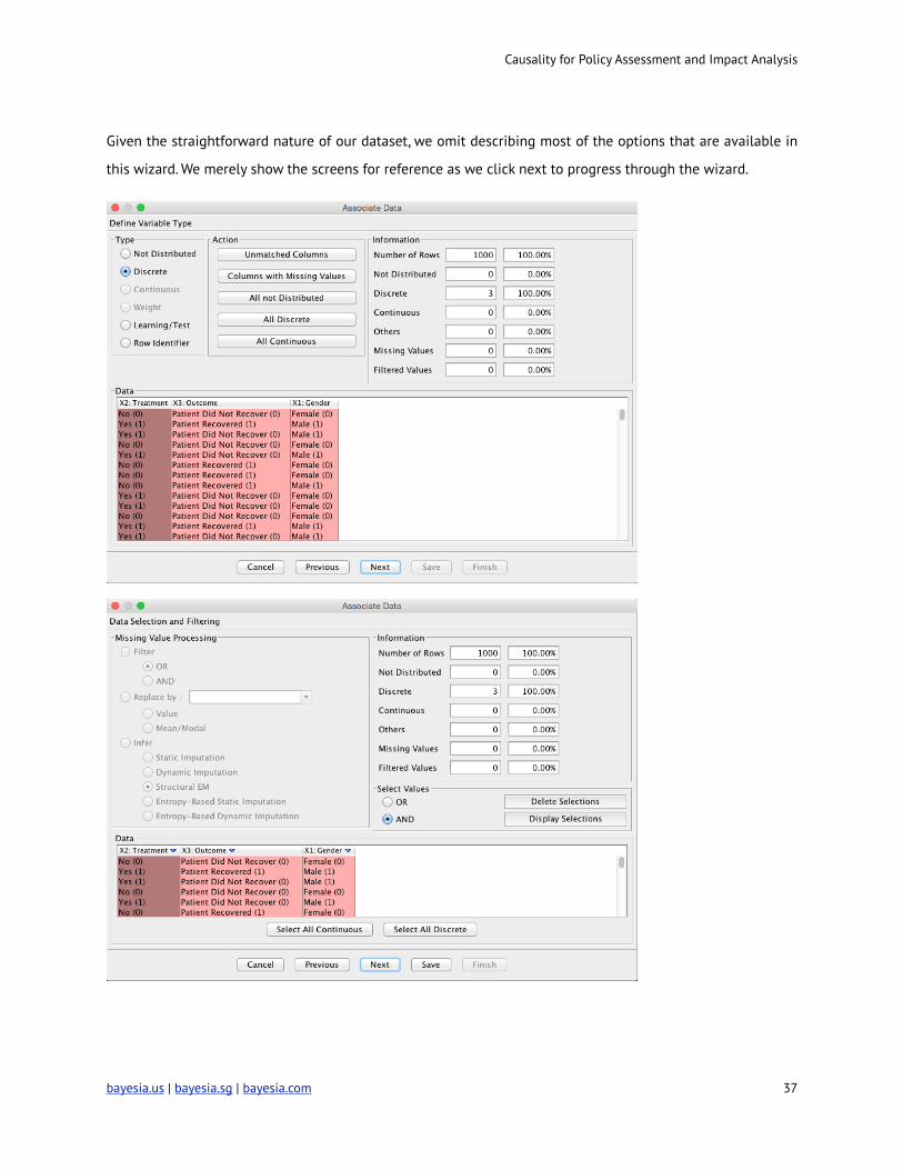
Given the straightforward nature of our dataset, we omit describing most of the options that are available in

this wizard. We merely show the screens for reference as we click next to progress through the wizard.

!

!






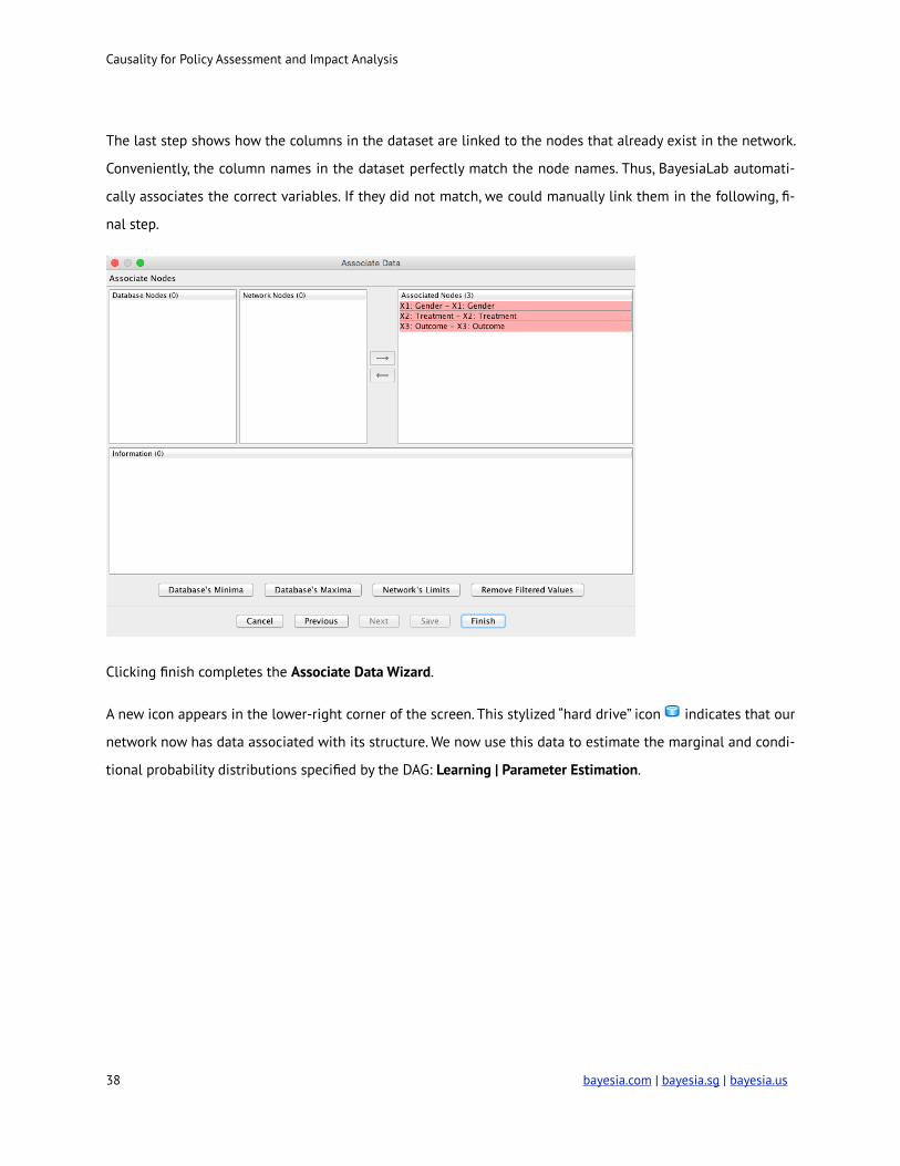
The last step shows how the columns in the dataset are linked to the nodes that already exist in the network.

Conveniently, the column names in the dataset perfectly match the node names. Thus, BayesiaLab automati-

cally associates the correct variables. If they did not match, we could manually link them in the following, fi-

nal step.

!

Clicking finish completes the Associate Data Wizard.

A new icon appears in the lower-right corner of the screen. This stylized “hard drive” icon ! indicates that our

network now has data associated with its structure. We now use this data to estimate the marginal and condi-

tional probability distributions specified by the DAG: Learning | Parameter Estimation.






!

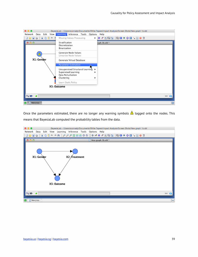
Once the parameters estimated, there are no longer any warning symbols ! tagged onto the nodes. This

means that BayesiaLab computed the probability tables from the data.

!






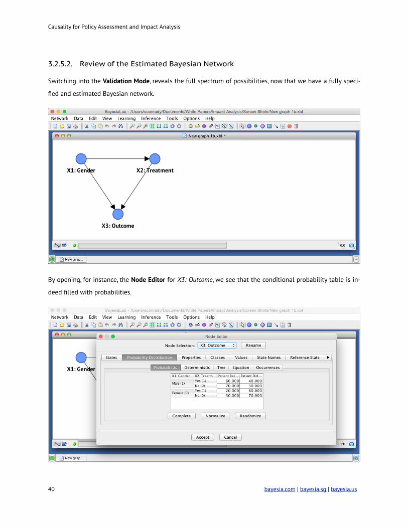
3.2.5.2. Review of the Estimated Bayesian Network

Switching into the Validation Mode, reveals the full spectrum of possibilities, now that we have a fully speci-

fied and estimated Bayesian network.

!

By opening, for instance, the Node Editor for X3: Outcome, we see that the conditional probability table is in-

deed filled with probabilities.

!






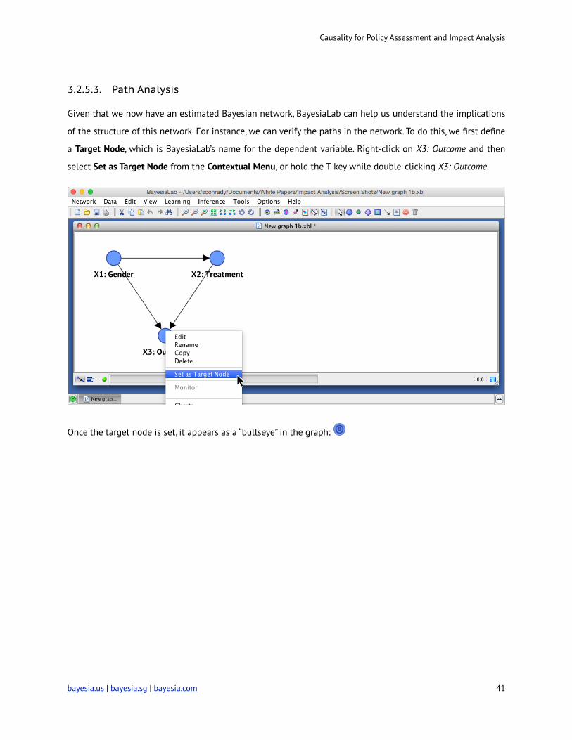
3.2.5.3. Path Analysis

Given that we now have an estimated Bayesian network, BayesiaLab can help us understand the implications

of the structure of this network. For instance, we can verify the paths in the network. To do this, we first define

a Target Node, which is BayesiaLab’s name for the dependent variable. Right-click on X3: Outcome and then

select Set as Target Node from the Contextual Menu, or hold the T-key while double-clicking X3: Outcome.

!

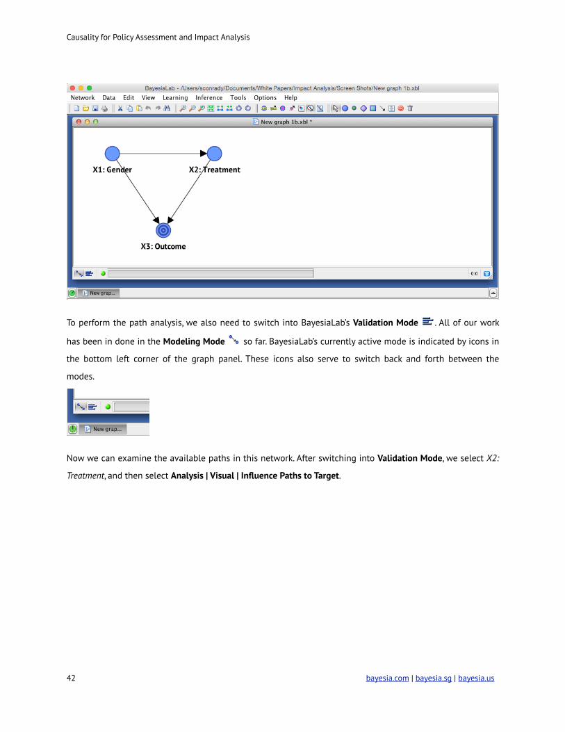
Once the target node is set, it appears as a “bullseye” in the graph: !






!

To perform the path analysis, we also need to switch into BayesiaLab’s Validation Mode ! . All of our work

has been in done in the Modeling Mode ! so far. BayesiaLab’s currently active mode is indicated by icons in

the bottom left corner of the graph panel. These icons also serve to switch back and forth between the

modes.

!

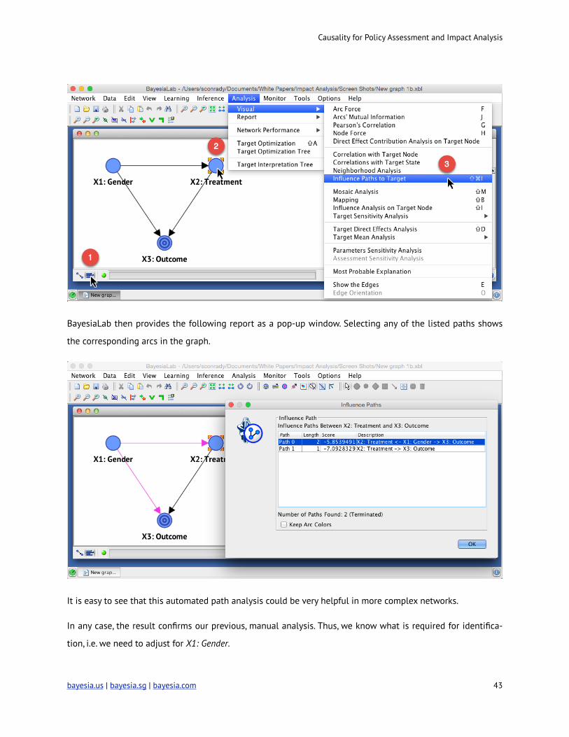
Now we can examine the available paths in this network. After switching into Validation Mode, we select X2:

Treatment, and then select Analysis | Visual | Influence Paths to Target.






!

BayesiaLab then provides the following report as a pop-up window. Selecting any of the listed paths shows

the corresponding arcs in the graph.

!

It is easy to see that this automated path analysis could be very helpful in more complex networks.

In any case, the result confirms our previous, manual analysis. Thus, we know what is required for identifica-

tion, i.e. we need to adjust for X1: Gender.






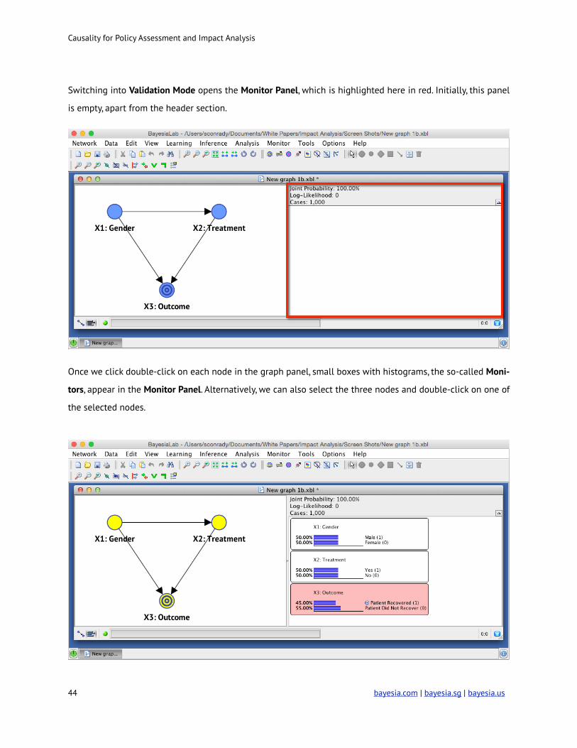
Switching into Validation Mode opens the Monitor Panel, which is highlighted here in red. Initially, this panel

is empty, apart from the header section.

!

Once we click double-click on each node in the graph panel, small boxes with histograms, the so-called Moni-

tors, appear in the Monitor Panel. Alternatively, we can also select the three nodes and double-click on one of

the selected nodes.






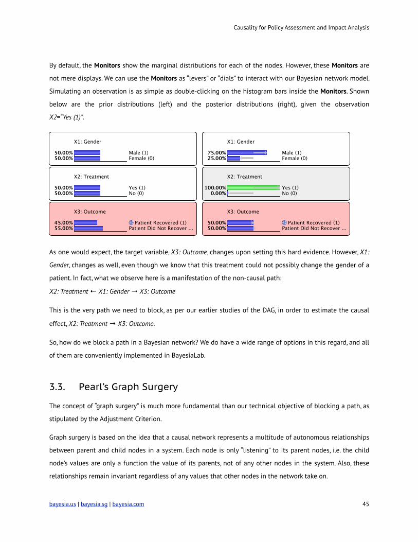
By default, the Monitors show the marginal distributions for each of the nodes. However, these Monitors are

not mere displays. We can use the Monitors as “levers” or “dials” to interact with our Bayesian network model.

Simulating an observation is as simple as double-clicking on the histogram bars inside the Monitors. Shown

below are the prior distributions (left) and the posterior distributions (right), given the observation

X2=“Yes (1)”.

! !

As one would expect, the target variable, X3: Outcome, changes upon setting this hard evidence. However, X1:

Gender, changes as well, even though we know that this treatment could not possibly change the gender of a

patient. In fact, what we observe here is a manifestation of the non-causal path:

X2: Treatment ← X1: Gender → X3: Outcome

This is the very path we need to block, as per our earlier studies of the DAG, in order to estimate the causal

effect, X2: Treatment → X3: Outcome.

So, how do we block a path in a Bayesian network? We do have a wide range of options in this regard, and all

of them are conveniently implemented in BayesiaLab.

3.3. Pearl’s Graph Surgery

The concept of “graph surgery” is much more fundamental than our technical objective of blocking a path, as

stipulated by the Adjustment Criterion.

Graph surgery is based on the idea that a causal network represents a multitude of autonomous relationships

between parent and child nodes in a system. Each node is only “listening” to its parent nodes, i.e. the child

node’s values are only a function the value of its parents, not of any other nodes in the system. Also, these

relationships remain invariant regardless of any values that other nodes in the network take on.






Should a node in this system be subjected to an outside intervention, the natural relationship between this

node and its parents would be severed. This node no longer naturally “obeys” inputs from its parent nodes;

rather an external force fixes the node to a new value, regardless of what the values of the parent nodes

would normally dictate. Despite this particular disruption, the other parts of the network remain unaffected in

their structure.

How does this help us estimate the causal effect? The idea is to consider the causal effect estimation as a

simulated intervention in the given system. Removing the arcs going into X2: Treatment implies that all the

non-causal paths between the X2 and the effect, X3, no longer exist, without blocking the causal path (i.e. the

same conditions apply as with the Adjustment Criterion).

Whereas previously, we computed the association in a system and interpreted it causally, we now have a

causal network as a computational device, i.e. the Bayesian network, and can simulate what happens upon

application of the cause. Applying the cause is the same as an intervention on a node in the network.

In our example, we wish to determine the effect of X2: Treatment, our cause, on X3: Outcome, the presumed

effect. In its natural state, X2: Treatment, is a function of its sole parent X1: Gender. To simulate the cause, we

must intervene on X2 and set it to specific values, i.e. “Yes (1)” or “No (0)”, regardless of what X1 would have

induced. This severs the inbound arc from X1 into X2, as if it were surgically removed. However, all other

properties remain unaffected, i.e. the distribution of X1, the arc between X1 and X3, and the arc between X2

and X3. This means, after performing the graph surgery, setting X2 to any value is an intervention, and any

effects must be causal.

While we could perform graph surgery manually on the given network, this function is automated in

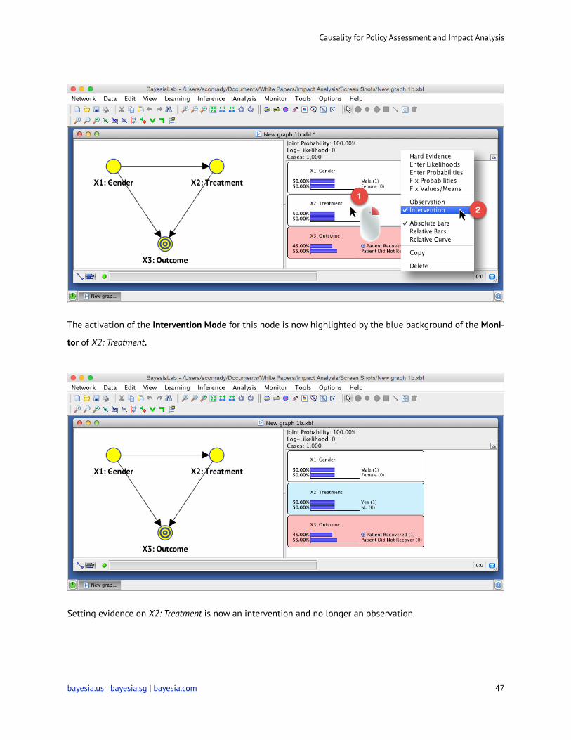
BayesiaLab. After right-clicking on the Monitor of the node X2: Treatment, we select Intervention from the

contextual menu.






!

The activation of the Intervention Mode for this node is now highlighted by the blue background of the Moni-

tor of X2: Treatment.

!

Setting evidence on X2: Treatment is now an intervention and no longer an observation.






!

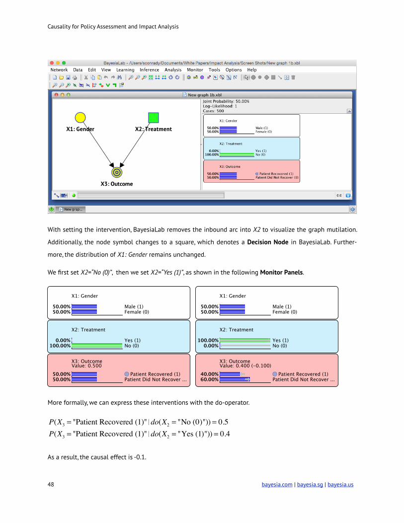
With setting the intervention, BayesiaLab removes the inbound arc into X2 to visualize the graph mutilation.

Additionally, the node symbol changes to a square, which denotes a Decision Node in BayesiaLab. Further-

more, the distribution of X1: Gender remains unchanged.

We first set X2=“No (0)”, then we set X2=“Yes (1)”, as shown in the following Monitor Panels.

! !

More formally, we can express these interventions with the do-operator.

!

As a result, the causal effect is -0.1.

P(X3 = "Patient Recovered (1)"�do(X2 = "No (0)")) = 0.5P(X3 = "Patient Recovered (1)"�do(X2 = "Yes (1)")) = 0.4






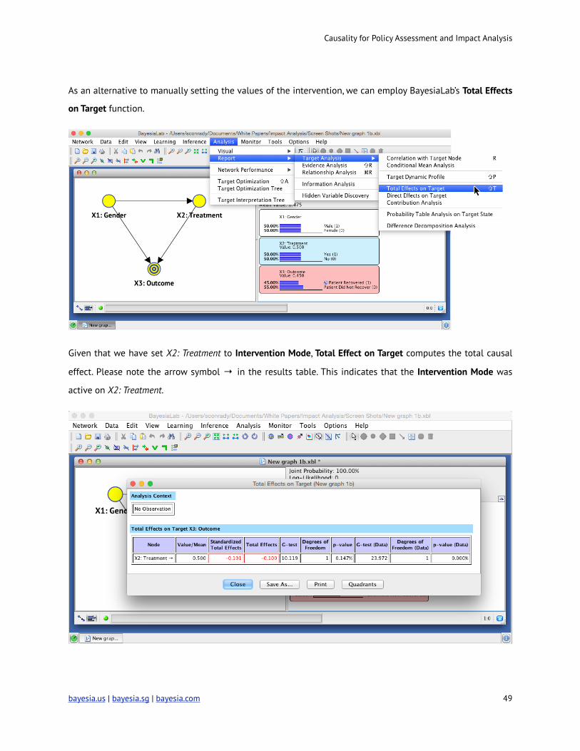
As an alternative to manually setting the values of the intervention, we can employ BayesiaLab’s Total Effects

on Target function.

!

Given that we have set X2: Treatment to Intervention Mode, Total Effect on Target computes the total causal

effect. Please note the arrow symbol → in the results table. This indicates that the Intervention Mode was

active on X2: Treatment.

!






3.4. Introduction to Matching

Earlier in this tutorial, adjustment was achieved by including the relevant variables in a regression. Instead,

we now perform adjustment by matching. In statistics, matching refers to the technique of making distribu-

tions of the sub-populations we are comparing, including multivariate distributions, as similar as possible to

each other. Applying matching to a variable qualifies as adjustment, and, as such, we can use it with the ob-

jective of keeping causal paths open and blocking non-causal paths.

In our example, matching is fairly simple as we only need to match a single binary variable, i.e. X1: Gender.

That will meet our requirement for adjustment and block the only non-causal path in our model.

3.4.1. Intuition for Matching

As the DAG-related terminology, e.g., “blocking paths”, may not be universally understood by a non-technical

audience, we can offer a more intuitive interpretation of matching, which our example can illustrate very well.

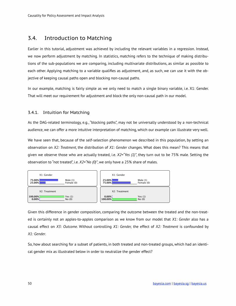
We have seen that, because of the self-selection phenomenon we described in this population, by setting an

observation on X2: Treatment, the distribution of X1: Gender changes. What does this mean? This means that

given we observe those who are actually treated, i.e. X2=“Yes (1)”, they turn out to be 75% male. Setting the

observation to “not treated”, i.e. X2=“No (0)”, we only have a 25% share of males.

! !

Given this difference in gender composition, comparing the outcome between the treated and the non-treat-

ed is certainly not an apples-to-apples comparison as we know from our model that X1: Gender also has a

causal effect on X3: Outcome. Without controlling X1: Gender, the effect of X2: Treatment is confounded by

X1: Gender.

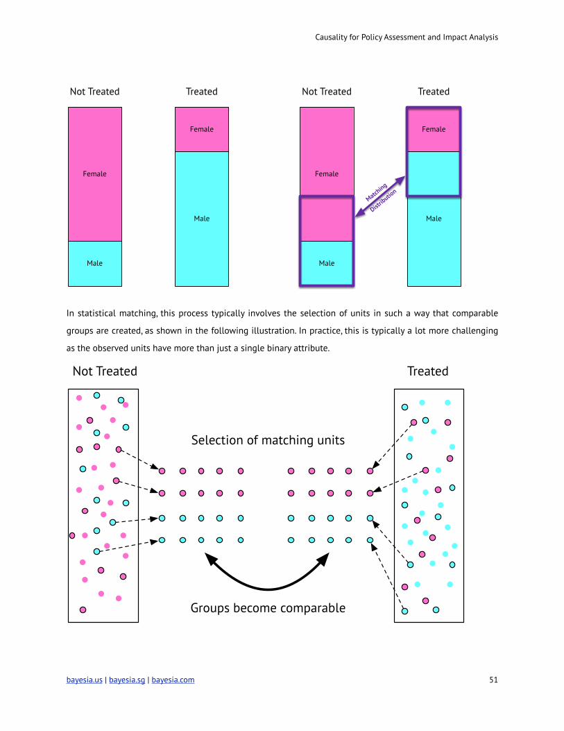
So, how about searching for a subset of patients, in both treated and non-treated groups, which had an identi-

cal gender mix as illustrated below in order to neutralize the gender effect?






!

In statistical matching, this process typically involves the selection of units in such a way that comparable

groups are created, as shown in the following illustration. In practice, this is typically a lot more challenging

as the observed units have more than just a single binary attribute.

!

Female

Male

Female

Male

TreatedNot Treated

Female

Male

Female

Male

TreatedNot Treated

Matching

Distribution

Not Treated Treated

Selection of matching units

Groups become comparable






This approach can be extended to higher dimensions, meaning that the observed units need to be matched

on a range of attributes, often including both continuous and discrete variables. In that case, exact matching

is rarely feasible, and some similarity measures must be utilized to define a “match.”

3.5. Jouffe’s Likelihood Matching

With Likelihood Matching, as it is implemented in BayesiaLab, however, we do not directly match the underly-

ing observations. Rather we match the distributions of the relevant nodes on the basis of the joint probability

distribution represented by the Bayesian network.

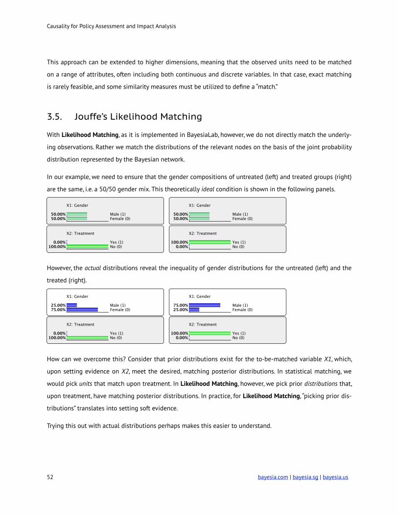
In our example, we need to ensure that the gender compositions of untreated (left) and treated groups (right)

are the same, i.e. a 50/50 gender mix. This theoretically ideal condition is shown in the following panels.

! !

However, the actual distributions reveal the inequality of gender distributions for the untreated (left) and the

treated (right).

! !

How can we overcome this? Consider that prior distributions exist for the to-be-matched variable X1, which,

upon setting evidence on X2, meet the desired, matching posterior distributions. In statistical matching, we

would pick units that match upon treatment. In Likelihood Matching, however, we pick prior distributions that,

upon treatment, have matching posterior distributions. In practice, for Likelihood Matching, “picking prior dis-

tributions” translates into setting soft evidence.

Trying this out with actual distributions perhaps makes this easier to understand.






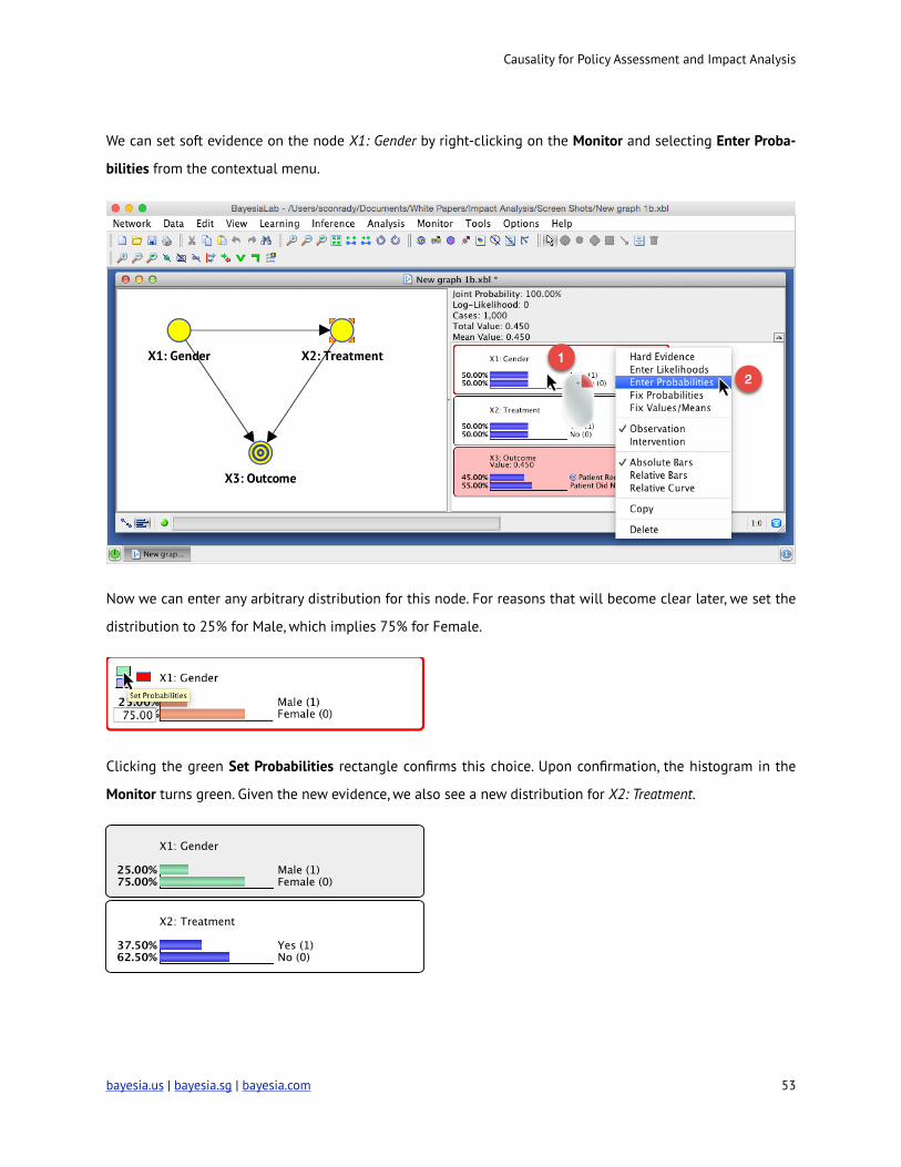
We can set soft evidence on the node X1: Gender by right-clicking on the Monitor and selecting Enter Proba-

bilities from the contextual menu.

!

Now we can enter any arbitrary distribution for this node. For reasons that will become clear later, we set the

distribution to 25% for Male, which implies 75% for Female.

!

Clicking the green Set Probabilities rectangle confirms this choice. Upon confirmation, the histogram in the

Monitor turns green. Given the new evidence, we also see a new distribution for X2: Treatment.

!






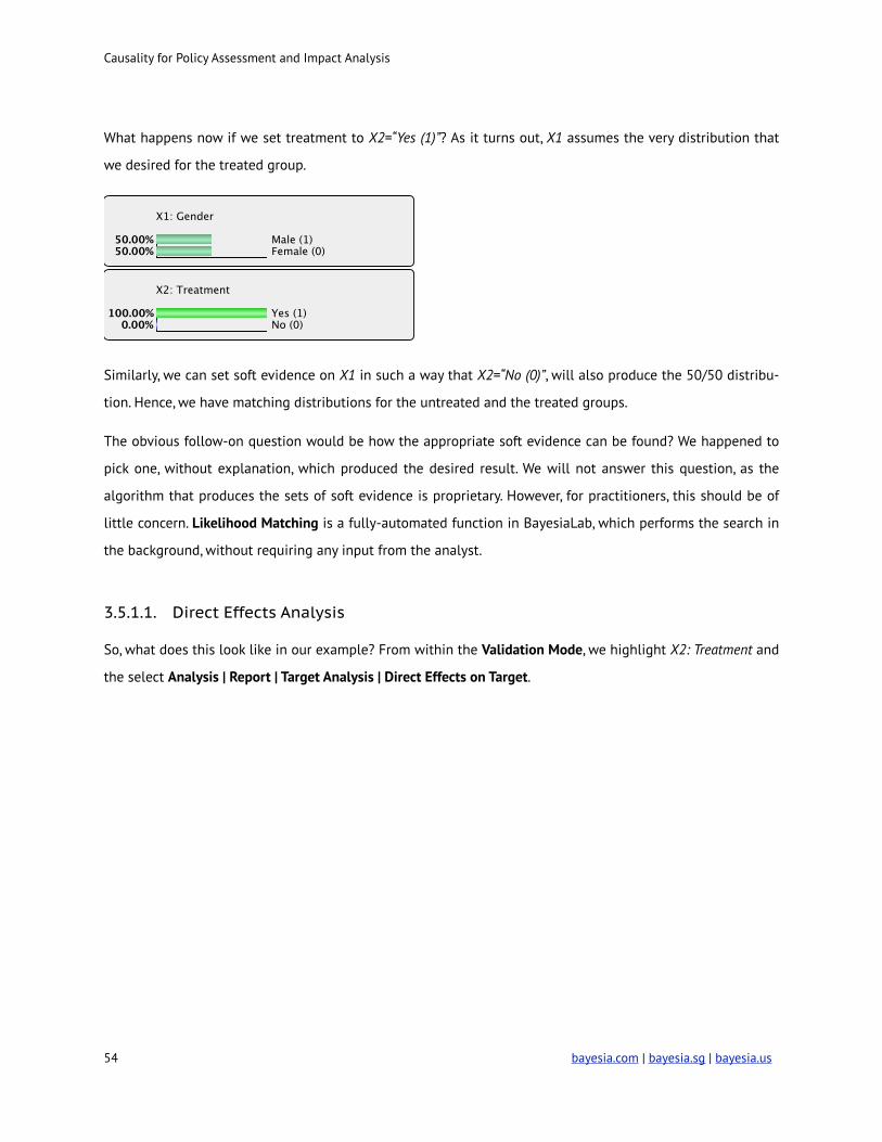
What happens now if we set treatment to X2=“Yes (1)”? As it turns out, X1 assumes the very distribution that

we desired for the treated group.

!

Similarly, we can set soft evidence on X1 in such a way that X2=“No (0)”, will also produce the 50/50 distribu-

tion. Hence, we have matching distributions for the untreated and the treated groups.

The obvious follow-on question would be how the appropriate soft evidence can be found? We happened to

pick one, without explanation, which produced the desired result. We will not answer this question, as the

algorithm that produces the sets of soft evidence is proprietary. However, for practitioners, this should be of

little concern. Likelihood Matching is a fully-automated function in BayesiaLab, which performs the search in

the background, without requiring any input from the analyst.

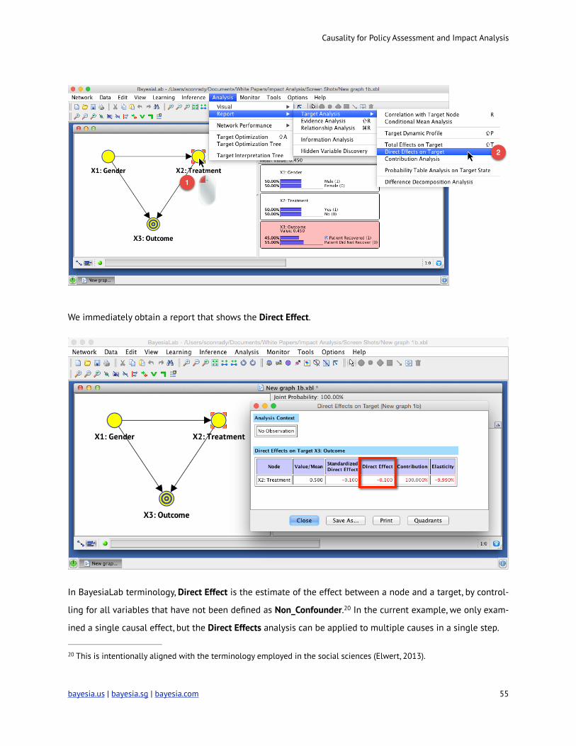
3.5.1.1. Direct Effects Analysis

So, what does this look like in our example? From within the Validation Mode, we highlight X2: Treatment and

the select Analysis | Report | Target Analysis | Direct Effects on Target.






!

We immediately obtain a report that shows the Direct Effect.

!

In BayesiaLab terminology, Direct Effect is the estimate of the effect between a node and a target, by control-

ling for all variables that have not been defined as Non_Confounder. In the current example, we only exam20 -

ined a single causal effect, but the Direct Effects analysis can be applied to multiple causes in a single step.

This is intentionally aligned with the terminology employed in the social sciences (Elwert, 2013).20






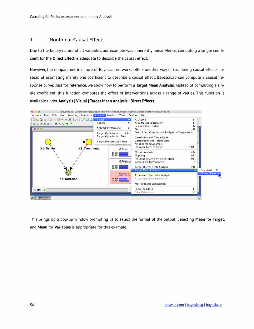
1. Nonlinear Causal Effects

Due to the binary nature of all variables, our example was inherently linear. Hence, computing a single coeffi-

cient for the Direct Effect is adequate to describe the causal effect.

However, the nonparametric nature of Bayesian networks offers another way of examining causal effects. In-

stead of estimating merely one coefficient to describe a causal effect, BayesiaLab can compute a causal “re-

sponse curve.” Just for reference, we show how to perform a Target Mean Analysis. Instead of computing a sin-

gle coefficient, this function computes the effect of interventions across a range of values. This function is

available under Analysis | Visual | Target Mean Analysis | Direct Effects.

!

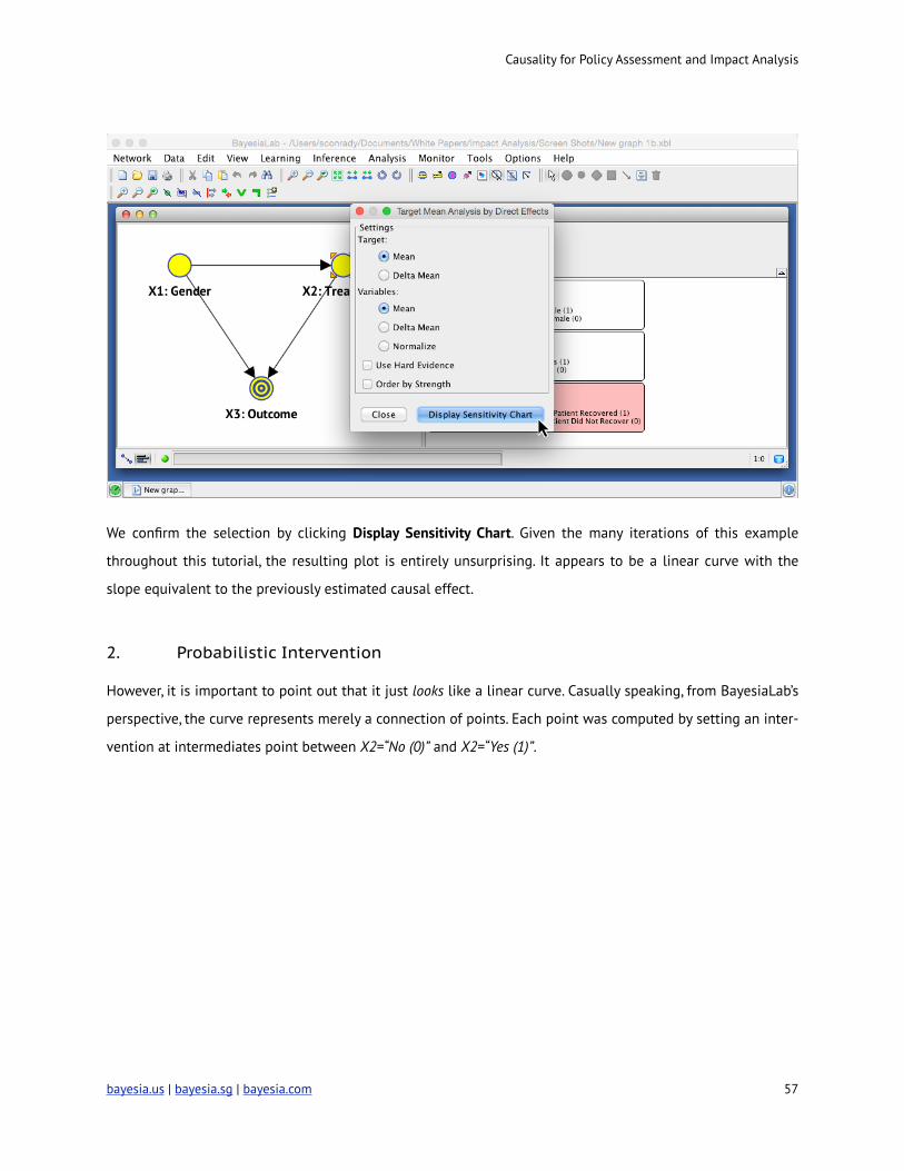
This brings up a pop-up window prompting us to select the format of the output. Selecting Mean for Target,

and Mean for Variables is appropriate for this example.






!

We confirm the selection by clicking Display Sensitivity Chart. Given the many iterations of this example

throughout this tutorial, the resulting plot is entirely unsurprising. It appears to be a linear curve with the

slope equivalent to the previously estimated causal effect.

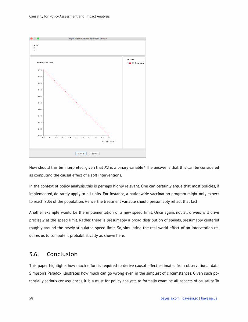
2. Probabilistic Intervention

However, it is important to point out that it just looks like a linear curve. Casually speaking, from BayesiaLab’s

perspective, the curve represents merely a connection of points. Each point was computed by setting an inter-

vention at intermediates point between X2=“No (0)” and X2=“Yes (1)”.






!

How should this be interpreted, given that X2 is a binary variable? The answer is that this can be considered

as computing the causal effect of a soft interventions.

In the context of policy analysis, this is perhaps highly relevant. One can certainly argue that most policies, if

implemented, do rarely apply to all units. For instance, a nationwide vaccination program might only expect

to reach 80% of the population. Hence, the treatment variable should presumably reflect that fact.

Another example would be the implementation of a new speed limit. Once again, not all drivers will drive

precisely at the speed limit. Rather, there is presumably a broad distribution of speeds, presumably centered

roughly around the newly-stipulated speed limit. So, simulating the real-world effect of an intervention re-

quires us to compute it probabilistically, as shown here.

3.6. Conclusion

This paper highlights how much effort is required to derive causal effect estimates from observational data.

Simpson’s Paradox illustrates how much can go wrong even in the simplest of circumstances. Given such po-

tentially serious consequences, it is a must for policy analysts to formally examine all aspects of causality. To






paraphrase Judea Pearl, we must not leave causal considerations to the mercy of intuition and good judge-

ment.

It is fortunate that causality has emerged from its pariah status in recent decades, which has allowed tremen-

dous progress in theoretical research and practical tools. “…practical problems relying on casual information

that long were regarded as either metaphysical or unmanageable can now be solved using elementary math-

ematics.” (Pearl, 1999)

Directed Acyclic Graphs, Bayesian networks, and the BayesiaLab software platform are the direct result of this

research progress. It is now upon the community of practitioners to embrace this progress to develop better

policies, for the benefit of all of us.






4. References Achen, Christopher H. Interpreting and Using Regression. Sage Publications, Inc, 1982.

Adelle, Camilla, and Sabine Weiland. “Policy Assessment: The State of the Art.” Impact Assessment and Project

Appraisal 30, no. 1 (March 1, 2012): 25–33. doi:10.1080/14615517.2012.663256.

Berk, Richard. “What You Can and Can’t Properly Do with Regression.” Journal of Quantitative Criminology 26,

no. 4 (2010): 481–87.

Brady, H.E. “Models of Causal Inference: Going beyond the Neyman-Rubin-Holland Theory.” In Annual Meeting

of the Midwest Political Science Association, Chicago, IL, 2002.

Cochran, William G., and Donald B. Rubin. “Controlling Bias in Observational Studies: A Review.” Sankhyā: The

Indian Journal of Statistics, Series A 35, no. 4 (December 1, 1973): 417–46.

Conrady, Stefan, and Lionel Jouffe. Paradoxes and Fallacies - Resolving Some Well-Known Puzzles with

Bayesian Networks. Bayesia USA, May 2, 2011. http://www.bayesia.us/paradoxes-and-fallacies.

Dehejia, Rajeev H., and Sadek Wahba. Causal Effects in Non-Experimental Studies: Re-Evaluating the Evalua-

tion of Training Programs. Working Paper. National Bureau of Economic Research, June 1998. http://

www.nber.org/papers/w6586.

Elwert, Felix. “Graphical Causal Models.” In Handbook of Causal Analysis for Social Research, edited by Stephen

L. Morgan. Handbooks of Sociology and Social Research. Dordrecht: Springer Netherlands, 2013. http://

link.springer.com/10.1007/978-94-007-6094-3.

Elwert, Felix, and Christopher Winship. “Endogenous Selection Bias: The Problem of Conditioning on a Collider

Variable.” Annual Review of Sociology 40, no. 1 (July 30, 2014): 31–53. doi:10.1146/annurev-

soc-071913-043455.

Gelman, Andrew, and Jennifer Hill. Data Analysis Using Regression and Multilevel/Hierarchical Models. 1st ed.

Cambridge University Press, 2006.

Gill, Judith I., and Laura Saunders. “Toward a Definition of Policy Analysis.” New Directions for Institutional Re-

search 1992, no. 76 (1992): 5–13. doi:10.1002/ir.37019927603.

Hagmayer, Y., S.A. Sloman, D.A. Lagnado, and M.R. Waldmann. “Causal Reasoning through Intervention.” Causal

Learning: Psychology, Philosophy, and Computation, 2007, 86–100.






Hagmayer, Y., and M. R Waldmann. “Simulating Causal Models: The Way to Structural Sensitivity.” In Proceed-

ings of the Twenty-Second Annual Conference of the Cognitive Science Society: August 13-15, 2000, In-

stitute for Research in Cognitive Science, University of Pennsylvania, Philadelphia, PA, 214, 2000.

Heckman, James, Hidehiko Ichimura, Jeffrey Smith, and Petra Todd. “Characterizing Selection Bias Using Exper-

imental Data.” Econometrica 66, no. 5 (1998): 1017–98. doi:10.2307/2999630.

Holland, Paul W. “Statistics and Causal Inference.” Journal of the American Statistical Association 81, no. 396

(1986): 945–60.

Hoover, Kevin D. Counterfactuals and Causal Structure. SSRN Scholarly Paper. Rochester, NY: Social Science

Research Network, September 23, 2009. http://papers.ssrn.com/abstract=1477531.

Imai, Kosuke, Luke Keele, Dustin Tingley, and Teppei Yamamoto. “Unpacking the Black Box of Causality: Learn-

ing about Causal Mechanisms from Experimental and Observational Studies.” American Political Science

Review 105, no. 04 (November 2011): 765–89. doi:10.1017/S0003055411000414.

Imbens, G. “Estimating Average Treatment Effects in Stata.” In West Coast Stata Users’ Group Meetings 2007,

2007.

“International Association for Impact Assessment.” Accessed October 19, 2014. http://www.iaia.org/about/.

Johnson, Jeff W. “A Heuristic Method for Estimating the Relative Weight of Predictor Variables in Multiple Re-

gression.” Multivariate Behavioral Research 35, no. 1 (January 2000): 1–19. doi:10.1207/S15327906M-

BR3501_1.

Manski, Charles F. Identification Problems in the Social Sciences. Harvard University Press, 1999.

Morgan, Stephen L., and Christopher Winship. Counterfactuals and Causal Inference: Methods and Principles

for Social Research. 1st ed. Cambridge University Press, 2007.

Pearl, J., and S. Russell. “Bayesian Networks.” Handbook of Brain Theory and Neural Networks, Ed. M. Arbib. MIT

Press.[DAL], 2001.

Pearl, Judea. Causality: Models, Reasoning and Inference. 2nd ed. Cambridge University Press, 2009.

———. “Statistics, Causality, and Graphs.” In Causal Models and Intelligent Data Management, 3–16. Springer,

1999. http://link.springer.com/chapter/10.1007/978-3-642-58648-4_1.

Rosenbaum, Paul R. Observational Studies. Softcover reprint of hardcover 2nd ed. 2002. Springer, 2010.






Rosenbaum, Paul R., and Donald B. Rubin. “The Central Role of the Propensity Score in Observational Studies

for Causal Effects.” Biometrika 70, no. 1 (April 1, 1983): 41–55. doi:10.1093/biomet/70.1.41.

Rubin, Donald B. “Estimating Causal Effects of Treatments in Randomized and Nonrandomized Studies.” Jour-

nal of Educational Psychology 66, no. 5 (1974): 688–701. doi:10.1037/h0037350.

———. Matched Sampling for Causal Effects. 1st ed. Cambridge University Press, 2006.

Sekhon, J.S. The Neyman-Rubin Model of Causal Inference and Estimation via Matching Methods. Oxford: Ox-

ford University Press, 2008.

Shmueli, Galit. “To Explain or to Predict?” Statistical Science 25, no. 3 (August 2010): 289–310. doi:

10.1214/10-STS330.

Stolley, Paul D. “When Genius Errs: R. A. Fisher and the Lung Cancer Controversy.” American Journal of Epidemi-

ology 133, no. 5 (March 1, 1991): 416–25.

Stressor Identification Guidance Document. Washington, DC: U.S Environmental Protection Agency, December

2000.

Stuart, E.A., and D.B. Rubin. “Matching Methods for Causal Inference: Designing Observational Studies.” Har-

vard University Department of Statistics Mimeo, 2004.

Tuna, Cari. “When Combined Data Reveal the Flaw of Averages.” Wall Street Journal, December 2, 2009, sec. US.

http://online.wsj.com/articles/SB125970744553071829.

U.S. Environmental Protection Agency. “CADDIS Home Page.” Data & Tools. Accessed October 16, 2014. http://

www.epa.gov/caddis/.

———. “EPA - TTN - ECAS - Regulatory Impact Analyses.” Regulatory Impact Analyses, September 9, 2014. http://

www.epa.gov/ttnecas1/ria.html.






5. Contact Information

Bayesia USA

312 Hamlet’s End Way

Franklin, TN 37067

USA

Phone: +1 888-386-8383

[email protected]

www.bayesia.us

Bayesia Singapore Pte. Ltd.

28 Maxwell Road

#03-05, Red Dot Traffic

Singapore 069120

Phone: +65 3158 2690

[email protected]

www.bayesia.sg

Bayesia S.A.S.

6, rue Léonard de Vinci

BP 119

53001 Laval Cedex

France

Phone: +33(0)2 43 49 75 69

[email protected]

www.bayesia.com

Copyright

© 2014 Bayesia USA, Bayesia S.A.S. and Bayesia Singapore Pte. Ltd. All rights reserved.











impact analysis v12

Documents

policy assessment

causal identification

policy analysis

causal inference

impact analysis1

impact assessments

causal questions

effect estimation