impact and implications of climate variability and change

Impact and implications of climatevariability and change on glacier mass

balance in Kenya

University of Reading

Department of Mathematics, Meteorology and Physics.

Neeral Shah

A dissertation submitted in partial fulfilment of the requirement for the

degree of MSc in Mathematical and Numerical Modelling of the

Atmosphere and Ocean

Declaration

I confirm that this is my own work and the use of all material from other

sources has been properly and fully acknowledged.

Neeral Shah

ii

Abstract

Kenya’s economy relies heavily on the agricultural indsutry as its main

source of economy. Glaciers provide a large store of freshwater and mod-

elling of the meltwater associated with this is of great interest to water

management. with growing concern over the impact of glacier retreat on

runoff and streamflow, this study aims to simulate runoff from the tropical

Lewis Glacier in Central Kenya and its impacts on runoff due to climate

variability.

Acknowledgments

The writing of this dissertation has been one of the most significant academic

challenges I have ever had to face. Without the support, patience and

guidance of the following people, this study would not have been completed.

It is to them I owe everlasting gratitude.

• To Professor Nigel Arnell, thank you for undertaking the role of be-

ing my supervisor and the duties associated with it. I have enjoyed

working with you.

• To the Mathematics and Meteorology departments at the University

of Reading, without whom this study would not have been possible.

Special thanks goes to Professor Mike Baines and Sue Davis for always

being there and giving a word or two of encouragement to keep us

going.

• To Mr Simon Gosling, thank you for all the data sets you provided me

without which this project would not have been possible and the open

door policy you shared.

• To Rashmita and Jayendra Shah, you mean the world to me. Thank

you for supporting me and believing in all my endeavours.

• To Ankeet Shah, thank you for being my one of my sources of inspi-

ration.

• To Jasdeep Giddie, thank you for all your love and patience, for be-

lieving in me and most of all, for all the compromises you have had to

make this year so I could undertake this task.

i

ii

‘Asante Sana’ to all friends and family who have taken this journey with

me.

Contents

Acknowledgements i

1 Introduction 1

1.1 Background . . . . . . . . . . . . . . . . . . . . . . . . . . . . 1

1.2 Goals . . . . . . . . . . . . . . . . . . . . . . . . . . . . . . . 3

1.3 Outline . . . . . . . . . . . . . . . . . . . . . . . . . . . . . . 3

2 Experimental Design 4

2.1 The Study Approach . . . . . . . . . . . . . . . . . . . . . . . 4

2.2 The Lewis Glacier Model . . . . . . . . . . . . . . . . . . . . 5

2.3 The Hydrological Model - Mac-PDM . . . . . . . . . . . . . . 6

2.4 Emission Scenarios Data Sets . . . . . . . . . . . . . . . . . . 10

3 The Lewis Glacier Model 11

3.1 Background . . . . . . . . . . . . . . . . . . . . . . . . . . . . 11

3.2 Some Definitions . . . . . . . . . . . . . . . . . . . . . . . . . 12

3.3 The Model . . . . . . . . . . . . . . . . . . . . . . . . . . . . 13

3.4 Stability and Accuracy . . . . . . . . . . . . . . . . . . . . . . 17

4 Results and Analyses 19

4.1 Modelled Mass Balance Profile of the Lewis Glacier . . . . . . 19

iii

CONTENTS iv

4.2 Mass Balance and Volume of Glacier . . . . . . . . . . . . . . 20

4.3 Implications of Surface Runoff and Glacier Melt . . . . . . . . 20

4.4 Climate variability and Runoff . . . . . . . . . . . . . . . . . 21

5 Discussion and Summary 31

5.1 Caveats . . . . . . . . . . . . . . . . . . . . . . . . . . . . . . 31

5.2 Conclusion . . . . . . . . . . . . . . . . . . . . . . . . . . . . 32

5.3 Further Work . . . . . . . . . . . . . . . . . . . . . . . . . . . 33

Bibliography 33

Chapter 1

Introduction

1.1 Background

Kenya relies heavily on its natural resources to generate income. High alti-

tude, fertile soils and abundance of precipitation (1000mm) in Central and

Western Kenya make it the ideal place for growing tea and coffee, two of

Kenya’s highest GDP earners. Other agricultural goods such as horticulture

and sugar cane also rely heavily on water availability. The impacts on water

resources in Kenya due to climate variability are thus of great importance.

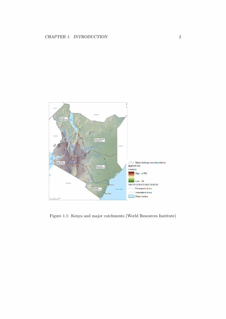
Mount Kenya is located on the equator in East Africa with the two

highest peaks, Batian and Nelion, reaching about 5,200 m. It lies at the

apex of three water sheds, Uasin Nyiro, Tana and Rift Valley catchments

as per the map below. According to Young & Hastenrath (1991), there are

total of 11 glaciers on Mount Kenya, of which the Lewis and Tyndall glaciers

are the two largest and most studied. In this study, the focus will be on the

modelling of the mass balance of the Lewis Glacier as it covers the largest

area of 0.31 km2.

In high mountainous catchments, glaciers represent the most important

water storage reservoir. Thus glacier mass balance estimated over long peri-

ods of time is a good indicator of the overall water balance of the catchment

(Schaefli et al. (2005)). The idea of mass balance is an important link be-

tween climatic inputs and and glacier behaviour and as a result future water

1

CHAPTER 1. INTRODUCTION 2

Figure 1.1: Kenya and major catchments (World Resources Institute)

CHAPTER 1. INTRODUCTION 3

balance can be predicted for catchments containing advancing or retreating

glaciers (Bienn and Evans (1998)).

1.2 Goals

The aims of this study are:

1. To model the mass balance profile of the Lewis Glacier using baseline

and climate change data; and

2. To assess the effects of the change in glacier mass balance on down-

stream water resources

1.3 Outline

The outline of the dissertation is as follows:

In the second chapter the study approach, an introduction to the glacier

model, the hydrological model and data sets used are discussed.

In Chapter 3, the glacier model based on Kaser (2001) and Kaser and

Osmaston (2002) is developed.

Results of the study are presented in Chapter 4.

Finally, Chapter 5 summarises the findings of the study along with

caveats and further work is proposed.

Chapter 2

Experimental Design

This is the chapter where I describe the models and data sets used.

1. Glacier model

2. Mac-PDM model

3. Data Basis

2.1 The Study Approach

The approach to the study on the effects of the Lewis Glacier on the hydro-

logical system in Kenya was as follows:

1. Develop a mass balance profile to evaluate the amount of water (and

hence runoff) held on the Lewis Glacier, Mount Kenya using baseline

and climatic data;

2. Convert mass balance into runoff by determining the volume of the

glacier and hence meltwater;

3. Compare the performance of the system between baseline and altered

climate inputs and between mass balance profiles and non mass bal-

ance profiles with baseline and altered climate inputs.

4

CHAPTER 2. EXPERIMENTAL DESIGN 5

4. Run the ‘Mac-PDM’ global hydrological model to simulate streamflow

in Kenya with baseline and climatic data;

5. Compare simulated runoff from the glacier and hydrological models

and note any impacts the glacier retreat may have on the catchment.

2.2 The Lewis Glacier Model

Glaciers account for 75% of the world’s fresh water. Of these, the tropics

account for 0.15% of global glacier area and hence freshwater sources.

Glaciers are an important part of the hydrological cycle as they act as

an intermediate store, regulating the seasonal and long-term runoff varia-

tions on the highest of mountain ranges (Kaser et al. (2003)). In addition,

mountainous regions are good sources of water suppply as they enhance

convective precipitation due to their orographic features.

Hydrological models that are able to simulate runoff from snow and ice

melt affected catchments are particularly useful to predict floods due to

sudden release of meltwater, water flow rate for hydro power dams located

in mountainous regiopns, and sources of freshwater supply for domestic,

agricultural and industrial purposes.

The modelling of the Lewis Glacier is based on calculation of the mass

balance using the vertical profile of specific mass balance (VBP) method

proposed by Kaser (2001)and Kaser and Osmaston (2002) which shall be

discussed in more detail in Chapter 3. This method involves seeking the

vertical mass blance gradient (variation of the mass budget with altitude)

in consideration of the vertical gradients of accumulation, air temperature,

albedo, the duration of the ablation period and a factor for the ratio between

melting and sublimation of the glacier.

The Glacier Model and the Hydrological Model

The glacier model outlined above is used to calculate the specific mass bal-

ance profile of a defined glacier in [kg m−2] in terms of its vertical accumula-


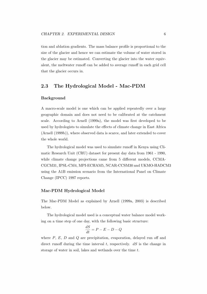
tion and ablation gradients. The mass balance profile is proportional to the

size of the glacier and hence we can estimate the volume of water stored in

the glacier may be estimated. Converting the glacier into the water equiv-

alent, the meltwater runoff can be added to average runoff in each grid cell

that the glacier occurs in.

2.3 The Hydrological Model - Mac-PDM

Background

A macro-scale model is one which can be applied repeatedly over a large

geographic domain and does not need to be calibrated at the catchment

scale. According to Arnell (1999a), the model was first developed to be

used by hydrologists to simulate the effects of climate change in East Africa

(Arnell (1999b)), where observed data is scarce, and later extended to cover

the whole world.

The hydrological model was used to simulate runoff in Kenya using Cli-

matic Research Unit (CRU) dataset for present day data from 1961 - 1990,

while climate change projections came from 5 different models, CCMA-

CGCM31, IPSL-CM4, MPI-ECHAM5, NCAR-CCSM30 and UKMO-HADCM3

using the A1B emission scenario from the International Panel on Climate

Change (IPCC) 1997 reports.

Mac-PDM Hydrological Model

The Mac-PDM Model as explained by Arnell (1999a, 2003) is described

below.

The hydrological model used is a conceptual water balance model work-

ing on a time step of one day, with the following basic structure:dS

dt= P − E −D −Q

where P , E, D and Q are precipitation, evaporation, delayed run off and

direct runoff during the time interval t, respectively. dS is the change in

storage of water in soil, lakes and wetlands over the time t.


Streamflow is simulated at a spatial resolution of 0.5 x 0.5◦ (or 2000 km2),

treating each grid cell as an independent catchment. Input parameters are

assumed to be constant across the entire grid cell while soil mositure stor-

age capacity varies with a statistical distribution across the grid cell. The

model parameters have not been calibrated from site data, but the perfor-

mance of the model has been validated and found that it simulates average

annual runoff reasonably well (Arnell, 1999a, 2003). The hydrological model

currently does not simulate melt water from glacierized areas.

The model differentiates precipitation as snow if temperature is below a

defined threshold and rain otherwise. Snow melts once temperature reaches

another threshold. Precipitation is intercepted by vegetation until the in-

terception capacity has been reached, the excess falling to the ground. Pre-

cipitation that has not been intercepted or on the ground is evaporated.

Potential evaporation is calculated using the Penman-Monteith formula:

E =1000λρw

[∆Rn + 86.4ρacp (es − e) /ra

∆ + γ [1 + rs/ra]

]where λ is the latent heat of vapourisation, ρw is density of water, ρa is

density of air, ∆ is gradient of the relationship between vapour pressure and

temperature, Rn is net radiation, cp is specific heat capacity of the air, esis saturated vapour pressure, e is vapour pressure, ra is aerodynamic re-

sistance, rs is surface resistance and γ, is the psychometric constant. The

aerodynamic resistance and surface resistance are dependent on vegetation

type and thus each grid cell is divided into either ’grass’ or ’not grass’ veg-

etation type. Characterisitics of ’not grass’ vary from cell to cell based on

the land cover data taken from the global land cover data set produced by

deFries et al. (1998). Each part of the cell has the same inputs and soil

properties and the output of the two parts is summed to give a total cell

response.

If the soil is saturated, water that reaches the ground becomes ’quick-

flow’, and infiltrates the soil otherwise. Soil moisture is depleted by evapo-

ration and drainage to a deep store (’slowflow’) when soil moisture storage

is above field capacity. A variable proportion of the grid cell is saturated at

any one time generating ’quickflow’ from this proportion of the cell. This is


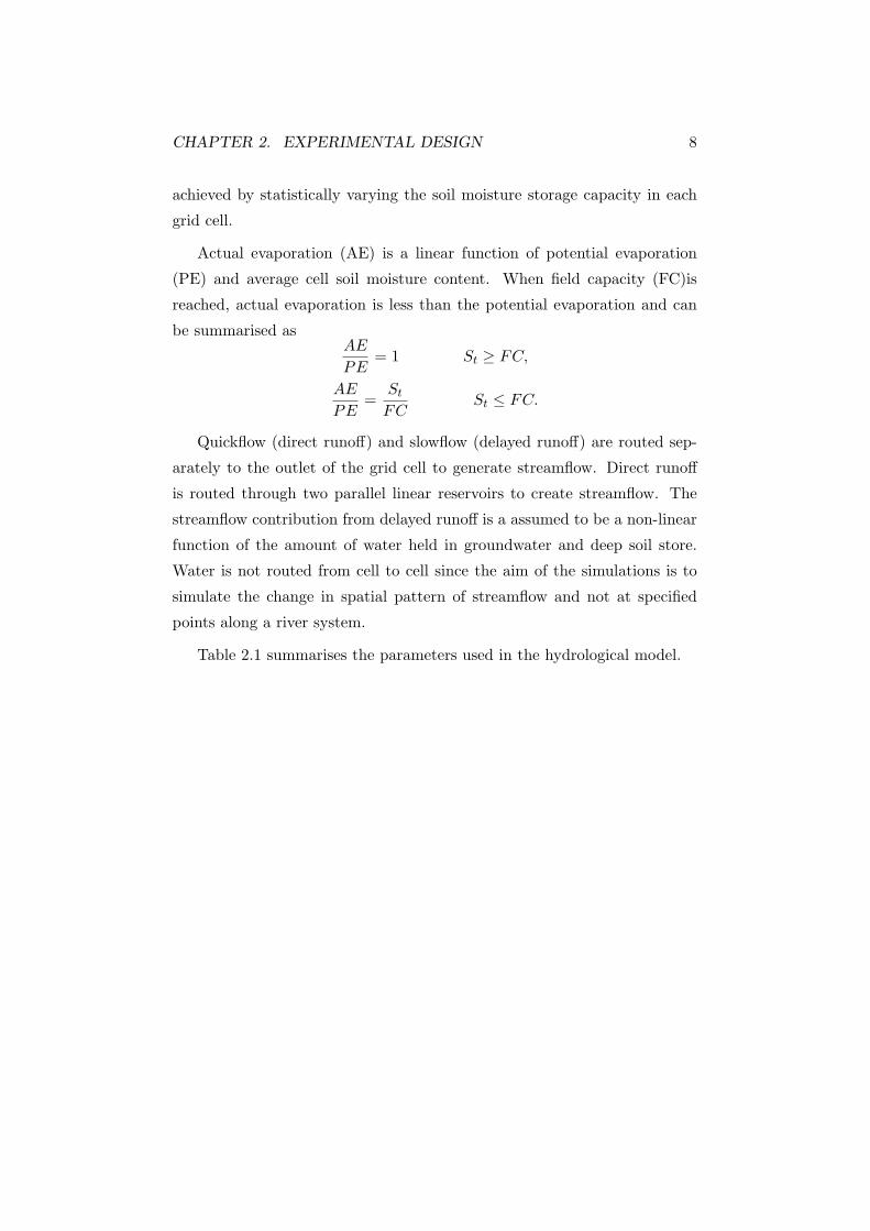
achieved by statistically varying the soil moisture storage capacity in each

grid cell.

Actual evaporation (AE) is a linear function of potential evaporation

(PE) and average cell soil moisture content. When field capacity (FC)is

reached, actual evaporation is less than the potential evaporation and can

be summarised asAE

PE= 1 St ≥ FC,

AE

PE=

St

FCSt ≤ FC.

Quickflow (direct runoff) and slowflow (delayed runoff) are routed sep-

arately to the outlet of the grid cell to generate streamflow. Direct runoff

is routed through two parallel linear reservoirs to create streamflow. The

streamflow contribution from delayed runoff is a assumed to be a non-linear

function of the amount of water held in groundwater and deep soil store.

Water is not routed from cell to cell since the aim of the simulations is to

simulate the change in spatial pattern of streamflow and not at specified

points along a river system.

Table 2.1 summarises the parameters used in the hydrological model.


Parameter Description Source

Tcrit Temperature threshold for snowfall and

snowmelt

0◦ C - Fixed

Melt Melt rate 4 mm ◦C−1 d−1) Fixed

b Parameter describing distribution of

soil moisture capacity

0.25 Fixed

Sat Saturation capacity in % Function of soil texture and vegeta-

tion

FC Field capacity in % Function of soil texture and vegeta-

tion

RFF fraction of cell that is not ”not grass” Function of vegetation type

γ Interception capacity Function of vegetation type

δ Parameters of interception model Fixed

Root depth Depth of vegetation used to define sat-

uration and field capacity in absolute

terms

Function of vegetation type

LAI Leaf area index used in Penman-

Monteith


rs Stomatal conductance used in Penman-

Monteith


Hc Vegetational roughness height used in

Penman-Monteith


Srout Routing parameter for direct runoff Fixed

Grout Routing parameter for delayed runoff Fixed

Each grid cell is classified according to a soil type based on United Na-

tions Food and Agriculture (FOA) data. Soil type is important as soil

moisture storage is a function of texture.

To account for variations in seasons, a sine curve is fitted to maximum

and minimum monthly temperatures with an additional random deviation

of 2◦ around the sine curve to simulate fluctuations in daily temperature.


2.4 Emission Scenarios Data Sets

The climate change data is based upon the pattern scaling technique. The

scenarios have been developed using ClimGen. The data for 5 GCMs, for

the A1B emissions scenario, for 2040-2069. The scenarios used are for the

patterns of climate change associated with 5 different General Circulation

Models (GCM). The 5 models are (modelling institution and model version):

• IPSL CM4

• CCCMA CGCM31

• UKMO HadCM3

• MPI ECHAM5

• NCAR CCSM30

The A1B scenario family describes a future world of very rapid economic

growth, global population that peaks in mid-century and declines thereafter,

and the rapid introduction of new and more efficient technologies. Major

underlying themes are convergence among regions, capacity building and

increased cultural and social interactions, with a substantial reduction in

regional differences in per capita income. The A1 scenario family develops

into three groups that describe alternative directions of technological change

in the energy system. The three A1 groups are distinguished by their techno-

logical emphasis: fossil intensive (A1FI), non-fossil energy sources (A1T), or

a balance across all sources (A1B) (where balanced is defined as not relying

too heavily on one particular energy source, on the assumption that simi-

lar improvement rates apply to all energy supply and end-use technologies)

(UNEP, 2001)

Chapter 3

The Lewis Glacier Model

3.1 Background

Modelling of glaciers (prediction of meltwater driven streamflow)has been

regarded as a valuable tool for efficient water resource management. As

a result, several models have been developed. According to Hock (2005),

the range of models used to forecast meltwater production from glaciers

ranges from energy-balance models to temperature-index models and several

mixtures of the two.

Glaciers can be classed into three broad categories, each with unique

characteristics: polar glaciers, midlatitude glaciers and tropical glaciers.

Tropical glaciers can be further divided into inner tropics and outer tropics

(Kaser and Osmaston, 2002).

Tropical glaciers have gained increased attention in the context of global

change due to their role in regional water budgets (Hastenrath, 1995). Glaciers

still exist near the Equator in Africa (Mount Kilimanjaro,Mount Kenya,

Ruwenzori Moutnains), South America (South America Andes) and New

Guinea (Irian Jaya), but have begun to retreat rapidly since the 19th cen-

tury.

According to Innes (2009) the limits of the tropics are defined where

1. the sun is directly overhead at some point in the year (23◦ N - 23◦);

11

CHAPTER 3. THE LEWIS GLACIER MODEL 12

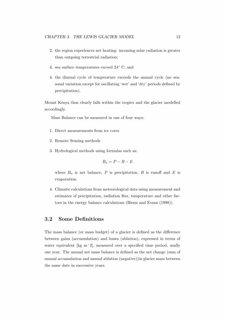
2. the region experiences net heating: incoming solar radiation is greater

than outgoing terrestrial radiation;

3. sea surface temperatures exceed 24◦ C; and

4. the diurnal cycle of temperature exceeds the annual cycle (no sea-

sonal variation except for oscillating ‘wet’ and ‘dry’ periods defined by

precipitation).

Mount Kenya thus clearly falls within the tropics and the glacier modelled

accordingly.

Mass Balance can be measured in one of four ways:

1. Direct measurements from ice cores

2. Remote Sensing methods

3. Hydrological methods using formulas such as:

Bn = P −R− E

where Bn is net balance, P is precipitation, R is runoff and E is

evaporation.

4. Climatic calculations from meteorological data using measurement and

estimates of precipitation, radiation flux, temperature and other fac-

tors in the energy balance calculations (Bienn and Evans (1998)).

3.2 Some Definitions

The mass balance (or mass budget) of a glacier is defined as the difference

between gains (accumulation) and losses (ablation), expressed in terms of

water equivalent [kg m−2], measured over a specified time period, usally

one year. The annual net mass balance is defined as the net change (sum of

annual accumulation and annual ablation (negative))in glacier mass between

the same date in successive years.


The amount of annual ablation and accumulation varies systematically

with altitude. The rate at which annual ablation and accumulation change

with altitude are termed ablation gradient and accumulation gradient, re-

spectively. Together they define the mass balance gradient.

Mass balance gradients link climatic conditions on ablation and accu-

mulation with glacier behaviour and is therefore an important measure of

glacier activity (Bienn and Evans, 1998). Ablation gradients vary approx-

imately linearly with altitude, being highest at the snout and decreasing

with altitude because temperature declines with higher altitude at a lapse

rate of 0.0065 K m−1. Conversely, accumulation generally increases with

altitude, rising from zero at the equilibrium line (ELA). ELA is the altitude

at which ablation is equal to accumulation and hence net mass balance is

zero. According to Kaser (2001) and Kaser and Osmaston (2002), the ELA

is more or less equal to the altitide at which the air temperature is 0◦ C at

the inner tropics.

3.3 The Model

The model described below is based on the vertical mass balance gradient

compiled by Kuhn (1980) and further developed by Kaser (2001) and Kaser

and Osmaston (2002).

The specific mass budget b at any altitude z on a glacier over a specific

period, usually one year, is made up of the sum of specific accumulation c(z)

and specific ablation a(z)

b(z) = c(z) + a(z). (3.1)

This is also true for the vertical mass balance gradient

db

dz=∂c

∂z+∂a

∂z(3.2)

with c(z) positive, a(z) negative and z positive vertically upward.

Ablation is made up of meltwater runoff m(z) and the sublimation pro-

cess s(z) into the atmosphere, Both are goverened by latent heat fluxes

QM (z) for melting and QL(z) for sublimation. Thus specific ablation is


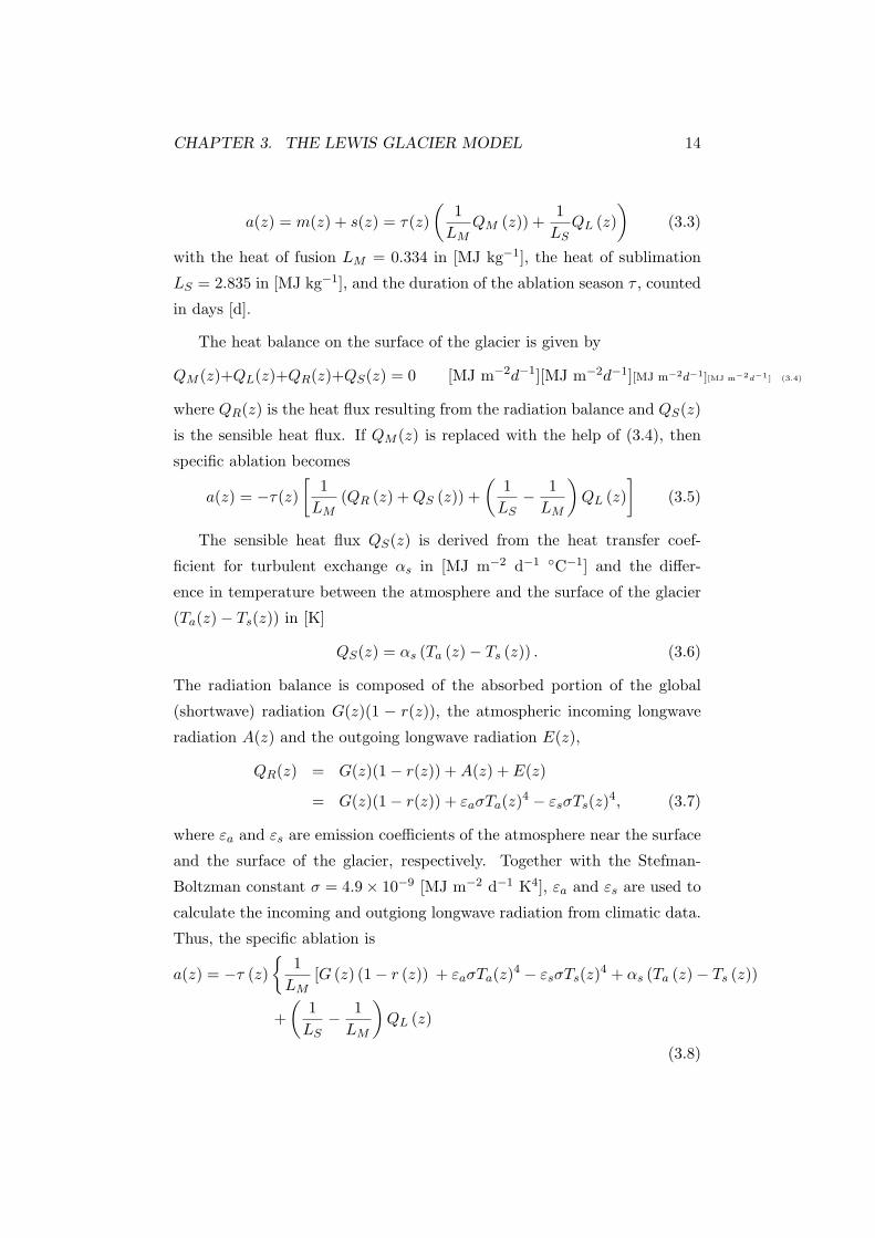
a(z) = m(z) + s(z) = τ(z)(

1LM

QM (z)) +1LS

QL (z))

(3.3)

with the heat of fusion LM = 0.334 in [MJ kg−1], the heat of sublimation

LS = 2.835 in [MJ kg−1], and the duration of the ablation season τ , counted

in days [d].

The heat balance on the surface of the glacier is given by

QM (z)+QL(z)+QR(z)+QS(z) = 0 [MJ m−2d−1][MJ m−2d−1][MJ m−2d−1][MJ m−2d−1] (3.4)

where QR(z) is the heat flux resulting from the radiation balance and QS(z)

is the sensible heat flux. If QM (z) is replaced with the help of (3.4), then

specific ablation becomes

a(z) = −τ(z)[

1LM

(QR (z) +QS (z)) +(

1LS− 1LM

)QL (z)

](3.5)

The sensible heat flux QS(z) is derived from the heat transfer coef-

ficient for turbulent exchange αs in [MJ m−2 d−1 ◦C−1] and the differ-

ence in temperature between the atmosphere and the surface of the glacier

(Ta(z)− Ts(z)) in [K]

QS(z) = αs (Ta (z)− Ts (z)) . (3.6)

The radiation balance is composed of the absorbed portion of the global

(shortwave) radiation G(z)(1 − r(z)), the atmospheric incoming longwave

radiation A(z) and the outgoing longwave radiation E(z),

QR(z) = G(z)(1− r(z)) +A(z) + E(z)

= G(z)(1− r(z)) + εaσTa(z)4 − εsσTs(z)4, (3.7)

where εa and εs are emission coefficients of the atmosphere near the surface

and the surface of the glacier, respectively. Together with the Stefman-

Boltzman constant σ = 4.9× 10−9 [MJ m−2 d−1 K4], εa and εs are used to

calculate the incoming and outgiong longwave radiation from climatic data.

Thus, the specific ablation is

a(z) = −τ (z){

1LM

[G (z) (1− r (z)) + εaσTa(z)4 − εsσTs(z)4 + αs (Ta (z)− Ts (z))

+(

1LS− 1LM

)QL (z)

(3.8)


Taking a reference level zref where Ta = 273.15 K= 0◦C, which is equal

to the 0◦C level during the ablation period and taking into account the

following assumptions:

• the surface temperature Ts = 273.15 K= 0◦C over the entire glacier,

• the vertical gradient of the effective global radiation is ∂G(1−r)/∂z =

0, and

• the vertical gradient of the latent heat flux is ∂QL/∂z = 0,

• 4εaσ273.153 = αR

then the vertical ablation gradient at zref is

∂a

∂z|zref

= −∂τ∂z

{1LM

[G (1− r) + εaσT

4a − εsσT 4

s + α (Ta − Ts)]

+(

1LS− 1LM

)QL (z)− τ 1

LM

[αR

∂Ta

∂z+ αs

∂Ta

∂z

] (3.9)

Noting that the terms within the curly brackets in (3.9) is the ablation

aref at zref divided by the respective number of days, and assuming a linear

approximation, τ(z) can be calculated from a given τ(zref ) at a reference

altitude as

τ (z) = τ (zref ) +∂τ

∂z(3.10)

then equation (3.9) simplifies to

∂a

∂z|zref

= −∂τ∂z

{aref

τref

}−

(τ (zref ) +

∂τ

∂z

)1LM

[αR

∂Ta

∂z+ αs

∂Ta

∂z

](3.11)

and the differential of the specific mass balance at zref is

db =∂c

∂zdz −

{∂τ

∂z

aref

τref+

(τ (zref ) +

∂τ

∂z

)1LM

[αR

∂Ta

∂z+ αs

∂Ta

∂z

]}dz.

(3.12)

Note: This equation describes the variation of the specific mass balance

with altitude (and thus the mass balance profile) under the assumption that

it depends entirely on the vertical gradients of the accumulation, ablation


and air temperature, and the duration of the ablation period. The possible

influences of the remaining heat balance key variables and their dependency

on the vertical variations of the length of the ablation period are ignored

here.

Note: This equation describes the variation of the specific mass balance

with altitude (and thus the mass balance profile) under the assumption that

it depends entirely on the vertical gradients of the accumulation, ablation

and air temperature, and the duration of the ablation period. The possible

influences of the remaining heat balance key variables and their dependency

on the vertical variations of the length of the ablation period are ignored

here.

The vertical mass balance profile in the tropics

The above model was first used on Hintereisferner in Switzerland from cli-

matic data under the assumptions of equilibrium conditions and then com-

pared with a measured profile to form a model for the midlatitudes, with

the aim of developing a simple formulation that could be transferred to the

postulated climatic differences in the tropical regions.

One of the foremost patterns to note is that the ablation period in trop-

ical regions is assumed τ = 365 days per year everywhere on the glacier and

below the zref (due to the absence of distinct seasons as per the mid to high

latitudes (since the fluctuation in seasonal temperature does not exceed the

diurnal temperature)). This implies that ∂τ/∂z = 0,which in turn makes

the vertical ablation gradient linear, simplifying equation (3.12) further

db =∂c

∂zdz −

{τref

LM

∂Ta

∂z[αR + αs]

}dz (3.13)

A linear increase with height ∂c/∂z = 1 kg m−2 m−1 is assumed, for altitude

zones above the 0◦ C level. For the Lewis Glacier, ∂c/∂z = 2 kgm−2m−1 is

assumed for altitude zones below the reference line. This value is calculated

from observation where czref= 800 kg m−2 and zero 400 m below that level.

Ablation gradient is zero above the zero degree (reference) line.


The average values for the parameters used in the model calculation are

summarised in the table below:

Table 3.1: Variables and Constants for the calculation of the vertical mass

balance gradient of the Lewis Glacier (inner tropics), adapted from Kaser

& Osmaston (2002)

Variable Tropics

τz=0 365d

∂τ/∂z 0 dm−1

∂c/∂z(z = 0 ⇑) 1 kg m−2m−1

∂c/∂z(z = 0 ⇓) 2 kg m−2m−1

∂Ta/∂z −0.0065 K m−1

Ts (ablation) 273.15 K

Ts (accumulation) Ta

αs 1.5 MJ m−2 d−1K−1

εa 1

εs 1

∗ ⇒ • (snow to rain zone) 400 m

σ 4.9× 10−9 MJ m−2 d−1K−4

LM 0.334 MJ kg−1

3.4 Stability and Accuracy

Using Euler’s method for discretising the equation (3.13) becomes

∆b =∂c

∂z−

{τref

LM

∂Ta

∂z[αR + αs]

}∆z (3.14)

The order of accuracy of the Euler scheme is as follows:

• Local error is of the order O((∆z)2);

• Truncation is of the order O(∆z); andGlobalerrorisoftheorderO(∆z).

Although Euler’s method is not very accurate (doubling the number of

timesteps only halves the error) and converges slowly, it was deemed suffi-


cient since all the terms in equation 3.13 are linear. A Runge Kutta scheme

could be used to discretize the differential if the vertical accumulation gra-

dient is assumed to be non linear or if the scheme is applied to midlatitude

glaciers where the ablation term becomes non linear since δτ/ δz = 0.1.

Chapter 4

Results and Analyses

4.1 Modelled Mass Balance Profile of the Lewis

Glacier

Specific mass balance of the Lewis Glacier was simulated using temperature

profiles from the CRU baseline dataset. As per Figure 4.1, the simulated

mass balance profile over the 1961 - 1990 30 year mean was compared to

measured observations (red line) taken from 1978 - 1993. The simulated

mass balance profile is comparable to the observed mass balance profile

since its peaks coincide with those from observed values. However, the

actual mass balance values change with different parameter values.

Three parameters, temperature, precipitation and αs were varied to deter-

mine the best model fit to observed data. It was noted that doubling the

precipitation (vertical accumulation gradient) overestimated the amount of

mass lost by the glacier by approximately 400 kg m−2, all other variables

remaining at observed average values(orange line). Setting the value of αs to

1, the model best simulates the mass balance profile the best when compared

to the observed mass balance profile over the 30 year period.

The effect of temperature on the model can best be seen in Figure 4.2.

Temperature profiles from the projected climate change scenarios were used

in the glacier model. The models predict changes in temperature between

2◦ K and 4◦ K with corresponding changes in specific mass balance of 400 kg

19

CHAPTER 4. RESULTS AND ANALYSES 20

m−2 and 1200 kg m−2 when compared with the baseline profile (top line).

4.2 Mass Balance and Volume of Glacier

Having determined the optimum parameter values for the model, the volume

of the glacier was determined by mulitplying the specific mass balance at

each elevation band with the corresponding area that the glacier occupied

at that level. However, the area occupied by the glacier can only be inferred

from observation. At present, there is no way of predicting the area occupied

by a glacier in the future apart from statistical inference of present data.

The observed area covered by the glacier was used to project when the glacier

would cease to exist using linear regression. It was assumed that the area

of the glacier would continue to decrease since the model predicts negative

mass balance trends. As suggested by Figure 4.3, the Lewis Glacier will

cease to exist in 2039 if the linear regression line is used to predict future

changes in area of the glacier.

The relationship between specific mass balance, meltwater and area of the

Lewis Glacier is summarised in Figure 4.4. The volume of the glacier is

directly proportional to the potential runoff from the glacier. Negative mass

balance coupled with decreasing area of the glacier implies that meltwater

from the glacier also decreases.

4.3 Implications of Surface Runoff and Glacier Melt

To analyse the implications of glacier meltwater downstream from the glacier,

average annual runoff from the hydrological model for the grid cell was added

to the meltwater and then divided by 2000 km2 to get the runoff per square

km. The Lewis Glacier has a south east aspect and average annual runoff

from 8 grid cells adjacent to the east, south and south east of Mount Kenya

grid cell were used to analyse the effect of the glacier downstream.

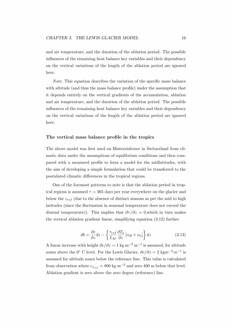
It is clear from the figures above, that as the size of the catchment is in-

creased, the impact of the glacier on runoff generation decreases. Infact, it


has little effect on the runoff from baseline 1961 - 1990 data and no effect

on runoff for projected climate change scenario using 2010 - 2039 IPSL data

(Figure 4.6).

The glacier presently occupies 0.31 km2, which accounts for 0.0155% of the

grid cell. As per the analyses above, this area is projected to decrease even

further and hence runoff generated from the meltwater of the glacier has

little effect on the catchment area. As per Figures 4.5 and 4.6 below, it can

be seen that as the size of the catchment is increased, the meltwater from

the glacier has no impact on the runoff generated in adjacent grid cells.

4.4 Climate variability and Runoff

From the above analyses, it was noted that the Lewis Glacier has little or no

effect on average annual runoff. The following figures show changes to runoff

in Kenya due to climate variability using the 5 models, CCMA CGCM31,

IPSL CM4, MPI ECHAM5, UKMO HADCM3, and NCAR CCM30 which

are based on IPCC SRES emssion scenario A1B for the years 2040 - 2069.

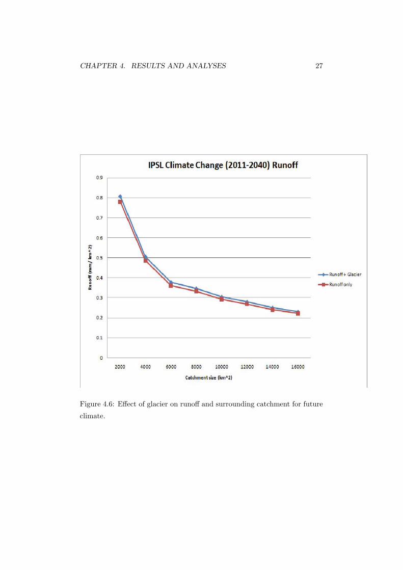
Figure 4.7 shows the average annual runoff between 1961 and 1990. It shows

higher runoff in the Rift Valley, Central Kenya, West Kenya and the Coast.

Average runoff in the North and North East of the country is less than half

of that in other parts. The model shows that there is highest runoff in the

Mount Kenya region.

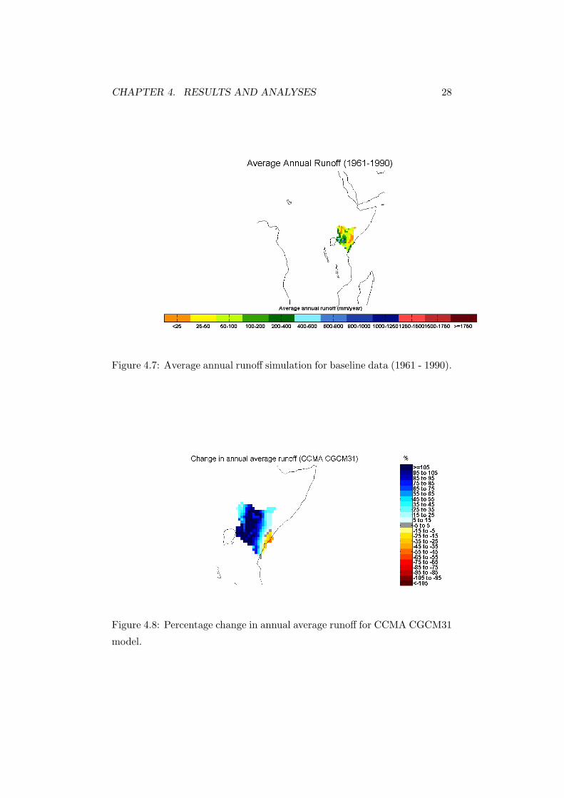
The CCMA CGCM31 model shows the highest increase in average runoff by

105% for most parts of Kenya and in particular the Rift Valley Region. In

contrast, the MPI ECHAM5 model simulates decrease in runoff in Western

Kenya by 15% and an increase in runoff in Eastern Kenya. All the models

show a decrease in runoff at the coast between 5 and 15% excpet NCAR

CCM30.

This bodes well for agricultural sector since tea and coffee farms are locared

in the highlands (Central Kenya) and horticultural farms are located in the

Rift Valley.


Figure 4.1: Observed and simulated mass balance profiles.


Figure 4.2: Specific mass balance profile simulations with different climate

change projections.


Figure 4.3: Projected area of Lewis Glacier over time.


Figure 4.4: Change in volume of glacier.


Figure 4.5: Effect of glacier on runoff and surrounding catchment for current

climate.


Figure 4.6: Effect of glacier on runoff and surrounding catchment for future

climate.


Figure 4.7: Average annual runoff simulation for baseline data (1961 - 1990).

Figure 4.8: Percentage change in annual average runoff for CCMA CGCM31

model.


Figure 4.9: Percentage change in annual average runoff for IPSL CM4 model.

Figure 4.10: Percentage change in annual average runoff for MPI ECHAM5

model.


Figure 4.11: Percentage change in annual average runoff for UKMO

HADCM3 model.

Figure 4.12: Percentage change in annual average runoff for NCAR CCM30

model.

Chapter 5

Discussion and Summary

5.1 Caveats

Caveats are associated with all components of the study - the glacier model,

the hydrological model, and in climate variability projections.

One of the key limitations of all the models is that estimation of current and

future mass balance profiles and runoff is based on simulated data and not

on observations. Therefore, any bias in the simulation model will be lead to

a bias in the projected changes (Arnell, 2004).

The glacier model does not simulate the specific mass balance to the cor-

rect amplitude. However, the simulations do model the longterm average

reasonably well as discussed earlier. This could be further investigated by

validating the model against other tropical glaciers. Another caveat is pre-

dicting the area covered by the glacier so as to determine the volume (in

water equivalent) stored by the glacier.

Although Euler’s method is not very accurate (doubling the number of

timesteps only halves the error) and converges slowly, it was deemed suffi-

cient since all the terms in equation 3.13 are linear. A Runge Kutta scheme

could be used to discretize the differential if the vertical accumulation gra-

dient is assumed to be non linear or if the scheme is applied to midlatitude

glaciers where the ablation term becomes non linear since δτ/ δz = 0.1.

It is assumed that all the water in the glacier will become meltwater and

31

CHAPTER 5. DISCUSSION AND SUMMARY 32

hence runoff. Interception by vegetaion, soil texture and evaporation have

been ignored. This would reduce the runoff generated due to meltwater even

further.

The hydrological model form and parameterisation is influenced and con-

strained by the availability of input data. Data sets used in the modelling

are gridded at different spatial resolution and some information is lost along

the way as it is interpolated down to the 0.5◦ × 0.5◦ resolution used in the

hydrological model.

Uncertainty in hydrological projections a rises from several sources:

•– Internal climate variability

– Emissions uncertainty

– Climate model uncertainty

– Simplification of processes, e.g. vegetation feedbacks, aerosols

– Downscaling and hydrological model uncertainty (Stott et al.,

2008

5.2 Conclusion

From the analysis carried out in Chapter 4, it can be concluded that the

Lewis Glacier is retreating at a relatively fast rate, the main factor driving

it being temperature. The area covered by the glacier will all but disappear

by 2039 if the current rate of decrease of 4.5% is kept up. Glaciers have

been known to retreat faster than has been predicted as per the IPCC 1997

and 2002 reports.

Furthermore, the glacier represents 0.0155% of the grid cell and thus has

little to no contribution to the streamflow of the region. However, using

climate change projections from 5 models based on A1B IPCC SRES emis-

sions, the Mac-PDM model predicts increased runoff in Kenya. More than

105% increase in some areas such as parts of the Rift Valley, Western and

Central Kenya are predicted while the North East and Eatern parts of Kenya

CHAPTER 5. DISCUSSION AND SUMMARY 33

may also see an increase in runoff which may relieve stress on the people

living in this semi-arid region at present.

5.3 Further Work

Due to time constraints and problems encountered during the study, the

following work could not be investigated but would add avlue to the study::

– Extend the simulations to other tropical glaciers and the effect

of climate variability on runoff from glacier melt;

– Develop a method to predict the change in the area covered by

the glacier based on physical concpets; and

– Incorporate the glacier model into the hydrological model to ac-

count for glacier meltwater contributions to streamflow at the

global level;

Other investigations could be based on the socio-economic impacts of melt-

ing of tropical and other glaciers, including changes in sea level.

Bibliography

[1] Arnell, N.W.(1999a) A simple water balance model for the sim-

ulation of streamflow over a large geographic domain, Journal of

Hydrology, 217, pp. 314–335.

[2] Arnell, N.W. (1999b) The effect of climate change on hydrological

regimes in Europe: a continental perspective, Global Environmen-

tal Change, 9, pp. 5–23.

[3] Arnell, N.W. (2003) Effect of IPCC SRES emission scenarios on

river runoff: a global perspective, Hydrology and Earth System

Science, 7, pp. 619–641.

[4] Arnell, N.W. (2004) Climate change and global water resources:

SRES emission and socio-economic scenarios, Global Environmen-

tal Change, 14, pp. 31–52.

[5] Bienn, D.I. and Evans, D.J.A (1998) Glaciers and Glaciation,

Arnold, London.

[6] ClimGen http://www.cru.uea.ac.uk/∼ timo/climgen/, cli-

matic Research Unit, (checked on 13.08.2009).

[7] Hastenrath, S. (1995) Glacier Recession on Mount

Kenya in the contect of global tropics, Bull. Inst. fr.

etudes andines,[Electronic], 24(3), pp. 633–638. Available:

http://www.ifeanet.org/publicaciones/boletines/24(3)/633.pdf,

(last checked on 15.08.2009).

34

BIBLIOGRAPHY 35

[8] Hock, R. (2005) Glacier melt: a review of processes and their

modelling, Progress in Physical Geography, 29, pp. 362–391.

[9] Innes, P. (2009) Tropical Weather Systems lecture notes

[10] IPPC (2001) Climate Change 2001:Work-

ing Group I: The Scientific Basis [electronic]

http://www.grida.no/publications/other/ipcctar/?src =

/CLIMATE/IPCCTAR/WG1/029.htm(checked21.08.2009)Karlen,W., Fastook, J.L.,Holmgren,K.,Malmstrom,M.,Matthews, J.A., Odada,E.,Risberg, J., Rosqvist,G., Sandgren, P., Shemesh,A., andWesterberg, L.(1999)GlacierF luctuationsonMountKenyasince∼6000 Cal. Years B.P: Implications for Holocene

Climatic Change in East Africa Ambio, pp. 409--418.

[11][12] Kaser, G. (2001) Glacier-Climate Interaction at Low

Latitudes, Journal of Glaciology, 47, pp 195--204.

[13] Kaser, G and Osmaston, H. (2002) Tropical Glaciers,

Cambridge University Press.

[14] Kuhn, M. (1980) Climate and Glaciers. Sea level,

ice and climatic change. (Proceedings of the Canberra

Symposium, Dec 1979), IAHS Publication Number, 131,

3--20. In Kaser, G and Osmaston, H. Tropical Glaciers,

Cambridge University Press, 2002.

[15] Ohmura, A. (2001) Physical Basis for the Temperature-Based

Melt Index Method, Journal of Applied Meteorology, 40, pp. 753–

761.

[16] Stott, P. (2008) Observed and projected changes in cli-

mate as they relate to water; Workshop on IPCC AR4

at Bonn Climate Change Talks - UNFCCC SBSTA 28th

Session - Bonn, Germany, 6 June 2008 [electronic] URL:

http://www.ipcc.ch/pdf/presentations/briefing-bonn-2008-06/observed-projected-changes%20.pdf

[17] Schaefli, B., Hingray,B., Niggli,M., and A. Musy (2005) A concep-

tual glacio-hydrological model for high mountainous catchments

Hydrology and Earth System Sciences, 9, pp. 95–105.

BIBLIOGRAPHY 36

[18] http://www.wri.org/publications/, World Resources Insti-

tute, (checked on 13.07.2009).

[19] Young, J. A. T and Hastenrath, S. (1991) Glaciers of the Mid-

dle East and Africa–Glaciers of Africa. Satellite Image Atlas of

Glaciers of the World US Geological Survey Professional Paper,

1386-G-3, G49–G70. In Karlen, W., Fastook, J.L., Holmgren,

K., Malmstrom, M., Matthews, J. A., Odada, E., Risberg, J.,

Rosqvist, G., Sandgren, P., Shemesh, A., and Westerberg, L.

(1999) Glacier Fluctuations on Mount Kenya since ∼ 6000 Cal.

Years B.P: Implications for Holocene Climatic Change in East

Africa Ambio, pp. 409–418.

impact and implications of climate variability and change

Documents