impact modified poly(ethylene terephthalate) …etd.lib.metu.edu.tr/upload/12605092/index.pdf · vi...

IMPACT MODIFIED POLY(ETHYLENE TEREPHTHALATE)-ORGANOCLAY

NANOCOMPOSITES

A THESIS SUBMITTED TO THE GRADUATE SCHOOL OF NATURAL AND APPLIED SCIENCES

OF MIDDLE EAST TECHNICAL UNIVERSITY

BY

ELİF ALYAMAÇ

IN PARTIAL FULFILLMENT OF THE REQUIREMENTS FOR

THE DEGREE OF MASTER OF SCIENCE IN

CHEMICAL ENGINEERING

JULY 2004

ii

Approval of the Graduate School of Natural and Applied Sciences

Prof. Dr. Canan Özgen

Director

I certify that this thesis satisfies all the requirements as a thesis for the degree of Master of Science.

Prof. Dr. Timur Doğu Head of Department

This is to certify that we have read this thesis and that in our opinion it is fully adequate, in scope and quality, as a thesis and for the degree of Master of Science.

Prof. Dr. Ülkü Yılmazer

Supervisor

Examining Committee Members

Prof. Dr. Nurcan Baç (METU, Che)

Prof. Dr. Ülkü Yılmazer (METU, Che)

Prof. Dr. Erdal Bayramlı (METU, Chem)

Assoc. Prof. Dr. Cevdet Kaynak (METU, Mete)

Assoc. Prof. Dr. Göknur Bayram (METU, Che)

iii

I hereby declare that all information in this document has been obtained and presented in accordance with academic rules and ethical conduct. I also declare that, as required by these rules and conduct, I have fully cited and referenced all material and results that are not original to this work. Name, Last name : Elif Alyamaç

Signature :

iv

ABSTRACT

IMPACT MODIFIED

POLY(ETHYLENE TEREPHTHALATE)-ORGANOCLAY

NANOCOMPOSITES

Alyamaç, Elif

M.S., Department of Chemical Engineering

Supervisor: Prof. Dr. Ülkü YILMAZER

July 2004, 113 pages

This study was conducted to investigate the effects of component

concentrations and addition order of the components, on the final properties of

ternary nanocomposites composed of poly(ethylene terephthalate), organoclay,

and an ethylene/methyl acrylate/glycidyl methacylate (E-MA-GMA) terpolymer

acting as an impact modifier for PET.

In this context, first, the optimum amount of the impact modifier was

determined by melt compounding binary PET-terpolymer blends in a corotating

twin-screw extruder. The amount of the impact modifier (5 wt. %) resulting in

the highest Young’s modulus and reasonable elongation at break was selected

owing to its balanced mechanical properties. Thereafter, by using 5 wt. %

terpolymer content, the effects of organically modified clay concentration and

addition order of the components on ternary nanocomposites were

systematically investigated.

Mechanical testing revealed that different addition orders of the materials

significantly affected mechanical properties. Among the investigated addition

orders, the best sequence of component addition (PI-C) was the one in which

poly(ethylene terephthalate) was first compounded with E-MA-GMA. Later, this

v

mixture was compounded with the organoclay in the subsequent run. Young's

modulus of not extruded pure PET increased by 67% in samples with 5 wt. % E-

MA-GMA plus 5 wt. % clay loading. The highest percent elongation at break was

obtained as 300%, for the addition order of PI-C, with 1 wt. % clay content,

which is nearly 50 fold higher than that obtained for pure PET.

In X-ray diffraction analysis, extensive layer separation associated with

delamination of the original clay structure occurred in PI-C and CI-P sequences

with both 1 and 3 wt. % clay contents. X-ray diffraction patterns showed that, at

these conditions exfoliated structures resulted as indicated by the disappearence

of any peaks due to the diffraction within the consecutive clay layers.

Keywords: poly(ethylene terephthalate), impact modification, organoclay,

nanocomposites, extrusion

vi

ÖZ

DARBE DAYANIMI İYİLEŞTİRİLMİŞ POLİETİLEN

TEREFTALAT- ORGANİK KİL NANOKOMPOZİTLERİ

Alyamaç, Elif

Yüksek Lisans, Kimya Mühendisliği

Tez Yöneticisi: Prof. Dr. Ülkü Yılmazer

Temmuz 2004, 113 sayfa

Bu çalışma, amorf polietilen tereftalat (PET), organik kil ve PET için darbe

iyileştirici olarak davranan etilen/metil akrilat/glisidil metakrilat (E-MA-GMA)

terpolimerinden oluşan üçlü nanokompozit sistemlerinin özelliklerine, bileşen

konsantrasyonlarının ve bileşen ekleme sırasının etkisini incelemek amacıyla

yürütülmüştür.

Bu çerçevede, ilk olarak, aynı yönde dönen çift vidalı ekstrüderde PET ve

darbe iyileştiricili sistemler eriyik halde karıştırılarak, en uygun darbe iyileştirici

miktarı belirlenmiştir. Young modülü yüksek, kopmadaki uzama değeri makul

olan darbe iyileştirici miktarı (ağırlıkça %5) dengeli mekanik özelliklerinden

dolayı seçilmiştir. Daha sonra, organik kil miktarı ve bileşenlerin ekleme

sırasının, ağırlıkça %5 darbe iyileştirici içeren, üçlü nanokompozit sistemleri

üzerindeki etkisi sistematik olarak incelenmiştir.

Mekanik testler, malzemelerin ekleme sırasının mekanik özellikleri büyük

ölçüde etkilediğini göstermiştir. PET’ in önce E-MA-GMA ile, daha sonra da

organik kille karıştırılması, en iyi ekleme sırası olmuştur. Ağırlıkça %5 kil ve %5

E-MA-GMA içeren numunelerde Young modülü, ekstrüzyon işlemine maruz

kalmamış PET’ e kıyasla %67 artış göstermiştir. En yüksek kopmada uzama

%300 olup bu değer saf PET’ inkinin yaklaşık 50 katıdır, ve ağırlıkça %1 kil

içeren PI-C sıralamasında elde edilmiştir.

vii

X-ışını kırınımı analizinde, kilin orijinal yapısının dağılmasına bağlı olarak

gözlemlenen tabaka açılması, PI-C ve CI-P sıralamalarında, ağırlıkça hem %1

hem de %3 kil içeriğinde oluşmuştur. X-ışını kırınımı grafiklerinde, çok iyi

dağılmış yapının oluştuğu, ardışık tabakalar arasında kırılmaya bağlı olarak

görülen tepe eğrilerinin kaybolmasından anlaşılmıştır.

Anahtar Kelimeler: poli(etilen tereftalat), darbe dayanımı iyileştirilmesi,

organik kil, nanokompozitler, ekstrüzyon

viii

To my family

ix

ACKNOWLEDGEMENTS

I would like to express my deepest gratitude to my supervisor Prof. Dr.

Ülkü Yılmazer, for his continuous support, encouragement and guidance

throughout this study.

I am very grateful to Assoc. Prof. Dr. Göknur Bayram from Department of

Chemical Engineering for giving me every opportunity to use the instruments in

her laboratory. I also would like to thank Prof. Dr. Erdal Bayramlı from

Department of Chemistry for letting me use the injection molding machine in his

laboratory and Prof. Dr Teoman Tinçer from Department of Chemistry for

providing me the impact test instrument in his laboratory.

Special thanks go to Cengiz Tan from Department of Metallurgical and

Materials Engineering for SEM Analysis and Mihrican Açıkgöz from Department of

Chemical Engineering for DSC Analysis.

İnciser Girgin and Bilgin Çiftçi from General Directorate of Mineral Research

and Exploration, for X-Ray Diffraction Analysis, are gratefully acknowledged. I

am also thankful to all my friends in Polymer Research Group for their

cooperation and friendship.

Last but not the least; I wish to express my sincere thanks to my family for

supporting, encouraging, and loving me all through my life.

x

TABLE OF CONTENTS

PLAGIARISM ........................................................................................... iii

ABSTRACT.............................................................................................. iv

ÖZ......................................................................................................... vi

DEDICATION..........................................................................................viii

ACKNOWLEDGEMENTS ............................................................................. ix

TABLE OF CONTENTS ................................................................................ x

LIST OF TABLES .....................................................................................xiii

LIST OF FIGURES ................................................................................... xv

NOMENCLATURE..................................................................................... xx CHAPTER

1. INTRODUCTION.................................................................................... 1

2. BACKGROUND ...................................................................................... 3

2.1 Composites .................................................................................... 3

2.1.1 Polymer Matrix Composites ...................................................... 3

2.2 Nanocomposites.............................................................................. 5

2.3 Polymer-Layered Silicate Nanocomposites........................................... 6

2.3.1 Layered Silicates .................................................................... 6

2.3.2 Structures of Polymer-Layered Silicate Nanocomposites .............. 8

2.4 Preparative Methods of Polymer-Layered Silicate Nanocomposites ........ 10

2.4.1 In-Situ Intercalative Polymerization Method.............................. 10

2.4.2 Solution Intercalation Method ................................................. 10

2.4.3 Melt Intercalation Method....................................................... 10

2.5 Polymer Processing........................................................................ 11

2.5.1 Extrusion............................................................................. 11

2.5.2 Injection Molding .................................................................. 12

xi

2.5.2.1 Melt Temperature ....................................................... 12

2.5.2.2 Injection Speed.......................................................... 12

2.5.2.3 Injection Pressure ...................................................... 12

2.6 Polymer Characterization................................................................ 13

2.6.1 Mechanical Properties ............................................................ 13

2.6.1.1 Tensile Test ............................................................... 13

2.6.1.2 Flexural Test.............................................................. 15

2.6.1.3 Impact Test ............................................................... 16

2.6.2 Thermal Analysis .................................................................. 17

2.6.2.1 Differential Scanning Calorimetry.................................. 17

2.6.3 Melt Viscosity/Rheology Measurements .................................... 19

2.6.3.1 Melt Flow Index.......................................................... 19

2.6.4 Morphological Analysis........................................................... 20

2.6.4.1 Scanning Electron Microscopy....................................... 20

2.6.5 X-Ray Diffraction .................................................................. 21

2.6.5.1 Principles of X-Ray Scattering and Diffraction ................. 21

2.7 Poly(ethylene terephthalate) ........................................................... 23

2.7.1 Chemistry............................................................................ 23

2.7.1.1 Melt-Phase Polycondensation....................................... 24

2.7.2 Morphology.......................................................................... 25

2.7.3 Degradation ......................................................................... 26

2.8 Literature Survey on Poly(ethylene terephthalate).............................. 27

2.8.1 Impact Modification of PET ..................................................... 27

2.8.2 PET/Clay Nanocomposites ...................................................... 28

3. EXPERIMENTAL................................................................................... 29

3.1 Materials ...................................................................................... 29

3.1.1 Polymer Matrix ..................................................................... 29

3.1.2 Layered Silicate .................................................................... 29

3.1.3 Impact Modifier .................................................................... 30

xii

3.2 Equipment and Processing .............................................................. 31

3.2.1 Melt Compounding ................................................................ 31

3.2.1.1 Addition Order of the Components ............................... 33

3.2.2 Injection Molding .................................................................. 38

3.3 Characterization............................................................................ 39

3.3.1 Mechanical Testing Procedure and Equipment ........................... 39

3.3.1.1 Tensile Test .............................................................. 40

3.3.1.2 Flexural Test............................................................. 41

3.3.1.3 Impact Test .............................................................. 42

3.3.2 Differential Scanning Calorimetry (DSC) Analysis....................... 43

3.3.3 Scanning Electron Microscopy (SEM) Analysis ........................... 43

3.3.4 X-Ray Diffraction Analysis ...................................................... 43

3.3.5 Melt Flow Index (MFI)............................................................ 44

4. RESULTS AND DISCUSSION ................................................................. 45

4.1 Morphological Analysis ................................................................... 45

4.1.1 X-Ray Diffraction Analysis ...................................................... 45

4.1.2 Scanning Electron Microscopy (SEM) Analysis ........................... 51

4.2 Flow Characteristics ....................................................................... 59

4.3 Mechanical Behavior ...................................................................... 61

4.3.1 Effect of Impact Modifier ........................................................ 61

4.3.2 Effects of Addition Order and Clay Concentration ....................... 65

4.4 Thermal Analysis........................................................................... 76

5. CONCLUSIONS ................................................................................... 79

REFERENCES ......................................................................................... 81

APPENDICES.......................................................................................... 87

A. Mechanical Testing Results................................................................... 87

B. DSC Thermograms.............................................................................. 95

C. X-ray Diffraction Patterns................................................................... 105

xiii

LIST OF TABLES

TABLE

2.1 Chemical structures of commonly used layered silicates ........................... 8

2.2 Comparison of extrusion to other plastics molding processes ................... 11

3.1 Typical Properties of APET .................................................................. 29

3.2 Physical Data of Cloisite 25A. .............................................................. 30

3.3 Specifications of E-MA-GMA ................................................................ 31

3.4 Drying temperature and time for the materials used in the study ............. 33

3.5 Formulation table. ............................................................................. 35

3.6 Molding parameters for all formulations ............................................... 38

3.7 Specifications of injection molded specimen .......................................... 41

4.1 X-ray diffraction results of materials containing clay............................... 46

4.2 MFI values of all formulations ............................................................. 60

4.3 Thermal properties of all formulations .................................................. 78

A.1 Arithmetic means and standard deviations of Young’s modulus values for

all formulations .............................................................................. 87

A.2 Arithmetic means and standard deviations of tensile strength values for


A.3 Arithmetic means and standard deviations of tensile stress at yield

values for all formulations ................................................................ 90

A.4 Arithmetic means and standard deviations of tensile strain at break

values for all formulations ................................................................ 91

A.5 Arithmetic means and standard deviations of flexural modulus values for


xiv

A.6 Arithmetic means and standard deviations of flexural strength values for


A.7 Arithmetic means and standard deviations of impact strength values for


xv

LIST OF FIGURES

FIGURE

2.1 Structure of 2:1 layered silicates ........................................................... 7

2.2 Schematic illustrations of a phase separated; an intercalated; and an

exfoliated polymer-layered silicate nanocomposites . ............................. 9

2.3 Tensile designations .......................................................................... 15

2.4 Schematic DSC curve ........................................................................ 18

2.5 Diffraction of x-rays by planes of atoms ............................................... 22

2.6 Chemical structure of PET................................................................... 23

2.7 Synthesis of PET with the transesterification reaction of DMT and EG ....... 24

3.1 Chemical structures of the quaternary ammonium and the anion; methyl

sulfate .......................................................................................... 30

3.2 Chemical structure of Lotader GMA AX8900 ......................................... 31

3.3 Processing temperatures of inlet, die, and mixing zones.......................... 32

3.4 Experimental setup for melt compounding ............................................ 32

3.5 Flowchart of (CI-P) two-step melt compounding procedure...................... 36

3.6 Flowchart of (PC-I) two-step melt compounding procedure...................... 36

3.7 Flowchart of (PI-C) two-step melt compounding procedure...................... 37

3.8 Flowchart of (All-S) two-step melt compounding procedure ..................... 37

3.9 Injection molding machine.................................................................. 39

3.10 Typical ASTM tensile test specimen .................................................... 40

3.11 Three-point loading diagram ............................................................. 41

3.12 Charpy-type impact instrument ......................................................... 42

4.1 X-ray diffraction patterns of nanocomposites containing 1 wt. % clay ....... 47


xvi


4.4 X-ray diffraction patterns of PET/clay nanocomposites with different clay

concentrations................................................................................ 50

4.5 SEM micrographs of double extruded, pure PET with magnifications: (a)

x250; (b) x3500 ............................................................................. 52

4.6 SEM micrographs of PET/E-MA-GMA blends with different E-MA-GMA

concentrations: (a) 5 wt. %, x250; (b) 5 wt. %, x3500; (c) 10 wt. %,

x250; (d) 10 wt. %, x3500 .............................................................. 52

4.7 SEM micrographs of PET/E-MA-GMA blends with different E-MA-GMA

concentrations: (a) 15 wt. %, x250; (b) 15 wt. %, x3500; (c) 20 wt.

%, x250; (d) 20 wt. %, x3500.......................................................... 53

4.8 SEM micrographs of PET/E-MA-GMA/C25A nanocomposites: (a) CI-P with

1 wt. % C25A, x250; (b) CI-P with 1 wt. % C25A, x3500; (c) CI-P with

3 wt. % C25A, x250; (d) CI-P with 3 wt. % C25A, x3500 ..................... 54

4.9 SEM micrographs of PET/E-MA-GMA/C25A nanocomposites: (a) PC-I with

1 wt. % C25A, x250; (b) PC-I with 1 wt. % C25A, x3500; (c) PC-I with

3 wt. % C25A, x250; (d) PC-I with 3 wt. % C25A, x3500; (e) PC-I with

5 wt. % C25A, x250; (f) PC-I with 5 wt. % C25A, x3500 ...................... 55

4.10 SEM micrographs of PET/E-MA-GMA/C25A nanocomposites: (a) PI-C

with 1 wt. % C25A, x250; (b) PI-C with 1 wt. % C25A, x3500; (c) PI-C

with 3 wt. % C25A, x250; (d) PI-C with 3 wt. % C25A, x3500; (e) PI-C

with 5 wt. % C25A, x250; (f) PI-C with 5 wt. % C25A, x3500 ............... 56

4.11 SEM micrographs of PET/E-MA-GMA/C25A nanocomposites: (a) All-S

with 1 wt. % C25A, x250; (b) All-S with 1 wt. % C25A, x3500; (c) All-

S with 3 wt. % C25A, x250; (d) All-S with 3 wt. % C25A, x3500; (e)

All-S with 5 wt. % C25A, x250; (f) All-S with 5 wt. % C25A, x3500 ....... 57

4.12 SEM micrographs of PET/C25A nanocomposites with different clay

concentrations: (a) 1 wt. % C25A, x250; (b) 1 wt. % C25A, x3500; (c)

xvii

3 wt. % C25A, x250; (d) 3 wt. % C25A, x3500; (e) 5 wt. % C25A,

x250; (f) 5 wt. % C25A, x3500......................................................... 58

4.13 The stress-strain curves for PET containing different amounts of impact

modifier ........................................................................................ 62

4.14 Young’s modulus values of PET/impact modifier blends as a function of

the impact modifier content ............................................................. 62

4.15 Tensile strain at break values of PET/impact modifier blends as a

function of the impact modifier content .............................................. 63

4.16 Tensile stress values of PET/impact modifier blends as a function of the

impact modifier content .................................................................. 63

4.17 Flexural strength and flexural modulus values of PET/impact modifier

blends as a function of the impact modifier content ............................. 64

4.18 The stress-strain curves of PET/clay (PC) nanocomposites containing

different amounts of clay. ............................................................... 66

4.19 The stress-strain curves of PET/impact modifier/clay nanocomposites

(PI-C) containing different amounts of clay. ....................................... 66


(PC-I) containing different amounts of clay. ....................................... 67


(CI-P) containing different amounts of clay. ....................................... 67


(All-S) containing different amounts of clay. ...................................... 68

4.23 Young’s modulus values of all formulations as a function of clay

concentration. ............................................................................... 68

4.24 Tensile strength as a function of clay content ...................................... 70

4.25 Tensile strain at break (%) as a function of clay content ....................... 70

4.26 Tensile stress at yield as a function of clay content............................... 72

4.27 Impact strength as a function of clay content ...................................... 72

xviii

4.28 Flexural modulus as a function of clay content ..................................... 74

4.29 Flexural strength as a function of clay content ..................................... 74

B.1 DSC thermogram of not extruded, pure PET.......................................... 95

B.2 DSC thermogram of impact modifier (E-MA-GMA) .................................. 96

B.3 DSC thermogram of double extruded PET ............................................. 96

B.4 DSC thermogram of PC with 1 wt. % clay content.................................. 97



B.7 DSC thermogram of PI with 5 wt. % E-MA-GMA content ......................... 98

B.8 DSC thermogram of PI with 10 wt. % E-MA-GMA content ....................... 99

B.9 DSC thermogram of PI with 15 wt. % E-MA-GMA content ....................... 99

B.10 DSC thermogram of PI with 20 wt. % E-MA-GMA content.................... 100

B.11 DSC thermogram of CI-P with 1 wt. % clay content............................ 100

B.12 DSC thermogram of CI-P with 3 wt. % clay content............................ 101

B.13 DSC thermogram of PC-I with 1 wt. % clay content............................ 101



B.16 DSC thermogram of PI-C with 1 wt. % clay content............................ 103



B.19 DSC thermogram of All-S with 1 wt. % clay content ........................... 104



C.1 X-ray diffraction patterns of PC with 1 wt. % clay content .................... 106



C.4 X-ray diffraction patterns of CI-P with 1 wt. % clay content ................. 108

C.5 X-ray diffraction patterns of CI-P with 3 wt. % clay content ................. 108

xix

C.6 X-ray diffraction patterns of PC-I with 1 wt. % clay content ................. 109



C.9 X-ray diffraction patterns of PI-C with 1 wt. % clay content ................. 110

C.10 X-ray diffraction patterns of PI-C with 3 wt. % clay content ................ 111

C.11 X-ray diffraction patterns of PI-C with 5 wt. % clay content ................ 111

C.12 X-ray diffraction patterns of All-S with 1 wt. % clay content ............... 112



xx

NOMENCLATURE

A0 Original, undeformed cross-sectional area, mm2

b Width of beam tested, mm

c velocity of light, m/s

d Depth of beam tested, mm

d Plane spacing, Å

D Distance, mm

E Modulus of Elasticity, MPa

EB Modulus of elasticity in bending, MPa

F Tensile Load, N

h Plank’s constant, J.sec

L Support span, mm

L0 Initial gauge length, mm

∆L Change in sample length, mm

m Slope of the tangent to the initial straight-line portion of the load-

deflection curve, N/mm

M Monovalent cation

n Order of diffraction

P Load at a given point on the load-deflection curve, N

R Maximum strain in the outer fibers, mm/mm

S Stress in the outer fibers at midspan, MPa

T Thickness, mm

Tc Crystallization temperature, °C

Tg Glass transition temperature, °C

Tm Melting temperature, °C

W Width, mm

x Degree of isomorphous substitution

xxi

Greek Letters

Є Tensile strain, mm/mm

λ Wavelength, nm

ν Frequency

σ Tensile stress(nominal), MPa

σm Tensile strength, MPa

θ Scattering angle, °

Abbreviations

APET Amorphous Poly(Ethylene Terephthalate)

ASTM American Society for Testing and Materials

BHET Bis (β-Hydroxyethyl) Terephthalate

CEC Cation Exchange Capacity

DMT Dimethyl Terephthalate

DSC Differential Scanning Calorimetry

EG Ethylene Glycol

E-GMA Ethylene-Glycidyl Methacrylate

E-MA-GMA Ethylene-Methyl Acrylate-Glycidyl Methacrylate

EPR Ethylene-co-Propylene Rubber

GMA Glycidyl Methacrylate

HT Hydrogenated Tallow

IV Intrinsic Viscosity

MFI Melt Flow Index

MMT Montmorillonite

PET Poly(Ethylene Terephthalate)

PLS Polymer Layered Silicate

PTA Purified Terephthalic Acid

SAXS Small Angle X-ray Scattering

SEM Scanning Electron Microscopy

TEM Transmission Electron Microscopy

TPA Terephthalic Acid

WAXS Wide Angle X-ray Scattering

XRD X-Ray Diffraction

1

CHAPTER 1

INTRODUCTION

Composite materials are a new class of materials that combine two or more

distinctly dissimilar components into a suitable form. While each component

retains its identity, the new composite material displays macroscopic properties

superior to its parent constituents, particularly in terms of mechanical properties

and economic value (Broutman and Krock, 1967).

In recent years, it is found that when fillers are dispersed in polymers on

the nanometer scale, composites obtained show improved properties compared

to conventional polymer composites. Among these properties improved by the

presence of nanofillers are mechanical, thermal, physical and barrier properties.

This new class of composites is called polymer matrix nanocomposites

(Giannelis, 1996).

Today, studies are being conducted globally, using almost all types of

polymer matrices. Consequently, current reports on poly(ethylene terephthalate)

based nanocomposites (Pinnavaia and Beall, 2000) and impact modification of

poly(ethylene terephthalate) (Chapleau and Huneault, 2003) exist in the

literature. However, there are no studies on nanocomposites formed from

organically modified clay as the reinforcing agent and impact modified

poly(ethylene terephthalate) as the matrix.

Poly(ethylene terephthalate) is a thermoplastic polyester having poor

impact resistance and high notch sensitivity. Additionally, in PET/clay

nanocomposites, addition of clay sometimes imparts drawbacks to the resulting

material such as brittleness. For this reason, impact modification of PET can be

achieved by dispersing elastomeric polymers in the polymer matrix.

2

In this study, the effects of component concentrations and addition order

of the components, on the final properties of ternary nanocomposites composed

of amorphous poly(ethylene terephthalate) matrix, organically modified clay, and

an ethylene/methyl acrylate/glycidyl methacylate (E-MA-GMA) terpolymer were

systematically investigated.

In this context, first, the amount of the terpolymer acting as an impact

modifier for PET was optimized by melt compounding binary PET-terpolymer

blends. The amount of the impact modifier resulting in the highest elastic

modulus and reasonable elongation at break was selected owing to its balanced

mechanical properties. Thereafter, by using the optimum impact modifier

concentration, the effects of organically modified clay concentration and addition

order of the components were systematically investigated by preparing ternary

nanocomposites formed from organically modified clay as the nanofiller and

impact modified poly(ethylene terephthalate) as the matrix.

All formulations were prepared by melt compounding of the components

with a two-step mixing procedure in a corotating twin-screw extruder. Prior to

characterization, standard test specimens were injection molded. Mechanical

tests conducted on each composition included the investigation of tensile

strength, Young’s modulus, tensile stress at yield, percent elongation at break,

flexural modulus, flexural strength and impact strength. The morphology was

analyzed by X-Ray Diffraction and Scanning Electron Microscopy. Flow

characteristics, melting and crystallization behavior of the compositions were

also studied by Melt Flow Index Measurements and Differential Scanning

Calorimetry Analysis, respectively.

At the end of the study, the processing parameters of the nanocomposites

were optimized using the properties synergistically derived from the three

components.

3

CHAPTER 2

BACKGROUND

2.1 Composites

A composite is a multiphase material that exhibits a significant proportion

of the properties of both constituent phases such that a better combination of

properties is realized. Many composite materials are composed of just two

phases; one is termed the matrix, which is continuous and surrounds the other

phase, often called the dispersed phase. The properties of composites are a

function of the properties of the constituent phases, their relative amounts, and

the geometry of the dispersed phase. "Dispersed phase geometry" in this

context means the shape of the particles and the particle size, distribution, and

orientation (Callister, 1997).

2.1.1 Polymer Matrix Composites

Polymers, metals, and ceramics are all used as matrix materials in

composites, depending on the particular requirements. Polymers are

unquestionably the most widely used matrix materials in modern composites

(Gibson, 1994). Polymers have advantages over other types of materials, such

as metals and ceramics, because their low processing costs, low weight and

properties such as transparency and toughness form unique combinations. Many

polymers have useful characteristics, such as tensile strength, modulus,

elongation and impact strength and make them more cost effective than metals

and ceramics (Sawyer and Grubb, 1987).

A polymer is defined as a long-chain molecule built up by the repetition of

small, simple chemical units. In some cases the repetition is linear, much as a

chain is built up from its links. In other cases the chains are branched or

4

interconnected to form three-dimensional networks. The repeat unit of the

polymer is usually equivalent or nearly equivalent to the monomer, or starting

material from which the polymer is formed (Billmeyer, 1984).

Polymers are divided into two broad categories: thermoplastics and

thermosets. In a thermoplastic polymer, individual molecules are linear in

structure with no chemical linking between them. They are held in place by weak

secondary bonds such as van der Waals forces and hydrogen forces. With the

application of heat and pressure, these intermolecular bonds in a solid

thermoplastic polymer can be temporarily broken and the molecules can be

moved relative to each other to flow into new positions. Upon cooling, the

molecules freeze in their new positions, restoring the secondary bonds between

them and resulting in a new solid shape. Thus, a thermoplastic polymer can be

heat-softened, melted and reshaped as many times as desired.

In a thermoset polymer, on the other hand, the molecules are chemically

joined together by cross-links, forming a rigid, three-dimensional network

structure. Once these cross-links are formed during the polymerization reaction,

the thermoset polymer can not be melted and reshaped by the application of

heat and pressure.

The primary consideration in the selection of a matrix is its basic

mechanical properties including tensile modulus, tensile strength, and fracture

toughness. The most important advantage of thermoplastic polymers over

thermoset polymers is their high impact strength and fracture resistance, which

in turn impart excellent damage tolerance characteristics to the composite

material (Schwartz, 1997). In general, thermoplastic polymers have higher

strains to failure than thermoset polymers, which may provide a better

resistance to matrix microcracking in the composite laminate.

5

2.2 Nanocomposites

For some time, particles have been added to polymers in order to

improve the stiffness and the toughness of the materials, to enhance their

barrier properties, to enhance their resistance to fire and ignition or just simply

to reduce cost. In recent years, it was found that when the fillers are dispersed

in polymers on the nanometer scale, the materials possessed unique properties

typically not shared by their more conventional microcomposite counterparts.

This new class of materials is called nanocomposites (Giannelis, 1996).

Nanocomposites already look attractive for molded car parts such as body

panels and under-hood components, as well as electrical/electronic parts, power-

tool housings, lawnmowers, aircraft interiors, and applier components. On the

packaging side, nanocomposites can slow down transmission of gases and

moisture vapor through plastics by creating a "tortuous path" for gas molecules

to thread their way among the obstructing platelets (Sherman L.M., 1999).

Polymer nanocomposites are particle-filled polymers in which at least one

dimension of the dispersed particles is in the nanometer range. One can

distinguish three types of polymer nanocomposites, depending on how many

dimensions of the dispersed particles are in the nanometer range. When all three

dimensions are on the nanometer scale, they are called isodimensional

nanoparticles or zero-dimension reinforcing particles (Mark, 1996; Herron and

Thorn, 1998); when two dimensions are in the nanometer scale and the third is

larger, they are called nanotubes/nanofibers or one-dimension reinforcing

particles (Favier et al., 1997; Chazeau et al., 1999). This type of nanocomposite

is extensively studied because reinforcing nanofillers yield materials with

exceptional properties.

The third type of nanocomposites has fillers with only one dimension in

the nanometer range that reinforce the material in two dimensions. For this type

of nanocomposite, the fillers are present in a form of sheets with a thickness of a

few nanometers and hundred to thousands nanometers of length and width

(Alexandre and Dubois, 2000). In our study, we have focused on the third type

of nanocomposites which is to be explained in the following section.

6

2.3 Polymer-Layered Silicate Nanocomposites

After layered silicates are dispersed on a nanometer scale into the

polymer matrix, nanocomposites exhibit significantly improved mechanical,

thermal, optical and physico-chemical properties when compared with pure

polymer or conventional composites. Improvements may include, for instance,

increased modulus, strength, heat resistance, decreased gas permeability and

flammability.

The unprecedented mechanical properties of polymer layered silicate

nanocomposites (PLS) were first demonstrated by researchers at Toyota using

nylon nanocomposites (Kojima et al., 1993). They showed that a doubling of the

tensile modulus and strength is achieved for nylon-layered silicate

nanocomposites containing as little as 2 vol. % inorganic material.

PLS nanocomposites have several advantages (Giannelis, 1999) e.g. (a)

they are lighter in weight compared to conventionally filled polymers because

high degrees of stiffness and strength are realized with far less high density

inorganic material; (b) they exhibit outstanding diffusional barrier properties

without requiring a multipolymer layered design, allowing for recycling; and (c)

their mechanical properties are potentially superior to unidirectional fiber

reinforced polymers, because reinforcement from the inorganic layers will occur

in two rather than in one dimension. Uses for this new class of composites can

be found in aerospace, automotive, electronics and biotechnology applications,

to list only a few (Schmidt et al., 2002).

2.3.1 Layered Silicates

The layered silicates used in polymer-layered silicate nanocomposites, like

the better known members of the group, talc and mica, belong to the structural

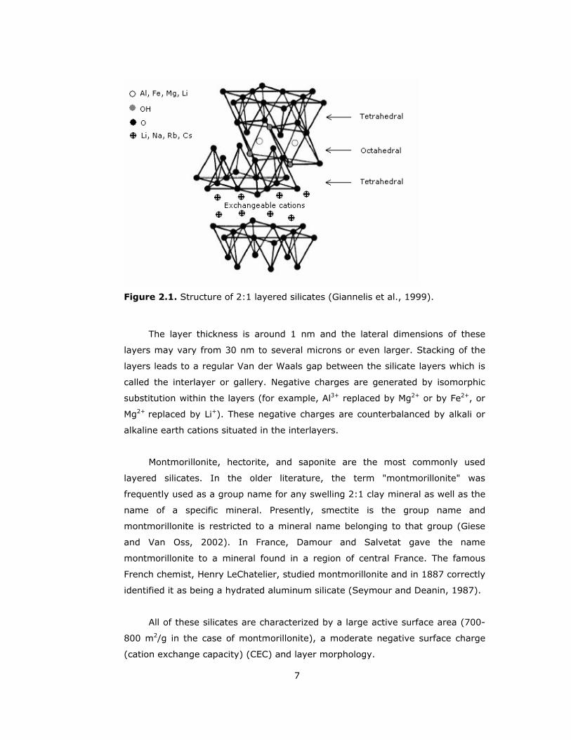
family of 2:1 phyllosilicates. Their crystal structure consists of multi-layers. Each

layer is made up of two silica tetrahedral sheets and an edge-shared octahedral

sheet of either aluminum or magnesium hydroxide. Their structure is shown in

Figure 2.1 and their chemical formulas are given in Table 2.1.

7

Figure 2.1. Structure of 2:1 layered silicates (Giannelis et al., 1999).

The layer thickness is around 1 nm and the lateral dimensions of these

layers may vary from 30 nm to several microns or even larger. Stacking of the

layers leads to a regular Van der Waals gap between the silicate layers which is

called the interlayer or gallery. Negative charges are generated by isomorphic

substitution within the layers (for example, Al3+ replaced by Mg2+ or by Fe2+, or

Mg2+ replaced by Li+). These negative charges are counterbalanced by alkali or

alkaline earth cations situated in the interlayers.

Montmorillonite, hectorite, and saponite are the most commonly used

layered silicates. In the older literature, the term "montmorillonite" was

frequently used as a group name for any swelling 2:1 clay mineral as well as the

name of a specific mineral. Presently, smectite is the group name and

montmorillonite is restricted to a mineral name belonging to that group (Giese

and Van Oss, 2002). In France, Damour and Salvetat gave the name

montmorillonite to a mineral found in a region of central France. The famous

French chemist, Henry LeChatelier, studied montmorillonite and in 1887 correctly

identified it as being a hydrated aluminum silicate (Seymour and Deanin, 1987).

All of these silicates are characterized by a large active surface area (700-

800 m2/g in the case of montmorillonite), a moderate negative surface charge

(cation exchange capacity) (CEC) and layer morphology.

8

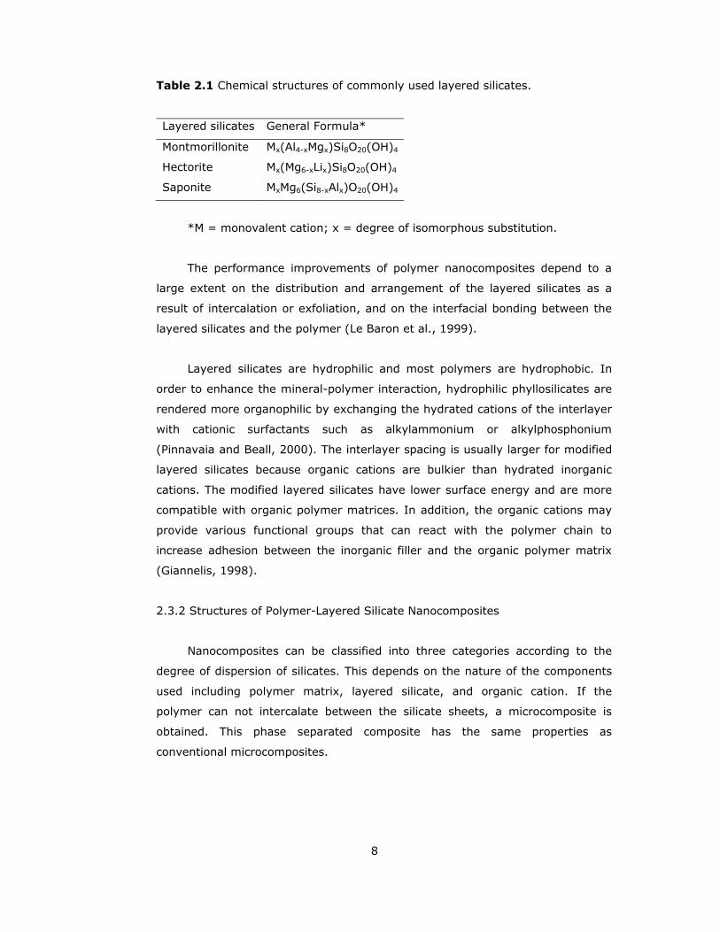
Table 2.1 Chemical structures of commonly used layered silicates.

Layered silicates General Formula*

Montmorillonite Mx(Al4-xMgx)Si8O20(OH)4

Hectorite Mx(Mg6-xLix)Si8O20(OH)4

Saponite MxMg6(Si8-xAlx)O20(OH)4

*M = monovalent cation; x = degree of isomorphous substitution.

The performance improvements of polymer nanocomposites depend to a

large extent on the distribution and arrangement of the layered silicates as a

result of intercalation or exfoliation, and on the interfacial bonding between the

layered silicates and the polymer (Le Baron et al., 1999).

Layered silicates are hydrophilic and most polymers are hydrophobic. In

order to enhance the mineral-polymer interaction, hydrophilic phyllosilicates are

rendered more organophilic by exchanging the hydrated cations of the interlayer

with cationic surfactants such as alkylammonium or alkylphosphonium

(Pinnavaia and Beall, 2000). The interlayer spacing is usually larger for modified

layered silicates because organic cations are bulkier than hydrated inorganic

cations. The modified layered silicates have lower surface energy and are more

compatible with organic polymer matrices. In addition, the organic cations may

provide various functional groups that can react with the polymer chain to

increase adhesion between the inorganic filler and the organic polymer matrix

(Giannelis, 1998).

2.3.2 Structures of Polymer-Layered Silicate Nanocomposites

Nanocomposites can be classified into three categories according to the

degree of dispersion of silicates. This depends on the nature of the components

used including polymer matrix, layered silicate, and organic cation. If the

polymer can not intercalate between the silicate sheets, a microcomposite is

obtained. This phase separated composite has the same properties as

conventional microcomposites.

9

Figure 2.2 Schematic illustrations of a phase separated; an intercalated; and an exfoliated polymer-layered silicate nanocomposites.

Beyond this traditional class of polymer-filler composites, two types of

nanocomposites can be obtained: Intercalated structures are formed when a

single (or sometimes more) extended polymer chain is intercalated between the

silicate layers. The result is a well ordered multilayer structure of alternating

polymeric and inorganic layers (Beyer, 2002).

In an exfoliated or delaminated nanocomposite, the silicates are completely

and uniformly dispersed in the continuous polymer matrix. Usually, the clay

content of an exfoliated nanocomposite is much lower than that of an

intercalated nanocomposite (Yoon et al., 2001).

The delamination configuration is of particular interest because it

maximizes the polymer-clay interactions, making the entire surface of the layers

available for the polymer. This should lead to the most significant changes in

mechanical and physical properties. Possible polymer-layered silicate structures

are given in Figure 2.2.

Layered silicate Polymer

Phase separated Intercalated Exfoliated (microcomposite) (nanocomposite) (nanocomposite)

10

2.4 Preparative Methods of Polymer-Layered Silicate Nanocomposites

The preparative methods are divided into three main groups according to

the starting materials and processing techniques.

2.4.1 In-situ Intercalative Polymerization Method

In this method, the layered silicate is swollen within the liquid monomer

or a monomer solution so the polymer formation can occur between the

intercalated sheets. Polymerization can be initiated either by heat or radiation,

by the diffusion of a suitable initiator, or by an organic initiator or catalyst fixed

through cation exchange inside the interlayer before the swelling step. It is the

first method used to synthesize polymer-layered silicate nanocomposites based

on polyamide 6 (Fukushima et al., 1988).

2.4.2 Solution Intercalation Method

This is based on a solvent system in which the polymer is soluble and the

silicate layers are swellable. The layered silicate is first swollen in a solvent, such

as water, chloroform, or toluene. When the polymer and layered silicate

solutions are mixed, the polymer chains intercalate and displace the solvent

within the interlayer of the silicate (Sinha Ray et al., 2003). Upon solvent

removal, the intercalated structure remains resulting in PLS nanocomposite.

2.4.3 Melt Intercalation Method

This method was first reported by Vaia et al. in 1993. The process

involves annealing a mixture of polymer and layered silicates above melting

point of the polymer. During the anneal, the polymer chains diffuse from the

bulk polymer melt into the van der Waals galleries between the silicate layers

(Vaia et al., 1995). This method is quite general and is broadly applicable to a

range of commodity polymers from essentially non-polar polystyrene, to weakly

polar poly(ethylene terephthalate), to strongly polar nylon.

It has great advantages over either in-situ intercalative polymerization or

solution intercalation. First, this method is environmentally benign due to the

absence of organic solvents. Second, it is compatible with current industrial

process, such as extrusion and injection molding. The melt intercalation method

11

allows the use of polymers which were previously not suitable for in situ

polymerization or solution intercalation. Besides, it is a quite effective technology

for the case of polyolefin-based nanocomposites (Hasegawa et al., 2000).

2.5 Polymer Processing

2.5.1 Extrusion

In principle, the extrusion process comprises the forcing of a plastic or

molten material through a shaped die by means of pressure (Morton-Jones D.H.,

1989). In addition to the shaping of parts by the extrusion process, extrusion is

the most efficient and widely used process for melting plastic resin as part of the

process of adding or mixing fillers, colorants, and other additives into the molten

plastic. Extrusion can be used to shape the part directly after this mixing or an

extruder can be used as the melting device that is coupled with other shaping

processes (Strong, 1996). Examples of the use of extruders as integral parts of

other plastic forming operations would include injection molding, blow molding,

and foam making. The advantages and disadvantages of extrusion are

summarized in Table 2.2.

Table 2.2 Comparison of extrusion to other plastics molding processes.

Advantages Disadvantages

Continuous Limited complexity of parts

High production volumes Uniform cross-sectional shape only

Low cost per pound

Efficient melting

Many types of raw materials

Good mixing (compounding)

Twin-screw extruders are a widely used type of extruders. They exist in

corotating and counterrotating versions; the screws could be non-intermeshing,

partially intermeshing or closely intermeshing. With corotating twin-screw

extruders, the melt contained in one screw channel is transferred to the other

channel with each rotation. The transport mechanism (drag forces) is

comparable to that of a single-screw extruder. The melt however is exposed to a

greater shear stress due to the increased path length through the extruder.

12

Such extruders are almost exclusively employed for compounding (Ullmann's

Encyclopedia of Industrial Chemistry, 1992).

2.5.2 Injection Molding

Many well known thermoplastic processes rely on an extrusion system to

provide the heat-softened material for manipulation into a final finished article.

Injection molding is an obvious and possibly the oldest example of this where a

thermoplastic material is forced by a ram through a heating chamber and then to

a nozzle or die and finally into a closed mold where the material takes up the

required form (Fisher, 1976).

There are several configurations of injection units in use today. The

simplest, first generation plunger and torpedo machines are still being made, but

the most widely used type is the reciprocating single-screw injection unit

(Schwartz, 1997). The most important process parameters controlled by the

injection unit are the following.

2.5.2.1 Melt Temperature

The temperature of the melt when it penetrates into the mold is

controlled by the temperature control system of the injection unit but may also

be affected by the injection speed and by the level of back pressure.

2.5.2.2 Injection Speed

This is the speed at which the screw advances during the mold filling

step. Modern machines are equipped with variable injection speed control- a

profile of speeds rather than a single constant value is used to fill the mold.

Typical mold filling starts at a low speed to prevent jetting; speed is increased

during the middle part of filling and reduced again toward the end to allow

smooth and accurate transition to pressure control, which takes over when the

mold is full.

2.5.2.3 Injection Pressure

The pressure exerted by the screw on the melt is not constant during the

mold filling stage. Injection pressure builds up as the mold is filled and as the

13

resistance to flow increases. It is only when the mold is full that a transfer from

speed control to pressure control takes place. Injection pressure is the principle

variable during the holding stage.

2.6 Polymer Characterization

Once a new material is developed, its properties should be evaluated and

usually compared with the properties of already known materials to verify the

proposed reaction. Analysis of properties of newly developed material is also

important in determining the applications for which the material can be used.

There are various analytical and evaluative methods currently available. Many of

them are equipped with high technology device with computer programs.

Although there is no single test that can provide all the answers needed, one can

obtain a good picture of the type of material by combining the results of various

tests. The methods and their standard procedures used in this study will be

discussed in the following sections.

2.6.1 Mechanical Properties

There are a variety of methods which are useful in predicting mechanical

properties of polymers. However, it is essential that there should be some

consistency in the manner in which tests are conducted, and in the interpretation

of their results. This consistency is accomplished by using standardized testing

techniques. Establishment and publication of these standards are often

coordinated by professional societies. In the United States the most active

organization is the American Society for Testing and Materials (ASTM). Its annual

book of ASTM standards comprises numerous volumes, which are issued and

updated yearly; a large number of these standards relate to mechanical testing

techniques. Three of the more commonly employed testing techniques based on

ASTM standards are tensile, flexural and impact tests.

2.6.1.1 Tensile Test

Standard test method for tensile properties (ASTM D638M-91a) employs

specimens of a specified shape, typically a dogbone, as depicted in Figure 3.10.

During the test, a specimen is deformed, usually to fracture, with a gradually

increasing tensile load that is applied uniaxially along the long axis of a

14

specimen. The length of the center section is called the initial gauge length L0.

The force F is measured at the fixed end as a function of elongation.

σ = F / A0 (2.1)

Є = ∆L / L0 (2.2)

where A0 is the original, undeformed cross-sectional area of the gauge region

and ∆L is the change in sample length as a result of the applied force.

Tensile stress (nominal), σ is the tensile load per unit area of minimum

original cross-section, with the gauge boundaries, carried by the test specimen

at any given moment. It is expressed in force per unit area, usually in

megapascals, (Equation 2.1).

Tensile strength, σm is the maximum tensile stress sustained by the

specimen during a tension test. When the maximum stress occurs at the yield

point, it is designated tensile strength at yield. When the maximum stress occurs

at break, it is designated tensile strength at break.

Tensile strain, Є is the ratio of the elongation to the gauge length of the

test specimen, that is, the change in length per unit of original length. It is

expressed as a dimensionless ratio, as shown in Equation 2.2.

It is seen in Equation 2.3 that modulus of elasticity, E is the ratio of stress

(nominal) to corresponding strain below the proportional limit of a material. It is

expressed in force per unit area, usually in megapascals. It is also known as

elastic modulus or Young's modulus.

E = σ / Є (2.3)

15

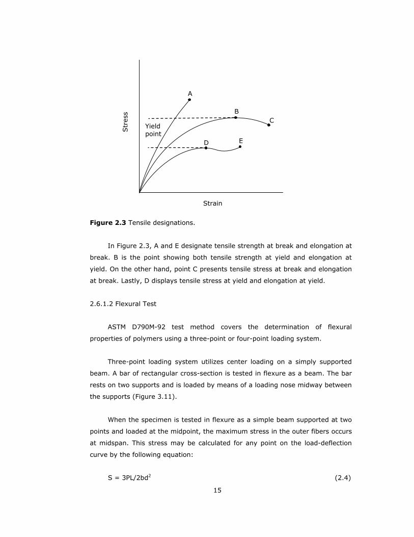
Figure 2.3 Tensile designations.

In Figure 2.3, A and E designate tensile strength at break and elongation at

break. B is the point showing both tensile strength at yield and elongation at

yield. On the other hand, point C presents tensile stress at break and elongation

at break. Lastly, D displays tensile stress at yield and elongation at yield.

2.6.1.2 Flexural Test

ASTM D790M-92 test method covers the determination of flexural

properties of polymers using a three-point or four-point loading system.

Three-point loading system utilizes center loading on a simply supported

beam. A bar of rectangular cross-section is tested in flexure as a beam. The bar

rests on two supports and is loaded by means of a loading nose midway between

the supports (Figure 3.11).

When the specimen is tested in flexure as a simple beam supported at two

points and loaded at the midpoint, the maximum stress in the outer fibers occurs

at midspan. This stress may be calculated for any point on the load-deflection

curve by the following equation:

S = 3PL/2bd2 (2.4)

Yield point

E D

C B

A

Str

ess

Strain

16

where S is stress in the outer fibers at midspan (MPa), P is load at a given point

on the load-deflection curve (N), L is support span (mm), b is width of beam

tested (mm), and d is depth of beam tested (mm).

The maximum strain in the outer fibers occurs at midspan as well, and may

be calculated as follows:

r = 6Dd/L2 (2.5)

where r is maximum strain in the outer fibers (mm/mm), D is maximum

deflection of the center of the beam (mm), d is depth of beam tested (mm), and

L is support span (mm).

The tangent modulus of elasticity, often called flexural modulus, is the ratio

within the elastic limit of stress to corresponding strain and shall be expressed in

megapascals. It is calculated by drawing a tangent to the steepest initial

straight-line portion of the load-deflection curve and using Equation 2.6.

EB = L3m/4bd3 (2.6)

where EB is modulus of elasticity in bending (MPa), L is support span (mm), b is

width of beam tested (mm), d is depth of beam tested (mm), and m is slope of

the tangent to the initial straight-line portion of the load-deflection curve

(N/mm).

2.6.1.3 Impact Test

Another popular method of testing (ASTM D256-92) the mechanical

performance of polymers involves impact loading. Here, a specimen, often with a

sharp notch cut in it, is struck a sudden blow, causing failure. Impact tests

measure the energy required for failure when a standard specimen receives a

rapid stress loading.

The impact strength of a polymer can be measured employing a number of

techniques including Izod and Charpy tests. For both Izod and Charpy tests, a

17

weight is released, causing the specimens to be struck. The energy to break

values are determined from the loss in the kinetic energy of the weight.

Impact tests are not limited to the basic Charpy and Izod methods. Special

purpose tests, sometimes very highly instrumented, are used to characterize

polymer blends and composites (Sperling, 1997).

2.6.2 Thermal Analysis

Thermal analysis represents a wide range of analytical techniques designed

to assess the response of materials to thermal stimuli, typically temperature

change. Various techniques evaluate changes in enthalpy, specific heat, thermal

conductivity and diffusivity, linear and volumetric expansion, mechanical and

viscoelastic properties with temperature.

2.6.2.1 Differential Scanning Calorimetry

The differential scanning calorimeter (DSC) is the instrument that has

dominated the field of thermal analysis in the past decade. The term DSC was

coined in 1963 at Perkin-Elmer to describe a new thermal analyzer they had

developed (Watson et al., 1964). It measures heat flows and temperatures

associated with exothermic and endothermic transitions. The ease with which

important properties such as transitions, heat capacity, reaction, and

crystallization kinetics are characterized has made the DSC widely used in the

plastics laboratory (Lobo and Bonilla, 2003).

In DSC analysis, two identical small sample pans are instrumented to

operate at the same temperature and can be programmed up or down in

temperature at the same rate. A sample is placed in one, and the other is left

empty. Instrumentation is provided to measure the electrical power necessary to

keep the two sample pans at the same temperature. If a temperature is

encountered at which the sample undergoes a change of phase or state, more or

less power will be needed to keep the sample pan at the same temperature as

the reference pan (depending on whether the reaction is exothermic or

endothermic).

Since power is the value being recorded, the area under the peak is the

electrical equivalent of the heat of the reaction. To measure heat capacity in this

18

calorimeter, the sample pan and reference pan are first brought to some

temperature and then heated at some constant rate. Since the reference pan is

empty, it will require a smaller amount of electrical power to achieve this rate

(Encyclopedia of Polymer Science and Technology, 1970).

Some advantages of the differential scanning calorimeter are that relatively

short times are required to make a determination and that small sample size is

sufficient. The disadvantage is that it is a comparative rather than an absolute

method.

Figure 2.4 Schematic DSC curve.

DSC is routinely used for investigation, selection, comparison, and end-use

performance of materials. It is used in academic, industrial, and government

research facilities, as well as quality control and production operations. Material

properties measured include glass transitions, melting point, freezing point,

boiling point, decomposition point, crystallization, phase changes, melting,

crystallization, product stability, cure and cure kinetics, and oxidative stability.

Crystallization

Melting Tg Tm

Endoth

erm

ic H

eat

Flow

Rat

e Exo

ther

mic

Temperature

19

At Tg, the heat capacity of the sample suddenly increases, requiring more

power (relative to the reference) to maintain the temperatures the same. This

differential heat flow to the sample (endothermic) causes a drop in the DSC

curve (Figure 2.4). At Tm, the sample crystals want to melt at constant

temperature, so a sudden input of large amounts of heat is required to keep the

sample temperature even with the reference temperature. This results in the

characteristic endothermic melting peak. Crystallization, in which large amounts

of heat are given off at constant temperature, gives rise to a similar but

exothermic peak. By measuring the net energy flow to or form the sample, heat

capacities and heat of fusion can be determined (Rosen, 1993).

2.6.3 Melt Viscosity/Rheology Measurements

Some type of melt viscosity is included in the specification for almost every

polymeric or plastic product. This is because viscosity is related to the molecular

weight and to the performance of a polymer. Equipment used for rheological

measurements range from the simple and ubiquitous melt flow indexer to the

precise and quantitative capillary and cone-and-plate rheometers (Lobo and

Bonilla, 2003).

2.6.3.1 Melt Flow Index

The melt flow index test method is used to monitor the quality of plastic

materials. The quality of the material is indicated in this test by melt flow rate

through a specified die under prescribed conditions of temperature, load, and

piston position in the barrel, as timed measurement is being made. The melt

flow rate through a specified capillary die is inversely proportional to the melt

viscosity of the material, if the melt flow rate is measured under constant load

and temperature. The melt viscosity of the material or melt flow rate is related

to the molecular weight of the material if the molecular structures are the same.

The extrusion plastometer as specified in ASTM D1238-79 is equipped with

a piston rod assembly and weights, removable orifice of L/D=4/1, temperature

controller and temperature readout, orifice drill, charging tool, and cylinder

cleaning tool.

20

2.6.4 Morphological Analysis

In order for one to fundamentally understand and further improve the

surface, interfacial, or thin-film properties of polymers, a complete morphological

characterization of surface and interfacial regions is required. The importance of

surface characterization is immediately apparent if one considers the influence of

processing conditions on polymeric materials. For example, following the

extrusion or molding of polymers, surface characterization commonly reveals the

presence of a skin/core effect. Morphological and chemical composition

differences occur in the surface region and can drastically influence the

properties of the polymeric material for the chosen application (Chou et al.,

1994).

2.6.4.1 Scanning Electron Microscopy

Due to the great depth of focus, relatively simple image interpretation, and

ease of sample preparation, SEM is the preferred technique for viewing specimen

detail at a resolution well exceeding that of the light microscope. The SEM

images vividly display the three-dimensional characteristics of the object surface

under examination (Concise Encyclopedia of Polymer Science and Engineering,

1990).

Scanning electron microscope, although diffraction-limited, achieves its

resolution by scanning a very finely focused beam of very short-wavelength

electrons across a surface and by the detection of either the back-scattered or

secondary electrons in a raster pattern in order to build up an image on a

television monitor (Kirk and Othmer, 1995).

SEM sample preparation is relatively easy and usually involves only

mounting on a specimen-stub; however, for nonconducting specimens a

conductive coating is applied to the surface to prevent charging. This coating

process is acceptable provided the coating does not cover the morphological

features of interest. Unfortunately, the electron beam can damage the polymer

specimen. Types of beam damage include cross-linking and dimensional

shrinkage, loss of crystallinity, or, in certain radiation-sensitive polymers such as

electron beam resists, chain scission and mass loss (Grubb, 1974).

21

2.6.5 X-Ray Diffraction

The method of X-ray diffraction and scattering is one of the oldest and

most widely used techniques available for the study of polymer structures. A

beam of X-rays incident to a material is partly absorbed and partly scattered,

and the rest is transmitted unmodified. The scattering of X-rays occurs as a

result of interaction with electrons in the material. The X-rays scattered from

different electrons interfere with each other and produce a diffraction pattern

that varies with scattering angle. The variation of the scattered and diffracted

intensity with angle provides information on the electron density distribution,

and hence the atomic positions, within the material.

The word diffraction is generally preferred when the specimen under study

has regularity in its structure so that the detected X-rays exhibit well-defined

intensity maxima. Other scattering techniques are also employed in the study of

polymers, i.e., the scattering of light, neutrons, and electrons. The basic

principles governing the scattering and diffraction of these different types of

electromagnetic waves and particles are very similar. The differences in the

wavelength and the mode of interaction with matter, however, make one

radiation more suitable than another for studying some particular aspects of

polymer structure.

X-ray scattering (or diffraction) techniques are usually categorized into

wide-angle X-ray scattering (WAXS) and small-angle X-ray scattering (SAXS). In

the former, the desired information on the polymer structure is contained in the

intensities at large scattering angles and, in the latter, at small scattering

angles. In general terms, WAXS is used to obtain structural information on a

scale of 1 nm or smaller, and SAXS on a scale of 1-1000 nm (Concise

Encyclopedia of Polymer Science and Engineering, 1990).

2.6.5.1 Principles of X-Ray Scattering and Diffraction

In the spectrum of electromagnetic radiation, X-rays lie between the

ultraviolet rays and gamma rays. Those X-rays used for structure analysis have

wavelengths λ in the range of 0.05-0.25 nm. Most work on polymers is done

with the Cu Kα emission line, a doublet with an average wavelength equal to

0.154 nm. In view of the wave-particle duality, it is in some cases useful to

22

consider X-rays to consist of photons of energy hν , where h is Plank's constant

and the frequency ν is given by c/λ (c= velocity of light). Thus, the Cu Kα line

consists of photons of energy 8.04 keV. A high intensity x-ray beam is one with

a high flux of photons (Concise Encyclopedia of Polymer Science and

Engineering, 1990).

Normally the sample is irradiated with a collimated beam of X-rays, and the

intensity of the scattered X-rays is measured as a function of scattering

direction. The scattering angle, that is, the direction of the scattered beam in

relation to the incident beam, is customarily denoted by 2θ.

Figure 2.5 Diffraction of x rays by planes of atoms (Callister, 1997).

The incident X-ray wave is reflected specularly (mirror-like) as it leaves

the crystal planes, but most of the wave energy continues through to

subsequent planes where additional reflected waves are produced. Then, as

shown in Figure 2.5 where the plane spacing is denoted d, the path length

difference for waves reflected from successive planes is 2d sinθ. Note that the

scattering angle (the angle between the original and outgoing rays) is 2θ.

Constructive interference of the reflected waves occurs when this distance

is an integral of the wavelength. The Bragg condition for the angles of the

diffraction peaks is thus:

d

θ θ

θ

dsinθ

23

nλ = 2dsinθ (2.7)

where n is an integer called the order of diffraction.

2.7 Poly(ethylene terephthalate)

Poly(ethylene terephthalate), or PET, is a typical member of the polyester

family composed of repeated units of (-CH2CH2-OOC-C6H4-COO-) containing a

phenyl group (C6H4). First synthesized in the early 1940s (Billmeyer, 1984), PET

was initially recognized as a semicrystalline melt-spun fiber. Soon afterwards

biaxial films of PET were developed. The structure of PET is illustrated in Figure

2.6. PET is widely used as an engineering thermoplastic for packaging,

electronics, and other applications. Worldwide production of PET has expanded

enormously: production now reaches several million metric tons annually.

Figure 2.6 Chemical structure of PET.

2.7.1 Chemistry

PET is a polycondensation polymer that is most commonly produced from a

reaction of ethylene glycol (EG) with either purified terephthalic acid (PTA) or

dimethyl terephthalate (DMT), using a continuous melt-phase polymerization

process. In many cases, melt-phase polymerization is followed by solid-state

polymerization. Melt-phase polycondensation is used to prepare fiber-grade PET

or a precursor resin which is then solid-state polymerized to achieve higher

molecular weight or intrinsic viscosity. Melt polymerization is usually carried out

at around 285°C. Due to increased rate of thermal degradation of PET by further

increase in temperature or time of polymerization, final intrinsic viscosity (IV) is

usually kept below 0.6 (Polymeric Materials Encyclopedia, 1996).

O

O O

O

n

H

OHCH2 CH2

24

2.7.1.1 Melt-Phase Polycondensation

PET can be prepared by direct esterification of terephthalic acid and

ethylene glycol or transesterification of dimethyl terephthalate with ethylene

glycol. In both cases, starting materials are petroleum derivatives. One basic

feedstock for PET is ethane, which is converted to ethylene oxide and finally to

ethylene glycol (EG). Another important feedstock is para-xylene, which is

oxidized to yield terephthalic acid (TPA). Terephthalic acid is purified by reaction

with methanol to form dimethyl terephthalate (DMT). Synthesis from DMT

follows the scheme given in Figure 2.7.

Figure 2.7 Synthesis of PET with the transesterification reaction of DMT and EG.

+ n

Poly (ethylene terephthalate)

O

OO

O

dimethyl terephthalate

HOOH

ethylene glycol

base

200oC

2

O

OO

O

H2C

CH2

CH2

OH

H2C

OH

H3C OH

methyl alcohol

2

bis (β-hydroxyethyl) terephthalate

O

OO

O

H2C

CH2

CH2

OH

H2C

OH

bis (β-hydroxyethyl) terephthalate

280oC O

O O

O

n

H

OHCH2 CH2

n HOOH

ethylene glycol

25

During synthesis of PET, DMT and excess EG are first heated to 200°C in

the presence of a basic catalyst. Distillation of the mixture results in the loss of

methanol (bp, 64.7°C) and the formation of a new ester called bis (β-

hydroxyethyl) terephthalate (BHET). When BHET is heated to a higher

temperature (~280°C), ethylene glycol (bp, 198°C) distills and polymerization

(second transesterification) takes place (Solomons, 1996).

BHET acts as the monomer for polymerization to yield PET. The

transesterification reaction of BHET to produce PET and EG is carried out at a

temperature well above the boiling point of ethylene glycol and above the

melting point of the polymer. In both types of melt-polymerization processes,

the highest molecular weight attainable is limited by two factors: high viscosity

of the melt, which makes removal of ethylene glycol difficult, and traces of EG,

BHET, and oligomers present at equilibrium due to the rapid reversible nature of

the transesterification reaction (Polymeric Materials Encyclopedia, 1996).

Commercial synthesis of PET does not lead entirely to a pure linear poly

(ethylene terephthalate) structure. The bulk polymer made by the melt-phase

process contains small amounts of cyclic ethylene terephthalate such as trimers,

tetramers, and pentamers (Kirk and Othmer, 1995). More detailed information

about the chemistry of PET preparation, kinetics of melt-phase polycondensation,

and manufacturing processes can be found in many sources.

2.7.2 Morphology

Poly(ethylene terephthalate) is a crystallizable polymer whose morphology

can vary widely depending on the fabrication process. The polymer can be

obtained as a glassy or amorphous transparent solid by rapidly quenching the

melt below the glass transition temperature Tg. Amorphous PET is of little

commercial significance because it has low mechanical properties, high gas

permeation rates, and low dimensional stability. The properties of a polymer

depend on its structural arrangement and are closely related to the internal

morphological structure of the polymer. When PET is heated above its Tg, it

crystallizes rapidly, forming an opaque material exhibiting spherulitic

superstructures. This morphology can also be obtained by slow cooling of the

polymer melt.

26

2.7.3 Degradation

Poly(ethylene terephthalate) like other polyesters can experience various

degradation processes such as thermal degradation under the influence of heat

alone, oxidative degradation upon heating in the presence of atmospheric

oxygen, hydrolytic degradation in the presence of moisture, photo-oxidative

degradation under the influence of light and oxygen, radiochemical degradation

under the influence of ionizing radiation, and chemical degradation in the

presence of various reagents (Polymeric Materials Encyclopedia, 1996).

In hydrolytic degradation, the chemical reaction of PET with water at

elevated temperatures leads to a reduction in molecular weight and the

formation of carboxyl and hydroxyl end groups. The amount of hydrolytic

degradation in the melt is larger when the material has previously been dried in

an air atmosphere rather than in a vacuum or inert environment.

Thermal-oxidative degradation of PET causes a more severe reduction of

molecular weight and increase in the formation of gaseous products than purely

thermal degradation. When we melt PET in the presence of air, degradation

increases rapidly with increasing temperature.

The rate of degradation increases in the following order as a result of

melting and drying conditions: vacuum drying-nitrogen melting, air drying-

nitrogen melting, vacuum drying-air melting, and air drying-air melting (highest

degradation). In this study, vacuum drying was applied on PET prior to melt

compounding; however PET was melted in an air rather than in a nitrogen

environment.

The degradation processes of PET can be controlled by physical factors

such as processing temperatures, residence time in the melt, drying temperature

and time, melt and drying environments, and moisture content, and chemical

factors such as molecular weight or intrinsic viscosity and polymerization

conditions.

27

2.8 Literature Survey on Poly(ethylene terephthalate)

The literature is replete with studies on both impact modifications of PET

and PET-clay nanocomposites. In this study, we have focused on impact

modified PET-organoclay nanocomposites. However, to the best of our

knowledge, no study on the impact modified PET/clay nanocomposites has been

reported. Previous studies on impact modification of PET and PET-clay

nanocomposites are summarized in the following sections.

2.8.1 Impact Modification of PET

Loyens et al. (2002b) evaluated various modifiers with and without

functional groups for ultimate mechanical properties of rubber modified

semicrystalline PET. The most toughening route for PET was provided by

dispersing a preblend of ethylene-co-propylene rubber (EPR) and a low amount

of ethylene-glycidyl methacrylate copolymers (E-GMAx) (x; percent of GMA by

weight). They stated that the ternary PET/ (EPR/E-GMA8) blends displayed

highly increased impact strengths and reasonable elongation at break.

From the earlier results of Loyens and his coworkers (2002a), it is known

that very effective compatibilization of PET/elastomer blends is obtained in the

presence of glycidyl methacrylate functional groups. In addition, Hert et al.

(1992) used several GMA holding co- and terpolymers to improve the impact

toughness of PET.

Xanthos et al. prepared a review in 1991 about the use of suitably

functionalized blend constituents. They presented that the compatibilization

reaction of PET and ethylene-acrylic ester-GMA terpolymer occurred between

epoxy group of the terpolymer with carboxyl group of PET.

Chapleau et al. (2003) investigated the mechanical performance of PET

containing different polyolefin-based copolymers used as impact modifiers. The

addition of the modifiers containing GMA resulted in a decrease of the tensile

modulus and tensile strength, whereas the elongation at break and toughness

were generally increased compared to pure PET.

The addition of GMA grafted polyolefins has also been showed to be useful

for the reactive compatibilization of blends of polyolefins with PET (Kalfoglou et

28

al., 1995). Kalfoglou and his coworkers reported that in such blends, a

polyolefin-polyester graft copolymer was generated in situ by a reaction

involving the grafted epoxy moieties and the carboxyl/hydroxyl polyester end

groups.

2.8.2 PET/Clay Nanocomposites

Davis et al. (2002) studied poly(ethylene terephthalate)/montmorillonite

nanocomposites compounded via melt-blending in a corotating mini twin-screw

extruder. They found that nanocomposites compounded with 1, 2-dimethyl-3-N-

hexadecyl imidazolium treated MMT showed high levels of dispersion and

delamination. They also examined that alternative mixing conditions, longer

residence times, and higher screw speeds resulted in lower quality

nanocomposites.

Ke at al. (1999) dispersed organically modified montmorillonite in PET by

in-situ polymerization. Complete delamination was not achieved, but the tensile

modulus of the nanocomposites increased as much as 3 times over that of pure

PET.

Tsai et al. (2000) reported nanocomposites of PET and clay by utilizing an

amphoteric surfactant and an antimony acetate catalyst. Their nanocomposites

showed higher flexural strength and modulus than pure PET with 3 wt. % loading

of the silicate.

Imai et al. (2002) developed a new compatibilizer suitable for the PET-

expandable fluorine mica nanocomposites prepared by in-situ polymerization.

This new compatibilizer connected PET through covalent bonds and mica through

ionic bonds. They demonstrated that the employment of the compatibilizer

provided nanocomposites with a high modulus.

29

CHAPTER 3

EXPERIMENTAL

3.1 Materials

3.1.1 Polymer Matrix

Poly(ethylene terephthalate) was purchased from Sasa Company, Adana,

Turkey. PET pellets were in the amorphous form and, thus, the pellets were

transparent. Typical properties of APET obtained from the producer are listed in

Table 3.1.

Table 3.1 Typical properties of APET.

Intrinsic viscosity (23°C) 0.57 dl/g

Tg 78°C

Tm 255°C

3.1.2 Layered Silicate

Cloisite 25A, a natural montmorillonite modified with a quaternary

ammonium salt, was purchased from Southern Clay Products. Figure 3.1 shows

the chemical structure of the quaternary ammonium and its anion, methyl

sulfate.

30

H3C N+

CH3

HT

CH2 CH

CH2

CH3

CH2 CH2 CH2 CH3

SO

O

O

HO

Figure 3.1 Chemical structures of the quaternary ammonium and the anion;

methyl sulfate.

The organophilic clay is prepared via ion exchange reaction between Na+

montmorillonite and a quaternary ammonium salt by the manufacturer. Physical

Data of Cloisite 25A are given in Table 3.2.

Table 3.2 Physical data of Cloisite 25A.

Clay d Spacing (Å) Surface Modification* Surface Charge (meq/100 g)

C25A 18.6 2MHTL8 95

* HT = hydrogenated tallow (~65% C18; ~30% C16; ~5% C14),

2M = dimethyl, L8 = 2-ethylhexyl.

3.1.3 Impact Modifier

Lotader GMA AX8900, ethylene-methyl acrylate-glycidyl methacrylate

(E-MA-GMA) terpolymer used in this study, was purchased from Atofina

Chemicals. Specifications of the terpolymer provided by the manufacturer are

given in Table 3.3.

31

Table 3.3 Specifications of E-MA-GMA.

MFI (190°C / 2.16 kg) 6 g/10 min

Density (23°C) 0.95 g/cm3

GMA content 8 wt. %

Tm 65°C

Young's modulus 8 MPa

Tensile strength at break 4 MPa

Elongation at break 1100%

Lotader GMA AX8900 resin is an impact modifier for extrusion or blow

molding grades of polyesters. Figure 3.2 shows its chemical structure.

C

CH

OOCH3

C

C

O

H2C CHCH2

OCH2yx

CH2 CH2CH2CH2

O

CH3

CH2m n

Figure 3.2 Chemical structure of Lotader GMA AX8900.

The epoxy functionality of GMA reacts with the carboxyl end groups of

PET in the melt phase to form a graft copolymer. For this reason, Lotader GMA

AX8900 may also be called as a functionalized polymer used as a compatibilizer.

3.2 Equipment and Processing

3.2.1 Melt Compounding

In this study, Thermoprism TSE 16 TC twin screw extruder was used for

the preparation of all the formulations. The type of this extruder is: 16 mm co-

rotating, fully intermeshing screws with barrel length of 384 mm. The

temperatures of barrel and die were set and the extruder was allowed to

stabilize prior to performing any compounding trials. Processing temperatures of

mixing zones and die on the twin screw extruder are given in Figure 3.3.

32

Figure 3.3 Processing temperatures of inlet, die, and mixing zones.

Temperatures were adjusted using the temperature controllers on the

control panel. The screw speed was constant at 350 rpm throughout the

experiments. Figure 3.4 shows the experimental set-up for melt compounding of

all formulations represented in Table 3.5.

Figure 3.4 Experimental setup for melt compounding.

Extruder Cooling connection

Water Bath

Secondary Feeder Main Feeder

Control Cabinet

Air Knife

Pelletizer

275°C 275°C 275°C 200°C

280°C

5 4 3 2 1 Die Inlet Mixing Zones

33

Main and secondary feeders illustrated in Figure 3.4 are calibrated before

starting to extrusion. Third feeder called vertical force feeder was removed from

the illustration for clarity. During melt compounding, the molten product coming

out through the die is passed through a water bath fed with cold water. An air

knife is attached on the other end of the water bath to remove any excess water

from the solidified product. The cooled product is then fed into the pelletizer. The

pellets obtained from the pelletizer are packed in plastic bags either to use in a

subsequent run or to have them injection molded.

The presence of even small traces of moisture can cause significant

hydrolytic degradation of materials. Thus APET, organically modified clay, and

the impact modifier used in this study were dried under vacuum, prior to

compounding. Table 3.4 shows the drying temperature and time for all the

materials.

Table 3.4 Drying temperature and time for the materials used in the study.

Material Drying Temperature, °C Drying Time, hr.

APET 120 15

Organoclay 120 15

Impact Modifier 40 12

3.2.1.1 Addition Order of the Components

In this study, one of the process parameters was the addition order of the

components. The following addition orders were investigated: P, I and C stand

for PET, Impact Modifier (Lotader), and Clay respectively.

Sequence 1 (CI-P)

Run 1 Lotader pellets were fed to the extruder from the main feeder. Organoclay

particles were added to the molten stream at the second feed port.

Run 2 PET pellets were fed to the system from the main feeder. Pellets of

precompounded (Lotader and organoclay) (run 1) inside the second feeder were

added to the molten stream at the second feed port (Figure 3.5).

34

In the first run of the Sequence 1 (CI-P), temperatures were adjusted

based on the processing temperature of Lotader. Thus, the barrel temperature

profile was 170-190-190-190-200°C. In addition, CI-P with 5 wt. % clay content

could not be processed due to problems associated with the high clay loading in

the first run.

Sequence 2 (PC-I)

Run 1 PET pellets were fed to the extruder from the main feeder. Organoclay

particles inside the second feeder were added to the molten PET at the second

feed port.

Run 2 Pellets of precompounded PET and organoclay (run 1) were added to the

system from the main feeder. Pellets of Lotader inside the second feeder were

fed to the system at the main feed port (Figure 3.6).

Sequence 3 (PI-C)

Run 1 Pellets of Lotader GMA AX8900 and pellets of PET were dry blended and

added to the extruder from the main feeder.

Run 2 Pellets of precompounded (run 1) PET and Lotader were fed to the system

from the main feeder. Particles of organoclay inside the second feeder were fed

to the melt stream at the second feed port (Figure 3.7).

Sequence 4 (All-S) simultaneous feeding

Run 1 Pellets of dry blended (PET and Lotader) inside the main feeder and

organoclay particles inside the second feeder were fed to the extruder

simultaneously from the main feed port.

Run 2 Pellets of precompounded three components (run 1) were fed to the

extruder from the main feeder (Figure 3.8).

Beyond the ternary nanocomposites prepared by different addition orders

explained above; binary PET/clay nanocomposites designated as PC in Table 3.5

were also melt blended to be able to compare the effects of impact modifier

which was added as the third component in the nanocomposites. All one-step

mixing formulations were converted into two-step mixing ones via extruding the

product once more. This was done to make the results comparable with each

other.

35

Table 3.5 Formulation table.

Concentration (wt. %)

Group name APET Organoclay Impact Modifier

P 100 - -

PI 95 - 5

PI 90 - 10

PI 85 - 15

PI 80 - 20

PC 99 1 -

PC 97 3 -

PC 95 5 -

PC-I 94 1 5

PC-I 92 3 5

PC-I 90 5 5

PI-C 94 1 5

PI-C 92 3 5

PI-C 90 5 5

CI-P 94 1 5

CI-P 92 3 5

All-S 94 1 5

All-S 92 3 5

All-S 90 5 5

36

Figure 3.5 Flowchart of (CI-P) two-step melt compounding procedure.

Figure 3.6 Flowchart of (PC-I) two-step melt compounding procedure.

P Main Feeder Pellets of APET

PC Main Feeder Precompounded(Run 1)

pelletized, predried [APET + Cloisite]

Melt blending (Run 2)

C Side Feeder Cloisite 25A particles

Materials dried under vacuum


I Side Feeder Predried pellets of Lotader AX 8900

Injection molding to prepare specimens for characterization

2ND SEQUENCE PC-I

Materials dried under vacuum

I Main Feeder Lotader AX 8900 pellets

CI Side Feeder Precompounded(Run 1)

pelletized, predried [Lotader + Cloisite]


C Side Feeder Cloisite 25A particles


P Main Feeder Predried pellets of

APET


1ST SEQUENCE CI-P

37

Figure 3.7 Flowchart of (PI-C) two-step melt compounding procedure.

Figure 3.8 Flowchart of (All-S) two-step melt compounding procedure.

PI Main Feeder Dry blended pellets of [APET + Lotader AX 8900]

Fed to the extruder at the first feed port

PIC Main Feeder Precompounded(Run 1)

pelletized, predried [APET + Cloisite + Lotader]


C Side Feeder Cloisite 25A particles Fed to the extruder at the first feed port

Materials dried under vacuum Melt blending (Run 1)


4TH SEQUENCE All-S

Simultaneous feeding

PI Main Feeder Dry blended pellets of [APET + Lotader AX 8900]

PI Main Feeder Precompounded(Run 1)

pelletized, predried [APET + Lotader]


Materials dried under vacuum Melt blending (Run 1)

C Side Feeder Predried

Cloisite 25A particles


3RD SEQUENCE PI-C

38

3.2.2 Injection Molding

A laboratory scale injection molding machine shown in Figure 3.9

(Microinjector, Daca Instruments) was used to mold the specimens of all melt

compounded formulations. All the compounded formulations, in pellet form, were

dried before injection molding, for 12-15 hours at 120 °C. Molding parameters

given in Table 3.6 were kept constant throughout the molding process.

Water was used as a coolant for the mold temperature controller, which

was connected to the mold in order to maintain a constant and specific mold

temperature.

Table 3.6 Molding parameters for all formulations.

Molding parameters Unit Value

Nozzle temperature °C 275

Mold temperature °C 18

Fill time sec 30

Hold time min 1

Injection speed - Fast

Injection pressure bar 8

39

Figure 3.9 Injection molding machine.

3.3 Characterization

3.3.1 Mechanical Testing Procedure and Equipment

Mechanical tests were performed in the standard laboratory atmosphere.

At least seven specimens were tested for each formulation. For each series of

tests, the arithmetic mean of all values obtained was calculated and reported as

the average value for the particular property in question. Standard deviation was

also calculated according to American Society for Testing and Materials (ASTM)

standards.

Mechanical tests included the investigation of tensile strength, tensile

stress at yield, Young's modulus, percent strain at break, flexural modulus,

flexural strength and impact strength.

40

3.3.1.1 Tensile Test

A Lloyd 30K universal testing machine was used to conduct tensile testing

of molded samples for all the formulations. The test was performed conforming

to ASTM D638M-91a. During the test, the specimen was placed in the grips of

the testing machine, taking care that it was properly alligned and the grips were

tightened evenly and firmly enough to prevent the slippage of the specimen

while testing but not to the point where the specimen would be crushed.

The crosshead speed of the machine was set at the rate of 8mm/min,

which was calculated considering the specimen gauge length of 80 mm and

strain rate of 0.1 min-1. The specimen was pulled at this constant rate of

extension until the center of the specimen fails. Tensile extension was recorded

as a function of the stress required to stretch the sample to failure.

Typical ASTM tensile test specimen and its dimensions are given in Figure

3.10 and Table 3.7 respectively.

Figure 3.10 Typical ASTM tensile test specimen.

T W

D Lo

Grip sites

41

Table 3.7 Specifications of injection molded specimen.

Symbol, Term Dimensions (mm)

D- Distance between Grips 80

L0 - Length Overall 112

T- Thickness 2.10

W- Width of Narrow Section 7.50

3.3.1.2 Flexural Test

In flexural test, three-point loading system was used based on test

method-I procedure of ASTM D790M-92. Three-point loading diagram is

illustrated in Figure 3.11.

Figure 3.11 Three-point loading diagram.

L/2 L/2

L Support Span

42

The support span was taken as 50 mm throughout the testing of all

specimens and the rate of crosshead motion was calculated as 2.08 mm/min

according to ASTM standards. For this value of crosshead motion, corresponding

strain rate was 0.01 min-1.

3.3.1.3 Impact Test

Charpy impact tests were carried out by using a Pendulum Impact Tester

of Coesfeld Material Test, based on Test Method-I Procedure A in ASTM D256-

91a. Unnotched samples having the same geometry as the tensile specimens

given in Table 3.7 were used for impact test. During the test, the specimen was

supported at both ends and the striker hit the specimen as shown in Figure 3.12.

Figure 3.12 Charpy-type impact instrument.

Point of impact

43

3.3.2 Differential Scanning Calorimetry (DSC) Analysis

Differential scanning calorimetry (DSC) measurements were carried out

with a General V4.1.C DuPont 2000 in order to evaluate the possible changes in

melting (Tm) and glass transition (Tg) temperatures due to the presence of

impact modifier and organoclay in APET. The effects of different addition orders

of the materials during melt compounding were also investigated utilizing

thermal properties.

In DSC analysis, 10 mg of sample was cut from the center of an injection

molded specimen and was heated from room temperature to 280°C at a rate of

20°C/min. The samples were scanned under nitrogen atmosphere.

3.3.3 Scanning Electron Microscopy (SEM) Analysis

Scanning electron microscopy (SEM) analysis was performed by a JEOL

JSM-6400 low voltage scanning electron microscope. The analysis was conducted

on fracture surfaces of impact specimens. A sample which was not fractured by

impact loading was fractured under liquid nitrogen. In all cases, the fractured

surfaces were gold-coated and mounted on brass stages prior to viewing with

the scanning electron microscope. SEM images were examined in order to

investigate the effect of impact modifier and organoclay on the morphology of

PET matrix. The SEM photographs were taken at x250 and x3500 magnifications.

3.3.4 X-Ray Diffraction Analysis

X-ray diffraction patterns for the composites containing organoclay were

collected on an X-ray diffractometer (Philips, PW-3710). Cu Kα (λ = 1.54 Å)

radiation, generated at a voltage of 40 kV and current of 55 mA, was used as an

X-ray source. Diffraction angle 2θ was scanned from 1° to 10° at a scanning rate

of 3°/min and a step size of 0.02°.

44

3.3.5 Melt Flow Index (MFI)

Melt flow index (MFI) measurements were carried out according to ASTM

D1238-79 using Omega Melt Flow Indexer. Conditions of temperature and load

were selected as 260°C and 2.16 kg respectively, which were in accordance with

material specifications. This method is based on determining the melt index,

defined as the mass flow rate of polymer through a specified capillary. Mass flow

rate is expressed as grams per 10 min. Since melt flow index values are

inversely related to the melt viscosity, changes in viscosity values were

evaluated for each formulation.

45

CHAPTER 4

RESULTS AND DISCUSSION

4.1 Morphological Analysis

4.1.1 X-Ray Diffraction Analysis

X-ray diffraction (XRD) analysis was performed to characterize the

layered structures of the nanocomposites. By monitoring the position, shape,

and intensity of the basal reflections from the silicate layers, intercalated or

exfoliated structure can be identified (Vaia et al., 1996).

In the case of intercalation, polymer chains are inserted between galleries

of the clay, and the d-spacing between the galleries is increased. On the other

hand, in the case of exfoliation, these individual silicate layers are distributed

randomly in a continuous polymer matrix. Consequently, characterizing the

formation of a nanocomposite requires measurement of the d-spacing by X-ray

diffraction analysis. In Table 4.1, the d-spacing and 2theta values of all

compositions are given.

46

Table 4.1 X-ray diffraction results of materials containing clay.

Peak-1 Peak-1 Peak-2 Peak-2

Cloisite 25A d-spacing (Å) 2theta (deg) d-spacing (Å) 2theta (deg)

17.94 4.92 - -

PC

Clay(wt.%) d-spacing (Å) 2theta (deg) d-spacing (Å) 2theta (deg)

1 30.44 2.90 15.74 5.61

3 31.36 2.82 15.53 5.69

5 33.44 2.64 16.14 5.47

CI-P


1 - - - -

3 - - - -

PC-I


1 32.39 2.73 15.47 5.71

3 32.46 2.72 15.57 5.67

5 32.10 2.75 15.94 5.54

PI-C


1 - - - -

3 - - - -

5 35.81 2.47 15.16 5.83

All-S


1 - - -

3 33.69 2.62 16.88 5.23

5 34.35 2.57 16.47 5.36

47

2theta (deg)

2 4 6 8 10

Inte

nsi

ty

Figure 4.1 X-ray diffraction patterns of nanocomposites containing 1 wt. % clay. (From top to bottom: C25A, PC-I, PC, All-S, CI-P, and PI-C). The diffraction pattern of C25A is included for comparison.

Figure 4.1 shows XRD patterns of nanocomposites with 1 wt. % clay

(Cloisite 25A) loading. The y-axis is shifted for clarity. The d-spacing indicates

the interlayer spacing of the silicate layers, which is calculated from the peak

position using Bragg's equation. As it is seen in this figure, Cloisite 25A has this

peak at 2θ of 4.92°, which corresponds to a d-spacing of 17.94 Å. For PI-C, CI-

P, and All-S sequences with 1 wt. % clay content, no peak is detected by XRD,

which suggests that they have an exfoliated structure.

In Figure 4.1, the d-spacing is increased from 17.94 Å for pure Cloisite

25A to 32.39 Å for PC-I containing 1 wt. % clay. Whereas, the d-spacing of

30.44 Å for PC containing 1 wt. % clay is relatively smaller than that of the

nanocomposite having impact modifier as a third component. This indicates that

the presence of impact modifier has an effect on the dispersion of the silicate

layers in the polymer matrix.

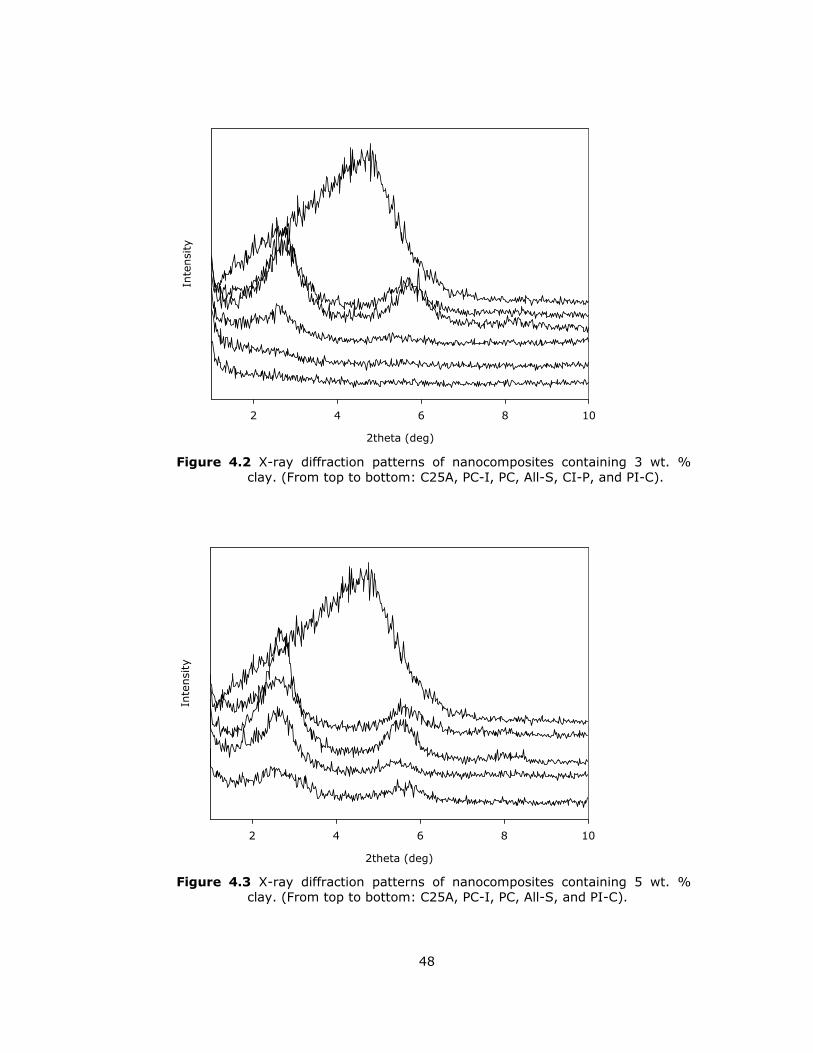
48

2theta (deg)

2 4 6 8 10

Inte

nsi

ty

Figure 4.2 X-ray diffraction patterns of nanocomposites containing 3 wt. % clay. (From top to bottom: C25A, PC-I, PC, All-S, CI-P, and PI-C).

2theta (deg)

2 4 6 8 10

Inte

nsi

ty

Figure 4.3 X-ray diffraction patterns of nanocomposites containing 5 wt. % clay. (From top to bottom: C25A, PC-I, PC, All-S, and PI-C).

49

Figures 4.1 through 4.3 show that, after melt blending, the intensity of

the diffraction peak corresponding to C25A is reduced while a set of new peaks

appear. In Figure 4.2, PC-I, PC, and All-S patterns contain diffraction peaks

characteristic of the intercalated structure. Whereas, CI-P and PI-C represent an

exfoliated structure since the peaks decrease in height and get broader as

delamination increases (Dennis et al., 2001). In other words, the polymer that

enters the galleries pushes the platelets far enough apart so that the platelets

may not be parallel to each other indicating an exfoliated structure and the

irregular platelet separation exceeds the sensitivity of X-ray diffraction. Thus, no

peak is detected by XRD.

It is apparent in Figure 4.3 that, the X-ray diffraction pattern of PI-C is

almost featureless compared with the others, only exhibiting a very broad,

extremely weak reflection at approximately 2θ of 2.47°.

50

2theta (deg)

2 4 6 8 10

Inte

nsi

ty

Figure 4.4 X-ray diffraction patterns of PET/clay nanocomposites with different clay concentrations.

Figure 4.4 shows X-ray diffraction patterns for PET/clay nanocomposites

at varying clay concentrations.

The intensity of diffraction peaks increases as a function of the clay

concentration. This indicates more ordered structures in the nanocomposites at

higher clay concentrations. At low clay concentration, part of the stacking

structure is disrupted by the imposed shear stress during the melt blending

(Xianbo and Lesser, 2003). More stacking structure was observed when the clay

concentration was higher. To conclude, exfoliated structures are observed for

addition orders designated as PI-C, CI-P and All-S. In all these cases, clay layers

are subjected to high shear stresses since the shear stress is proportional to the

viscosity at constant shear rate. Additionally, melt flow index values of the

formulations will be given in Section 4.2, supporting this explanation.

5 wt.%

3 wt.%

1 wt.%

51

4.1.2 Scanning Electron Microscopy (SEM) Analysis

There are several techniques that can be applied to evaluate the

morphology of polymer blends, SEM plays an important part for a better

understanding of the surface. In this study, both polymer matrix nanocomposites

and polymer blends are focused on since newly developed material is composed

of the three components: PET, impact modifier (E-MA-GMA) and clay (C25A). It

is known that the two polymers used in this study form a polymer blend. For

this reason, SEM was chosen to interpret the morphology regarding the

compatibility between PET and E-MA-GMA. SEM images of fractured surfaces of

all the formulations will be presented here with the same magnifications of x250

and x3500. The hair indicated at these magnifications corresponds to 100 µm

and 10 µm respectively.

Figure 4.5 represents the impact fractured surfaces of twice extruded PET

at magnifications of x250 and x3500, respectively. PET has a smooth structure.

Almost no fragmentation is observed and few straight crack lines are apparently

seen indicating low impact strength.

In Figures 4.6 and 4.7, SEM micrographs of PET/E-MA-GMA blends with

varying E-MA-GMA concentrations are shown at magnifications of x250 and

x3500, respectively. It is obvious that featureless structure of pure PET

disappears when melt blended with E-MA-GMA. In Figures 4.6 (a) and 4.6 (b),

the continuous and interpenetrated phases of PET and E-MA-GMA are clearly

seen. This suggests that there is a very good adhesion between PET and E-MA-

GMA and it is a result of intermolecular reactions between the two polymers.

Figures 4.6 (c), 4.6 (d), and 4.7 show that, at higher concentrations of

the impact modifier, the morphology is similar. The point is that E-MA-GMA is an

elastomeric material, which reduces the effective area bearing the tensile load.

Elastomers may also create cavitation which is a major mechanism of stress

relief. It is observed that, from 5 wt. % through 20 wt. % E-MA-GMA

concentrations, cavitations become larger, which alleviate the triaxial stresses

causing the cracks to grow (Sperling, 1997). Additionally, in order to observe the

morphology easily, techniques like etching by acids, swelling by solvents and

dissolving out one or the other component could have been used.

52

Figure 4.5 SEM micrographs of double extruded, pure PET with magnifications: (a) x250; (b) x3500.

Figure 4.6 SEM micrographs of PET/E-MA-GMA blends with different E-MA-GMA concentrations: (a) 5 wt. %, x250; (b) 5 wt. %, x3500; (c) 10 wt. %, x250; (d) 10 wt. %, x3500.

(a) (b)

(a) (b)

(c) (d)

53

Figure 4.7 SEM micrographs of PET/E-MA-GMA blends with different E-MA-GMA concentrations: (a) 15 wt. %, x250; (b) 15 wt. %, x3500; (c) 20 wt. %, x250; (d) 20 wt. %, x3500.

(a) (b)

(c) (d)

54

Figure 4.8 SEM micrographs of PET/E-MA-GMA/C25A nanocomposites: (a) CI-P

with 1 wt. % C25A, x250; (b) CI-P with 1 wt. % C25A, x3500; (c) CI-P with 3 wt. % C25A, x250; (d) CI-P with 3 wt. % C25A, x3500.

Figure 4.8 through 4.12 represent SEM micrographs of ternary

nanocomposites prepared by different addition orders. When the blend has tough

behavior, cavitation and extensive deformation of the matrix occur (Chapleau,

2003). However, it is very difficult to interpret the morphology of the

nanocomposites based on the effect of clay. The influence of clay concentration

looks almost the same in all of the images. For this reason, other electron

microscopy techniques such as Transmission electron microscopy (TEM), which

have higher resolution, should be utilized. In the previous section, whether the

clay is intercalated or exfoliated was discussed in light of X-ray diffraction

analysis. However, it should be supported by TEM since the features of the local

microstructure from TEM give useful detail to understand the overall picture

which is supported by XRD results.

(a) (b)

(c) (d)

55

Figure 4.9 SEM micrographs of PET/E-MA-GMA/C25A nanocomposites: (a) PC-I with 1 wt. % C25A, x250; (b) PC-I with 1 wt. % C25A, x3500; (c) PC-I with 3 wt. % C25A, x250; (d) PC-I with 3 wt. % C25A, x3500; (e) PC-I with 5 wt. % C25A, x250; (f) PC-I with 5 wt. % C25A, x3500.

(a) (b)

(c) (d)

(e) (f)

56

Figure 4.10 SEM micrographs of PET/E-MA-GMA/C25A nanocomposites: (a) PI-

C with 1 wt. % C25A, x250; (b) PI-C with 1 wt. % C25A, x3500; (c) PI-C with 3 wt. % C25A, x250; (d) PI-C with 3 wt. % C25A, x3500; (e) PI-C with 5 wt. % C25A, x250; (f) PI-C with 5 wt. % C25A, x3500.

(e) (f)

(c) (d)

(a) (b)

57

Figure 4.11 SEM micrographs of PET/E-MA-GMA/C25A nanocomposites: (a) All-

S with 1 wt. % C25A, x250; (b) All-S with 1 wt. % C25A, x3500; (c) All-S with 3 wt. % C25A, x250; (d) All-S with 3 wt. % C25A, x3500; (e) All-S with 5 wt. % C25A, x250; (f) All-S with 5 wt. % C25A, x3500.

(e) (f)

(c) (d)

(a) (b)

58

Figure 4.12 SEM micrographs of binary PET/C25A nanocomposites with

different clay concentrations: (a) 1 wt. % C25A, x250; (b) 1 wt. % C25A, x3500; (c) 3 wt. % C25A, x250; (d) 3 wt. % C25A, x3500; (e) 5 wt. % C25A, x250; (f) 5 wt. % C25A, x3500.

(e) (f)

(c) (d)

(a) (b)

59

4.2 Flow Characteristics

Melt flow index measurements were carried out under a specified load of

2.16 kg and at a specified temperature of 260°C. As is known, melt flow index is

inversely related to the melt viscosity. Additionally, the melt viscosity is related

to the molecular weight of the material. In Table 4.2, melt flow index values of

all the formulations are given.

At the end of the analysis, the followings are observed: (a) The MFI of pure PET increases (i.e. the viscosity decreases) upon extrusion

indicating chain scission.

(b) The MFI of E-MA-GMA is much lower than that of PET under the same load

and at the same temperature. Thus, in PI blends; as the impact modifier content

increases, the MFI decreases.

(c) Clay decreases the MFI (increases the viscosity) since it acts as a filler, as

observed from PC materials.

(d) Upon addition of E-MA-GMA to PC blends, the MFI decreases (the viscosity

increases) as expected. However, this decrease in MFI is not the same for all the

mixing sequences. CI-P and PI-C give the lowest MFI (highest viscosity). It

should be noted that these sequences gave rise to exfoliated structures.

In the case of PI-C, the epoxy functionality of GMA reacts with PET and

forms a viscous mixture. Thus, high shear stresses are applied on the clay layers

and exfoliation takes place. Likewise, in the case of CI-P, E-MA-GMA with high

viscosity also exfoliates the clay layers in the same manner. However, in PC-I,

this mechanism does not take place. The pure PET can not exfoliate the clay

layers.

60

Table 4.2 MFI values of all formulations.

Pure PET (not extruded) MFI (g/10 min)

610

Impact Modifier (E-MA-GMA) MFI (g/10 min)

26

PI

Impact Modifier (wt. %) MFI (g/10 min)

5 166

10 147

15 143

20 61

PC

Clay (wt. %) MFI (g/10 min)

0 809

1 496

3 358

5 262

CI-P


1 140

3 124

PC-I


1 236

3 207

5 184

PI-C


1 115

3 112

5 110

All-S


1 214

3 183

5 167

61

4.3 Mechanical Behavior

4.3.1 Effect of Impact Modifier

In order to optimize impact modifier (E-MA-GMA) content for ternary

nanocomposites composed of PET, impact modifier, and clay; mechanical

behavior of binary PET/E-MA-GMA blends was studied. At the end, the impact

modifier content providing balanced mechanical properties was determined.

Figure 4.13 presents typical stress-strain curves for pure PET and for

impact modified PET blends at various impact modifier contents. Pure PET shows

brittle behavior and fractures at about 5% strain. In contrast, all PET/impact

modifier blends are ductile with the formation of a stable neck propagating along

the gauge section before fracturing. It should be noted that pure E-MA-GMA has

a reported strain at break of 1100%.

As is seen in Figure 4.13, the stress-strain curves for impact modified PET

blends show well-defined yield points. Since the area under the curve is a

measure of the energy required to break the material, it is obvious that the

energy to fracture in stress-strain increases with increasing the modifier content.

Besides, the addition of the modifier decreases the tensile stress at yield. The

elongation at break increases significantly, jumping from 5% for pure PET to

between 100 and 300% for the modified PET, depending on the modifier

concentration.

Young's modulus values of PET/impact modifier blends are shown as a

function of impact modifier content in Figure 4.14. Pure E-MA-GMA has a

reported Young's Modulus of 8 MPa. Young's Modulus decreases from 1155 MPa

for not extruded, pure PET to nearly 600 MPa for PET containing 20 wt. % impact

modifier. Use of 5 wt. % modifier leads to a Young's modulus of 910 MPa. On the

other hand, PET at 5 wt. % loading level of impact modifier leads to lower

elongation at break compared with the ones containing 10, 15, and 20 wt. %

modifier. Percent tensile strain at break values of these blends are shown in

Figure 4.15. As a conclusion, the lower impact modifier content of PET blends

possibly explains the higher modulus and the lower elongation at break for these

blends.

62

Strain (%)

0 5 10 15 20 50 100 150 200 250 300

Str

ess

(MPa)

0

10

20

30

40

50

60

Figure 4.13 The stress-strain curves for PET (P) containing different amounts of

impact modifier (I). (From top to bottom: ( ) pure P, ( ) PI with 5 wt. %, ( ) PI with 10 wt. %, ( ) PI with 15 wt. %, ( ) PI with 20 wt. % impact modifier content.

Impact Modifier (wt. %)

0 5 10 15 20

Young's

Modulu

s (M

Pa)

500

600

700

800

900

1000

1100

1200

1300

Figure 4.14 Young's modulus values of PET/impact modifier blends as a function

of the impact modifier content.

63


0 5 10 15 20

Ten

sile

Str

ain a

t Bre

ak (

%)

0

50

100

150

200

250

300

Figure 4.15 Tensile strain at break values of PET/impact modifier blends as a

function of the impact modifier content.


0 5 10 15 20

Ten

sile

Str

ess

(MPa)

25

30

35

40

45

50

Figure 4.16 Tensile stress values of PET/impact modifier blends as a function of

the impact modifier content. (●); tensile stress at yield, (▲); tensile strength.

64


0 5 10 15 20

Flex

ura

l M

odulu

s (M

Pa)

800

1000

1200

1400

1600

1800

2000

2200

2400

Flex

ura

l Str

ength

(M

Pa)

35

40

45

50

55

60

65

70

75

Figure 4.17 Flexural strength and flexural modulus values of PET/impact

modifier blends as a function of the impact modifier content.

Tensile stress at yield and tensile strength of all investigated PET/impact

modifier blends are reported in Figure 4.16. Since there is no yield point in the

stress-strain curve for pure PET, PET has only tensile strength value at fracture,

which is the highest stress value in Figure 4.16. At 5 wt. % E-MA-GMA content,

the tensile stress at yield also gives the tensile strength of the material. The

tensile strength and tensile stress at yield decrease relatively linearly with the

impact modifier content. The property reduction is the expected result owing to

the lower strength of the modifier, reported as 4 MPa.

Figure 4.17 shows flexural strength and flexural modulus values for

PET/impact modifier blends with varying impact modifier concentration. As the

modifier concentration increases, flexural strength values and flexural moduli for

blends decrease in a similar fashion. It is apparently seen that both flexural

strength and flexural modulus values are greater than those of tensile testing.

The reason is that in flexural testing, the lower half of the specimen is in tension

and the upper half is in compression.

65

Besides, cracks do not play such an important role in compression than in

tension because the stresses tend to close the cracks rather than open them

(Nielsen and Landel, 1994).

4.3.2 Effects of Addition Order and Clay Concentration

After the impact modifier concentration was chosen as 5 wt. % owing to

its balanced mechanical properties, the effects of different addition orders and

clay concentrations on mechanical properties were investigated.

Figure 4.18 shows the typical stress-strain curves of PC nanocomposites

in the absence of impact modifier. Figures 4.19 through 4.22 illustrate the

stress-strain curves for PET/impact modifier/clay nanocomposites prepared by

different addition sequences.

For the sake of reminding, the addition orders investigated can be

summarized as follows: P, I and C stand for PET, Impact Modifier (E-MA-GMA),

and Clay respectively. The first two letters indicate the materials mixed in the

first run. This mixture was compounded with the third ingredient in the

subsequent run. The following sequences were prepared:

Sequence 1 (PI-C),

Sequence 2 (PC-I),

Sequence 3 (CI-P),

Sequence 4 (All-S) All simultaneous feeding.

66

Strain (%)

0 2 4 6 8 10

Str

ess

(MPa)

0

10

20

30

40

50

60

Figure 4.18 The stress-strain curves of PET/clay (PC) nanocomposites

containing different amounts of clay. ( ) PC with 1 wt. %; ( ) PC with 3 wt. %; (----) PC with 5 wt. % clay.

Strain (%)

0 5 10 15 20 50 100 150 200 250 300

Str

ess

(MPa)

0

10

20

30

40

50

Figure 4.19 The stress-strain curves of PET/impact modifier/clay (PI-C)

nanocomposites containing different amounts of clay. ( ) PI-C with 1 wt. %; ( ) PI-C with 3 wt. %; (----) PI-C with 5 wt. % clay.

break

67

Strain (%)

0 5 10 15 20 40 45 50 55 60

Str

ess

(MPa)

0

10

20

30

40

50

Figure 4.20 The stress-strain curves of PET/impact modifier/clay (PC-I)

nanocomposites containing different amounts of clay. ( ) PC-I with 1 wt. %; ( ) PC-I with 3 wt. %; (----) PC-I with 5 wt. % clay.

Strain (%)

0 5 10 15 20 100 150 200 250 300

Str

ess

(MPa)

0

10

20

30

40

50

Figure 4.21 The stress-strain curves of PET/impact modifier/clay (CI-P)

nanocomposites containing different amounts of clay. ( ) CI-P with 1 wt. %; ( ) CI-P with 3 wt. % clay.

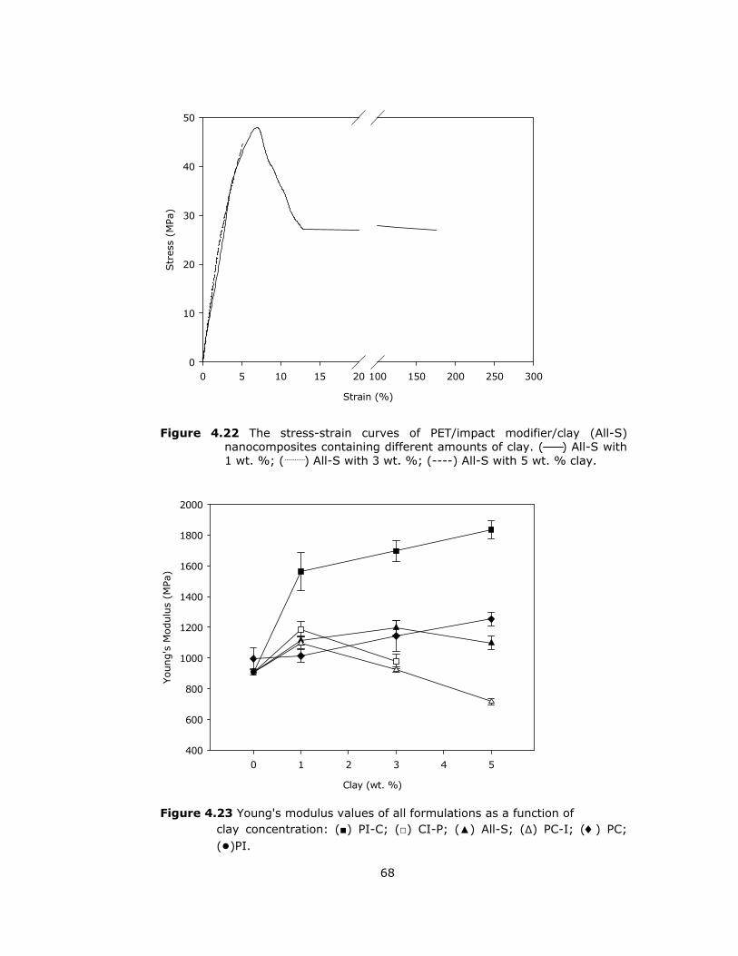
68

Strain (%)

0 5 10 15 20 100 150 200 250 300

Str

ess

(MPa)

0

10

20

30

40

50

Figure 4.22 The stress-strain curves of PET/impact modifier/clay (All-S) nanocomposites containing different amounts of clay. ( ) All-S with 1 wt. %; ( ) All-S with 3 wt. %; (----) All-S with 5 wt. % clay.

Clay (wt. %)

0 1 2 3 4 5

You

ng's

Modulu

s (M

Pa)

400

600

800

1000

1200

1400

1600

1800

2000

Figure 4.23 Young's modulus values of all formulations as a function of

clay concentration: (■) PI-C; (□) CI-P; (▲) All-S; (∆) PC-I; (♦) PC; (●)PI.

69

Figure 4.23 displays Young's Modulus values of both binary and ternary

nanocomposites with respect to the amount of clay. It is seen from Figures 4.18

through 4.23 that, Young's modulus is greatly influenced by the content of clay

and by the addition sequence of the three components.

In these figures, the characteristic behavior of polymer/layered silicate

nanocomposite materials is observed (Alexandre and Dubois, 2000). Obviously,

Young's Modulus of PET/organoclay nanocomposites (PC) increases with

increasing clay content since any filler whose modulus is greater than that of the

polymer increases the modulus of a mixture with that polymer.

For PI-C; there is a sharp increase of Young's modulus for very small clay

loadings (1 wt. %) followed by a much slower increase beyond 5 wt. % loading.

On the other hand, with increasing clay content, Young's modulus values of All-

S, CI-P, and PC-I do not change markedly up to loading levels of 3 wt. % clay

when compared with Young's modulus of PI (0 wt. % clay). These observations

support the fact that better dispersion of the clay in PET and strong interaction

between PET and the clay are essential for achieving higher Young's modulus.

In other words, as the polymer/clay adhesion is improved -as for example

when the functional groups of the impact modifier (terpolymer), which can react

with groups on the filler surface, are incorporated in the matrix- the stresses are

much more effectively transferred from the polymer matrix to the inorganic filler,

and thus a higher increase in Young's modulus is expected (Manias et al., 2001).

For this reason, compared to binary PET/clay nanocomposites (PC), ternary

PET/clay/impact modifier nanocomposites are characterized by larger modulus

increases for the same clay loading. In addition, E-MA-GMA acts as a chain

extender for PET.

Based on Young's modulus, PI-C is the best addition sequence at which

PET was first compounded with the modifier. Later, this mixture was

compounded with the clay in the subsequent run. The modification of the PET

prior to compounding with the clay may have resulted in promoting the

exfoliation of clay layers owing to the high molecular weight obtained in

comparison to pure PET.

70

While the highest Young's modulus is revealed at 5 wt.% clay for PI-C,

the lowest value obtained is at 5 wt. % clay loading for PC-I.

Clay (wt. %)

0 1 3 5

Ten

sile

Str

ength

(M

Pa)

25

30

35

40

45

50

55

60

Figure 4.24 Tensile strength as a fuction of clay content. P, PI, CI-P, PI-C, All-S, PC-I, PC.

Clay (wt. %)

0 1 3 5

Ten

sile

Str

ain a

t Bre

ak (

%)

0

50

100

150

200

250

300

Figure 4.25 Tensile strain at break (%) as a function of clay content. P, PI, CI-P, PI-C, All-S, PC-I, PC.

71

Figures 4.24 and 4.25 exhibit the tensile strength and the tensile strain at

break of the materials studied. It is observed that addition of E-MA-GMA

decreases the tensile strength of the pure PET and PET-clay binary

nanocomposite materials, since E-MA-GMA has a lower tensile strength than that

of PET. The order of the addition does not significantly affect the tensile strength

of the nanocomposites. In general, the tensile strength values of the materials

with 1 wt. % and 3 wt. % clay contents are higher than those of the materials

with 5 wt. % clay content. This is probably due to higher levels of exfoliation as

observed by XRD.

The tensile strain at break values, on the other hand, are significantly

higher at 1 wt. % clay content owing to high levels of exfoliation. While pure PET

does not show yielding and breaks at very low strains, addition of E-MA-GMA

results in a ductile material that elongates to very high extension after the yield

point. At 1 wt. % clay content, the mixing sequences of CI-P, PI-C, and to a

degree All-S exhibit yielding followed by elongation to very high strains. As

observed earlier, these mixing orders have exfoliated structure. At higher clay

content (3 wt. %), materials mixed with these sequences still exhibit yield, but

do not elongate to high strains owing to the stress concentration effect of

unexfoliated clay particles. The strain at break further decreases at 5 wt. % clay

concentration.

Figure 4.26 confirms the previous discussion. At 0 wt. % clay content,

pure PET does not exhibit yielding whereas PET/E-MA-GMA does. At 1 wt. % clay

content, PI-C, CI-P, All-S, and PC-I mixing sequences show yielding. At 3 wt. %

clay content, PI-C, CI-P and All-S mixing sequences also exhibit yielding. The

level of yield stress, when yielding exists, is insensitive to the mixing order and

the clay content. However, at the amount of 5 wt. % clay content, the

nanocomposites break without yielding.

72

Clay (wt. %)

0 1 3 5

Ten

sile

Str

ess

at Y

ield

(M

Pa)

0

10

20

30

40

50

Figure 4.26 Tensile stress at yield as a function of clay content.

Clay (wt. %)

0 1 3 5

Impac

t Str

ength

(kJ

/m2)

0

50

100

150

200

250

Figure 4.27 Impact strength as a function of clay content. P, PI, CI-P, PI-C, All-S, PC-I, PC.

PI, PI-C, CI-P, All-S, PC-I.

No y

ield

> 2

54 k

J/m

2

no break

73

The unnotched charpy impact strengths of all the materials at room

temperature are summarized in Figure 4.27. The pristine PET has a poor impact

resistance with a value of nearly 20 kJ/m2. Adding 5 wt. % impact modifier did

not significantly change the impact strength of pure PET, whereas the impact

strength results drastically changed when the modifier was added as a third

component in the PET/clay nanocomposites.

It should be noted that while pure PET specimens always broke

completely upon impact, the tough nanocomposites indicated in Figure 4.27 did

not break, and their impact strength is recorded in excess of 254 kJ/m2. The

impact values are consistent with the presence or absence of yielding. At 0 wt.

% clay content, the impact strength of the PET increases with the addition of E-

MA-GMA. At 1 wt. % clay content, the exfoliated structures of CI-P, PI-C and All-

S mixing sequences did not break and thus, their impact strength is higher than

254 kJ/m2. At 3 wt. % clay content, the same is true for the PI-C mixing order.

The impact strength values of the materials with CI-P and All-S mixing

sequences are still high. The impact strength decreases at 5 wt. % clay content

owing to the stress concentration effect of unexfoliated clay.

Based on the impact and the strain at break results, the best sequence of

component addition is once more selected as (PI-C). In this case, the polymer

matrix mixture prepared in the first run (PI) has higher melt viscosity than does

pure PET as observed by MFI. Thus this matrix can apply high shear stresses on

the clay particles and delaminate the clay layers resulting in best mechanical

properties. However, in other addition sequences such as PC-I, the matrix can

not apply high shear stresses owing to its lower viscosity.

74

Clay (wt. %)

0 1 2 3 4 5

Flex

ura

l M

odulu

s (M

Pa)

1600

1800

2000

2200

2400

2600

2800

Figure 4.28 Flexural modulus as a function of clay content:

(■) PI-C; (□)CI-P; (▲) All-S; (∆) PC-I; (♦) PC; (●) PI.

Clay (wt. %)

0 1 2 3 4 5

Flex

ura

l Str

ength

(M

Pa)

50

55

60

65

70

75

80

Figure 4.29 Flexural strength as a function of clay content:

(■) PI-C; (□) CI-P; (▲) All-S; (∆) PC-I; (♦) PC; (●) PI.

75

The flexural modulus and strength values are shown in Figures 4.28 and

4.29 respectively. Generally speaking, the flexural modulus increases with the

addition of rigid clay particles. E-MA-GMA decreases the modulus, since it is a

rubbery material. Thus, PC binary nanocomposites have the highest modulus in

general. The flexural modulus is not sensitive to the mixing order. It is the

components and their contents which are effective in determining the modulus,

as implied by several theories on modulus (Nielsen and Landel, 1994).

The level of flexural modulus is significantly higher than the tensile

modulus due to the nature of the flexural test as observed in other composites.

Flexural strength is not significantly affected by the mixing sequence and the

clay content studied here. The PC nanocomposites exhibit the highest level of

flexural strength owing to the lack of E-MA-GMA with low strength. The flexural

strength is also higher than the tensile strength, since in flexural test the cracks

formed can not propagate easily towards the upper part of the specimen which is

in compression.

Lastly, in flexural testing break point was observed only on the PC

nanocomposites with 5 wt. % clay content, and the PC-I ternary nanocomposites

with 5 wt. % clay content owing to the extensibility imparted by E-MA-GMA.

Flexural strain at break (%) values of these materials are nearly 5% and 6%

respectively.

76

4.4 Thermal Analysis

Poly(ethylene terephthalate) used in this study, has a glass transition

temperature (Tg) at 76.7°C, a melting temperature (Tm) at 253.9°C with an

onset temperature of 235.6°C, and a crystallization temperature at 138.7°C with

an onset temperature of 132.5°C. Generally speaking, the Tg and the Tm of

polymers containing aromatic moieties such as phenylene are high when

compared with those of polymers derived from aliphatic containing reactants

(Seymour and Carraher, 1984). The high Tg and Tm values of PET are the result

of the rigidity of the aromatic portion of the polymer. Another stiffening group

known as carboxyl group is also present in the structure of PET.

On the other hand, the glass transition temperature of the impact

modifier is below the room temperature. For this reason, it was not detected by

DSC analysis. The impact modifier (E-MA-GMA) is a semi-crystalline terpolymer

with a melting temperature of 68.8°C. Because of the irregularity in its structure,

the Tm of E-MA-GMA is lower than the Tm of either of the homopolymers.

As is seen in Table 4.3, the melting temperature (Tm) and the glass

transition temperature (Tg) of all the formulations remain almost the same, the

variations are about 2-4°C. This suggests that the incorporation of both clay and

impact modifier do not influence much the melting and glass transition behavior

of the compositions. However, the highest Tg values are observed for PI-C with

1 wt. % and 3 wt. % clay and All-S with 1 wt. % clay concentration, which are

79.4°C, 79.7°C, and 79.5°C respectively. It is obvious that relative to the pure

PET, the composites containing exfoliated clay show higher Tg. This finding

suggests that PET segments confined within the silicate galleries of the clay tend

to retard the segmental motion of the PET matrix (Tseng et al., 2002).

As for the crystallization temperature (Tc); all compositions show

crystallization peak during heating and the crystallization temperature during

heating process decreases by the addition of the clay and impact modifier. For

example, the Tc values of PI-C with 1 wt. %, 3 wt. %, and 5 wt. % clay contents

are 128.5°C, 122.4°C, and 118.7°C respectively. It is apparent that Tc of PI-C

with 1 wt. % clay concentration is about 10°C lower than that of pure PET. The

effect of clay content on the crystallization temperature (Tc) for all the

formulations can clearly be seen in Table 4.3. The influence of addition order on

crystallization temperature is not significant as compared with the effect of clay

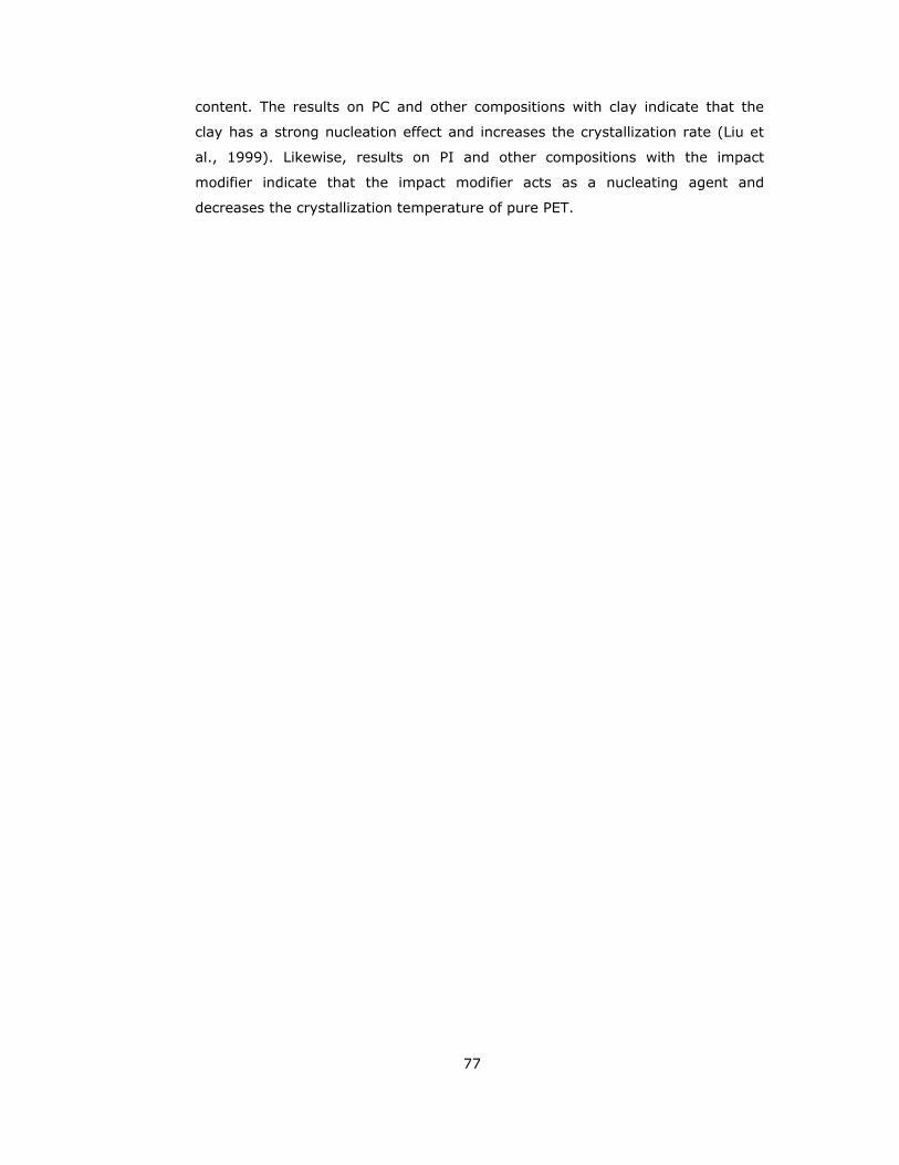
77

content. The results on PC and other compositions with clay indicate that the

clay has a strong nucleation effect and increases the crystallization rate (Liu et

al., 1999). Likewise, results on PI and other compositions with the impact

modifier indicate that the impact modifier acts as a nucleating agent and

decreases the crystallization temperature of pure PET.

78

Table 4.3 Thermal properties of all formulations.

Pure PET (not extruded) Tg(°C) Tc(°C) Tm(°C)

76.7 138.7 253.9

Impact Modifier (E-MA-GMA)

<20 - 68.8

PI

Impact Modifier (wt. %) Tg(°C) Tc(°C) Tm(°C)

5 76.5 126.3 255.5

10 76.3 130.6 255.1

15 77.7 129.0 254.3

20 78.8 126.2 254.3

PC

Clay (wt. %) Tg(°C) Tc(°C) Tm(°C)

0 77.5 133.8 255.6

1 78.8 120.6 256.3

3 78.5 121.9 256.1

5 76.9 116.1 253.8

CI-P


1 74.6 130.4 254.9

3 78.1 121.0 253.9

PC-I


1 77.8 126.0 257.3

3 74.6 119.4 253.9

5 76.9 116.4 255.5

PI-C


1 79.4 128.5 253.8

3 79.7 122.4 255.1

5 73.6 118.7 253.9

All-S


1 79.5 126.6 257.4

3 74.8 123.6 254.8

5 78.3 122.1 256.0

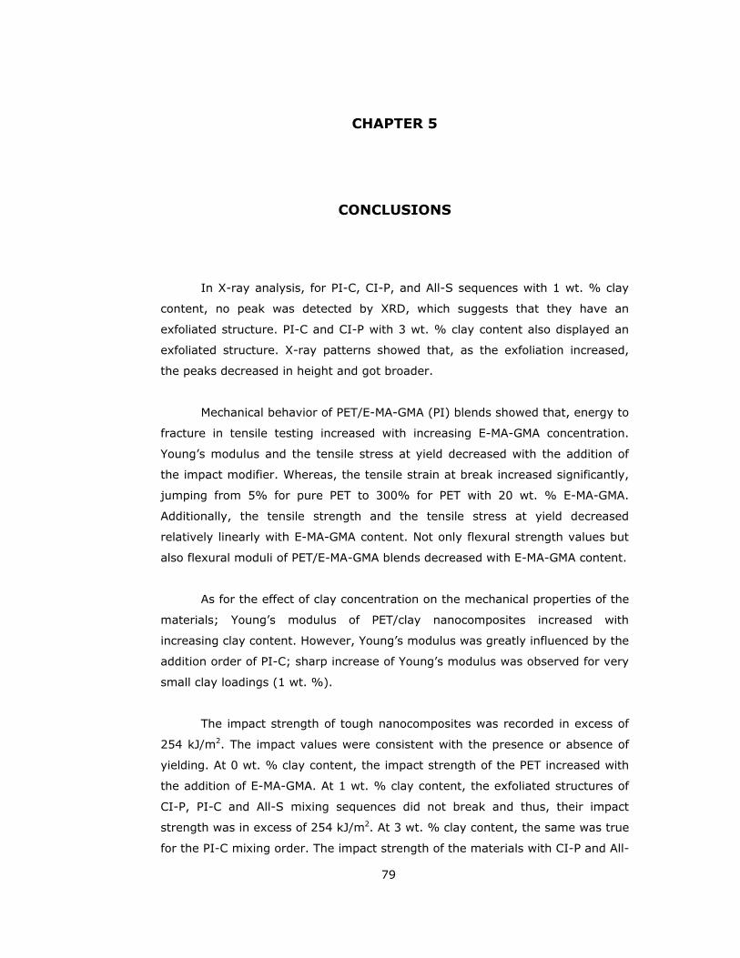
79

CHAPTER 5

CONCLUSIONS

In X-ray analysis, for PI-C, CI-P, and All-S sequences with 1 wt. % clay

content, no peak was detected by XRD, which suggests that they have an

exfoliated structure. PI-C and CI-P with 3 wt. % clay content also displayed an

exfoliated structure. X-ray patterns showed that, as the exfoliation increased,

the peaks decreased in height and got broader.

Mechanical behavior of PET/E-MA-GMA (PI) blends showed that, energy to

fracture in tensile testing increased with increasing E-MA-GMA concentration.

Young’s modulus and the tensile stress at yield decreased with the addition of

the impact modifier. Whereas, the tensile strain at break increased significantly,

jumping from 5% for pure PET to 300% for PET with 20 wt. % E-MA-GMA.

Additionally, the tensile strength and the tensile stress at yield decreased

relatively linearly with E-MA-GMA content. Not only flexural strength values but

also flexural moduli of PET/E-MA-GMA blends decreased with E-MA-GMA content.

As for the effect of clay concentration on the mechanical properties of the

materials; Young’s modulus of PET/clay nanocomposites increased with

increasing clay content. However, Young’s modulus was greatly influenced by the

addition order of PI-C; sharp increase of Young’s modulus was observed for very

small clay loadings (1 wt. %).

The impact strength of tough nanocomposites was recorded in excess of

254 kJ/m2. The impact values were consistent with the presence or absence of

yielding. At 0 wt. % clay content, the impact strength of the PET increased with

the addition of E-MA-GMA. At 1 wt. % clay content, the exfoliated structures of

CI-P, PI-C and All-S mixing sequences did not break and thus, their impact

strength was in excess of 254 kJ/m2. At 3 wt. % clay content, the same was true

for the PI-C mixing order. The impact strength of the materials with CI-P and All-

80

S mixing sequences was still high. However, the impact strength decreased at 5

wt. % clay content.

The tensile strain at break values, on the other hand, were significantly

higher at 1 wt. % clay content. While pure PET did not show yielding and

fractured at very low strain values, addition of E-MA-GMA resulted in a ductile

material that extended to a very high strain after the yield point. At 1 wt. % clay

content, the mixing sequences of CI-P, PI-C, and to a degree All-S exhibited

yielding followed by elongation to very high strains.

In SEM micrographs, smooth structure of pure PET disappeared when

melt blended with E-MA-GMA. The influence of clay concentration looked almost

the same in all of the images.

MFI measurements showed that, the MFI of pure PET increased upon

extrusion. The MFI of E-MA-GMA was much lower than that of PET under the

same load and at the same temperature. Thus, in PI blends; as the impact

modifier content increased, the MFI decreased. In addition, clay decreased the

MFI of the compositions. Upon addition of E-MA-GMA to PC blends, the MFI

decreased. However, this decrease in MFI was not the same for all the mixing

sequences. CI-P and PI-C gave the lowest MFI (highest viscosity).

DSC analysis showed that, the melting temperature (Tm) and the glass

transition temperature (Tg) of all formulations remained almost the same. This

implied that the incorporation of both clay and impact modifier did not

significantly affect the melting and glass transition behavior of the compositions.

However, the highest Tg values were observed for PI-C with 1 wt. % and 3 wt.

% clay and All-S with 1 wt. % clay concentration, which suggested that relative

to pure PET, the composites containing exfoliated clay showed higher Tg. The

crystallization temperature during heating process decreased by the addition of

the clay and impact modifier. Results on PI and other compositions with the

impact modifier indicated that, the impact modifier and clay acted as a

nucleating agent and decreased the crystallization temperature of pure PET.

81

REFERENCES

Alexandre, M., and Dubois, P., 2000. Polymer-Layered Silicate Nanocomposites: Preparation, Properties, and Uses of a New Class of Materials, Materials Science and Engineering, 28, 1-63.

ASTM D256-92, 1993. Standart Test Method for Impact Resistance of Plastics and Electrical Insulating Materials, Annual Book of ASTM Standards, 08.01, 58-74, Philadelphia, PA.

ASTM D638M-91a, 1993. Standart Test Method for Tensile Properties of Plastics, Annual Book of ASTM standards, 08.01, 174-182, Philadelphia, PA.

ASTM D790M-92, 1993. Standart Test Methods for Flexural Properties of Unreinforced and Reinforced Plastics and Electrical Insulating Materials, Annual Book of ASTM standards, 08.01, 284-292, Philadelphia, PA.

ASTM D1238-79, 1993. Standart Test Method for Flow Rates of Thermoplastics by Extrusion Plastometer, Annual Book of ASTM Standards, 08.01, 467-479, Philadelphia, PA.

Beyer, G., 2002. Nanocomposites: a New Class of Flame Retardants for Polymers, Plastics Additives and Compounding, October, 22-28.

Billmeyer, F.W., 1984. Textbook of Polymer Science, 3rd ed., John Wiley and Sons, Inc., NY.

Broutman, L.J., and Krock R.H., 1967. Modern Composite Materials, Addison-Wesley Publishing Company, MA.

Callister, W.D., 1997. Materials Science and Engineering: an Introduction, 4th ed., John Wiley and Sons, Inc., NY.

Chapleau, N., and Huneault, M.A., 2003. Impact Modification of Poly(ethylene terephthalate), Journal of Applied Polymer Science, 90, 2919-2932.

Chazeau, L., Cavaille, J.Y., Canova, G., Dendievel, R., Boutherin, B., 1999. Viscoelastic Properties of Plasticized PVC Reinforced with Cellulose Whiskers, Journal of Applied Polymer Science, 71, 1797-1808.

82

Chou, N.J., Kowalczyk, S.P., Saraf, R., Tong, H.M., 1994. Characterization of Polymers, Manning Publication, Co., CT.

Concise Encyclopedia of Polymer Science and Engineering, 1990. John Wiley and Sons, Inc., NY.

Davis, C.H., Mathias, L.J., Gilman, J.W., Schiraldi, A., Shields, J.R., Trulove, P., Sutto, T.E., Delong, H.C., 2002. Effects of Melt-Processing Conditions on the Quality of Poly(ethylene terephthalate) Montmorillonite Clay Nanocomposites, Journal of Polymer Science: Part B: Polymer Physics, 40, 2661-2666.

Dennis, H.R., Hunter, D.L., Chang, D., Kim, S., White, J.L., Cho, J.W., Paul, D.R., 2001. Effect of Melt Processing Conditions on the Extent of Exfoliation in Organoclay-Based Nanocomposites, Polymer, 42, 9513-9522.

Encyclopedia of Polymer Science and Technology, 1970. Plastics, Resins, Rubbers, and Fibers, 13, John Wiley and Sons, Inc., NY.

Favier, V., Canova, G.R., Shrivastava, S.C., Cavaille, J.Y., 1997. Mechanical Percolation in Cellulose Whiskers Nanocomposites, Polymer Engineering and Science, 37, 1732-1739.

Fisher, E.G., 1976. Extrusion of Plastics, 3rd ed., Newness-Butterworths, London.

Fukushima, Y., Okada, A., Kawasumi, M., Kurauchi, T., Kamigaito, O., 1988. Swelling Behavior of Montmorillonite by Poly-6-amide, Clay Minerals, 23, 27-34.

Giannelis, E.P., 1996. Polymer Layered Silicate Nanocomposites, Advanced Materials, 8, 29-35.

Giannelis, E.P., 1998. Polymer-Layered Silicate Nanocomposites: Synthesis, Properties and Applications, Applied Organometallic Chemistry, 12, 675-680.

Giannelis, E.P., 1999. Polymer-Layered Silicate Nanocomposites: Emerging Scientific and Commercial Opportunities, Proceedings of 57th SPE Annual Technical Conference (ANTEC), 155, 3966-3968.

Giannelis, E.P., Krishnamoorti, R., Manias, E., 1999. Polymer-Silicate Nanocomposites: Model Systems for Confined Polymers and Polymer Brushes, Advances in Polymer Science, 138, 108-147.

83

Gibson, R.F., 1994. Principles of Composite Material Mechanics. Mc-Graw Hill, Inc., NY.

Giese, R.F., and Van Oss, C.J., 2002. Colloid and Surface Properties of Clays and Related Minerals, Surfactant Science Series, 105, Marcel Dekker, Inc., NY.

Grubb, D.T., 1974. Review: Radiation Damage and Electron Microscopy of Organic Polymers, Journal of Materials Science, 9, 1715-1736.

Hasegawa, N., Okamoto, H., Kato, M., Usuki, A., 2000. Preparation and Mechanical Properties of Polypropylene-Clay Hybrids Based on Modified Polypropylene and Organophilic Clay, Journal of Applied Polymer Science, 78, 1918-1922.

Herron, N., and Thorn, D.L., 1998. Nanoparticles: Uses and Relationships to Molecular Clusters, Advanced Materials, 10, 1173-1184.

Hert, M., 1992. Tough Thermoplastic Polyesters by Reactive Extrusion with Epoxy-containing Copolymers, Die Angewandte Makromolekulare Chemie, 196, 89-99.

Imai, Y., Nishimura, S., Abe, E., Tateyama, H., Abiko, A., Yamaguchi, A., Aoyama, T., Taguchi, H., 2002. High-Modulus Poly(ethylene terephthalate)/Expandable Fluorine Mica Nanocomposites with a Novel Reactive Compatibilizer, Chemistry of Materials, 14, 477-479.

Kalfoglou, N.K., Skafidas, D.S., Kallitsis, J.K., 1995. Comparison of Compatibilizer Effectiveness for PET/HDPE Blends, Polymer, 36, 4453-4462.

Ke, Y.C., Long, C.F., Qi, Z.N., 1999. Crystallization, Properties, and Crystal and Nanoscale Morphology of PET-Clay Nanocomposites, Journal of Applied Polymer Science, 71, 1139-1146.

Kirk, R.E., and Othmer, D.F., 1995. Encyclopedia of Chemical Technology, 4th ed., John Wiley and Sons, Inc., NY.

Le Baron, P.C., Wang, Z., Pinnavaia, T.J., 1999. Polymer-Layered Silicate Nanocomposites: an Overview, Applied Clay Science, 15, 11-29.

Liu, L., Qi, Z., Zhu, X., 1999. Studies on Nylon 6/Clay Nanocomposites by Melt-Intercalation Process, Journal of Applied Polymer Science, 71, 1133-1138.

84

Lobo, H., and Bonilla, J.V., 2003. Handbook of Plastics Analysis, Marcel Dekker, Inc., NY.

Loyens, W., and Groeninckx, G., 2002a. Ultimate Mechanical Properties of Rubber Toughened Semicrystalline PET at Room Temperature, Polymer, 43, 5679-5691.

Loyens, W., and Groeninckx, G., 2002b. Phase Morphology Development in Reactively Compatibilised Polyethylene Terephthalate/Elastomer Blends, Macromolecular Chemistry and Physics, 203, 1702-1714.

Manias, E., Touny, A., Wu, L., Strawhecker, K., Lu, B., Chung, T.C., 2001. Polypropylene/Montmorillonite Nanocomposites. Review of the Synthetic Routes and Materials Properties, Chemistry of Materials, 13, 3516-3523.

Mark, J.E., 1996. Ceramic Reinforced Polymers and Polymer-Modified Ceramics, Polymer Engineering and Science, 36, 2905-2920.

Morton-Jones, D.H., 1989. Polymer Processing, Chapman and Hall, Inc., NY.

Nielsen, L.E., Landel, R.F., 1994. Mechanical Properties of Polymers and Composites, 2nd ed., Marcel Dekker, Inc., NY.

Pinnavaia, T.J., and Beall, G.W., 2000. Polymer-Clay Nanocomposites, John Wiley and Sons, Inc., Chichester, England.

Polymeric Materials Encyclopedia, 1996. Vol. 8, CRC Press, Inc., NY.

Rosen, S.L., 1993. Fundamental Principles of Polymeric Materials, 2nd ed., John Wiley and Sons, Inc., NY.

Sawyer, L.C., and Grubb, D.T., 1987. Polymer Microscopy, Chapman and Hall, Inc., NY.

Schmidt, D., Shah, D., Giannelis, E.P., 2002. New Advances in Polymer/Layered Silicate Nanocomposites, Current Opinion in Solid State and Materials Science, 6, 205-212.

Schwartz, M.M., 1997. Composite Materials: Processing, Fabrication, and Applications, Prentice-Hall, Inc., NJ.

Seymour, R.B., and Carraher, C.E., 1984. Structure-Property Relationships in Polymers, Plenum Press, NY.

85

Seymour, R.B., and Deanin, R.D., 1987. History of Polymeric Composites, Proceedings of 192nd ACS National Meeting, VNU Science Press, Utrecht, The Netherlands.

Sherman, L.M., 1999. Nanocomposites- a Little Goes a Long Way, Plastics Technology, 45, 52-57.

Sinha Ray, S., and Okamoto, M., 2003. Polymer/Layered Silicate Nanocomposites: a Review from Preparation to Processing, Progress in Polymer Science, 28, 1539-1641.

Solomons, T.W.G., 1996. Organic Chemistry, 6th ed., John Wiley and Sons, Inc., NY.

Sperling, L.H., 1997. Polymeric Multicomponent Materials, an Introduction, John Wiley and Sons, Inc., NY.

Strong, A.B., 1996. Plastics: Materials and Processing, Prentice-Hall, Inc., NJ.

Tsai, T.Y., Hwang, C.L., Lee, S.Y., 2000. A Fresh Approach of Modified Clays for Polymer/Clay Nanocomposites, Proceedings of 58th SPE Annual Technical Conference (ANTEC), 248, 2412-2415.

Tseng, C.R., Wu, J.Y., Lee, H.Y., Chang, F.C., 2002. Preparation and Characterization of Polystyrene-Clay Nanocomposites by Free-Radical Polymerization, Journal of Applied Polymer Science, 85, 1370-1377.

Ullmann's Encyclopedia of Industrial Chemistry, 1992. 5th Ed. Vol A20, VCH Publishers, NY.

Vaia, R.A., Ishii, H., Giannelis, E.P., 1993. Synthesis and Properties of Two-Dimensional Nanostructures by Direct Intercalation of Polymer Melts in Layered Silicates, Chemistry of Materials, 5, 1694-1696.

Vaia, R.A., Klaus, D.J., Kramer, E.J., 1995. Kinetics of Polymer Melt Intercalation, Macromolecules, 28, 8080-8085.

Vaia, R.A., Jandt, K.D., Kramer, E.J., Giannelis E.P., 1996. Microstructural Evolution of Melt Intercalated Polymer-Organically Modified Layered Silicates Nanocomposites, Chemistry of Materials, 8, 2628-2635.

Watson, E.S., O'Neill, M.J., Justin, J., Brenner, N., 1964. A Differential Scanning Calorimeter for Quantitative Differential Thermal Analysis, Analytical Chemistry, 36, 1233-1238.

86

Xanthos, M., and Dagli, S.S., 1991. Compatibilization of Polymer Blends by Reactive Processing, Polymer Engineering and Science, 31, 929-935.

Xianbo, H., and Lesser, A.J., 2003. Effect of a Silicate Filler on the Crystal Morphology of Poly(trimethylene terephthalate)/Clay Nanocomposites, Journal of Polymer Science: Part B: Polymer Physics, 41, 2275–2289.

Yoon, J.T., Jo, W.H., Lee, M.S., Ko, M.B., 2001. Effects of Comonomers and Shear on the Melt Intercalation of Styrenics/Clay Nanocomposites. Polymer, 42, 329-336.

87

APPENDIX A

Mechanical Testing Results

Table A.1 Arithmetic means and standard deviations of Young’s modulus values

for all formulations.

Pure PET (not extruded) Young's Modulus (MPa) Stdev

1155 19.3

PI

Impact Modifier (wt. %) Young's Modulus (MPa) Stdev

5 909 18.9

10 832 24.9

15 725 7.5

20 619 13.4

PC

Clay (wt. %) Young's Modulus (MPa) Stdev

0 994 72.0

1 1014 41.1

3 1144 100.0

5 1253 42.2

CI-P


1 1187 49.0

3 977 46.0

PC-I


1 1097 38.7

3 923 17.7

5 716 19.5

88

Table A.1 (Cont’d).

PI-C


1 1563 121.7

3 1696 65.7

5 1923 41.3

All-S


1 1113 29.3

3 1197 46.6

5 1098 44.6

89

Table A.2 Arithmetic means and standard deviations of tensile strength values


Pure PET (not extruded) Tensile Strength (MPa) Stdev

49.1 1.33

PI

Impact Modifier (wt. %) Tensile Strength (MPa) Stdev

5 43.7 0.29

10 38.6 1.11

15 36.3 1.62

20 30.3 0.82

PC

Clay (wt. %) Tensile Strength (MPa) Stdev

0 47.7 0.72

1 51.3 0.44

3 52.6 1.42

5 43.5 5.31

CI-P


1 45.5 0.73

3 42.5 0.25

PC-I


1 42.6 2.52

3 44.9 1.60

5 34.3 3.44

PI-C


1 43.7 0.08

3 46.8 0.15

5 39.4 5.34

All-S


1 47.0 0.33

3 45.0 4.41

5 46.8 1.25

90

Table A.3 Arithmetic means and standard deviations of tensile stress at yield

values for all formulations.

Pure PET (not extruded) Tensile Stress at Yield (MPa) Stdev

no yield -

PI

Impact Modifier (wt. %) Tensile Stress at Yield (MPa) Stdev

5 43.7 0.29

10 35.8 0.31

15 31.2 0.33

20 27.4 0.14

PC

Clay (wt. %) Tensile Stress at Yield (MPa) Stdev

0 no yield -

1 no yield -

3 no yield -

5 no yield -

CI-P


1 45.5 0.73

3 42.5 0.25

PC-I


1 42.6 2.52

3 44.9 1.60

5 no yield -

PI-C


1 43.7 0.08

3 46.8 0.15

5 no yield -

All-S


1 47.0 0.33

3 no yield -

5 no yield -

91

Table A.4 Arithmetic means and standard deviations of tensile strain at break

values for all formulations.

Pure PET (not extruded) Tensile Strain at Break (%) Stdev

5.7 0.59

PI

Impact Modifier (wt. %) Tensile Strain at Break (%) Stdev

5 133.1 13.73

10 226.3 12.63

15 239.5 8.66

20 264.5 17.47

PC

Clay (wt. %) Tensile Strain at Break (%) Stdev

0 4.5 0.40

1 5.4 0.55

3 7.5 0.43

5 5.8 0.51

CI-P


1 266.2 0.14

3 7.8 1.15

PC-I


1 44.0 46.21

3 12.6 3.84

5 5.4 0.81

PI-C


1 287.0 7.19

3 26.8 6.02

5 4.2 0.62

All-S


1 188.3 0.22

3 6.5 1.90

5 6.2 0.84

92

Table A.5 Arithmetic means and standard deviations of flexural modulus values


Pure PET (not extruded) Flexural Modulus (MPa) Stdev

2523 29.4

PI

Impact Modifier (wt. %) Flexural Modulus (MPa) Stdev

5 2125 51.7

10 1648 24.5

15 1420 43.3

20 1198 19.9

PC

Clay (wt. %) Flexural Modulus (MPa) Stdev

0 2202 80.8

1 2284 26.6

3 2479 49.8

5 2662 11.0

CI-P


1 1964 42.2

3 1704 11.2

PC-I


1 2223 39.6

3 2156 83.3

5 2487 92.7

PI-C


1 2109 36.6

3 2331 20.4

5 2718 29.8

All-S


1 2152 31.8

3 2264 29.0

5 2317 40.9

93

Table A.6 Arithmetic means and standard deviations of flexural strength values


Pure PET (not extruded) Flexural Strength (MPa) Stdev

77.9 1.38

PI

Impact Modifier (wt. %) Flexural Strength (MPa) Stdev

5 66.6 0.43

10 50.6 0.45

15 44.4 0.43

20 37.7 0.41

PC

Clay (wt. %) Flexural Strength (MPa) Stdev

0 67.9 1.38

1 70.4 0.55

3 73.3 1.58

5 75.7 0.77

CI-P


1 60.5 0.53

3 53.7 0.56

PC-I


1 68.3 0.53

3 62.9 0.98

5 67.6 1.30

PI-C


1 61.4 0.85

3 64.3 0.20

5 69.5 0.72

All-S


1 65.5 0.57

3 66.1 0.87

5 65.2 0.95

94

Table A.7 Arithmetic means and standard deviations of impact strength values


Pure PET (not extruded) Impact Strength (kJ/m2) Stdev

24.3 3.12

PI

Impact Modifier (wt. %) Impact Strength (kJ/m2) Stdev

5 30.5 6.15

10 no break (>254) -

15 no break (>254) -

20 no break (>254) -

PC

Clay (wt. %) Impact Strength (kJ/m2) Stdev

0 17.9 2.44

1 12.2 2.94

3 9.0 1.03

5 9.3 0.77

CI-P


1 no break (>254) -

3 43.1 3.17

PC-I


1 11 4.61

3 10.8 3.47

5 11.3 3.80

PI-C


1 no break (>254) -

3 no break (>254) -

5 26.5 2.38

All-S


1 no break (>254) -

3 78.7 4.78

5 52.3 4.76

95

APPENDIX B

DSC Thermograms

Figure B.1 DSC thermogram of not extruded, pure PET.

96

Figure B.2 DSC thermogram of impact modifier (E-MA-GMA).

Figure B.3 DSC thermogram of double extruded PET.

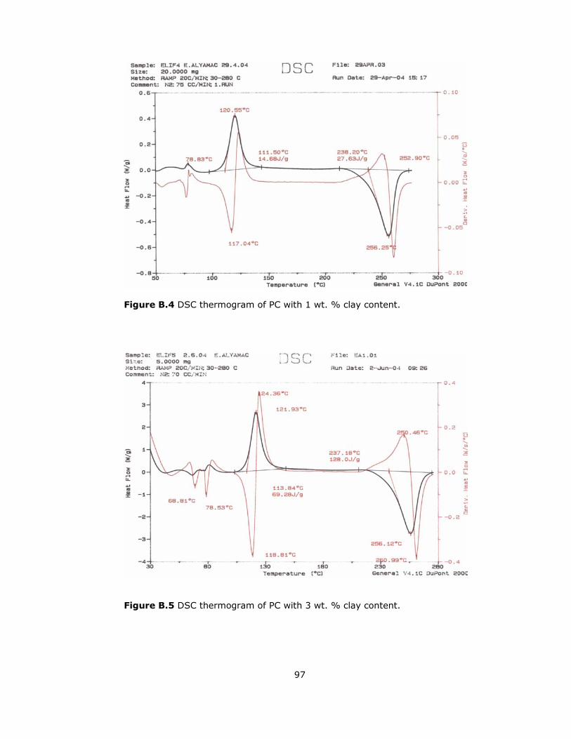
97

Figure B.4 DSC thermogram of PC with 1 wt. % clay content.


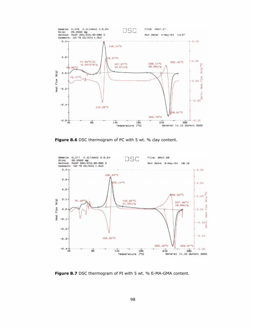
98


Figure B.7 DSC thermogram of PI with 5 wt. % E-MA-GMA content.

99



100


Figure B.11 DSC thermogram of CI-P with 1 wt. % clay content.

101

Figure B.12 DSC thermogram of CI-P with 3 wt. % clay content.

Figure B.13 DSC thermogram of PC-I with 1 wt. % clay content.

102



103

Figure B.16 DSC thermogram of PI-C with 1 wt. % clay content.


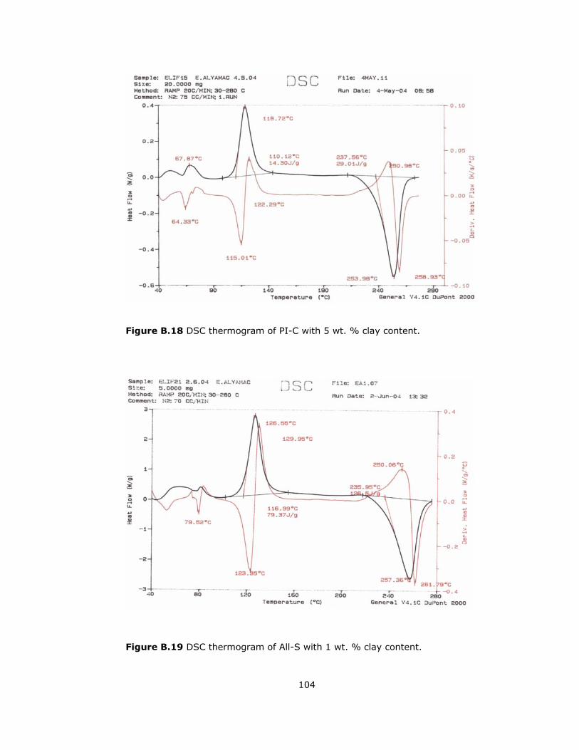
104


Figure B.19 DSC thermogram of All-S with 1 wt. % clay content.

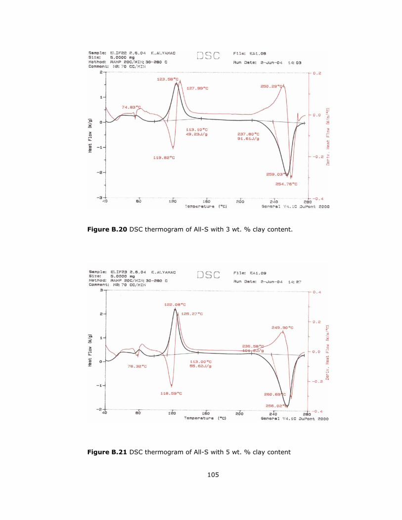
105

Figure B.20 DSC thermogram of All-S with 3 wt. % clay content.

Figure B.21 DSC thermogram of All-S with 5 wt. % clay content

106

APPENDIX C

X-Ray Diffraction Patterns

2theta (deg)

2 4 6 8 10

Inte

nsi

ty (

counts

)

0

20

40

60

80

100

120

140

160

Figure C.1 X-ray diffraction patterns of PC with 1 wt. % clay content.

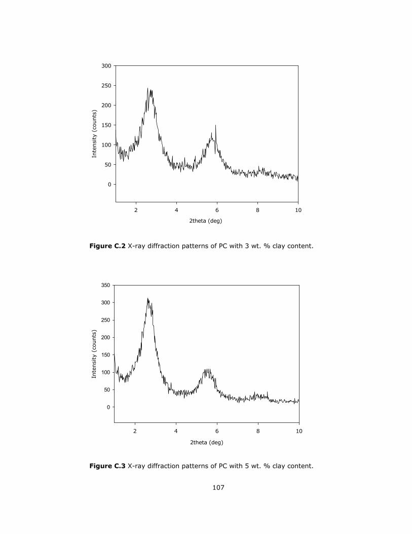
107

2theta (deg)

2 4 6 8 10

Inte

nsi

ty (

counts

)

0

50

100

150

200

250

300


2theta (deg)

2 4 6 8 10

Inte

nsi

ty (

counts

)

0

50

100

150

200

250

300

350


108

2theta (deg)

2 4 6 8 10

Inte

nsi

ty (

counts

)

0

20

40

60

80

100

120

140

160

Figure C.4 X-ray diffraction patterns of CI-P with 1 wt. % clay content.

2theta (deg)

2 4 6 8 10

Inte

nsi

ty (

counts

)

0

20

40

60

80

100

120

Figure C.5 X-ray diffraction patterns of CI-P with 3 wt. % clay content.

109

2theta (deg)

2 4 6 8 10

Inte

nsi

ty (

counts

)

0

50

100

150

200

Figure C.6 X-ray diffraction patterns of PC-I with 1 wt. % clay content.

2theta (deg)

2 4 6 8 10

Inte

nsi

ty (

counts

)

0

50

100

150

200


110

2theta (deg)

2 4 6 8 10

Inte

nsi

ty (

counts

)

0

50

100

150

200


2theta (deg)

2 4 6 8 10

Inte

nsi

ty (

counts

)

0

20

40

60

80

100

120

Figure C.9 X-ray diffraction patterns of PI-C with 1 wt. % clay content.

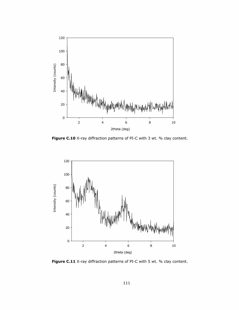
111

2theta (deg)

2 4 6 8 10

Inte

nsi

ty (

counts

)

0

20

40

60

80

100

120


2theta (deg)

2 4 6 8 10

Inte

nsi

ty (

counts

)

0

20

40

60

80

100

120


112

2theta (deg)

2 4 6 8 10

Inte

nsi

ty (

counts

)

0

20

40

60

80

100

Figure C.12 X-ray diffraction patterns of All-S with 1 wt. % clay content.

2theta (deg)

2 4 6 8 10

Inte

nsi

ty (

counts

)

0

50

100

150

200


113

2theta (deg)

2 4 6 8 10

Inte

nsi

ty (

counts

)

0

50

100

150

200


impact modified poly(ethylene terephthalate) …etd.lib.metu.edu.tr/upload/12605092/index.pdf · vi...

Documents