Impact of Connection and Automation on Electrified Vehicle Energy Consumption

SAE 2015 Vehicle Electrification and Connected Vehicle Technology ForumDecember 04, 2015

Aymeric Rousseau, Pierre Michel, Dominik KarbowskiArgonne National Laboratory

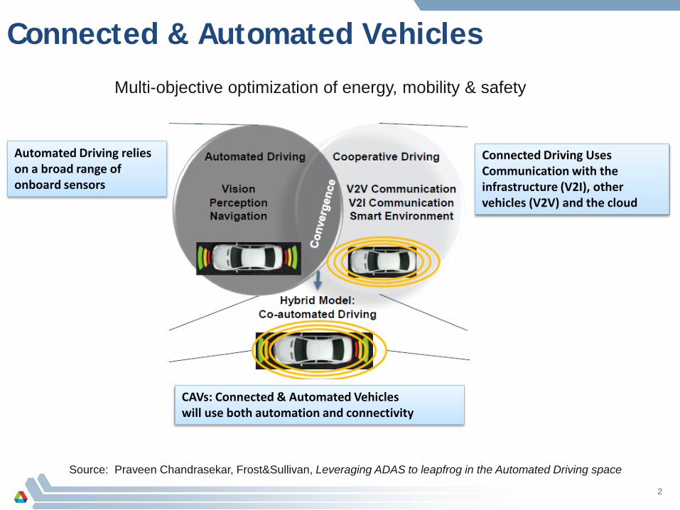
Connected & Automated Vehicles

Source: Praveen Chandrasekar, Frost&Sullivan, Leveraging ADAS to leapfrog in the Automated Driving space

Automated Driving relies on a broad range of onboard sensors

Connected Driving Uses Communication with the infrastructure (V2I), other vehicles (V2V) and the cloud

CAVs: Connected & Automated Vehicleswill use both automation and connectivity

Multi-objective optimization of energy, mobility & safety

2

Tomorrow’s Transportation Will Feature a Rich Combination of Technologies

Various powertrains Various level of vehicle automation Various ITS technologies Various levels of communication

530

HEV

EV

PHEV

Autonomous Vehicle

PlatooningEco-Approach

Adaptive Cruise Control

Variable Speed Limit

Signal Broadcasting

Dynamic light sequencing

Traffic Management

Center

V2I

V2V

3

Electric Drive Vehicles Could Benefit from CAVs Technologies from Connectivity and Automation

4

• Route Based Control would allow lower fuel consumption by optimizing electric consumption throughout a trip.

• Opportunity for optimal powertrain design and speed control• Knowing location of charging stations, their status as well as

the vehicles’ battery SOC would provide helpful information to drivers (i.e., when should they charge, where is the closest charging point…)

• Drivers could reserve charging stations in advance (I.e., shopping, restaurants…) or know when one becomes available as soon as a car is charged (i.e., work)

But Connectivity & Automation Could Also Lower the Energy Savings Potential of xEVs

5

• A lot of the CAVs technologies focus on improving traffic flow, leading to lower accelerations & decelerations (i.e. EcoSignal).

• This will improve the efficiency of conventional vehicles much more than that of xEVs that benefit from regenerative braking

• Since xEVs benefit from deceleration events to recharge the battery, what will be the impact of having smoother a smaller number of deceleration events or even none of them?

Argonne Expertise

Mobility Energy

Current:VMT, microscopic traffic flow

Current:Average energy consumption per distance, simplistic models

National Impact

Assumptions

Current:Current fleet distribution, current vehicle technologies…

Current:Only vehicle impact evaluated

High Fidelity Vehicle Energy Consumption

Market Penetration, Fleet distribution,

VMT

National Impact (VISION)

Argonne has unique expertise and capabilities, of interest to DOT and DOE for differentiated research. Additional Lab expertise and resources could be leveraged:• HPC, optimization, vehicle

dynamometer testing, test procedure, sensors, cyber security, infrastructure resilience, grid, urban planning, buildings…

Polaris TransportationSimulation Model

Full Suite of Capabilities Required to Address CAVs Energy Impact

7

Single Vehicle Small Network Entire Urban Area

Evaluating new vehicle

technologies, developing new vehicle controls

Developing controls for

connected and automated

vehicles

Analyzing the impact of new infrastructure,

control and new forms of transportation

National Level

Evaluating energy impacts at the national level

Eco-driving Eco-Routing Route-Based Control

Connected IntersectionsV2XACC, CACC & Platooning

Connected IntersectionsPlatooning & Eco-lanes Low-emission zonesVMT changes

At the Vehicle Level, Autonomie is Used to Model Advanced Vehicles

Autonomie is a Plug&Play system simulation tool developed by Argonne & licensed by Siemens to more than 175 companies and universities worldwide.

Autonomie has been developed in partnership with General Motors under funding from the US Department of Energy

One of the main application of the tool is focused on assessing the energy impact of advanced technologies with a particular focus on xEVs.

The models and control algorithms have been validated using Argonne’s dynamometer test data.

More than 50 turn-key vehicles and 120 powertrains are currently available.

8

CATARC

Autonomie Vehicle Models Validated with Test Data

Test data from APRF (ANL)

ºC-7

21

35

50 100 150 200 250 300 350 400 4500

20

40

60

80

100

120

Engine speed (rad/s)

Eng

ine

torq

ue (N

m)

Control and Performance Analysis

Heat capacity estimationengine operation target

mode behaviors

Model Development (Autonomie)

Driver power demand Engine on/off demand

Enginepower demand

Engine on/off demandSOC

Engine torque demandEnginespeed demand

Motor 2 torque demand

Engine torque demand

Battery power demand

Motor 2torque demand

Motor torque demandDriver power demand

Mode decision(Engine on/off)

Motor 2:Engine speed

tracking

Motor:torque targetgeneration

Energy management

(SOC balancing)Engine target

generatingThermal conditions

controller

Teng_room

Heatercore

Tamb

Fan

Valve

Radi

ator

Engine

coolant loop heatercore loop

Teng

component

0 200 400 600 800 1000 1200-10

0

10

20

30

vehi

cle

spee

d (m

/s) UDDS

TestSimu

0 200 400 600 800 1000 1200

0

100

200

300

400

engi

ne s

peed

(rad

/s)

TestSimu

0 200 400 600 800 1000 1200-50

0

50

100

150

time (s)

engi

ne to

rque

(Nm

)

TestSimu

0 200 400 600 800 1000 12000

0.1

0.2

0.3

0.4

fuel

con

sum

ptio

n (k

g) UDDS

TestSimu

0 200 400 600 800 1000 120050

55

60

65

70

SO

C (%

)

TestSimu

0 200 400 600 800 1000 1200

40

60

80

time (s)

tem

pera

ture

(C)

Engine(Test)Engine(Simu)Battery(Test)Battery(Simu)

Model Validation

Test data

Simulation data

9

Vehicle Model Validated within Test to Test Uncertainty

0

0.1

0.2

0.3

0.4

0.5

0.6

0.7

0.8

7ºC 21ºC 35ºC

Fuel

con

sum

ptio

n (k

g)

HEVTest Simulation

0

0.1

0.2

0.3

0.4

0.5

0.6

0.7

0.8

7ºC 21ºC 35ºC

Fuel

con

sum

ptio

n (k

g)

PHEV (CS)Test Simulation

0

0.1

0.2

0.3

0.4

0.5

0.6

0.7

0.8

7ºC 21ºC 35ºC

Fuel

con

sum

ptio

n (k

g)

EREV (CS)Test Simulation

0

0.2

0.4

0.6

0.8

1

7ºC 21ºC 35ºC

Fuel

con

sum

ptio

n (k

g)

Conv.Test Simulation

-7°C 22°C 35°C -7°C 22°C 35°C

-7°C 22°C 35°C -7°C 22°C 35°C

10

RWDC CAV2

Vehicle Energy Impact Analysis for Various CAV Scenarios

11

Autonomie

3 Midsize vehicles

ConventionalHEVBEV

SSSpeed cycles

RWDC CAV1

RWDC

Database ofrecorded GPS traces

Selection with Energy Criteria

Speed transformation

0 20 40 60 80 100 120 140

1

2

3

4

5

6

7

8

9

10

Speed (km/h)

Fuel

Con

sum

ptio

n (l/

100k

m o

r l/1

00km

equ

ival

ent)

Conv. SSSpeedHEV SSSpeedBEV SSSpeedRWDC modif. 2

Results

Ideal CAVs Use Case -> Steady-State Cycles Fuel consumption results obtained with SSSpeed cycles simulations

– Theoretical representation of the highest connectivity degree• No stops and constant speed

12

0 20 40 60 80 100 120 140

1

2

3

4

5

6

7

8

9

10

Speed (km/h)

Fuel

Con

sum

ptio

n (l/

100k

m o

r l/1

00km

equ

ival

ent)

Conv.HEVBEV

Energetic Criteria Used to Select RWDCSource - Chicago Database

Database of recorded GPS traces speed include different drivers, different cars…

Positive Kinetic Energy (PKE) is a good driving style indicator:

𝑃𝑃𝑃𝑃𝑃𝑃 = ∑ 𝑣𝑣 𝑡𝑡+1 2−𝑣𝑣 𝑡𝑡 2

𝑥𝑥when 𝑎𝑎 𝑡𝑡 > 0

Where:– 𝑣𝑣 𝑡𝑡 : speed– 𝑣𝑣𝑚𝑚 : mean speed– 𝑎𝑎 𝑡𝑡 : acceleration

Selection of RWDC with:– Distance between 2 and 7 km– 2 cycles with the same 𝑣𝑣𝑚𝑚 per ten km/h– 𝑃𝑃𝑃𝑃𝑃𝑃 close to the average database 𝑃𝑃𝑃𝑃𝑃𝑃 𝑎𝑎𝑣𝑣𝑎𝑎

• 0.95 𝑃𝑃𝑃𝑃𝑃𝑃 𝑎𝑎𝑣𝑣𝑎𝑎(𝑣𝑣𝑚𝑚) < 𝑃𝑃𝑃𝑃𝑃𝑃 < 1.05 𝑃𝑃𝑃𝑃𝑃𝑃 𝑎𝑎𝑣𝑣𝑎𝑎(𝑣𝑣𝑚𝑚)

13

0 20 40 60 80 100 1200

0.1

0.2

0.3

0.4

0.5

0.6

Average speed (km/h)A

vera

ge P

KE

(Pos

itive

Kin

etic

Ene

rgy)

All RWDCSelected RWDCAveraged PKEPKE upper limitPKE lower limit

18 RWDC Selected

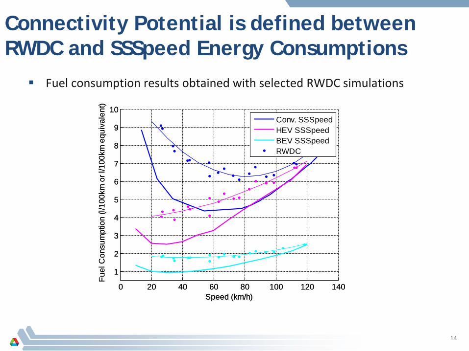
Connectivity Potential is defined between RWDC and SSSpeed Energy Consumptions

Fuel consumption results obtained with selected RWDC simulations

14

0 20 40 60 80 100 120 140

1

2

3

4

5

6

7

8

9

10

Speed (km/h)

Fuel

Con

sum

ptio

n (l/

100k

m o

r l/1

00km

equ

ival

ent)

Conv. SSSpeedHEV SSSpeedBEV SSSpeed

0 20 40 60 80 100 120 140

1

2

3

4

5

6

7

8

9

10

Speed (km/h)

Fuel

Con

sum

ptio

n (l/

100k

m o

r l/1

00km

equ

ival

ent)

Conv. SSSpeedHEV SSSpeedBEV SSSpeedRWDC

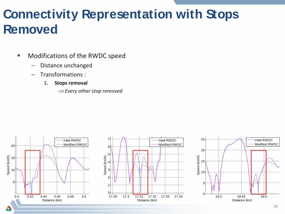
Connectivity Representation with Stops Removed

Modifications of the RWDC speed– Distance unchanged– Transformations :

1. Stops removal⇒ Every other stop removed

15

18.5 18.55 18.60

5

10

15

20

25

Distance (km)S

peed

(km

/h)

Intial RWDCModified RWDC

17.29 17.3 17.31 17.32 17.33 17.340

1

2

3

4

5

6

7

Distance (km)

Spe

ed (k

m/h

)

Intial RWDCModified RWDC

3.4 3.42 3.44 3.46 3.48 3.5

5

10

15

20

Distance (km)

Spe

ed (k

m/h

)

Intial RWDCModified RWDC

Connectivity Representation with Speed Smoothing

Modifications of the RWDC speed– Distance unchanged– Transformations :

1. Stops removal⇒ Every other stop removed

2. Traffic Smoothing⇒ 5s moving average

16

17.2 17.3 17.4 17.5 17.6 17.70

5

10

15

20

25

30

35

Distance (km)

Spe

ed (k

m/h

)

Intial RWDCModified RWDC

8 10 12 14 16 18

95

100

105

110

115

Distance (km)

Spe

ed (k

m/h

)

Intial RWDCModified RWDC

5 6 7 8 9116

118

120

122

124

Distance (km)S

peed

(km

/h)

Intial RWDCModified RWDC

Connectivity Representation with Acceleration Saturation

Modifications of the RWDC speed– Distance unchanged– Transformations:

1. Stops removal⇒ Every other stop removed

2. Traffic Smoothing⇒ 5s moving average

3. Acceleration saturation⇒ by -1.5 and 1.5 m/s2

17

Connectivity Representation with Speed Transformation

Modifications of the RWDC speed– Distance unchanged– Transformations:

1. Stops removal⇒ Every other stop removed

2. Traffic Smoothing⇒ 5s moving average

3. Acceleration saturation⇒ by -1.5 and 1.5 m/s2

4. Speed point by point transformation

18

0 10 20 30 40 500

10

20

30

40

50

Original Speed (km/h)

Tran

sfor

med

Spe

ed (k

m/h

)

28.2 28.4 28.6 28.80

5

10

15

20

25

30

Distance (km)

Spe

ed (k

m/h

)

Intial RWDCModified RWDC

29.5 30 30.5 31 31.50

10

20

30

40

50

60

70

80

Distance (km)

Spe

ed (k

m/h

)

Intial RWDCModified RWDC

16.6 16.7 16.8 16.9

5

10

15

20

25

30

35

40

Distance (km)S

peed

(km

/h)

Intial RWDCModified RWDC

Two Sets of CAV RWDC Defined Modifications of the RWDC speed

– Distance unchanged– Transformations:

1. Stops removal2. Traffic Smoothing3. Acceleration saturation4. Speed point by point transformation

2 CAVs RWDC scenarios:– CAVs RWDC 1 ⇒ Assumptions {1,2,3}

• No speed point by point transformation• 10% PKE decrease• Same averaged speed

– CAVs RWDC 2 ⇒ Assumptions {1,2,3,4} • 12% PKE decrease• Average speed increased at low speed

19

Connectivity Decreases Fuel Consumption Especially at Low Vehicle Speed

Fuel consumption results obtained with selected CAV RWDC simulations

20

0 20 40 60 80 100 120 140

1

2

3

4

5

6

7

8

9

10

Speed (km/h)

Fuel

Con

sum

ptio

n (l/

100k

m o

r l/1

00km

equ

ival

ent)

Conv. SSSpeedHEV SSSpeedBEV SSSpeed

0 20 40 60 80 100 120 140

1

2

3

4

5

6

7

8

9

10

Speed (km/h)

Fuel

Con

sum

ptio

n (l/

100k

m o

r l/1

00km

equ

ival

ent)

Conv. SSSpeedHEV SSSpeedBEV SSSpeedRWDC

0 20 40 60 80 100 120 140

1

2

3

4

5

6

7

8

9

10

Speed (km/h)

Fuel

Con

sum

ptio

n (l/

100k

m o

r l/1

00km

equ

ival

ent)

Conv. SSSpeedHEV SSSpeedBEV SSSpeedRWDC modif. 1

0 20 40 60 80 100 120 140

1

2

3

4

5

6

7

8

9

10

Speed (km/h)

Fuel

Con

sum

ptio

n (l/

100k

m o

r l/1

00km

equ

ival

ent)

Conv. SSSpeedHEV SSSpeedBEV SSSpeedRWDC modif. 2

35 to 50 % Potential Fuel Savings at Low Vehicle Speed

Potential fuel consumption decrease results obtained with selected CAV RWDC simulations

BEVs have biggest potential at low speed

21

20 40 60 80 100 1200

5

10

15

20

25

30

35

40

45

50

Speed (km/h)

Pot

entia

l fue

l Con

sum

ptio

n re

duct

ion

(%)

Fuel Cons. at RWDC speed as reference

Conv.HEV splitBEV

20 40 60 80 100 1200

5

10

15

20

25

30

35

40

45

50

Speed (km/h)

Pot

entia

l fue

l Con

sum

ptio

n re

duct

ion

(%)

Fuel Cons. at RWDC speed as reference

Conv.HEV splitBEV

20 40 60 80 100 1200

5

10

15

20

25

30

35

40

45

50

Speed (km/h)

Pot

entia

l fue

l Con

sum

ptio

n re

duct

ion

(%)

Fuel Cons. at RWDC speed as reference

Conv.HEV splitBEV

Steady-SpeedRWDC CAV1

RWDC CAV2

Virtual Proving Grounds to Quickly Evaluate the Impact of V2V, V2I… on the Energy

VEH1

VEH N

VEH2

Co-simulation of High Fidelity Vehicle Models

Environment Model (1)

Virtual Proving Ground

Sensors/V2X Models

Use cases examples:- Eco-Approach &

Departure at Signalized Intersections

- Eco-Traffic Signal Timing

- Eco-Traffic Signal Priority

- Connected Eco-Driving- Route based control- Impact on traffic flow…

Closed loop control critical for energy and speed optimization22

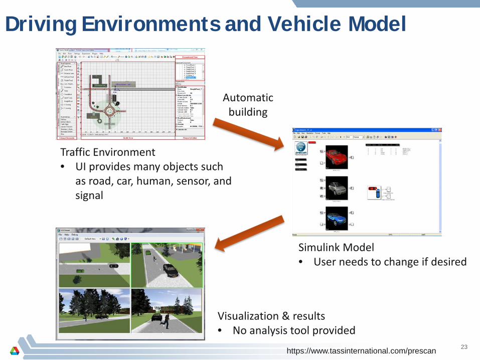
Driving Environments and Vehicle Model

Simulink Model• User needs to change if desired

Traffic Environment• UI provides many objects such

as road, car, human, sensor, and signal

Visualization & results• No analysis tool provided

Automatic building

23https://www.tassinternational.com/prescan

Autonomie Vehicle Models in PreScan

Simulink Model• User needs to change if

desiredElectric Vehicle

HEV

Conventional

High fidelity vehicle models from Autonomie can replace PreScan vehicle model placeholders within Simulink

24

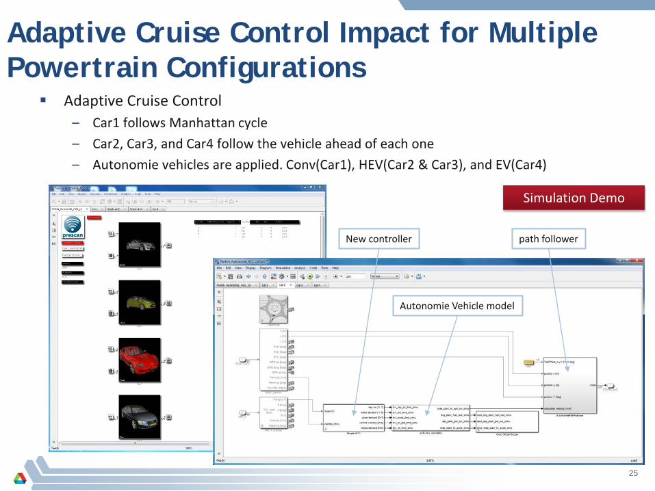
Adaptive Cruise Control Impact for Multiple Powertrain Configurations

Adaptive Cruise Control– Car1 follows Manhattan cycle– Car2, Car3, and Car4 follow the vehicle ahead of each one– Autonomie vehicles are applied. Conv(Car1), HEV(Car2 & Car3), and EV(Car4)

path followerNew controller

Autonomie Vehicle model

Simulation Demo

25

[main_info_bus]

[whl]

whl

[main_info_bus]

[tc]

tc

[main_info_bus]

[str]

str

[str_3]

gotostr_3

[gen_3]

gotogen_3

[cpl_3]

gotocpl_3

-T-

gotoaccelec_3

[main_info_bus]

[gen]

gen

[main_info_bus]

[gb]

gb

[str_3][gen_3]

[cpl_3]-T-

[main_info_bus]

[fd]

fd

[main_info_bus]

[ess]

ess

[main_info_bus]

[eng]

eng

[main_info_bus]

[cpl]

cpl

[main_info_bus]

[chas]

chas

[main_info_bus]

[accmech]

accmech

[main_info_bus]

[accelec]

accelec

26

Transportation Simulation Powertrain Simulation

Fleet Definition

Energy consumption of the transportation network

At the Fleet Level, Large Transportation System Models are Required to Evaluate CAVs ImpactUse cases examples:- Eco-Lanes (dedicated freeway, variable speed limits, ECACC…)- Wireless charging (bus lanes)- Low Emissions Zones- Platooning- Smoother braking- Mixed vehicle fleet (i.e. HEVs, BEVs + few CAVs)- Increased VMT due to travel behavior changes- Charging station location…

Integrated Transportation Model ( )

NETWORK MODEL Physical laws that govern dynamics of

traffic flow Newell’s model Managed Lanes Controlled intersections (traffic signals) Traveler information systems Traffic management Multimodal travel (Integrated

corridor management)27

POLARIS is an agent-based transportation system model

Decision making is decentralized. Each traveler has its own goals and behaviors. All aspects of activity and travel are represented in a single model

Travelers are autonomous and can adopt to current conditions (congestion, mode availability, information available)

Not restricted to a limited number of market segments (user groups)

The agent based framework is flexible and can accommodate other types of agents (buildings, authorities, smart infrastructure)

Integrated Transportation System Model ( )

28

Individual Activity Travel Patterns Allow Accurate Drive Cycle Evaluation

1:55 PMReturn to Work

6:30PMShop

2:45 PMOff Train

9:15 AMDrop off

9:15 AMDay Care

3:50 PMPick up

7:15 PMReturn

9:00 AMLeave Home

8:00 AMLeave Home

8:15 AMOn Train

9:00AMLeave Home

4:10PMReturn 4:10 PM

Return

Drive Trip

Passenger Trip

Train Trip

Activity Locations

In Chicago over 46% of time away from home is not at a work or school location

1:15 PMLunch

10:00 AMArrive at Work

3:00 PMRecreation

29

Evaluating the Energy Impact of an Automation Scenario

30

Powertrain Technologies • Each vehicle class has a conventional ICE version

(CV) and a hybrid (HEV) version • Each vehicle template has a unique combination of

components and average mass

3 Scenarios: • UM: Unmanaged • ML: Managed lane for heavy-duty trucks • ML+ACC: Managed lane for trucks, and all trucks have

adaptive cruise control (ACC)

18 km Stretch of Highway in Chicago 25 on- and off- ramps

Evaluating the Energy Impact of an Automation Scenario

• With managed lanes, the savings are lower, and non-existent when ACC is used. This is because braking, and its recuperation, is virtually eliminated.

• Overall fuel savings for trucks:–- managed lanes (ML): 25%–- managed lanes + ACC: 40%

31

Fuel Consumption Distribution (all trucks, FS1)

Average Truck Fuel Consumption

• Class 8 hybridization (“mild” with ISG) saves approx. 15% in the unmanaged case; for class 6 (“full HEV”), savings are approx. 20%.

• With managed lanes, the savings are lower, and non-existent when ACC is used (No regen braking)

Conclusion

• A lot of good work has been performed, but since the focus has been forconventional vehicles at the individual level, additional in-depth analysisneeds to be performed to assess the impact on energy.

• At the vehicle level using CAV-like RWDC, we showed that,– Connectivity decreases fuel consumption especially at low speed– 35 to 50 % connectivity potential fuel savings at low speed

• BEVs have biggest potential at low speed

– Connectivity doesn’t modify the hybridization potential• System level analysis has to be performed including uncertainty using new

set of tools.• The potential increase in travel demand could reverse the recent

significant gains.• Advanced vehicle technologies such as electrified vehicles could minimize

the impact of the demand effect through fuel energy diversification.• CAVs could lead to an increase in advanced vehicles market penetration

32