impact of corrosion inhibitors on lead release and biofilm ... · impact of corrosion inhibitors on...

Impact of Corrosion Inhibitors on Lead Release and Biofilm

Development in Simulated Partial Lead Service Lines

by

Aki Kogo

A thesis submitted in conformity with the requirements

for the degree of Master of Applied Science

Civil Engineering

University of Toronto

© Copyright by Aki Kogo 2016

ii

Impact of Corrosion Inhibitors on Lead Release and Biofilm

Development in Simulated Partial Lead Service Lines

Aki Kogo

Master of Applied Science, 2016

Graduate Department of Civil Engineering

University of Toronto

ABSTRACT

Partial lead service line replacements intended to decrease lead in drinking water but found to

potentially increase lead release by galvanic corrosion. This study investigated the effects of

corrosion inhibitors on lead release in simulate partial lead service lines. The performance of

orthophosphate, zinc orthophosphate, and sodium silicate were compared under different water

quality conditions (CSMR, conductivity, chlorination). Both orthophosphate and zinc

orthophosphate immediately decreased lead release in all conditions, while sodium silicate

seemed to slowly decrease lead release over time.

Biofilm is a potential reservoir of lead in distribution systems, and the detachment of biofilm

containing lead particles can cause health risk in drinking water. The effect of corrosion control

on biofilm development was also examined under stagnant and flow-through conditions.

Chlorination significantly decreased biofilm and was effective both under stagnant and flow-

through conditions. The densities of ATP and lead in biofilm were typically consistent.

iii

ACKOWLEDGEMENTS

This project was funded by Canadian Water Network (CWN), and I gratefully thank CWN for

the financial support.

I would like to thank my supervisor Prof. Robert C. Andrews, Sarah Jane Payne, and Jim Wang

for walking through this project with me as a team. Your guidance, support, and encouragement

were indispensable to accomplish this project. Also, I appreciate Dave Scott and all the staff at

the R. C. Harris Water Treatment Plant for providing source water for this project. I would like

to thank everyone in Drinking Water Research Group. It was a great time for me to work with

you all. Finally, I thank my family and friends for your continued support and encouragement.

iv

TABLE OF CONTENTS ABSTRACT .................................................................................................................................... ii

ACKOWLEDGEMENTS .............................................................................................................. iii

TABLE OF CONTENTS ............................................................................................................... iv

LIST OF TABLES ........................................................................................................................ vii

LIST OF FIGURES ....................................................................................................................... ix

NOMENTCLATURE .................................................................................................................... xi

1 Introduction .................................................................................................................................1

1.1 Background ..........................................................................................................................1

1.2 Objective ..............................................................................................................................3

1.3 Description of Chapters .......................................................................................................3

2 Literature Review ........................................................................................................................4

2.1 Lead Release From Lead Service Lines ...............................................................................4

2.1.1 Galvanic Corrosion ..................................................................................................4

2.1.2 Precipitation and Dissolution of Pipe Scales ...........................................................5

2.2 Water Chemistry Affecting Lead Release ...........................................................................6

2.2.1 CSMR ......................................................................................................................6

2.2.2 Alkalinity and pH .....................................................................................................8

2.2.3 Corrosion Inhibitors .................................................................................................9

2.2.4 Disinfectant: Chlorine in Comparison to Chloramine ...........................................11

2.3 Bacterial Regrowth and Biofilm Formation in Distribution Systems ................................12

3 Materials and Methods ..............................................................................................................13

3.1 Experimental Setup ............................................................................................................13

3.1.1 Pipe Loops for Partial Lead Service Line Replacement Study ..............................13

3.1.2 Pipe Loops for Biofilm Study ................................................................................14

3.1.3 Lead Release During Stagnation Periods ...............................................................15

3.1.4 Mass Balance .........................................................................................................17

3.1.5 Experimental Timeline...........................................................................................17

3.1.6 pH Control in the Reservoirs .................................................................................18

3.1.7 Preparation of A Free Chlorine Working Solution ................................................19

3.2 Analytical Methods ............................................................................................................19

3.2.1 Total and Dissolved Metals (Lead and Copper) ....................................................19

v

3.2.2 Galvanic Current ....................................................................................................20

3.2.3 Alkalinity ...............................................................................................................20

3.2.4 pH ...........................................................................................................................21

3.2.5 Turbidity ................................................................................................................21

3.2.6 Total Organic Carbon ............................................................................................21

3.2.7 Chloride, Sulfate, Phosphate, Nitrate, and Nitrite .................................................22

3.2.8 Silica ......................................................................................................................23

3.2.9 Free Chlorine .........................................................................................................23

3.2.10 ATP ........................................................................................................................23

3.3 Statistical Analysis .............................................................................................................24

4 Comparison of Three Corrosion Inhibitors in Simulated Partial Lead service Line

Replacements ............................................................................................................................25

4.1 Abstract ..............................................................................................................................25

4.2 Introduction ........................................................................................................................25

4.3 Materials and Methods .......................................................................................................29

4.3.1 Partial Lead Service Line Experimental Setup ......................................................29

4.3.2 Experimental Plan ..................................................................................................32

4.3.3 Experimental Design ..............................................................................................34

4.3.4 Sample Analysis.....................................................................................................34

4.3.5 Statistical Analysis .................................................................................................35

4.4 Results and Discussion ......................................................................................................36

4.4.1 Effects of corrosion inhibitors for different stagnation periods .............................36

4.4.2 Effects of CMSR and conductivity ........................................................................40

4.4.3 Effects of Galvanic corrosion ................................................................................42

4.4.4 Comparison of dissolved and particulate lead release ...........................................46

4.4.5 Copper release during acclimation and treatment ..................................................47

4.5 Conclusions ........................................................................................................................51

5 Impact of Corrosion Control on Biofilm Development in Simulated Partial Lead Service

Line Replacements ....................................................................................................................52

5.1 Abstract ..............................................................................................................................52

5.2 Introduction ........................................................................................................................52

5.3 Materials and Methods .......................................................................................................54

vi

5.3.1 Partial lead service line setup .................................................................................54

5.3.2 Experimental plan ..................................................................................................56

5.3.3 Sample Analysis.....................................................................................................56

5.3.4 Estimation of lead released through galvanic current ............................................58

5.3.5 Statistical Analysis .................................................................................................58

5.4 Results and Discussion ......................................................................................................58

5.4.1 Effects of corrosion inhibitors on biofilm growth under stagnant and flow-

through conditions .................................................................................................58

5.4.2 Estimation of capacity of biofilm for storing lead .................................................67

5.5 Conclusion .........................................................................................................................69

6 References .................................................................................................................................70

7 Appendices ................................................................................................................................81

7.1 Sample Quality Assurance/Quality Control Charts ...........................................................81

7.2 Raw Data ............................................................................................................................85

7.3 Preliminary Results ..........................................................................................................115

7.3.1 Tank Acidification ...............................................................................................115

7.3.2 Chlorine Demand Test .........................................................................................119

vii

LIST OF TABLES

Table 3-1: Pipe Loop Test Section Composition .......................................................................... 14

Table 3-2: Typical Daily Flow Pattern used in Experiments from Friday Evening to Tuesday

evening .......................................................................................................................................... 15

Table 3-3: Timeline for Experiments ............................................................................................ 18

Table 3-4: Reagents for Alkalinity Analysis ................................................................................ 21

Table 3-5: Reagents for TOC and DOC Analysis ........................................................................ 22

Table 3-6: Instrumental Conditions for TOC and DOC Analysis ................................................ 22

Table 4-1: Experimental conditions for both acclimation and treatment phases (OP, ZOP, sodium

silicate) .......................................................................................................................................... 31

Table 4-2: Characteristics of raw Lake Ontario water used for the experiments ......................... 32

Table 4-3: Recirculation event and sample collection for a weekly cycle ................................... 33

Table 4-4: Event in a weekly cycle ............................................................................................... 33

Table 4-5: Comparison of dissolved and total lead release (± standard deviation) ...................... 39

Table 5-1: Experimental conditions for both acclimation and corrosion inhibitor trials (OP, ZOP,

and sodium silicate) ...................................................................................................................... 55

Table 5-2: Raw water quality ........................................................................................................ 56

Table 5-3: Log reduction in ATP in stagnant and flow-through biofilm by chlorination ............ 60

Table 5-4: Particulate lead fraction in biofilm and bulk water (at the end of a weekly cycle) ..... 66

Table 5-5: Estimation of lead storing capacity of biofilm and removal from theoretical weekly

mass release .................................................................................................................................. 68

Table 7-1: Total and dissolved lead release for 30-min stagnation periods (part 1) ..................... 85

viii

Table 7-2: Total and dissolved lead release for 6-h stagnation periods (part 1) ........................... 88

Table 7-3: Total and dissolved lead release for 65-h stagnation periods (part 1) ......................... 91

Table 7-4: Lead concentrations in samples of pre-acidification bulk water (90 L) and acidified

bottom 20 L of reservoir water (part 1) ........................................................................................ 93

Table 7-5: Weekly mass release calculated based on samples collected (part 1) ......................... 96

Table 7-6: Total and dissolved copper release for 30-min stagnation periods (part 1) ................ 98

Table 7-7: Total and dissolved copper release for 6-h stagnation periods (part 1) ..................... 101

Table 7-8: Total and dissolved copper release for 65-h stagnation periods (part 1) ................... 104

Table 7-9: Copper concentrations in samples of pre-acidification bulk water (90 L) and acidified

bottom 20 L of reservoir water (part 1) ...................................................................................... 106

Table 7-10: Total and dissolved lead accumulation in biofilm under stagnant and flow-through

conditions .................................................................................................................................... 109

Table 7-11: Total and dissolved copper accumulation in biofilm under stagnant and flow-through

conditions .................................................................................................................................... 110

Table 7-12: ATP accumulation under stagnant (Stag) and flow-through (Flow) conditions ..... 111

Table 7-13: Average galvanic current (± standard deviation) .................................................... 112

Table 7-14: Water quality parameters of reservoir water (part 1) .............................................. 113

ix

LIST OF FIGURES

Figure 3-1: Typical pipe loop system ........................................................................................... 14

Figure 3-2: Weekly Cycle and Sampling Times ........................................................................... 16

Figure 4-1: Comparison of average dissolved (blue) and particulate (black) lead release for each

corrosion inhibitors (a. 30 min, b. 6 h, c. 65 h). ............................................................................ 38

Figure 4-2: Galvanic current in Cu-Pb systems during three treatment phases. ........................... 41

Figure 4-3: Predicted vs. observed total lead release for 6-h stagnation period under conditions of

a) low CSMR, b) high CSMR-low conductivity, c) high CSMR-high conductivity, and d) high

CSMR-high conductivity-chlorine................................................................................................ 44

Figure 4-4: Average weekly lead release. ..................................................................................... 45

Figure 4-5: Comparison of average dissolved (blue) and particulate (black) copper release for

each corrosion inhibitors (a. 30 min, b. 6 h, c. 65 h). ................................................................... 50

Figure 5-1: ATP accumulation under a) stagnant and b) flow-through conditions. n=4, 2, 2, and 8

for low CSMR, high CSMR-low conductivity, high CSMR-high conductivity, and high CSMR-

high conductivity-chlorine phases. ............................................................................................... 61

Figure 5-2: Total lead and ATP accumulation under a) stagnant and b) flow-through conditions

(linear regression). ........................................................................................................................ 62

Figure 5-3: Lead accumulating in biofilm under a) stagnant and b) flow-through conditions with

and without chlorination. n=2 and 8 for high CSMR-high conductivity and high CSMR-high

conductivity-chlorine phases. ....................................................................................................... 63

Figure 5-4: Copper accumulating in biofilm under a) stagnant and b) flow-through conditions

with and without chlorination. ...................................................................................................... 64


with and without chlorination. n=2 and 8 for high CSMR-high conductivity and high CSMR-

high conductivity-chlorine phases. ............................................................................................... 65

x

Figure 7-1: QC chart – lead (Check standards = 100 µg/L) ......................................................... 82

Figure 7-2: QC chart – copper (Check standards = 100 µg/L) ..................................................... 82

Figure 7-3: QC chart – TOC (Check standards = 2.5 mg/L) ........................................................ 83

Figure 7-4: QC chart – phosphate (Check standards = 2.0 mg/L) ................................................ 83

Figure 7-5 : QC chart – chloride (Check standards = 25 mg/L) ................................................... 84

Figure 7-6: QC chart – sulfate (Check standards = 30 mg/L)....................................................... 84

Figure 7-7: Daily galvanic current .............................................................................................. 112

Figure 7-8: Treatments to Determine Lead Recovery from Reservoirs ..................................... 116

Figure 7-9: Lead Concentrations During 50-h Acidification ...................................................... 118

Figure 7-10: Free chlorine concentrations in 1 L of waters from the six reservoirs (second

time)Control of the free chlorine and monochloramine residual in the reservoirs .................... 120

xi

NOMENTCLATURE

≈ approximate

< Less than

> Greater than

≤ Less than or euqual to

- To

± Plas/minus

α Confidence level

μg/L Microgram(s) per liter

μL Microlitrer(s)

μm Micrometer(s)

Ω Ohm(s)

% Percent

ATP Adenosine triphosphate

APHA American Public Health Association

AWWA American Water Works Association

BLL Blood lead level

cm Centimeter(s)

Cl- Chloride ion

CSMR Chloride to sulfate mass ratio

Cl2 Chlorine

CFU/cm2 Colony forming unit per centimeter squared

CFU/L Colony forming unit per liter

CI Confidence interval

Cu Copper

° C Degrees Celsius

d Diameter

DBP Disinfection by-product

DIC Dissolved inorganic carbon

e Electron

EPA Environmental protection agancy

xii

N Equivalent concentration (eq/L)

EPS Exopolysaccharide

g Gram(s)

g/L Gram(s) per liter

HPC Heterotrophic plate count(s)

h Hour(s)

h/day Hour(s) per day

ICP-OES Inductively coupled plasma optical emission spectrometry

Fe Iron

Pb Lead

Pb(IV) Lead (4+), Pb4+

PbO2 Lead dioxide

LSL Lead service line

Pb(II) Lead(2+), Pb2+

LPM Liter per minute

L Liter(s)

L/day Liter(s) per day

L/min Liter(s) per minute

pH -log (hydrogen ion concentration)

Mn Manganese

MPI Metabolic potential index

mg/L Milligram(s) per liter

mL Milliliter(s)

mm Millimeter(s)

mS/cm Millisiemens per centimeter

min Minute(s)

M Molar concentration (mol/liter)

NH2Cl Monochloramine

ng/cm2 Nanogram per centimeter squared

nm Nanometer(s)

NTU Nephelometric turbidity unit(s)

N/m2 Newton per meter squared

xiii

ON Ontario

OP Orthophosphate

ORP Oxidation reduction potential

PLSLR Partial lead service line replacement

Pa Pascal

R2 Pearson’s correlation coefficient

P Phosphorus

PVC polyvinyl chloride

QA/QC Quality assurance quality control

RLU Relative light units

SO4- Sulfate ion

TDC Total direct count

TOC Total organic carbon

U.S. United States

USA United States of America

v/v Volume per volume

ZOP Zinc orthophosphate

1

1 Introduction

1.1 Background

The events of increased lead leaching to drinking water occurred in Flint, Michigan in 2014-

2016 (Kennedy et al., 2016) and Washington, DC in 2001-2004 (Edwards and Dudi, 2004) raised

public concern to lead contamination in drinking water. Those cases happened when the utilities

changed the chemical characteristics of water by changing the water source from Lake Huron to

Flint River, which was more corrosive (Kennedy et al., 2016), or switched the disinfectant from

chlorine to chloramine to manage the formation of disinfectant by-products (Edwards and Dudi,

2004).

The complexity and difficulty for lead control in drinking water is also attributed to distribution

systems. Drinking water is a source of human exposure to lead along with air, house dust, and

food (Health Canada, 2013). It was estimated that lead in drinking water accounts for

approximately 20% of lead entering a human body (U.S. EPA, 2002). Following the inhibition of

lead pipe installation in drinking water distribution systems in 1986 in the U.S. (U.S. EPA, 2015)

and in 1975 for lead pipes and 1986 for solder in Canada (Health Canada, 2007), the strategy of

PLSLR was employed to decrease lead in drinking water by removing lead pipes in distribution

systems. However, it was found PLSLR may not significantly decrease BLLs of children when

compared to full LSLs (Brown et al., 2011) and can increase lead release due to galvanic

corrosion between lead and copper (Cartier et al., 2013; Wang et al., 2013) in addition to

temporary but serious lead release by physical disturbance at replacement (Zietz et al., 2001).

Galvanic corrosion can increase lead release while protecting the copper side by cathodic

protection and can elevate lead concentrations in water for weeks (Wang et al., 2013; Edwards

and Triantafyllidou, 2007) to months (Triantafyllidou and Edwards, 2011).

CSMR have effects on lead release by changing the composition of lead products. Higher CSMR

can be resulted from the source water and the use of chloride-based coagulants during treatment

processes and tends to increase lead release. The critical CSMR that can increase lead corrosion

was estimated to be 0.5-0.77 (Gregory, 1985; Dodrill and Edwards, 1995; Nguyen et al., 2011b).

In addition, it was considered higher conductivity affects galvanic corrosion. Willison and Boyer

2

(2012) observed the water with higher concentrations of chloride and sulfate had higher lead

leaching than lower concentrations with the consistent CSMR.

It is also necessary to search for alternatives to conventional corrosion inhibitors in cases of

waters in which phosphate being ineffective or unfeasible cost. Phosphate is a common corrosion

inhibitor for lead control, and McNeill and Edwards (2002) reported 56% of utilities used

phosphate-based inhibitors for lead control in 2001. However, the price of phosphate rock is

volatile and increased by 800% in 2007-2008 (McGill, 2012). ZOP, in comparison to OP, was

reported to increase particulate lead release (McNeill and Edwards, 2004). It is concerned the use

of phosphate-based inhibitors can increase microbial activity in drinking water (McNeill and

Edwards, 2002). Biofilm can be a sink for particles released from pipe materials, but the capacity

of biofilm storing lead is not well-documented. Ginege et al. (2011) reported the ability of

biofilm to remove iron and manganese both under unchlorinated and chlorinated condition.

Detachment of biofilm can cause release of trapped iron and manganese (Ginege et al., 2011),

which can be applicable to lead as well. Deshommes and Prévost (2012) reported ingestion of

lead particles in tap water can contribute to the exposure of children to lead. Sodium silicate can

be a potential alternative to phosphate-based inhibitors (Dart and Foley, 1970) and has been used

for iron control in drinking water (Robinson et al., 1992). Past studies showed sodium silicate

effectively decreased lead release (Schock et al., 2005; Lintereur et al., 2010; Sastri et al., 2006).

It was reported that the effect of sodium silicate may take time to appear because of slow

formation of silicate film (Thompson et al., 1997; Schock et al., 2005).

The events of lead leaching in drinking water reminded that the situation regarding drinking

water is complicated. This study provided a realistic simulation of PLSLRs to investigate

corrosion inhibitors under various water qualities.

3

1.2 Objective

This thesis investigated the following objectives:

1. Compare the performance of three corrosion inhibitors (orthophosphate, zinc

orthophosphate, and sodium silicate) to mitigate lead release in PLSLR under two levels

of CSMR and conductivity in the absence and presence of free chlorine.

2. Examine the impact of free chlorine on biofilm and bulk water microbiology in the

presence of three corrosion inhibitors in partial LSLs.

1.3 Description of Chapters

Chapter 2 provides a literature review of past studies regarding lead control strategies and

factors affecting lead release.

Chapter 3 contains the materials and methods used to conduct the experiments for this

study.

Chapter 4 examines the effects of corrosion inhibitors on lead release in simulated partial

lead service line replacement under different water quality conditions.

Chapter 5 evaluates the effects of corrosion inhibitors on biofilm development under non-

chlorinated and chlorinated conditions.

Chapter 6 provides the list of references used in this study.

Chapter 7 provides the appendices, including the results of preliminary study, the QA/QC

chart, and the raw data.

4

2 Literature Review

2.1 Lead Release From Lead Service Lines

Lead in drinking water can be attributed from two main mechanisms: galvanic corrosion and

dissolution of leaded pipe scales.

2.1.1 Galvanic Corrosion

Galvanic corrosion occurs when dissimilar metals with different electrochemical potentials

become connected and are in contact with an electrolyte. In a galvanic coupling, the metal with

higher electrochemical potential corrodes. In a system with partial lead service line replacement

(PLSLR) in which a lead pipe is galvanically connected to a copper pipe, lead acts as an anode

and copper as a cathode. Water flowing through the pipes acts as the electrolyte and provides a

pathway for ions to migrate. The following half reactions and the net reaction occur when lead

enters solution (Wang et al., 2012; Sastri et al., 2006).

Pb (s) = Pb2+ + 2e− 2-1

O2(aq) + 4H+ + 4e− = 2H2O 2-2

2Pb (s) + O2(aq) + 4H+ = 2Pb2+ + 2H2O 2-3

Occurrence of galvanic corrosion can be observed by measuring current between lead and copper

pipes. Galvanic currents have been shown to have a positive linear correlation with lead with R2

values of 0.93 and 0.77 reported by Nguyen et al. (2010) and Hu et al. (2012), respectively.

Galvanically connected systems have shown an increase in lead concentration by a factor of 5.5

(Cartier et al., 2013). Wang et al. (2013) also observed an eight-fold increase in total lead

concentration after a 6 hour stagnation following installation of an external wire connecting a

lead pipe to a copper pipe. Following removal of the external wire, lead concentration

immediately decreased to the same level as that without galvanic corrosion (Wang et al., 2013).

Galvanic corrosion has also been observed in lead bearing brass to copper connections. In a

study conducted by Cartier et al. (2012b), lead concentration increased by a factor of 2.4 in a

faucet composed of red brass which was connected to a copper nipple.

5

Even though PLSLR without galvanic corrosion can increase lead release in distribution systems,

galvanic corrosion can exacerbate lead release in the systems. Elevated lead concentrations were

presumably attributed from mechanical disturbance due to PLSLR or pipe repair in

approximately 50% of households examined in Lower Saxony, Germany (Zietz et al., 2001).

Lead release due to mechanical disturbance increases lead concentrations for a short period of

time. High lead concentrations were observed in waters for the first 15 min following non-

galvanic connection of pipes, and the concentration declined below 10 µg/L afterward (Boyd et

al., 2004). However, PLSLR with galvanic connection can further increase lead concentrations

and have a prolonged impact, as galvanic current has been reported to persist over 6 weeks

(Wang et al., 2013), 11 weeks (Edwards and Triantafyllidou, 2007), and several months

(Triantafyllidou and Edwards, 2011).

The extent of galvanic corrosion also varies depending on other factors, including stagnation

period and flow rate. Wang et al. (2012) reported that, when compared to systems without

galvanic corrosion, 6-h and 65-h stagnations increased total lead leaching due to galvanic

corrosion by 4-6 and 15-30 times, respectively. Similarly, lead release from galvanic systems of

lead solder and copper pipe rigs increased in waters regardless of disinfectant type (free chlorine

and chloramines) by increasing stagnation time from 30 min to 24 h (Woszczyski et al., 2013).

Lytle and Schock (2000) observed exponential increases in lead concentrations over a 90 h

stagnation period, with 50-70% of lead leaching during the first ten hours. The impact of flow

rate was investigated in Cartier et al. (2013), and particulate lead release significantly (p < 0.05)

increased by a factor of 12 on an average regardless of treatment when the flow rate was raised;

particulate lead release from pure lead pipes, for example, increased from 21±16 to 284±314

µg/L as flow rate was increased from 5 to 15 LPM. In contrast, dissolved lead concentration

showed a limited impact of flow rate change (Cartier et al., 2013).

2.1.2 Precipitation and Dissolution of Pipe Scales

Precipitation and dissolution of leaded pipe scales are major factors affecting lead concentrations

in drinking water, and are controlled by water chemistry and presence of corrosion inhibitors.

Studies have shown that leaded pipe scales are composed of various compounds, including Pb(II)

carbonates, Pb(II) oxides, and Pb(IV) oxides (Schock et al., 2008). A Pb(II) carbonate

6

hydrocerussite (Pb3(CO3)2(OH)2) is a widely observed component of leaded pipe scales (Kim

and Herrera, 2010; Hozalski et al., 2005; Noel et al., 2014). Released lead can precipitate onto

the surface of pipes, forming passivating scales (Lintereur et al., 2010). Under conditions of high

redox potential, PbO2 precipitates along with dominant or coexisting Pb (II) mineral forms

hydrocerussite and cerussite (Lytle and Schock, 2005).

Lead release from scale dissolution was strongly affected by pH and dissolved inorganic carbon

(DIC), and the steady-state concentrations of hydrocerussite decreased with increasing pH from

6 to 10 when the water had 0 mg/L DIC (Noel et al., 2014). Similarly, decreasing pH from 10 to

8.5 resulted in increased lead due to the dissolution of hydrocerussite and lead oxides (Xie and

Giammer, 2011). Increasing DIC from 0 to 10 mg/L decreased hydrocerussite dissolution,

however increasing DIC to 50 mg/L did not reduce the dissolution further (Noel et al., 2014).

Conversely, increasing DIC can enhance dissolution of corrosion products by reducing Pb(IV) to

Pb(II) and by forming soluble Pb(II) (Xie et al., 2010). Also, physical conditions of water

including flow rates and stagnation periods, can increase the rates of lead scale dissolution. It

was demonstrated that, when compared to stagnant water, flowing water had considerably

accelerated dissolved lead release rates, even though higher lead release would occur during

stagnation periods due to longer contact time between water and pipe during stagnation than

flowing periods (Xie and Giammer, 2011).

2.2 Water Chemistry Affecting Lead Release

Various water parameters can have strong impacts on lead release from distribution systems.

2.2.1 CSMR

Chloride-to-sulfate mass ratio (CSMR) shows the relative mass of chloride to sulfate, and CSMR

can be calculated using the equation shown below (Edwards and Triantafyllidou, 2007).

𝐶𝑆𝑀𝑅 =

[𝐶𝑙−]

[𝑆𝑂42−]

2-4

7

CSMR of water can be affected by the compositions of specific coagulants used in drinking

water treatment. Application of chloride-based and sulfate-based coagulants during treatment

results in high and low CSMRs, respectively. Studies have shown that waters with high CSMR

can enhance galvanic corrosion. Conductivity tends to increase in high CSMR, which facilitates

galvanic current and consequently galvanic corrosion (Gregory, 1985; Willison and Boyer,

2012). The critical values of CSMR that can enhance lead corrosion to unacceptably high levels

are estimated to be 0.5 (Gregory, 1985), 0.58 (Dodrill and Edwards, 1995), and 0.77 (Nguyen et

al., 2011b). Edwards and Triantafyllidou (2007) treated water with polyalminum chloride and

alum to compare high and low CSMR conditions, and the authors reported that the higher CSMR

(1.42-4.5) waters had 1.5 to 3 times higher lead leaching from solder than the low CSMR (0.5)

waters. Also, significant (95% CI) pH drops were observed in both higher and lower CSMR

galvanic samples, declining from 7.6-7.8 to as low as 3.4 and 4.4 near the solder surface,

respectively (Edwards and Triantafyllidou, 2007). Nguyen et al. (2011c) found increasing CSMR

from 0.1 to 1.0 resulted in an increase in galvanic corrosion from 50:50 lead-tin solders, but

increasing CSMR higher than 1.0 did not have an additional impact in some of the waters which

they investigated. Wang et al. (2013) did not observe an increase in total lead release when

increasing CSMR from 0.7 to 7 and presumed this may be because a high initial CSMR of 0.7

had already enhanced lead corrosion for this system.

Even though CSMR can be used to predict lead corrosion in water, high chloride and sulfate

concentrations can result in enhanced lead release. Willison and Boyer (2012) examined higher

concentrations of chloride and sulfate while the CSMR value was kept constant (0.5). It was

demonstrated that water with higher concentrations of chloride (50 mg/L) and sulfate (100 mg/L)

had significantly (95% CI) higher lead release than waters with lower concentrations (5 mg Cl-/L

and 100 mg SO42-/L) (Willison and Boyer, 2012). Since anions, such as chloride and sulfate, can

be drawn toward the anode surface due to galvanic corrosion, concentrations of anions and

locally high CSMR in the microenvironment around the anode can influence lead corrosion

(Nguyen et al., 2010). In addition, a pH drop from 8.3 to 6.4 was observed within 5 cm of

galvanic junction after 1 h stagnation under both high (16.2) and low (0.2) CSMR conditions,

indicating galvanic corrosion created a corrosive microenvironment at the junction (Hu et al.,

2012).

8

2.2.2 Alkalinity and pH

Alkalinity is used to represent the capacity of a solution to neutralize an acid and has indirect

impacts on lead corrosion. In addition, pH is also an important factor that is often interrelated

with alkalinity. Alkalinity and high pH are considered to be beneficial when considering

corrosion control of lead. When compared to 15 mg/L as CaCO3, water with 45 mg/L as CaCO3

or higher alkalinity resulted in decreased lead release at pH 7.2 (McNeill and Edwards, 2004).

Similarly, assessment of waters without corrosion inhibitors by Dodrill and Edwards (1995)

reported that higher 90th percentile lead concentrations were observed in waters with alkalinity <

30 mg/L as CaCO3 and for pH ranges of < 7.40, 7.40-7.80, and 7.80-8.40, ranging from

approximately 0.024-0.034 mg/L, when compared to most waters with the higher alkalinity (> 30

mg/L). Lead release tended to decrease for alkalinities in the ranges of 30-74, 74-174, and > 174

mg/L as CaCO3, except when water had 30-74 mg/L alkalinity as CaCO3 and pH < 7.40 (Dodrill

and Edwards, 1995). Edwards et al. (1999) showed that increasing alkalinity resulted in

decreases in 90th percentile lead concentrations. The same study estimated an optimum alkalinity

range to be 20-40 mg/L as CaCO3 at pH > 8.5 for lead corrosion control (Edwards et al., 1999).

In contrast, addition of 100 to 150 mg/L alkalinity as CaCO3 resulted in three to five time higher

lead concentrations at pH 7, when compared to controls with 20 mg/L alkalinity as CaCO3; lead

concentrations of approximately 230, 210, and 350 µg/L in the samples with 100, 125, 150 mg/L

alkalinity while approximately 70 µg/L in control (Tam and Elefsinotis, 2009). However, the

effects of alkalinity on lead concentrations became insignificant at pH > 8 (Tam and Elefsinotis,

2009). Also, an increase in pH (7.7-8.4) and alkalinity (80-240 mg/L) resulted in a decrease in

lead concentrations in a 1-year pilot study (Tang et al., 2006). Similarly, raising pH to 8.4 was

effective in a new faucet (30% reduction) with and without connection to copper piping (Cartier

et al. 2012b). Nguyen et al. (2011c) adjusted CSMR in 100 % distribution water (alkalinity 125

mg/L as CaCO3) and a 75:25 desalinated: distribution water blend (61 mg/L as CaCO3) to be 1.1

to examine the effect of alkalinity. The blended water increased lead release from approximately

60 µg/L to 560 µg/L, when compared to the 100% distribution water (Nguyen et al., 2011c).

Low pH prevents formation of passivated scales on the lead anode and thus increases lead

leaching via continuous galvanic corrosion. Although alkalinity can buffer pH and decrease

corrosion, increased conductivity due to alkalinity may outweigh the benefit. Nguyen et al.

9

(2011c) showed that galvanic lead corrosion was promoted when alkalinity was < 10 mg/L

CaCO3, while galvanic corrosion was mitigated by scale formation on the lead anode when

alkalinity was > 10 mg/L as CaCO3.

2.2.3 Corrosion Inhibitors

Corrosion inhibitors may be added to treated water to reduce lead release from distribution pipes.

2.2.3.1 Orthophosphate and Zinc Orthophosphate

Phosphate-based inhibitors are commonly applied to control lead corrosion in drinking water

distribution systems. Use of orthophosphate is becoming increasingly common, growing from

5% (of utilities employing phosphate inhibitors using orthophosphate in 1994) to approximately

20% in 2001 (McNeill and Edwards, 2002). Zinc orthophosphate is another common corrosion

inhibitor, being applied at approximately 30% of the utilities using phosphate inhibitors in 2001

(McNeill and Edwards, 2002). Tam and Elefsinotis (2009) reported that the addition of

orthophosphate (0.8 mg P/L) decreased lead release by 70% for a pH of 7.5 and was also

effective at the higher pH (8.0). Similarly, Cartier et al. (2013) showed the addition of

orthophosphate reduced 64% of lead release (from 72±14 to 26±9 µg/L) for pure lead pipes

within 8 days of application. The effectiveness of orthophosphate has been reported in other

studies as well (Cardew 2009; Cartier et al., 2012b; Edwards and McNeill, 2002).

Orthophosphate tends to be more effective on the soluble lead portion. Addition of

orthophosphate suppressed dissolved lead concentrations to be 21±15 µg/L following a galvanic

connection with copper pipe (Cartier et al., 2012b). Water treated with zinc orthophosphate (0.37

and 1.0 mg/L) resulted in significantly (95% CI) lower lead concentrations following 4 months

and 8 months, when compared to a control (Churchill et al., 2000). When comparing

orthophosphate and zinc orthophosphate, both inhibitors significantly reduced (95% CI) lead

release from brass and solder galvanically connected to copper regardless of CSMR (Edwards

and Triantafyllidou, 2007). In their study, orthophosphate showed better performance than zinc

orthophosphate.

In contrast, other studies have reported that the addition of phosphate can increase lead corrosion

from pipes under certain conditions. Nguyen et al. (2011a) showed lead release increased by as

10

much as six times for 50:50 Pb: Sn solder when 1 mg/L phosphate was added in waters with

sulfate concentration < 10 mg/L or when < 30% of the current was carried by sulfate ions. Case

studies showed that the addition of 1 mg P/L of orthophosphate doubled lead release when

chloride and alkalinity were 17 mg Cl/L and 20 mg/L, respectively, as CaCO3, while

orthophosphate decreased lead release for waters with a chloride concentration of 8 mg/L Cl and

alkalinity of 20 mg/L as CaCO3 (Nguyen et al., 2011a). McNeill and Edwards (2004) also

showed zinc orthophosphate addition resulted in increases (95% CI) in particulate lead release in

waters with pH 7.2 and with 45 mg/L alkalinity, while both orthophosphate and zinc

orthophosphate significantly reduced soluble lead in all types of waters tested.

2.2.3.2 Sodium Silicate

Sodium silicate (Na2SiO3) has been used to control pipe corrosion since the late 1920’s

(Thompson et al., 1997), but its effectiveness and mechanism for corrosion control have not been

well-studied (Lintereur et al., 2010). Examination of the effectiveness of sodium silicate may be

difficult to distinguish from the effect of pH increase following the application of sodium

silicate. According to Schock et al. (2005), addition of 25-30 mg/L sodium silicate decreased

lead concentrations by 55 % with increase in pH from 6.3 to 7.1, and increasing the dose to 45-

55 mg/L further decreased lead concentrations below 15 µg/L with final pH 7.5. The overall

reduction was 97% for 90th percentile lead concentration (Schock et al., 2005). Lintereur et al.

(2010) also reported that addition of 10, 20, 40 mg/L silicate (initial 1-5 weeks) was generally

effective to mitigate total lead concentrations below the lead action level (15 µg/L), even though

10 mg/L silicate dose was less effective than 20 and 40 mg/L. Similarly, addition of sodium

silicate (40 mg/L), phosphate (40 mg/L), and sodium silicate+phosphate (20+20 mg/L) were

effective and reduced lead release after 112 days from 2750 µg/L in control to below detection

limit (< 1 µg/L), 28 µg/L, and < DL, respectively (Sastri et al., 2006). MacQuarrie et al. (1997)

reported sodium silicate showed some effectiveness in reducing lead release from brass faucets,

while sodium silicate had no impact on lead release from lead/tin solder coils and worsened lead

release from lead soldered copper plumbing coils. Thompson et al. (1997) pointed that silicate

may need longer time to reduce lead release effectively. Scheetz et al. (1997) also suggested

increased corrosion of copper and lead pipes may occur as a result of incomplete silica film

11

formation by filling in the voids on other corrosion products and forming a thin layer over the

existing films.

2.2.4 Disinfectant: Chlorine in Comparison to Chloramine

In order to meet regulatory limits for disinfection by-products some utilities have switched from

chlorine to chloramine (Renner, 2010). Even though chloramines are widely used secondary

disinfectants because of the lower reactivity, chlorine is less or equally corrosive to water with

no disinfectant (Cantor 2003). Studies have been conducted to examine the effects of switching

disinfectant from free chlorine to chloramine on lead release. Water disinfected with free

chlorine (target residual concentration 1 mg/L) had approximately one order of magnitude lower

lead concentrations than that with chloramine (target residual concentration 5 mg/L) after 24 h

stagnation (Woszczynski et al., 2013). In a study conducted by Hu et al. (2012), chloraminated

water almost always resulted in increased lead release after both 30 min and 24 hour periods: 49

µg/L and 382 µg/L (5 mg/L chloramine), and 14 µg/L and 73 µg/L in (2 mg/L chloramine),

versus 2 µg/L and 12 µg/L (free chlorine), respectively. This study also showed that increasing a

target chloramine dose from 2 to 5 mg/L resulted in a significant increase in lead release

(α=0.05) (Hu et al., 2012).

Disinfectants also influence lead release by changing the oxidation reduction potential (ORP) of

water. Boyd et al. (2008) reported that free chlorine can raise ORP while chloramine can lower

ORP; elevated ORP may be beneficial in controlling lead release. Free chlorine can oxidize

Pb(II) solids to PbO2 and possibly other Pb(IV) solids, which have lower solubility than Pb(II)

solids (Boyd et al., 2008). However, in a study conducted by Xie and Giammar (2011), free

chlorine was consumed during oxidation of lead, and an increase in dissolved lead was observed

following a free chlorine decline to nearly zero. Switzer et al. (2006) demonstrated that a 0.5-µm

thick lead film (112 µg) almost completely dissolved in chloraminated water (107 µg loss), while

the film remained nearly constant (approximately 0.5 µg loss) with a PbO2 passive layer being

formed. Edwards and Dudi (2004) also suggested that free chlorine can reduce lead

concentration by precipitating lead solid and that chloramine did not have the same effect. Field

samples from Washington DC showed that switching from chloramine to free chlorine decreased

lead after one-hour stagnation and one-minute flushing by a factor of 7.6 to below the lead action

12

limit of 15 µg/L, and when switched back to chloramine, lead concentration increased by a factor

of 13.6 to approximately 120 µg/L (Edwards and Dudi, 2004). Vasquez et al. (2006) reported

that the low and high ORPs generated by chloramine and free chlorine resulted in different

dominant lead solids in chloraminated and chlorinated systems, which were hydrocerussite and

PbO2, respectively. Since hydrocerussite has a higher solubility than PbO2, the difference in

dominant species may have contributed to increased lead release in chloraminated water

(Vasquez et al., 2006).

2.3 Bacterial Regrowth and Biofilm Formation in Distribution

Systems

Application of phosphate-based inhibitors has been effective in reducing lead corrosion from

pipes, however the addition of phosphate can enhance regrowth of bacteria in distribution

systems. Almost 70 % of utilities using phosphate inhibitors surveyed in 2001 identified bacterial

regrowth as a potential drawback (McNeill and Edwards, 2002). When compared to water

leaving a treatment facility (pH 7.4), water in a public works building had a lower pH (7.1),

which was presumably attributed to biological activity, and this location had a greater number of

heterotrophic bacteria (> 500 CFU/L) in the first litter of the samples, while other location had

less than 200 CFU/L in the first litter of water (Gagnon and Doubrough, 2011). Chu et al. (2005)

examined changes in bacterial growth due to addition of phosphate. Heterotrophic plate counts

(HPCs) in biofilm reached a stable level (2.47×105 CFU/cm2) after 6 weeks and significantly

increased to 1.04×106 CFU/cm2 following an addition of 0.01 mg P/L phosphate, but increasing

phosphate dose to 0.05 did not further increase HPCs (Chu et al., 2005). However, in a study by

Batté et al. (2003b), addition of phosphate did not enhance bacterial regrowth. Phosphate

addition can contribute to bacterial regrowth since phosphorus is a nutrient for bacterial growth.

Fang et al. (2009) reported addition of 30 and 300 µg/L of phosphorus decreased

exopolysaccharide (EPS) production by 81% and 77%. However, after 15 and 30 days, addition

of 30 and 300 µg/L of phosphorus increased the biofilm cell metabolic potential by seven and

eight fold to 70.89 and 67.96 MPI (metabolic potential index), respectively (Fang et al., 2009). In

contrast, silicate is not a major nutrient for bacteria and is not considered to contribute to

bacterial regrowth in drinking water distribution systems. The impact of sodium silicate on

13

biofilm formation has not been well reported in the literature. A study conducted by Rompré at

al. (2000) showed that silicate addition did not change biofilm densities while phosphate

inhibitors increased biofilm densities.

Disinfectant type can also impact bacteria in distribution system biofilms. Batté et al. (2003b)

showed that chlorine and chloramine were both effective in reducing biofilm bacteria.

Chlorination treatments (0.75 and 1 mg Cl2/L) decreased total direct count (TDC) cells by more

than 2 log after 7 days from 7.6×106 and 3.0×107 cells/cm2, while monochloramine treatments

(0.6 and 1.9 mg NH2Cl/L) progressively decreased TDC cells by a factor of three and five over a

month from 2.7×107 and 3.0×107 cells/cm2, respectively (Batté et al., 2003b). In contrast,

Murphy et al. (2008) showed that chlorine was more effective than chloramine when disinfectant

dosages were increased. In their study, chlorine achieved a 2.64-log reduction in suspended

Escherichia coli from 8.9×102 CFU/100 mL and reduced the bacteria to below detection limits

(2.65-log reduction following 0.2 mg/L residual for four to five weeks and subsequent 1.0 mg/L

for three weeks, respectively) (Murphy et al., 2008). Chloramine decreased E. coli from 1.6×103

CFU/100 mL to a similar level as the chlorinated water in the same period (1.0 mg/L), but was

not capable of reducing E. coli below the detection limit (Murphy et al., 2008).

3 Materials and Methods

3.1 Experimental Setup

3.1.1 Pipe Loops for Partial Lead Service Line Replacement Study

Three corrosion inhibitors (orthophosphate, zinc orthophosphate, and sodium silicate) were

compared for their effectiveness on decreasing lead release from PRLSLs. To compare the three

corrosion inhibitors with controls (Table 3-1), five recirculation pipe loops were built based on a

design by Wang et al. (2012).

Five aged lead service lines (internal diameter 12.8 ± 0.3 mm; length 0.5 m) were harvested from

a city of Ontario after 63 years of service. Copper pipes (internal diameter 12.7 mm; length 0.5

m) were used as the lead service line replacement material. PVC pipe (internal diameter 13.5

mm, length 0.5 m) was used as the LSLR material for a galvanic connection free control. A

14

plastic spacer separated the lead service line and copper pipe or PVC pipe. An external copper

wire attached at 7 cm on either side of the plastic spacer was used to create and external and

measurable galvanic current (Figure 3-1).

Table 3-1: Pipe Loop Test Section Composition

Figure 3-1: Typical pipe loop system

3.1.2 Pipe Loops for Biofilm Study

Biofilm growth was investigated to examine the effect of water treatment on microbial

population in distribution systems. In addition to the five pipe loops for PLSLR study as

previously described, a sixth recirculation pipe loop was constructed with PVC pipes (internal

diameter 13.5 mm, length 0.5 m) in order to generate a lead-free biofilm as a control. A 50-L

reservoir containing Lake Ontario raw water was used as this pipe loop was used to observe

ID Test Section Corrosion Inhibitor Purpose

1 PVC-PVC No Biofilm Control

2 Pb-PVC No Galvanic Corrosion Control

3 Pb-Cu No Corrosion Inhibitor Control

4 Pb-Cu Orthophosphate Corrosion Inhibitor

5 Pb-Cu Zinc Orthophosphate Corrosion Inhibitor

6 Pb-Cu Sodium Silicate Corrosion Inhibitor

Flow Floating basket

holding biofilm

coupons

Tubing inserted with

biofilm coupons

Floating lid

Recirculation

Reservoir

(90 or 50 L)

Plastic Coupling Sampling

Port

Copper Wire

Pump

Timer

Test Section

Cu or PVC (0.5 m) Pb or PVC (0.5 m)

15

biofilm growth under the same flow and stagnation pattern as the five PLSLR pipe loops (Figure

3-1). The 50-L reservoir was selected due to space constraints.

3.1.3 Lead Release During Stagnation Periods

The recirculating pipe loops were connected to 90-L reservoirs (Cole-Parmer Canada Inc.,

Montreal, QC) holding raw Lake Ontario water, which allows for one complete daily flush of the

system with fresh water, given 120 min of flow per day. Water pumps (Iwaki Co., Ltd., Tokyo,

Japan or Pan World Co., Ltd., Ibaraki, Japan) provided recirculation flow in all pipe loops.

Timers were programmed to simulate a flow rate of 5 L/min for a total 120 min of flow (600

L/day for typical household). The daily flow pattern is shown in Table 3-2.

Table 3-2: Typical Daily Flow Pattern used in Experiments from Friday Evening to Tuesday

evening

Lead release during three stagnation times was examined: 65 h representing a long weekend

(Wang et al., 2012), 6 h (U.S. EPA sampling protocol), and 30 min preceded by a 5-min flush

(based on Ontario Ministry of Environment). The mass of lead released during a stagnation

period was determined by taking both pre-stagnation and post-stagnation samples once a week

for the 65-h stagnation from Tuesday evening (≈ 4 PM) to Friday morning (≈ 9 AM) and twice a

week for 6-h and 30-min stagnations (Figure 3-2). At the end of a weekly cycle, the recirculation

Time Event Duration

8:20 AM-8:25 AM Flow 5 min

8:25 AM-8:35 AM Stagnation 10 min

8:35 AM-9:00 AM Flow 25 min

9:00 AM-3:00 PM Stagnation 6 h (U.S. EPA Sampling)

3:00 PM -3:05 PM Flow 5 min (Ontario MOE Sampling)

3:05 PM -3:35 PM Stagnation 30 min (Ontario MOE Sampling)

3:35 PM -3:55 PM Flow 20 min

3:55 PM-5:55 PM Stagnation 2 h

5:55 PM-6:15 PM Flow 20 min


9:15 PM-9:55 PM Flow 40 min


11:55 PM-12:00 AM Flow 5 min

12:00 AM-8:00 AM Stagnation 8 h 20 min

16

pump was stopped in order to prepare for acidification of reservoirs and the weekly water change.

Reservoirs were acidified to pH < 2 by the addition of nitric acid (67.0-70.0%, OmniTrace®

nitric acid, EMD Millipore, Billerica, MA) to the bottom 20 L of water for 2 h to ensure that

released particulate lead was captured as it was considered to be an important contributor to the

overall mass balance. All pre-stagnation and both pre and post-acidification samples (0.25 L)

were collected from the reservoirs, and all post-stagnation samples (0.5 L) were collected from

the sampling port (Figure 3-1). Reservoirs were cleaned with tap water and filled with newly

obtained Lake Ontario water for the next cycle.

Mon Recirculation 6-h stagnation Recirculation

Tue Recirculation 65-h stagnation

Wed 65-h stagnation

Thu 65-h stagnation

Fri 65-h stag 6-h stagnation Acidification Water Change Recir.

Sat&Sun Recirculation

Figure 3-2: Weekly Cycle and Sampling Times

The red arrows show sampling times during a weekly cycle.

Pre-stagnation

Post 6-h

stagnation

Post 30-min

stagnation

Pre 65-h

stagnation

Post 6-h

stagnation

Post 30-min

stagnation

30-min stagnation

Pre-acid.

Post 65-h stagnation

Post-acid.

30-min stagnation

17

3.1.4 Mass Balance

Two approaches were used to estimate lead release on a weekly basis: i) theoretical lead release

according to Faraday’s Law based on galvanic current measurement and ii) measurement of

average lead concentrations in the reservoirs.

Estimation of Lead Release from PLSLR Through Galvanic Current

Faraday’s law was used to estimate lead release through galvanic corrosion as given in Equation

3-1 (Dudi, 2004):

Maximum Lead Leaching (g) =I(

coulombs

)×t(s)×207.2g Pb

mole Pb

1.6×10-19(coulomb

e)×6.023×1023(

Pbmole Pb

)×2(e

Pb)

3-1

where, I = current

t = time that current was applied

The procedure for current measurement is described in Section 3.2.2.

Estimation of Lead Release from PLSLR Through Reservoir Assessment

To determine total lead release after seven days including all particulate lead at the bottom of

reservoirs, water in each of the five reservoirs was acidified for 2 h prior to collection of post-

acidification samples. To determine the total mass of lead released during the week, the mass of

lead from the reservoir was added to the mass of lead in the pre and post-stagnation samples.

3.1.5 Experimental Timeline

This study was composed of three phases: a) acclimation, b) CSMR comparison, c) conductivity

comparison and d) chlorine treatment (Table 3-3). During the acclimation period, no galvanic

connection was present between the lead and copper pipes, and water was recirculated through

the systems at a CSMR of 0.2 with no corrosion inhibitors. Acclimation was conducted for 4

weeks until lead levels were stabilized. Once lead release was stabilized, a galvanic connection

between the lead and copper pipes was made using an external copper wire. During the three

“treatment” phases following acclimation, three corrosion inhibitors were added to reservoir

18

water: OP (1 mg P/L), ZOP (1 mg P/L), and sodium silicate (10 mg/L). The CSMR was adjusted

to 0.2 by addition of sodium sulfate in all pipe loop systems for 12 weeks (August to November,

2015), and increased to 1, which was the original CSMR of the raw water, for 6 weeks

(November to December 2015) to compare the performance of the three corrosion inhibitors

under two CSMR conditions. Then, the conductivity was increased while the CSMR was

maintained to be 1 by equally increasing the concentrations of chloride and sulfate (+50 mg/L for

each) to examine the effects of conductivity on lead corrosion and the effectiveness of inhibitors.

The last phase examined the effect of chlorine on the performance of the corrosion inhibitors.

Chlorine was added to achieve a residual concentration range of 1.25-1.5 mg/L as Cl2. Chlorine

was monitored and adjusted on a daily basis for 13 weeks. Microbial growth in both biofilm and

bulk water was monitored as ATP counts from August 2015 May 2016 to compare the condition

without disinfectant and with chlorine.

Table 3-3: Timeline for Experiments

Phase Experimental period Galvanic

current CSMR

Conductivity

(mS/cm) Chlorine

Acclimation July 2015 No 0.2 NM No

Low CSMR August 2015-November

2015 Yes 0.2 550 No

High CSMR-low

conductivity

November 2015-

Decemver 2015 Yes 1 330 No

High CSMR-high

conductivity

December 2015-

February 2016 Yes 1 570 No

High CSMR-high

conductivity-chlorine

February 2016-

May 2016 Yes 1 600 Yes

3.1.6 pH Control in the Reservoirs

The pH of waters in the reservoirs was controlled within the range of 8.0±0.2 by adding 99%

pure CO2 gas (Zhou, 2013) or NaOH (Cartier et al., 2013). CO2 and NaOH were selected in

order to limit changes in water quality through the introduction of ions, such as Cl-. The amount

of NaOH needed to adjust pH was determined by titration. Floating lids made of StyrofoamTM

and wrapped with food wrap were placed on the surface of the water to reduce contact of

19

samples with air and prevent CO2 absorption to maintain target pH. Throughout the experiment,

pH was monitored on a daily basis.

3.1.7 Preparation of A Free Chlorine Working Solution

Free chlorine working solution was prepared by making a 1:50 dilution of a concentrated stock

solution of sodium hypochlorite (approximately 10 to 15%wt) (Sigma-Aldrich Co., Oakville,

Ontario) to approximately 2000 mg/L as Cl2. The concentration of a working solution was

validated by the DPD colorimetric method described in Section 3.2.9. This concentration was

used to calculate the volume of the working solution needed to adjust the free chlorine residual

of 1.25-1.5 mg/L in the reservoirs.

3.2 Analytical Methods

3.2.1 Total and Dissolved Metals (Lead and Copper)

3.2.1.1 Water Samples Collected From Pipe Loop Systems

Samples (0.5 L) from the pipe loop systems were collected from the sampling port (Figure 3-1).

Samples for dissolved lead analysis were prepared by filtering 10 mL samples through 0.45-μm

syringe filters and preserved by adding 0.25% (v/v) nitric acid to pH < 2 according to Standard

Method 3030 B (APHA et al., 2005). The rest of samples were acidified to pH < 2 by addition of

nitric acid for at least 24 h to dissolve particulate lead and filtered through 0.45-μm syringe

filters to collect 10 mL of total lead samples. All samples were stored at 4º C until time of

analysis. Reagents used to prepare samples for analysis are listed.

In order to assess the total mass of lead released on a weekly basis, water in the reservoirs was

acidified to pH < 2 by adding nitric acid after the reservoir water was drained to 20 L from the

top. The acidified water was allowed to sit for 2 h. 0.25 L of samples were collected before and

after acidification for assessment of weekly mass release and prepared as previously described.

Total and dissolved lead concentrations in the samples were determined using inductively

coupled plasma optical emission spectrometry (ICP-OES) with an Optima 7300 DV ICP-OES

20

spectrometer (PerkinElmer, Waltham, MA) based on the U.S. EPA Method 6010B (APHA et al.,

2005). Samples prepared for total lead was simultaneously analyzed for total copper.

3.2.1.2 Biofilm Samples

To analyze dissolved and total lead in biofilm, coupons were collected from the six reservoirs.

Biofilm was removed from both sides of a collected coupon by a clean disposable lead-free

scraper into a clean 15-mL polypropylene tube. All biofilm on each coupon was obtained by

rinsing any remaining biofilm off with Milli-Q water. The volume of the solution with biofilm in

a tube was adjusted to 30 mL, and all samples were mixed thoroughly. For dissolved lead

analysis, half of each sample was filtered using a 0.45-µm syringe filer, and first 5 mL of filtrate

was discarded. To capture the total lead content, including the particulate portion, the remaining

sample was prepared by nitric acid digestion at 105º C for 2 h (Standard Method 3030 E, APHA

et al., 2005). A set of blank control samples was prepared using the same protocol to 30 mL of

Milli-Q water. Dissolved and total lead samples were added with 0.25% (v/v) nitric acid to pH

< 2 according to Standard Method 3030 B (APHA et al., 2005) for preservation and stored at 4º

C until time of analysis using ICP-AES.

3.2.2 Galvanic Current

Galvanic current flowing from the lead to the copper pipes was measured by a multi-meter

(Model#22-811, RadioShack, Fort Worth, TX) with 100-Ω resistance based on the method used

by Nguyen et al. (2011b). The external copper wire connecting the two pipes was removed and

replaced with the multi-meter for 30 sec for the readings.

3.2.3 Alkalinity

Alkalinity of samples was determined by an end-point colorimetric titration procedure based on

Standard Method 2320B (APHA et al., 2005). Each water sample was collected in a 125-mL

amber vial. All vials were capped with Teflon® septum screw caps and were allowed to come to

room temperature (22º C) prior to the analysis. 100 mL of each sample water was obtained in a

250-mL beaker with a stir bar, and the beaker was placed on a magnet stir plate. Five drops of

bromocresol green indicator were added to the solution. Each sample was titrated with 0.02-N

21

sulfuric acid using a burette until the color changed from blue to yellow. The reagents used are

listed in Table 3-4. Alkalinity was calculated using Equation 3-2:

𝐴𝑙𝑘𝑎𝑙𝑖𝑛𝑖𝑡𝑦 (𝑚𝑔 𝐿 𝑎𝑠 𝐶𝑎𝐶𝑂3⁄ ) =

𝐴 × 𝑁 × 50,000

𝑉 3-2

where A = volume of sulfuric acid titrated (mL), N = normality of sulfuric acid (0.02 N), and V

= volume of a sample (100 mL). The procedure was repeated twice to ensure accuracy.

Table 3-4: Reagents for Alkalinity Analysis

Reagent Supplier and Purity

Milli-Q® water Prepared in the laboratory

Sulfuric acid, H2SO4 RICCA Chemical Company, 0.02 N

Bromocresol green VWR International

3.2.4 pH

A laboratory pH meter (Model 8015, VWR Scientific Inc., Mississauga, ON) was used to

determine pH of the samples. Standard buffer solutions of pH 4, 7, and 10 (Canadawide

Scientific, Ottawa, ON) were used for calibration prior to each measurement. All samples and

standard solutions were brought to room temperature prior to analysis. Samples were gently

stirred, and pH readings were taken when readings of the pH meter stabilized and displayed

“Ready”. Milli-Q® water was used to rinse the electrode of the pH meter between samples.

3.2.5 Turbidity

A 2100 N Turbidimeter (HACH Co., Loveland, CO) was used to measure turbidity in

Nephelometric Turbidity Units (NTU). Samples were collected in 40-mL clear glass vials which

were rinsed twice with Milli-Q® water and once with sample prior to measurement.

3.2.6 Total Organic Carbon

TOC samples were collected from containers of raw water immediately after water collection

and each reservoir at the end of weekly cycles. Reagents and instrumental condition used for this

analysis are listed in Table 3-5 and Table 3-6. Each sample was collected in a 40-mL amber glass

vial and capped with a Teflon® lined screw cap (VWR International, Mississauga, ON). A series

22

of calibration standards (0.625, 1.25, 2.5, 5, 10 mg/L TOC) were prepared by dilution of 1-g/L

TOC stock solution, which was prepared by dissolving dry potassium hydrogen phthalate (KHP)

(Sigma-Aldrich Corporation, Oakville, ON) in Milli-Q® water. Milli-Q® water was used as a

blank, and standards were run every 10 samples. TOC were analyzed using a Model 1010 Wet

Oxidation TOC Analyzer with Model 1051 Vial Multi-Sampler (O.I. Analytical, College Station,

TX) based on a wet oxidation method as described in Standard Method 5310 D (APHA et al.,

2005). When preservation was needed, the samples were acidified to pH < 2 by adding 3 drops

of concentrated sulfuric acid and refrigerated at 4º C. TOC concentrations in the samples were

determined from a calibration curve obtained from those calibration standards. The method

detection limit for TOC was 0.07 mg/L, which is the product of the standard deviation of eight

lowest concentrations and the Student’s t-value (3.0).

Table 3-5: Reagents for TOC and DOC Analysis

Reagent Supplier and Purity

Sodium persulfate [Na2S2O8] (100 g/L) Aldrich, 98+%

Potassium hydrogen phthalate [C8H5KO4] Aldrich, 98+%

Sulfuric acid, concentrated [H2SO4] VWR International, 98+%

Table 3-6: Instrumental Conditions for TOC and DOC Analysis

Parameter Condition

Sample Volume 15 mL

Oxidant Volume and Type 1000 μL of 100 g/L sodium persulfate

Acid Volume and Type 200 μL of 5% phosphoric acid

Reaction Time 150 sec

Detection Time 120 sec

Purge Gas Nitrogen

3.2.7 Chloride, Sulfate, Phosphate, Nitrate, and Nitrite

The raw water and reservoir water samples were filtered through a 0.45-µm syringe filer in 1.5-

mL polypropylene vials for measurement of anions. The concentrations of chloride, sulfate,

phosphate, nitrate and nitrite ions were determined by ion chromatography (IC) with a Dionex

ICS-5000 system (Thermo scientific, Sunnyvale, CA) based on the U.S. EPA Method 300.0

(Pfaff, 1993).

23

3.2.8 Silica

For sodium silicate treatment, the concentrations of silica (SiO2) in raw water and the reservoir

water of the sodium silicate system were determined using a DR 2700 Portable

Spectrophotometer (HACH Co., Loveland, CO) according to HACH Silicamolybdate Method

(8185) for a silica range of 1-100 mg/L. Unmodified sample water was used as a blank for the

measurement.

3.2.9 Free Chlorine

Free chlorine were measured according to DPD colorimetric method described in Standard

Method 4500-Cl- (APHA et al., 2005) with a DR 2700 Portable Spectrophotometer (HACH Co.,

Loveland, CO). Unmodified sample water was used as a blank for the measurement. For free

chlorine measurement, each 10-mL sample water was prepared with a DPD free chlorine powder

pillows (HACH Co., Loveland, CO) in a square glass vial. The vial was capped with a glass cap

and shaken rapidly. All samples were allowed to sit for 20 sec for reaction and then analyzed for

absorbance with the spectrophotometer at the wavelength of 530 nm.

3.2.10 ATP

Adenosine triphosphate (ATP) in bulk water samples and biofilm were determined by using

Quench-GoneTM Aqueous test kits and Deposit and Surface Analysis test kits (LuminUltra

Technologies Ltd., Fredericton, NB), respectively. A pre-calibrated luminometer (LuminUltra

Technologies Ltd., Fredericton, NB) was used to determine ATP in the sample in Relative Light

Units (RLU). For bulk water analysis, water samples with a known volume were filtered through

a Quench-Gone syringe filter. Each filter was reattached, and the ATP was extracted with 1-mL

UltraLyse 7 into a 9-mLUltraLuse (Dilution) tube. One hundred-µL of each ATP extract was

transferred to a new 12×55 mm Assay Tube, 100 μL of Luminase was added. Tubes were gently

swirled five times and immediately measured with a luminometer. For biofilm analysis, biofilm

was collected in a 5 mL UltraLyse 7 (Extraction) Tube. Each tube was capped, mixed

thoroughly, and allowed to stand for 5 min. One mL of each ATP solution was transferred into a

new 9 mL UltraLute (Dilution) Tube and mixed by inverting the capped tube three times. One

24

hundred µL of the ATP solution and 100 μL of Luminase were transferred to a new 12×55 mm

Assay Tube. Tubes were swirled five times and immediately measured with a luminometer.

3.3 Statistical Analysis

Confidence intervals were used for comparison of treatments. All statistical analyses were

conducted at the 95% confidence level (Berthouex and Brown, 2002).

25

4 Comparison of Three Corrosion Inhibitors in Simulated

Partial Lead service Line Replacements

4.1 Abstract

The effects of CSMR (0.2 and 1), conductivity (≈330 mS/cm or ≈560 mS/cm) and chlorine

residual (1.4 mg/L) were examined with respect to their effect on lead and copper release at three

different stagnation times (30 min, 6 h, 65 h). Recirculating pipe loops connected to individual

90-L reservoirs were used to simulate a partial lead service line replacement (PLSLR). Three Cu-

Pb pipe loops each received one of three corrosion inhibitors: zinc orthophosphate (1 mg/L as P),

orthophosphate (1 mg/L as P) or sodium silicate (10 mg/L). In addition, one Cu-Pb pipe loop

served as an “inhibitor-free control”; another pipe loop with a PVC-Pb coupling acted as a

“galvanic current-free control”. In this study, changes in water quality (CSMR and conductivity)

were not observed to provide a significant impact on lead or copper release. Although galvanic

corrosion was shown to be a significant driving factor, the mitigating effect of surface

passivation through scale formation coincided with a decrease in released lead. Estimates for

lead released through galvanic currents but stored as corrosion scale ranged from 89.1-91.4%

(corrosion inhibitor-free control), 96.7-98.0% (orthophosphate), 96.1-99.3% (zinc

orthophosphate), and 89.0-96.1% (sodium silicate). Generally, both orthophosphate and zinc

orthophosphate provided better corrosion control for both lead (30 min, 6 h, 65 h) and copper (30

min, 6 h), when compared to either the inhibitor-free control or the sodium silicate treated

system. However, following a 65-h stagnation, evidence of copper deposition in both the

corrosion inhibitor-free control and sodium silicate systems was observed. This work highlights

the importance of understanding the complex interplay of corrosion inhibitors on particulate and

dissolved species when considering both lead and copper.

4.2 Introduction

Installation of lead service lines was banned by the Safe Drinking Water Act in the United States

in 1986 (U.S. EPA, 2015); in Canada in 1975 (for lead pipes) and in 1986 (for solder) (Health

Canada, 2007). In an effort to decrease sources of lead in drinking water, many utilities created

26

lead service line replacement programs, where lead service lines were removed and replaced

with copper. However, the ownership of the service line is shared between the utility and the

homeowner. In cases where the homeowners opted not to replace their portion, it resulted in a

partial lead service line replacement (PLSLR). Lead release from PLSLR has been observed

(even after 14 months) to persist or worsen, even when compared to a 100% lead service line (St.

Clair et al., 2016). Studies by others have identified mechanisms that contribute to these

increases including physical disturbance of scales (Del Toral et al., 2013) and galvanic corrosion

(Triantafyllidou and Edwards, 2010; Triantafyllidou and Edwards, 2011; Wang et al., 2012).

Changes in water quality have also been associated with increases in lead release (Edwards and

Dudi, 2004; Edwards and Triantafyllidou, 2007; Nguyen et al., 2011c; Xie and Giammar, 2011;

Hu et al., 2012;

Chloride-to-sulfate mass ratio (CSMR) has been reported to have an effect on lead release and

may be calculated using the equation shown below (Edwards and Triantafyllidou, 2007).

CSMR=Cl

- (𝑚𝑔 𝐿⁄ )

SO42- (𝑚𝑔 𝐿⁄ )

4-1

CSMR of water can be affected by the compositions of specific coagulants used during drinking

water treatment whereby the application of chloride and sulfate-based coagulants may result in

high and low CSMRs, respectively (Nguyen et al., 2011c). Others have shown that waters with

high CSMR values (1.42-7.1, 0.77, 16.2) can enhance galvanic corrosion (Edwards and

Triantafyllidou, 2007; Nguyen et al., 2011c; Hu et al., 2012). Conductivity tends to increase with

high CSMR, which facilitates galvanic current and subsequently galvanic corrosion (Gregory,

1985; Willison and Boyer, 2012). CSMR values >0.5 can enhance lead corrosion to unacceptably

high levels (Gregory, 1985), 0.58 (Dodrill and Edwards, 1995), and 0.77 (Nguyen et al., 2011b).

Edwards and Triantafyllidou (2007) treated water with polyalminum chloride and alum to

compare high and low CSMR conditions, and reported that the higher CSMR (1.42-4.5) waters

to have 1.5 to 3 times higher lead leaching from solder when compared to low CSMR (≤0.5)

waters. Wang et al. (2013) did not observe an increase in total lead release when increasing

CSMR from 0.7 to 7 and suggested this may be because the initial CSMR had already enhanced

lead corrosion for this system.

27

Chlorine is widely applied as a secondary disinfectant, which may also influence lead release by

changing the oxidation reduction potential (ORP) of water. Free chlorine can oxidize Pb(II)

solids to PbO2 and possibly other Pb(IV) solids, which have lower solubility than Pb(II) solids

(Boyd et al., 2008). However, in a study conducted by Xie and Giammar (2011), free chlorine

was consumed during oxidation of lead, and an increase in dissolved lead was observed

following a free chlorine decline to nearly zero. In addition, Triantafyllidou et al. (2015) reported

the depletion of chlorine for a long stagnation time (74 h) increased lead release by a factor of 3

when compared to a short stagnation (11 h). Edwards and Dudi (2004) suggested that free

chlorine may reduce lead concentration by precipitating lead solid and that chloramine did not

have the same effect.

Phosphate-based inhibitors are commonly applied in drinking water distribution systems to

prevent lead corrosion, and their use has increased from 38% in 1994 to 56% in 2001 (McNeill

and Edwards, 2002). Orthophosphate (OP) is becoming increasingly common, growing from

less than 5% of utilities employing phosphate-based inhibitors in 1994 to approximately 20% in

2001; zinc orthophosphate (ZOP) has been applied at approximately 30% of utilities using

phosphate-based inhibitors (McNeill and Edwards, 2002). Phosphate reacts to form a relatively

insoluble scale which may decrease lead release (Edwards and McNeill, 2002). Zinc ions in a

ZOP corrosion inhibitor can react with carbonate to form a protective layer at the cathode (Volk

et al., 2000), although evidence suggests the advantages of ZOP over sodium OP are

inconclusive and dependant on particular water quality conditions (McNeill and Edwards, 2004).

Tam and Elefsinotis (2009) reported that the addition of sodium OP (0.8 mg P/L) decreased lead

release by 70% for a pH of 7.5 and was also effective at a pH of 8.0. Similarly, Cartier et al.

(2013) showed the addition of OP (phosphoric acid) reduced 64% of lead release (from 72±14 to

26±9 µg/L) for pure lead pipes within 8 days of application. The effectiveness of OP has also

been reported by others (Cardew, 2009; Cartier et al., 2012b; Edwards and McNeill, 2002).

When comparing OP and ZOP, both inhibitors significantly reduced lead release from brass and

solder galvanically connected to copper regardless of CSMR (Edwards and Triantafyllidou,

2007). In their study, OP was shown to have better performance than ZOP in mitigating lead

corrosion for galvanic solder, while ZOP was more effective in preventing corrosion for galvanic

brass. However, there are also three notable considerations regarding the use of phosphate-based

28

corrosion inhibitors: i) association of phosphate-based treatments with particulate lead release

(Cartier et al., 2012b; Wang et al., 2012; Camara et al., 2013; Woszczynski et al., 2015),

especially given the potential for lead particle ingestion (Triantafyllidou et al., 2007); ii)

phosphate could act as a nutrient for bacteria, enhancing microbial growth (McNeill and

Edwards, 2002); and iii) price volatility of the raw material, e.g. an 800% increase in rock

phosphate cost in 2007-2008 (McGill, 2012).

Sodium silicates (Na2SiO3) represent a potential alternative to phosphate-based inhibitors and

have been used in drinking water since the 1920’s (Thompson et al., 1997), but their

effectiveness and mechanism for corrosion control have not been well-documented (Lintereur et

al., 2010). Examination of the effectiveness of sodium silicate may be difficult to distinguish

from the effect of a simultaneous increase in pH following their application. According to

Schock et al. (2005), addition of 25-30 mg/L sodium silicate decreased total lead concentrations

by 55% with a coinciding increase in pH from 6.3 to 7.1; increasing the dose to 45-55 mg/L

further decreased lead concentrations to 15 µg/L with a final pH of 7.5. Lintereur et al. (2010)

also reported that addition of silicate at 3, 6, 12 mg/L above initial doses of 10, 20, 40 mg/L (for

1-4 weeks) was generally effective to mitigate total lead concentrations below the U.S. EPA lead

action level of 15 µg/L (U.S. EPA, 2016), even though a silicate dose of 3 mg/L was less

effective than either 6 and 12 mg/L. Similarly, addition of sodium silicate (40 mg/L), phosphate

(40 mg/L), and a combination of sodium silicate and phosphate (20+20 mg/L) were observed to

be equally effective and reduced lead release from soldered copper coupons after 112 days from

2750 µg/L to < 1 µg/L, 2.8 µg/L, and < 1 µg/L, respectively (Sastri et al., 2006). MacQuarrie et

al. (1997) reported sodium silicate to show some effectiveness in reducing lead release from

brass faucets, while it had no impact on lead release from lead/tin solder coils and increased lead

release from lead soldered copper plumbing coils. Thompson et al. (1997) suggested that silicate

may need a longer time to reduce lead release effectively. Scheetz et al. (1997) reported

increased corrosion of copper and lead pipes may occur as a result of incomplete silica film

formation by filling in the voids on other corrosion products and forming a thin layer over the

existing films. Zhou et al. (2015) reported that the use of monochloramine (compared to

chlorine) was not favorable to lead corrosion control in PLSLR systems treated with sodium

silicates. Additionally, Woszczynski et al. (2015) observed that in comparison to ZOP, SS

29

treated copper pipe rigs with lead tin solder released fewer lead particles than the zinc

orthophosphate system, suggesting an additional benefit to sodium silicate addition.

The primary objective of this study was to compare the performance of three corrosion inhibitors

(OP, ZOP, and sodium silicate) to mitigate lead release in PLSLR. The effect of changes in water

chemistry (CSMR, conductivity, addition of chlorine) on lead release were observed The effect

of corrosion inhibitors on biofilm is also an important consideration, and these results will be

explored in a future study.

4.3 Materials and Methods

4.3.1 Partial Lead Service Line Experimental Setup

Partial lead service line replacement was simulated using aged lead pipes which were harvested

following 63 years of service from a city located in Ontario, Canada. The treated water in this

city can be generally characterized as having moderate alkalinity (≈ 83 mg CaCO3/L), typical of

the Great Lakes, with a chlorine residual. Lead pipes (inner diameter 1.28±0.3 cm) used in this

study were cut into 0.5 m sections and coupled with 0.5 m sections of new copper pipes (inner

diameter 1.27 cm). Insulating plastic spacers (approximately 0.4 mm) were placed between the

copper and lead pipes. The insulating spacer would not be expected to create a significant drop in

current based on observations made in Clark et al. (2013). The two pipe materials were

connected via an external copper wire placed 7 cm from the junction to create an external and

measurable galvanic current. An external wire was used to measure galvanic current. In practice,

lead and copper connections in PLSLR can be made through a number of mechanisms including

direct contact of lead and copper, through a coupling with a third dissimilar metal (e.g. brass),

through a dielectric fitting with an external grounding strap, or through crevice corrosion inside a

connector sleeve (Wang et al., 2012; Clark et al., 2013). However, it should be noted that

connection method of lead and copper has been shown to have a significant effect on lead release.

In Wang et al. (2013), PLSLR connected with a plastic fitting and an external copper wire

provided varied results comparable to a plastic fitting with no external connection between lead

and copper and a brass dielectric fitting; however both were lower than the brass coupling. In

effect, the lead release observed in this study would be anticipated to be lower than if a brass

30

connection were used. Both acclimation and subsequent corrosion inhibitor trials (Table 4-1)

were conducted under alternating stagnant and flow-through conditions using a recirculation

system (Figure 3-1). Untreated Lake Ontario water was selected as the source water as it could

be easily augmented with corrosion inhibitors and disinfectant allowing for greater control over

finished water quality. It should be noted that, with the exception of turbidity, the treatment

processes do not greatly alter the chemical characteristics. The recirculating pipe loops were

connected to 90-L reservoirs holding Lake Ontario water (Table 4-2), which allowed for one

complete daily flush of the system with fresh water, given 120 minutes of flow per day. Typical

Canadian household usage formed the basis of flow rate calculations, and considered an average

household of 2.5 people (Environment and Climate Change Canada, 2011) using 251 L/day

(Statistics Canada, 2011), or approximately 627 L/day, which was rounded to 600 L/day.

Stagnation periods of 6 hours and 30 minutes were used to reflect typical sampling stagnation

periods from various jurisdictions in North America. The long stagnation period (65 h) was

added to reflect a typical long stagnation period (occupants away for a weekend). Recent work

has shown a median flow rate of 1.4 gpm or 5.3 L/min (interquartile range 1.25 gpm [4.7L/min] -

1.88 gpm [7.1L/min]) to be typical of household kitchen faucet use (Welter, 2016).

Recirculating pumps provided flow in all pipe loops. Programmed timers simulated a flow rate

of 5 L/min for a total 120 minutes of flow (600 L/day for typical household).

31

Table 4-1: Experimental conditions for both acclimation and treatment phases (OP, ZOP, sodium silicate)

Phase Experimental

period (weeks)

Galvanic

current CSMR

Conductivity

(mS/cm) Chlorine

Number of samples collected

30 min 6 h 65 h weekly

Acclimation 4 No 0.2 NM No 8 8 4 4

Low CSMR 12 Yes 0.2 550 No 13 13 11 11

High CSMR-low

conductivity 6 Yes 1 330 No 6 6 6 6

High CSMR-high

conductivity 8 Yes 1 570 No 8 8 8 8

High CSMR-high

conductivity-chlorine 9 Yes 1 600 Yes 9 9 9 9

NM represents not measured.

32

Table 4-2: Characteristics of raw Lake Ontario water used for the experiments

Parameter (unit) Average (± standard deviation)

pH 7.9±0.1

Turbidity (NTU) 0.607±0.580

Alkalinity (mg/L as CaCO3) 91.4 ±1.0

TOC (mg/L) 2.3±0.3

Chloride (mg/L) 29.0±3.0

Sulfate (mg/L) 25.6±1.3

Phosphate (mg/L as P) <MDL (0.04 mg/L)

Silicate (mg/L as SiO2) 1.5 ±0.3

4.3.2 Experimental Plan

Timelines and conditions for the acclimation and experimental trials are shown in Table 4-1; the

weekly and daily recirculation and sampling schedules are shown in Table 4-3 and Table 4-4.

Fresh raw water was placed in the recirculation reservoirs on Day 0. Pre-stagnation (0.25 L) and

post-stagnation (0.5 L) samples were subsequently collected following 65-h, 6-h, and 30-min

stagnation periods with a 5-min flush in between on Day 3 and 7. At the end of a weekly cycle,

the reservoirs were drained to a volume of 20 L and acidified to pH<2 by the addition of nitric

acid (67%) for 2 h to ensure that released particulate lead was captured as it was considered to be

an important contributor to the overall mass balance.

pH of the recirculation reservoirs was maintained in a (control) range of 7.8-8.2 using sodium

hydroxide. Sodium silicate addition provided an initial increase to 8.4-8.6 but decrease to

approximately 7.9 (Day 3). The pH of the sodium silicate system was maintained in the control

range from Day 3-7. Lowering pH to the control range (8.0±0.2) on Day 0 would have obscured

the observations of the dual benefit of adding sodium silicate (raising pH and scale formation) to

control lead release by raising pH.

33

Table 4-3: Recirculation event and sample collection for a weekly cycle

Day Recirculation event Sample

Day 0 (Day 7) Reservoir water change/flow (Day 0)

65-h stagnation/flow/reservoir acidification (Day 7)

65 h, 6 h, 30 min,

acidification (Day 7)

Day 1 Flow

Day 2 Flow

Day 3 Flow 6 h, 30 min

Day 4 Flow/65-h stagnation

Day 5 65-h stagnation

Day 6 65-h stagnation

Table 4-4: Event in a weekly cycle

Cycle repeated 4 times a week

Event Duration

Flow 40 min

Stagnation 2 h

Flow 5 min

Stagnation 8 h 20 min

Flow 5 min

Stagnation 10 min

Flow 25 min

Stagnation 6 h

6-h stagnation samples collected, 5 min flush

Stagnation 30 min

30-min stagnation samples collected

Flow 20 min

Stagnation 2 h

Flow 20 min

Stagnation 3 h

1 event per weekly cycle

Stagnation 65 h


Stagnation 6 h


Stagnation 30 min

30-min stagnation samples collected

Flow 10 min

2-h acidification of reservoir waters (bottom 20 L)

Acidification samples collected

Water change

34

4.3.3 Experimental Design

This study consisted of an initial acclimation followed by four treatment phases: i) low CSMR,

ii) high CSMR with low conductivity, and iii) high CSMR with high conductivity, and iv) high

CSMR, high conductivity and chlorine (Table 4-1). During acclimation, no galvanic connection

was present between the lead and copper pipes, and no corrosion inhibitors were added. CSMR

was adjusted to 0.2 by addition of 100-mg/L sodium sulfate (Sigma-Aldrich Co., Oakville, ON,

Canada). Acclimation was conducted for 4 weeks until lead levels stabilized within ±15% of the

average lead concentration, consistent with the approach described by Wang et al. (2012).

Stability was defined when a three-week moving average of the dissolved lead release of a

system after 6-h stagnation (following a recirculation period of 3 days) fell within ±15% of the

overall average of the dissolved lead release of the system. The stabilization periods and the use

of control pipe loops (galvanic connection free control and the corrosion inhibitor free control)

were used to establish baselines to observe change.

A galvanic connection was then installed between the lead and copper pipes using an external

copper wire. Three corrosion inhibitors were added during the “treatment” phases: sodium OP 1

mg P/L (Sigma-Aldrich Co.), ZOP 1 mg P/L (Carus Co., LaSalle, IL), and sodium silicate 10

mg/L (National Silicates, Toronto, ON, Canada). To compare their performance under two

CSMR conditions, initially the CSMR was adjusted to 0.2 to represent a “low” value by adding

sodium sulfate for 12 weeks after which it was raised to 1 (the original CSMR of the raw water)

for 6 weeks to represent a “high” value. In addition, conductivity was increased (to a similar

level as the low CSMR phase) for 8 weeks by applying equal amounts of sodium sulfate and

chloride in the high CSMR phase while maintaining a CSMR of 1. Finally, chlorine (24-h free

chlorine residual range of 1.25-1.50 mg/L as Cl2) was added to the systems for 12 weeks. Water

quality data observed during acclimation and the three treatment phases is shown in Table 7-14.

4.3.4 Sample Analysis

Concentrations of chloride, sulfate, and phosphate were measured using ion chromatography (IC)

with a Dionex ICS-5000 system (Thermo scientific, Sunnyvale, CA) according to the U.S. EPA

Method 300. Concentrations of silica and free chlorine were determined using the HACH

35

silicomolybdate Method (8185) for high range (1-100 mg/L) and the DPD colorimetric method

described in Standard Method 4500-Cl-, respectively, with a DR 2700 Portable

Spectrophotometer (HACH Co., Loveland, CO). Total organic carbon (TOC) was analyzed using

a Model 1010 Wet Oxidation TOC Analyzer with a Model 1051 Vial Multi-Sampler (O.I.

Analytical, College Station, TX) based on a wet oxidation method as described in Standard

Method 5310D (APHA et al., 2005). Alkalinity was determined by an end-point colorimetric

titration procedure based on Standard Method 2320B (APHA et al., 2005). Galvanic current

flowing from the lead to the copper pipes was measured using a multi-meter (Model #22-811,

RadioShack, Fort Worth, TX) with 100-Ω resistance based on the method used by Nguyen et al.

(2011b). The external copper wire connecting the two pipes was removed and replaced with the

multi-meter for 30 seconds when taking readings. Conductivity was monitored using a sensION+

MM150 portable Multi-parameter meter (HACH Co., Loveland, CO).

For lead and copper analysis, pre (0.25L) and post (0.5L) stagnation samples were collected from

the recirculation pipe loops (Figure 3-1). Samples for dissolved lead analysis were prepared by

filtering 10 mL of samples through 0.45-μm syringe filters. Millex, PVDF (Millipore, Darmstadt,

Germany) syringe filters used in this experiment were not specifically examined for lead

sorption; however, Cartier et al. (2011) reported the same type of syringe not to sorb significant

quantities of lead. Samples for total lead analysis were prepared by acidification to pH<2 by

adding nitric acid for 24 h and filtering through a 0.45-μm filter according to manufacturer’s

instructions for inductively coupled plasma optical emission spectrometry (ICP-OES). The

method detection limits were 6 µg/L for lead and 5.7 µg/L for copper. All samples were

preserved by adding 0.25 % (v/v) nitric acid according to Standard Method 3030B (APHA et al.,

2005) and stored at 4 ºC until analysis, typically within 2 weeks. Total and dissolved samples

were analyzed for lead and copper using an Optima 7300DV ICP-OES spectrometer

(PerkinElmer, Waltham, MA) in accordance with the U.S. EPA Method 6010B (APHA et al.,

2005).

4.3.5 Statistical Analysis

All statistical analyses were conducted by comparing the 95% confidence intervals (Berthouex

and Brown, 2002).

36

4.4 Results and Discussion

4.4.1 Effects of corrosion inhibitors for different stagnation periods

The Cu-Pb pipe loops treated with OP (1 mg P/L) and ZOP (1 mg P/L) significantly (α=0.05)

decreased both total and dissolved lead release for all stagnation periods. Figure 4-1 shows the

results for three stagnation periods and four experimental conditions, and Table 4-5 presents the

samples which had significant decrease or increase during experimental trials when compared to

the baseline release during acclimation. OP and ZOP decreased total and dissolved lead release

for all stagnation periods and all treatment conditions compared to the acclimation baseline

release. It should be noted that after the addition of chlorine, in the OP system, the total lead

release was significantly lower compared to the acclimation phase. Both total and dissolved lead

significantly increased for the 65 h stagnation periods compared to the high CSMR, high

conductivity (without chlorine) phase. This increase in lead release was not observed in the ZOP

treated systems for any of the stagnation periods. There was no significant difference (α=0.05)

observed when comparing the effectiveness of OP and ZOP for all four conditions following the

30-min stagnation. However, ZOP showed better performance overall and had significantly

(α=0.05) lower total and dissolved lead release for the 6-h stagnation for high CSMR with high

conductivity, as well as the 65-h stagnation for CSMR with high and low conductivity. For

example, at the 65 stagnation, high CSMR, high conductivity condition, the total lead release in

the OP system was 22 µg/L and 6 µg/L in ZOP system. This result was consistent with a study

by Edwards and Triantafyllidou (2007), which showed ZOP was more effective than OP in

preventing lead release from galvanic brass and copper systems. Generally, the application of

sodium silicate treatment did not significantly (α=0.05) decrease total or dissolved lead release

when compared to the acclimation baseline (with a few exceptions) or the OP and ZOP

treatments. Although high CSMR and high conductivity should theoretically have created

conditions more conducive to corrosion, the total lead release in the sodium silicate system

decreased, possibly as a result of the slow formation of a sodium silicate based passivation layer

as suggested by Thompson et al., 1997; Pinto et al., 1997, and Schock et al., 2005. Sodium

silicates (25-30 mg/L) had previously been demonstrated to decrease lead release in a full scale

37

study by 55% (Schock et al., 2005), however only after six months of treatment. Similarly, in this

study sodium silicate treatment decreased lead following six months of treatment.

Longer stagnation periods (6 h and 65 h) resulted in significantly higher total and dissolved lead

concentrations in both the control and sodium silicate systems (Figure 4-1). Generally, for the

OP and ZOP systems, the average dissolved lead release increased slightly but remained <15

µg/L with the exception of the average total lead release for OP with high CMSR high

conductivity. When lead release (during different stagnation periods) was compared for the two

control systems and sodium silicate system, approximately half of lead release for 65-h

stagnation occurred in 6 h, indicating that the rate of release decreased with time. Lytle and

Schock (2000) observed lead concentrations to increase exponentially over a 90-h stagnation,

with 50-70% lead release in the first 10 h. Woszczynski et al. (2015) also showed lead release to

be higher in 24-h stagnation samples when compared to the 30-min stagnation samples for

treatment using zinc orthophosphate or sodium silicate, with or without pH control.

38

Figure 4-1: Comparison of average dissolved (blue) and particulate (black) lead release for each

corrosion inhibitors (a. 30 min, b. 6 h, c. 65 h). Vertical bars represent the 95% CI. The numbers

above the columns show the particulate lead fractions in the total lead release.

48 23 44 29

5814

15 13 22 37 1130 27 36 53

1049

77 82 8917 21 9 23

47

0

20

40

60

80

100

120

140

160

PVC-Pb: No

corrosion

inhibitor

Cu-Pb: No

corrosion

inhibitor

Cu-Pb: OP Cu-Pb: ZOP Cu-Pb:

Sodium

silicate

Lea

d r

elea

se (

µg/L

)

1715

19 27

53

9

57 14 36 9

37 28 21 47

12

3363 59 56

13 10 4

946

0

20

40

60

80

100

120

140

160

PVC-Pb: No

corrosion

inhibitor

Cu-Pb: No

corrosion

inhibitor


Sodium

silicate

Lea

d r

elea

se (

µg/L

)

26

1612

23

42 14

87 12

17

17

38 2231

25

11

2156 52 46

1713

10

1335

0

20

40

60

80

100

120

140

160

PVC-Pb: No

corrosion

inhibitor

Cu-Pb: No

corrosion

inhibitor


Sodium

silicate

Lea

d r

elea

se (

µg/L

)

Acclimation (No corrosion inhibitor) Low CSMR

High CSMR-low conductivity High CSMR-high conductivity

High CSMR-high conductivity-chlorine USEPA lead action limit (15 µg/L)

a)

b)

c)

39

Table 4-5: Comparison of dissolved and total lead release (± standard deviation)

Stagnation Experimental

condition

Dissolved lead release (µg/L) Total lead release (µg/L)

PVC-Pb:

No

corrosion

inhibitor

Cu-Pb:

No

corrosion

inhibitor

Cu-Pb:

OP

Cu-Pb:

ZOP

Cu-Pb:

Sodium

silicate

PVC-Pb:

No

corrosion

inhibitor

Cu-Pb:

No

corrosion

inhibitor

Cu-Pb:

OP

Cu-Pb:

ZOP

Cu-Pb:

Sodium

silicate

30 min

Acclimation 4±2 12±3 13±3 14±4 15±4 8±2 14±3 15±3 15±4 18±4

Low CSMR 6±5 18±4 4±5 4±5 14±7 8±5 21±5 6±5 8±7 18±6

High CSMR-low

conductivity 3±2 14±2 2±2 0±1 17±1 5±3 16±2 3±3 2±2 19±2

High CSMR-high

conductivity 5±1 15±2 3±1 1±1 11±2 8±2 19±3 4±2 3±3 14±2

High CSMR-high

conductivity-

chlorine

6±4 11±4 2±1 1±1 10±4 20±14 19±5 4±2 5±3 23±10

6 h

Acclimation 16±4 31±4 38±5 38±7 42±9 19±4 34±2 42±5 43±6 49±9

Low CSMR 23±5 54±10 7±6 10±10 45±10 27±6 57±10 11±6 14±9 50±11

High CSMR-low

conductivity 17±4 47±4 6±3 2±2 53±4 21±6 51±6 8±6 5±5 55±3

High CSMR-high

conductivity 18±3 40±4 8±2 2±2 33±5 20±2 47±3 10±3 4±3 37±5

High CSMR-high

conductivity-

chlorine

15±4 27±10 5±3 3±2 23±5 45±35 46±16 11±4 8±3 46±10

65 h

Acclimation 46±13 82±11 102±17 123±15 85±21 62±20 95±11 123±17 138±23 103±27

Low CSMR 32±8 101±24 9±5 12±10 83±21 38±9 110±26 15±6 15±11 96±25

High CSMR-low

conductivity 28±6 96±14 11±4 2±1 98±21 32±4 103±16 14±4 5±4 109±23

High CSMR-high

conductivity 32±7 90±5 15±5 3±3 54±10 42±9 102±16 22±5 6±3 63±13

High CSMR-high

conductivity-

chlorine

44±6 51±2 29±1 5±2 42±12 76±25 62±17 39±9 9±3 65±18

Lead release from each system during experimental trials was compared to the lead release during acclimation (compared vertically). The

values shaded in blue present significant decrease, and the cells shaded in orange present significant increase (α=0.05).

40

4.4.2 Effects of CMSR and conductivity

The anticipated effects of CSMR on lead release or the performance of the corrosion inhibitors

were not observed to be significant (α=0.05) for any of the conditions examined. Triantafyllidou

and Edwards (2010) reported higher galvanic current in galvanically connected lead and copper

pipes for waters with high CSMRs, which resulted in increased lead release by a factor of 2 to 5.

As such, it was anticipated that by increasing the CSMR from 0.2 to 1 there would be a

subsequent increase in lead release, however lead release did not significantly increase for any of

the five systems and the three stagnation periods prior to chlorine addition. However, Wang et al.

(2013) observed in their study that an increase in CSMR from 0.7 to 7 did not result in an

increase in lead release, and the authors cited the combined effect of high bicarbonate an the

presence of orthophosphate as possible mitigating factors.

Two levels of conductivity were investigated for the high CSMR conditions. Conductivity during

low CSMR was approximately 550 mS/cm and was approximately 330 mS/cm at high CSMR.

However, these two conditions may not be directly compared due to differences in conductivity.

To eliminate conductivity as a confounding factor, it was increased to a similar level as for the

low CSMR condition (≈570 mS/cm). Galvanic current slightly decreased at the high CSMR-low

conductivity (Figure 4-2); however, the change was not significant. Galvanic current increased in

all systems for the high CSMR-high conductivity with significant increases for the ZOP and

sodium silicate systems; however neither showed an increase in lead release. Effects of corrosion

inhibitors appeared to outweigh the impacts of both CSMR and conductivity. Willison and Boyer

(2012) compared waters with the same CSMR with different chloride and sulfate concentrations

and suggested that galvanic current increased as a result of higher conductivity which potentially

caused higher lead release. Nguyen et al. (2011a) examined the effects of conductivity using

sodium bicarbonate and sodium perchlorate and reported that increasing conductivity

exacerbated total lead release and increased current density. In the present study, increasing

conductivity resulted in increased galvanic current only for the ZOP and sodium silicate systems

which did not translate into subsequent increases in lead release. For example, the average

galvanic current during the flow period (Figure 4-2) significantly increased from 9.4 to 12.6 µA

in the ZOP system and from 10.4 to 20.2 µA in the sodium silicate system. The total and

dissolved lead release remained the same for the ZOP system and decreased in the sodium

41

silicate system (Figure 4-1), indicating that the corrosion inhibitors prevented lead corrosion by

forming a protective layer and precipitating lead. The average galvanic current during the 65-h

stagnation increased significantly only for the sodium silicate system (from 3.4 to 6.0 mS/cm).

Contrary to the increase in galvanic current, lead release from this system for high CSMR-high

conductivity was significantly lower than that for high CSMR-low conductivity conditions. This

is likely an artefact of the suspected slow formation of a sodium silicate based passivation layer

(Thompson et al., 1997; Pinto et al., 1997; Schock et al., 2005).

Figure 4-2: Galvanic current in Cu-Pb systems during three treatment phases. Vertical bars

represent the 95% CI.

0.0

5.0

10.0

15.0

20.0

25.0

Cu-Pb: No

corrosion

inhibitor


Sodium

silicate

Gal

van

ic c

urr

ent

( µ

A)

Flow, low CSMR

Flow, high CSMR- low

conductivity

Flow, high CSMR-high

conductivity

Flow, high CSMR-high


65-h stagnation, low CSMR

65-h stagnation, high CSMR-low

conductivity

65-h stagnation, high CSMR-high

conductivity

65-h stagnation, high CSMR-high


42

4.4.3 Effects of Galvanic corrosion

The PVC-Pb pipe loop served as a “control” for lead release and did not have a galvanic

connection or receive a corrosion inhibitor. This pipe loop showed relatively small but

significant increase in dissolved lead concentrations, from 16 (acclimation) to 23 µg/L (low

CSMR), for the 6-h stagnation (Figure 4-1b). The Cu-Pb system with no corrosion inhibitor

provided a “control” when considering corrosion inhibitors with galvanic corrosion and showed

that the connection between Cu-Pb pipes significantly (α=0.05) increased lead release for both 6-

h stagnation samples and 30-min stagnation samples collected after 3 days of the flow period (2

h/day, Figure 4-1). Once the galvanic connection was made for the low CSMR, dissolved and

total lead release from the Cu-Pb system with no corrosion inhibitor significantly increased in

both the 6-h stagnation and 30-min stagnation samples (Table 4-5).

The observed total lead release from the Cu-Pb system with no corrosion inhibitor during the low

CSMR condition was approximately 11% of the theoretical lead leaching as estimated from the

observed galvanic currents (Figure 4-2) using Faraday’s Law, assuming 100% of galvanic

current is associated with lead release (Dudi, 2004).


coulombs

)×t(s)×207.2g Pb

mole Pb

1.6×10-19(coulomb

e)×6.023×1023(

Pbmole Pb

)×2(e

Pb)

4-2

Predicted vs. observed total lead release is shown in Figure 4-3; 89.1-91.4% of lead theoretically

released due to galvanic corrosion was stored as corrosion scale in the Cu-Pb system with no

corrosion inhibitor. In the OP and ZOP systems, 96.7% and 96.1% of theoretically released lead

was assumed to be stored as a corrosion scale after being released during low CSMR, these

increased to 98.0% and 98.8% for high CSMR-low conductivity, and 98.0% and 99.3% for high

CSMR-high conductivity, and 97.6% and 98.5% for the chlorine treatment, respectively. The

sodium silicate system showed 90.9%, 89.0%, 96.1% and 92.8% of theoretically released lead

was stored for low CSMR, high CMSR-low conductivity and high CSMR-high conductivity, and

chlorine conditions, respectively. Nguyen et al. (2010) reported that only 25% of theoretical lead

release was observed from a pure lead wire connected to a Cu pipe via an external Cu wire.

Similarly, an estimated 91-96% of released lead was presumed to be stored as a corrosion scale

43

in a flow-through PLSLR simulated system (Cartier et al., 2012a). Results were also consistent

with the observations by Zhou et al. (2015) where 67-98% of the theoretically released lead

based on galvanic current in sodium silicate treated PLSLR systems was stored in corrosion scale

under various water quality conditions.

The impact of galvanic corrosion was also observed in the average weekly lead release (Figure

4-4). When a galvanic connection was completed during low CSMR conditions, lead release

increased in the Cu-Pb system with no corrosion inhibitor, while lead release decreased in other

systems. Average weekly lead release continuously decreased with time during acclimation and

for the three treatment scenarios as scale formation occurred.

44

Figure 4-3: Predicted vs. observed total lead release for 6-h stagnation period under conditions

of a) low CSMR, b) high CSMR-low conductivity, c) high CSMR-high conductivity, and d) high

CSMR-high conductivity-chlorine.

0

10

20

30

40

50

60

0 100 200 300 400 500 600 700

Ob

serv

ed t

ota

l le

ad

rele

ase

(µg)

Predicted total lead release (µg)

0

10

20

30

40

50

60

0 100 200 300 400 500 600 700

Ob

serv

ed t

ota

l le

ad

rele

ase

(µg)


0

10

20

30

40

50

60

0 100 200 300 400 500 600 700

Ob

serv

ed t

ota

l le

ad

rele

ase

(µg)


0

10

20

30

40

50

60

0 200 400 600

Ob

serv

ed t

ota

l le

ad

rele

ase

(µg)


Cu-Pb: No corrosion

inhibitor

Cu-Pb: OP

Cu-Pb: ZOP

Cu-Pb: Sodium silicate

Linear (1:1)

c)

b)

a)

d)

45

Figure 4-4: Average weekly lead release. Vertical bars represent the 95% CI.

0

1000

2000

3000

4000

5000

6000

PVC-Pb: No

corrosion

inhibitor

Cu-Pb: No

corrosion

inhibitor


Sodium

Silicate

Aver

age

wee

kly

lea

d r

elea

se (

µg)



High CSMR-high conductivity-chlorine

46

4.4.4 Comparison of dissolved and particulate lead release

Addition of corrosion inhibitors and chlorine impacted dissolved and total lead release

differently. When compared to the controls and the sodium silicate, the OP and ZOP systems had

higher proportions of particulate lead. Even though the increases were not statistically significant

(α=0.05) due to large variations, the percentages of particulate lead release for the 6-h stagnation

increased from 9% during acclimation to a high of 47% in the high CSMR, high conductivity,

chlorine phase for the OP system, and from 12% in the acclimation phase to a high of 56% in the

high CSMR low conductivity phase as well as the high CSMR, high conductivity, chlorine phase

for the ZOP system (Figure 4-1). In contrast, Cu-Pb with no corrosion inhibitor and the sodium

silicate system had relatively stable particulate results for acclimation, with particulates

comprising 9% in the acclimation phase and a high of 36% in the high CSMR, high conductivity,

chlorine phase. For the sodium silicate system, the particulate fraction was 13% in the

acclimation phase and 46% in the high CSMR, high conductivity, chlorine phase. The results

from this study indicate that the phosphate-based inhibitors decreased dissolved lead release. Xie

and Giammar (2011) reported that 49% of the total lead release from lead pipes receiving

phosphate treatment was particulate while <10% was particulate lead in pipes without phosphate

treatment (with high DIC, free chlorine, or monochloramine). Woszczynski et al. (2015) also

reported that systems treated with phosphate had a higher average percentage of particulate lead

(49%) when compared to sodium silicate, with and without pH control (28% and 36%). McNeill

and Edwards (2004) reported ZOP achieved better performance for preventing soluble lead

release than OP for most conditions but that use of ZOP tended to increase particulate lead

release. Cartier et al. (2012b) also observed an association between orthophosphate and

particulate lead when observing brass fixtures, as orthophosphate reacts with dissolved but not

particulate lead. Similarly, Edwards and Dudi (2004) observed that phosphate addition decrease

soluble lead over a wide range of pHs (7.5, 8.25, and 9). Additionally, Edwards and Dudi (2004)

observed that at higher pH (where chlorine is a less powerful oxidant), insoluble solids took

longer to form, suggesting that chlorine plays a role in stable scale formation.

Clark et al. (2014) suggested that lead release may be a function of flow rate, where lead levels

can be 4 times higher when collected at medium flow rates (3-10 L/min) when compared to low

flow first draw samples (1 L/min). The durability of the scale also plays a factor in how much

47

lead is released; for example, Clark et al. (2014) observed that for corrosion controlled samples,

with non-durable scale, lead release was erratic and dominated by particulate lead (100%

particulate) at a high flow rate (4-14 L/min). The apparent discrepancy between observations for

sodium silicate treated systems were in medium to high flow systems (this study [5L/min], and

Woszczynski et al., 2015) where dissolved lead dominated. For stagnant, low flow studies with

dump and fill protocols (Zhou et al., 2015) particulate species dominated, suggesting that sodium

silicate scale formation and subsequent lead release are also affected by flow regime.

Past studies have also shown less soluble Pb(IV) oxide forms in chlorinated water, limiting the

release of dissolved lead (Lytle et al., 2009; Lytle and Schock, 2005).

4.4.5 Copper release during acclimation and treatment

In this study, copper release for 30-min, 6-h, and 65-h stagnations was simultaneously monitored

with lead release during the acclimation and the three treatment phases. Copper release (Figure

4-5) was calculated by subtracting the pre-stagnation from post-stagnation concentrations. The

copper present in the pre-stagnation samples was a result of copper release from previous flow

cycles (background copper). Negative releases suggest that a lower copper concentration existed

after stagnation, indicating deposition has occurred. Dissolved copper release for both 30-min

and 6-h stagnations during acclimation were similar for the four systems containing copper pipe:

29-34 µg/L for 30-min stagnation (Figure 4-5a), 168-217 µg/L for 6-h stagnation (Figure 4-5b).

Following galvanic connection, copper release decreased in all Cu-Pb systems, including the

control which did not receive inhibitor, suggesting that cathodic protection played at least a

partial role in decreasing the release. In terms of corrosion inhibitor performance similar trends

were observed as for lead, where both OP and ZOP systems released significantly (α=0.05) less

copper than either the control or the sodium silicate for both 30-min and 6-h stagnation times.

For the 65-h stagnation, copper deposition was observed in both the corrosion inhibitor free

control and the sodium silicate treated system; whereas a net release was observed in both the OP

and ZOP systems suggesting that for phosphate treated systems copper is not preferentially

precipitated. Results from the PVC-Pb system showed a negligible contribution to copper

48

release from legacy deposits on the harvested lead pipe. Clark et al. (2015) demonstrated that

copper deposition can be a significant corrosion mechanism in galvanically coupled lead and

copper pipes. The extent of copper deposition was also demonstrated to be correlated to the

theoretical copper solubility in the test water and the magnitude of lead release (Clark et al.,

2015). Although this study was not specifically designed to examine the contribution of copper

deposition corrosion, it is plausible that copper deposition may have occurred and could

therefore have played a contributing role; however, scale analysis would be necessary to verify.

When particulate copper fractions in pre and post-stagnation samples were compared, the relative

amounts of copper tended to decrease following stagnation. However, since release and

deposition of copper probably occurred at the same time, all mechanisms including dissolution,

deposition of particles, precipitation, and galvanic corrosion, would be confounding factors. For

the Cu-Pb system with no corrosion inhibitor, the OP and sodium silicate systems, particulate

fractions in pre and post 6-h stagnation samples showed similar decrease for the experimental

conditions. In contrast, the ZOP system showed a higher particulate fraction in both pre and post

6-h stagnation samples for the same set of conditions.

Copper release showed complementary results to the effect of corrosion inhibitors for galvanic

corrosion. Decreases in copper release for 65-h stagnation in the Cu-Pb system with no corrosion

inhibitor and the sodium silicate system showed galvanic corrosion occurred and that copper ions

were consumed as well as decreases in copper concentrations by long stagnations. Addition of

OP and ZOP effectively reduced copper release in the present study. Dartmann et al. (2010)

reported a phosphate protective layer was formed on copper pipe surface after 26 weeks of

operation and that phosphate could prevent oxidation of metallic copper to ions by blocking

active sites on the pipe surface. Edwards et al. (2002) observed that although phosphate-based

corrosion inhibitors promote the formation of cupric phosphate scales, these scales can ultimately

prove less effective for controlling copper release over the long term.

Increasing CSMR resulted in an increased copper release for 30-min and 6-h stagnations but

decreased copper release in 65-h stagnation. CSMR may have an effect on copper corrosion but

other factors such as length of stagnation and presence or absence of corrosion inhibitors are

likely more significant. Wang et al. (2013) reported plastic-coupled non-galvanic systems of

49

copper tubing and lead pipe to have highest increases in copper release when stagnation was

increased from 6 h to 65 h. It was suggested that released copper accumulated in the solution as

the effect of cathodic protection decreased as a result of galvanic current decrease. Lytle and

Schock (2000) showed copper release from copper tubing to non-softened water reached a

maximum in approximately 8 h of stagnation then gradually decreased following 72-92 h of

stagnation.

Similar to observations made for lead release, copper release also increased with increased

stagnation time. The addition of chlorine consistently and significantly increased copper release

when compared to the high chlorine, high CSMR (without chlorine treatment) for the 65 h

stagnation period. Cantor et al. (2003), reported chlorinated to have higher copper concentrations

than untreated water. The presence of chlorine may have a stronger effect on copper release than

corrosion inhibitors and galvanic corrosion, which would decrease copper release.

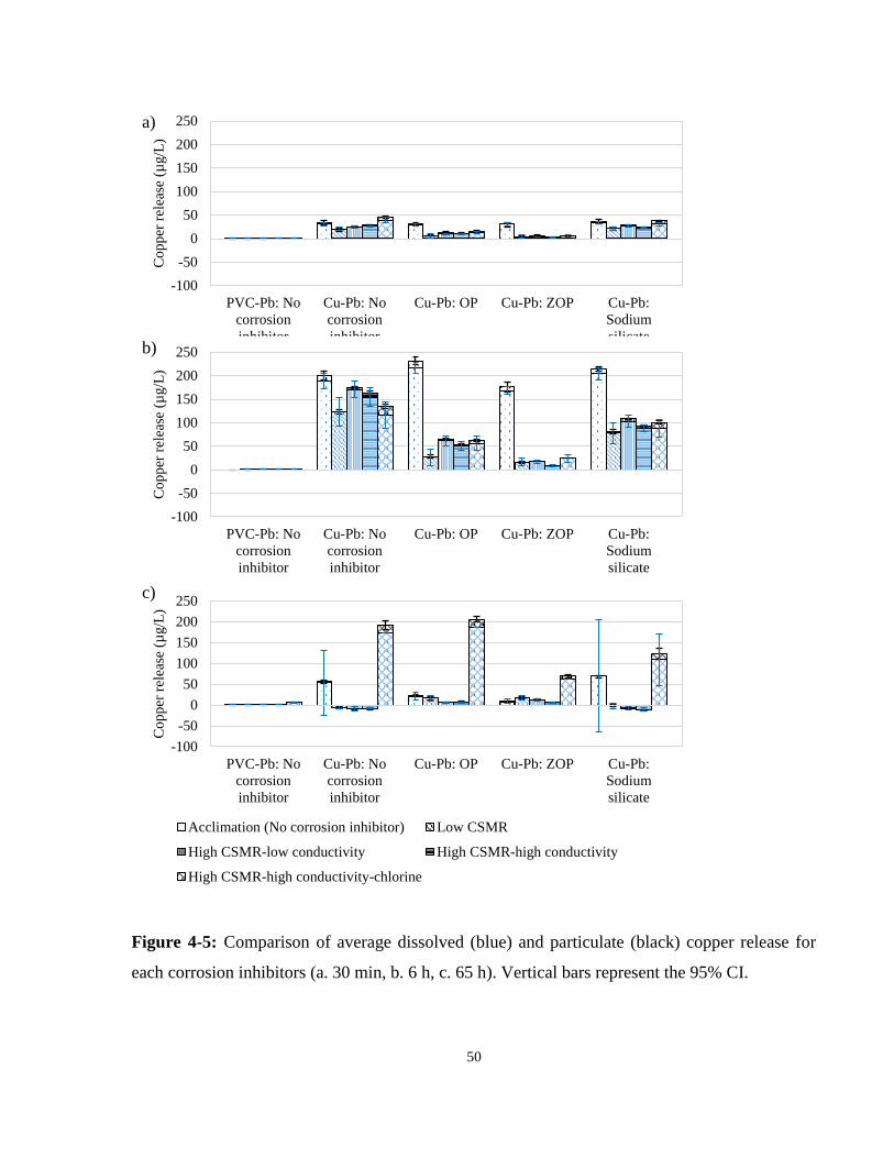
50

Figure 4-5: Comparison of average dissolved (blue) and particulate (black) copper release for

each corrosion inhibitors (a. 30 min, b. 6 h, c. 65 h). Vertical bars represent the 95% CI.

-100

-50

0

50

100

150

200

250

PVC-Pb: No

corrosion

inhibitor

Cu-Pb: No

corrosion

inhibitor


Sodium

silicate

Co

pp

er r

elea

se (

µg/L

)

-100

-50

0

50

100

150

200

250

PVC-Pb: No

corrosion

inhibitor

Cu-Pb: No

corrosion

inhibitor


Sodium

silicate

Co

pp

er r

elea

se (

µg/L

)

-100

-50

0

50

100

150

200

250

PVC-Pb: No

corrosion

inhibitor

Cu-Pb: No

corrosion

inhibitor


Sodium

silicate

Co

pp

er r

elea

se (

µg/L

)



High CSMR-high conductivity-chlorine

b)

c)

a)

51

4.5 Conclusions

In this study, both ZOP and OP were observed to effectively decrease lead release following

application. Their performance was unaffected by changes in CSMR (0.2 and 1) or conductivity

(approximately 330 mS/cm and 550-570 mS/cm). In comparison, addition of sodium silicate did

not effectively decrease lead release. It should be noted however that sodium silicate did

significantly decrease lead after six months, corroborating evidence from other studies that

suggest that a longer surface passivation period is required. ZOP and OP provided significantly

greater decreases in both total and dissolved lead release when compared to sodium silicates.

Chlorine initially increased particulate lead release, but its presence decreased dissolved lead

release in most systems.

Similar observations were made for copper control, where both OP and ZOP provided significant

decreases following 30-min and 6-h stagnation times. Following 65-h stagnation, there was

evidence that copper deposition had occurred in both the corrosion inhibitor free control and

sodium silicate treated systems which have important implications for lead release. Mechanisms

of differences between inhibitor performances could be revealed by an autopsy analysis of pipe

scales and should be considered in future studies. Utilities operating systems where lead and

copper couplings occur (PLSLR) should consider the impact of the corrosion control strategy on

copper control. This research highlights the complex interplay of corrosion inhibitor, metal

fractions (particulate or dissolved), stagnation time and copper deposition on the management of

lead and copper release from PLSLR.

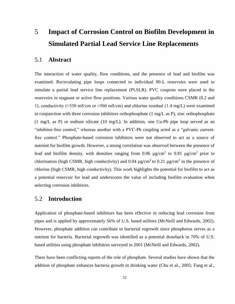
52

5 Impact of Corrosion Control on Biofilm Development in

Simulated Partial Lead Service Line Replacements

5.1 Abstract

The interaction of water quality, flow conditions, and the presence of lead and biofilm was

examined. Recirculating pipe loops connected to individual 90-L reservoirs were used to

simulate a partial lead service line replacement (PLSLR). PVC coupons were placed in the

reservoirs in stagnant or active flow positions. Various water quality conditions CSMR (0.2 and

1), conductivity (≈330 mS/cm or ≈560 mS/cm) and chlorine residual (1.4 mg/L) were examined

in conjunction with three corrosion inhibitors orthophosphate (1 mg/L as P), zinc orthophosphate

(1 mg/L as P) or sodium silicate (10 mg/L). In addition, one Cu-Pb pipe loop served as an

“inhibitor-free control,” whereas another with a PVC-Pb coupling acted as a “galvanic current-

free control.” Phosphate-based corrosion inhibitors were not observed to act as a source of

nutrient for biofilm growth. However, a strong correlation was observed between the presence of

lead and biofilm density, with densities ranging from 0.06 µg/cm2 to 0.81 µg/cm2 prior to

chlorination (high CSMR, high conductivity) and 0.04 µg/cm2 to 0.21 µg/cm2 in the presence of

chlorine (high CSMR, high conductivity). This work highlights the potential for biofilm to act as

a potential reservoir for lead and underscores the value of including biofilm evaluation when

selecting corrosion inhibitors.

5.2 Introduction

Application of phosphate-based inhibitors has been effective in reducing lead corrosion from

pipes and is applied by approximately 56% of U.S. based utilities (McNeill and Edwards, 2002).

However, phosphate addition can contribute to bacterial regrowth since phosphorus serves as a

nutrient for bacteria. Bacterial regrowth was identified as a potential drawback in 70% of U.S.

based utilities using phosphate inhibitors surveyed in 2001 (McNeill and Edwards, 2002).

There have been conflicting reports of the role of phosphate. Several studies have shown that the

addition of phosphate enhances bacteria growth in drinking water (Chu et al., 2005; Fang et al.,

53

2009; Payne et al., 2016; Lehtola et al., 2002); whereas in other cases phosphate was not

observed to enhance bacteria growth (Batté et al., 2003b). Chu et al. (2005) reported

heterotrophic plate counts (HPCs) in biofilm to reach a stable level (2.47×105 CFU/cm2) after 6

weeks and significantly increase to 1.04×106 CFU/cm2 following the addition of 0.01 mg P/L

phosphate, but the increasing phosphate dose to 0.05 did not result in a further increase. Fang et

al. (2009) reported addition of 30 and 300 µg/L of phosphorus to decrease exopolysaccharide

(EPS) production by 81% and 77%, respectively. However, after 15 and 30 days, addition of 30

and 300 µg/L of phosphorus increased the biofilm cell metabolic potential by seven and eight

fold to 70.89 and 67.96 MPI (metabolic potential index). Payne et al. (2016) observed that 3 mg-

PO4/L resulted in significantly higher biofilm on PVC coupons compared to a control in lead and

copper impacted environments. The same authors reported phosphate addition to increase

biofilm community diversity, which has been demonstrated to have important implications for

disinfection effectiveness by Simões et al. (2010).

The role of surface area on biofilm growth has been implied in several studies (Camper et al.,

2003; Ollos et al., 2003; Payne, 2013). Recent studies have demonstrated that zinc

orthophosphate treated lead systems are dominated by particles, compared to dissolved species

(Cartier et al., 2012b; Camara et al., 2013; Woszczynski et al., 2013). It is hypothesized that

increased particles, could act to increase available surface area for biofilm growth, thus

increasing biofilm density. In contrast, silicate is not a major nutrient for bacteria and as such

does not contribute to bacterial regrowth in drinking water distribution systems.

This study explored the complex interrelationship of lead particles, biofilm growth, the absence

and presence of chlorine, and corrosion inhibitor type (orthophosphate, zinc orthophosphate and

sodium silicate).

54

5.3 Materials and Methods

5.3.1 Partial lead service line setup

Partial lead service line replacement was simulated using aged lead pipes which were harvested

following 63 years of service from a city located in Ontario, Canada. Lead pipes (internal

diameter 1.28±0.3 cm) used in this study were cut into 0.5 m sections and were coupled with 0.5

m sections of new copper pipes (internal diameter 1.27 cm). Insulating plastic spacers were

placed between the copper and lead pipes. The two pipe materials were connected via an external

copper wire placed 7 cm from the junction to create an external and measurable galvanic current.

Periods of the acclimation and subsequent corrosion inhibitor trials (Table 5-1) were conducted

under alternating stagnant and flow-through conditions using a recirculation system (Figure 3-1).

To facilitate biofilm collection, polycarbonate coupons (approximate surface area 45 cm2; length

15 cm) subjected to stagnant conditions were inserted in each reservoir. Coupons subjected to

flow-through conditions were connected to the effluent of pipe loops.

Recirculating pipe loops were connected to 90-L reservoirs holding Lake Ontario water (Table

5-2), which allowed for one complete daily flush of the system with fresh water, given 120 min

of flow per day. Recirculating pumps provided flow in all pipe loops. Timers were programmed

to simulate a flow rate of 5 L/min for a total 120 min of flow (600 L/day for typical household)

with alternating stagnation periods ranging from 10 min to 8 h 20 min. To serve a control for

biofilm analysis, a similar system with a 50-L reservoir and PVC pipe sections was used.

55

Table 5-1: Experimental conditions for both acclimation and corrosion inhibitor trials (OP, ZOP, and sodium silicate)

Phase Experimental

period (weeks)

Galvanic

current CSMR

Conductivity

(mS/cm)

Chlorine residual

(mg/L)

Number of biofilm samples collected

ATP Pb and Cu

Acclimation 4 No 0.2 NM 0 0 0

Low CSMR 12 Yes 0.2 550 0 4 0

High CSMR-low

conductivity 6 Yes 1 330 0 2 0

High CSMR-high

conductivity 8 Yes 1 570 0 2 2

High CSMR-high

conductivity-

chlorine

13 Yes 1 600 1.4 8 8

56

Table 5-2: Raw water quality

Parameter (unit) Average (± standard deviation)

pH 7.9±0.1

Turbidity (NTU) 0.607±0.580

Alkalinity (mg/L as CaCO3) 91.4 ±1.0

TOC (mg/L) 2.3±0.3

Nitrate (mg/L) 1.56±0.24 mg/L

Nitrite (mg/L) <MDL (0.57 mg/L)

Phosphate (mg/L as P) <MDL (0.04 mg/L)

Silicate (mg/L as SiO2) 1.5 ±0.3

ATP (ng/100 mL) 0.06±0.02

5.3.2 Experimental plan

Following 4 weeks of acclimation (Table 5-1), a galvanic connection was installed between the

lead and copper pipes using an external copper wire and maintained during four “treatment”

phases of low CSMR, high CSMR-low conductivity, high CSMR-high conductivity, and high

CSMR-high conductivity-chlorine. Three corrosion inhibitors were added during the treatment

phases: sodium orthophosphate (OP) 1 mg P/L (Sigma-Aldrich Co.), zinc orthophosphate (ZOP)

1 mg P/L (Carus Co., LaSalle, IL), and sodium silicate 10 mg/L (National Silicates, Toronto,

ON, Canada).

A 42-day biofilm development period was used, consistent with previous studies (Gagnon et al.,

2004, 2005; Rand et al., 2007; Payne et al., 2016). One set of polycarbonate coupons under

stagnant and flow-through conditions was collected from each reservoirs and used for ATP

analysis. During phases with high CSMR-high conductivity and high CSMR-high conductivity-

chlorine conditions, each coupon was cut in half; one piece was used for ATP analysis and the

other for analysis of lead accumulating in biofilm.

5.3.3 Sample Analysis

5.3.3.1 Analysis of water quality parameters

A laboratory pH meter (Model 8015, VWR Scientific Inc., Mississauga, ON) was used to

determine pH. Concentrations of chloride, sulfate, and phosphate were measured using ion

chromatography (IC) with a Dionex ICS-5000 system (Thermo Scientific, Sunnyvale, CA)

57

according to the U.S. EPA Method 300.0 (Pfaff, 1993). Silica and free chlorine were determined

using a HACH silicomolybdate Method (8185) and the DPD colorimetric method described in

Standard Method 4500-Cl- (APHA et al., 2005), respectively, with a DR 2700 Portable

Spectrophotometer (HACH Co., Loveland, CO). Total organic carbon (TOC) was analyzed using

a Model 1010 Wet Oxidation TOC Analyzer with a Model 1051 Vial Multi-Sampler (O.I.

Analytical, College Station, TX) based on a wet oxidation method as described in Standard

Method 5310 D (APHA et al., 2005). Alkalinity was measured using an end-point colorimetric

titration procedure based on Standard Method 2320 B (APHA et al., 2005). Galvanic current

flowing from the lead to the copper pipes was measured by a multi-meter (Model #22-811,

RadioShack, Fort Worth, TX) with 100-Ω resistance based on the method used by Nguyen et al.

(2011b). The external copper wire connecting the two pipes was removed and replaced with the

multi-meter for 30 sec to obtain readings. Conductivity was monitored using a sensION+

MM150 portable Multi-parameter meter (HACH Co., Loveland, CO).

5.3.3.2 Analysis of ATP

Adenosine triphosphate (ATP) in biofilm and raw water samples were determined by using

Quench-GoneTM Aqueous test kits and Deposit and Surface Analysis test kits (LuminUltra

Technologies Ltd., Fredericton, NB), respectively, with a pre-calibrated luminometer

(LuminUltra Technologies Ltd., Fredericton, NB). Half of each coupons was used for ATP

analysis for biofilm, leaving the left for lead and copper analyses.

5.3.3.3 Analysis of dissolved and total lead in biofilm

To analyze dissolved and total lead in biofilm, half of the coupons were collected from the six

reservoirs. Biofilm was removed from both sides of a collected coupon by a clean disposable

lead-free scraper into a clean 15-mL polypropylene tube. All biofilm on each coupon was

obtained by rinsing any remaining biofilm with Milli-Q water. The volume of the solution was

adjusted to 30 mL, and all samples were mixed thoroughly. For dissolved lead analysis, half of

each sample was filtered using a 0.45-µm syringe filer, discarding the first 5 mL of filtrate. To

capture the total lead, including the particulate portion, the remaining sample and coupons were

prepared using nitric acid digestion at 105º C for 2 h (Standard Method 3030 E, APHA et al.,

2005). For both dissolved and total lead samples, 0.25% (v/v) nitric acid was added to pH <2

according to Standard Method 3030 B (APHA et al., 2005) for preservation and stored at 4º C

58

until analysis using ICP-AES. Method detection limit for lead and copper were 6.0 and 5.7 µg/L,

respectively.

5.3.4 Estimation of lead released through galvanic current

The theoretical amount of lead released through galvanic currents was estimated using Faraday’s

law (Dudi, 2004).

5.3.5 Statistical Analysis

Confidence intervals were used for comparison of treatments. All statistical analyses were

conducted at the 95% confidence level (Berthouex and Brown, 2002).

5.4 Results and Discussion

5.4.1 Effects of corrosion inhibitors on biofilm growth under stagnant and

flow-through conditions

Biofilm on polycarbonate coupons under stagnant and flow-through conditions (Figure 3-1) was

measured to determine the impact of corrosion inhibitors and flow conditions on microbial

growth (Figure 5-1). In general, prior to chlorination, biofilm growth under stagnant conditions

tended to have higher ATP densities when compared to flow-through conditions, with the OP

system having the highest ATP during the high CSMR high conductivity trial. Under flow

conditions, prior to chlorination, ZOP had significantly higher ATP counts for the low CSMR

and high CSMR high conductivity trials.

Chlorination significantly decreased ATP densities in all systems. A 0.9 to 2.2 and 1.0 to 2.0-log

reduction was observed under stagnant condition and flow-through condition, respectively (Table

5-3). Notably, the biofilm was more resistant to disinfection when considering flow through

conditions. Biofilm cohesiveness has been reported to increase after exposure to shear stress (0.2

Pa-10 Pa), Mathieu et al. (2014), consistent with observations by others that biofilm volumetric


coulombs

)×t(s)×207.2g Pb

mole Pb

1.6×10-19(coulomb

e)×6.023×1023(

Pbmole Pb

)×2(e

Pb)

5-1

59

density increases under higher flow velocities (Garny et al., 2008). Lehtola et al. (2006) also

observed an increase in biofilm with increasing flow rate for both copper and plastic pipes. Ollos

et al. (2003) compared two levels of shear stress (0.4 and 2.0 N/m2) and suggested lower shear

stress (or flow) may limit biofilm accumulation by reducing mass transfer of biodegradable

organic matter.

The presence of particles may also play a role in biofilm accumulation by creating more

available surface area for growth. A correlation between lead trapped in the biofilm for the high

CSMR-high conductivity and the high CSMR-high conductivity-chlorine were compared (Figure

5-2); positive correlations were observed for all systems where lead was available.

Lead accumulating in biofilm was measured to determine the effect of corrosion inhibitors. For

all systems containing lead pipes, approximately 96-99% and 96-99% of lead accumulating in

biofilm under stagnant and flow-through conditions, respectively, was in the form of particulate

for non-chlorinated-high CSMR-high conductivity condition (Table 5-4). In the presence of

chlorine, the amount of lead accumulation decreased with the inactivation and detachment of

biofilm. Approximately 85-98% and 92-98% of lead stored in biofilm under stagnant and flow-

through conditions was of particulate form in the chlorinated water.

Typically, trends of ATP and lead accumulation were consistent, suggesting that the density of

biofilm impacted lead storage capacity (Figure 5-1; Figure 5-3). Higher amounts of lead

accumulating in stagnant biofilm were observed for the systems with higher ATP densities under

non-chlorinated conditions, such as the corrosion inhibitor-free Cu-Pb, OP, and sodium silicate

systems. When considering non-chlorinated flow-through conditions, the highest lead

accumulation was observed in the ZOP system, consistent with the highest ATP density. Under

chlorinated condition, the average ATP and lead accumulation were less correlated. The biofilm

under flow-through condition in the ZOP system stored a larger amount of lead both in non-

chlorinated and chlorinated conditions, when compared to other systems. While the average ATP

densities were similar for all systems, the amounts of lead remained high only in the ZOP system

for chlorinated flow-through trial. The ZOP system released more lead particles due to the

apparent effect of ZOP (Payne 2013; Woszczynski et al, 2013) and entrapped them in biofilm

during flow. In contrast, the phosphate-enriched OP system had low accumulation even though it

had the second highest ATP density. Systems with greater ATP densities tended to have better

60

correlations with lead accumulation. Past studies have reported systems with ductile iron to have

greater HPCs than systems with plastic pipes when considering a range of chlorine

concentrations (Camper et al., 2003) and carbon levels (Ollos et al., 2003). The same researchers

hypothesized that surface area played a role. Accumulation of lead particles in biofilm increased

surface area, and it is plausible that the presence of lead particles in biofilm conversely affected

microbial growth. Similarly, total copper was also observed to accumulate in biofilm (Figure 5-4;

Figure 5-5) with positive correlations between ATP and copper accumulation.

The ability of phosphate to serve as a nutrient was also examined. Comparison to a phosphate-

free sodium silicate system did not reveal any clear trends (Figure 5-1). Rompré et al. (2000)

reported that the mass of biofilm was not significantly different in phosphate systems when

compared to sodium silicate treated systems and concluded that the surface was a key factor

influencing biofilm development. In this study, phosphate does not act as a nutrient. Batté et al.

(2003a) observed that P addition did not enhance biofilm growth in a carbon limited

environment, and the authors deduced that the added P was stored in the extracellular matrix of

the biofilm.

Table 5-3: Log reduction in ATP in stagnant and flow-through biofilm by chlorination

System Log reduction

Stagnant Flow-through

PVC-PVC: No corrosion inhibitor 0.9 1.0

PVC-Pb: No corrosion inhibitor 1.3 1.2

Cu-Pb: No corrosion inhibitor 2.0 1.3

Cu-Pb: OP 2.2 1.5

Cu-Pb: ZOP 1.3 2.0

Cu-Pb: Sodium silicate 2.0 1.3

61

Figure 5-1: ATP accumulation under a) stagnant and b) flow-through conditions. n=4, 2, 2, and

8 for low CSMR, high CSMR-low conductivity, high CSMR-high conductivity, and high

CSMR-high conductivity-chlorine phases. Vertical bars represent 95% CI.

0.0

1.0

2.0

3.0

Low CSMR High CSMR-low

conductivity

High CSMR-high

conductivity

High CSMR-high


Lo

g1

0 (

AT

P n

g/c

m2)

0.0

1.0

2.0

3.0

Low CSMR High CSMR-low

conductivity

High CSMR-high

conductivity

High CSMR-high


Lo

g1

0 (

AT

P n

g/c

m2)

PVC-PVC: No corrosion inhibitor PVC-Pb: No corrosion inhibitor

Cu-Pb: No corrosion inhibitor Cu-Pb: OP

Cu-Pb: ZOP Cu-Pb: Sodium silicate

a)

b)

62

Figure 5-2: Total lead and ATP accumulation under a) stagnant and b) flow-through conditions

(linear regression). n=10.

R² = 0.1582

R² = 0.9523R² = 0.9756

R² = 0.9379

R² = 0.8101

0.0

0.5

1.0

1.5

2.0

2.5

3.0

0.00 0.20 0.40 0.60 0.80 1.00

AT

P (

ng/c

m2)

Total lead in biofilm (µg/cm2)

R² = 0.9056R² = 0.8579

R² = 0.503

R² = 0.8309R² = 0.5663

0.0

0.5

1.0

1.5

2.0

2.5

3.0

0.00 0.20 0.40 0.60 0.80 1.00

AT

P (

ng/c

m2)

Total lead in biofilm (µg/cm2)




b)

a)

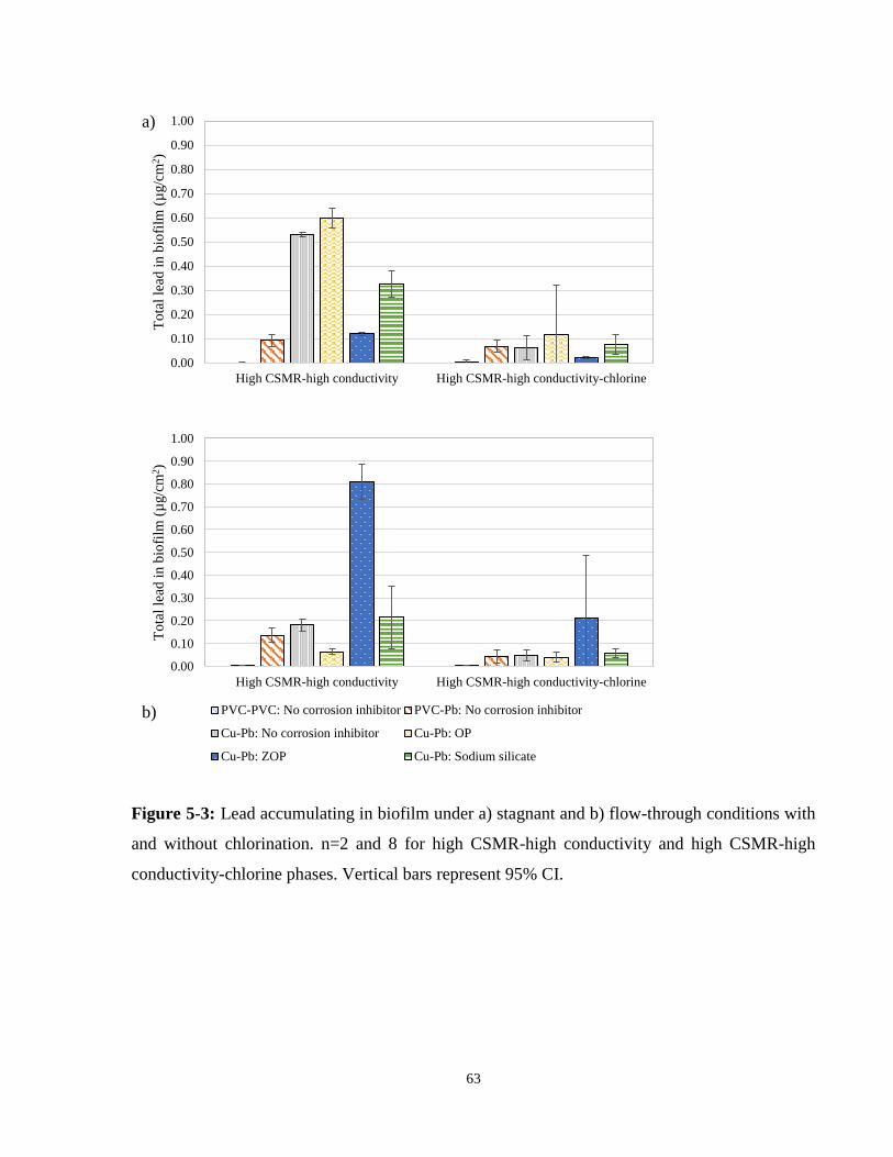
63

Figure 5-3: Lead accumulating in biofilm under a) stagnant and b) flow-through conditions with

and without chlorination. n=2 and 8 for high CSMR-high conductivity and high CSMR-high

conductivity-chlorine phases. Vertical bars represent 95% CI.

0.00

0.10

0.20

0.30

0.40

0.50

0.60

0.70

0.80

0.90

1.00

High CSMR-high conductivity High CSMR-high conductivity-chlorine

To

tal

lead

in b

iofi

lm (

µg/c

m2)

0.00

0.10

0.20

0.30

0.40

0.50

0.60

0.70

0.80

0.90

1.00


To

tal

lead

in b

iofi

lm (

µg/c

m2)




b)

a)

64


with and without chlorination. n=10.

R² = 0.4804

R² = 0.9869R² = 0.991

R² = 0.8571

R² = 0.9771

0.0

0.5

1.0

1.5

2.0

2.5

3.0

0.00 0.20 0.40 0.60 0.80 1.00

AT

P (

ng/c

m2)

Total copper in biofilm (µg/cm2)

R² = 0.8774 R² = 0.7547

R² = 0.8494 R² = 0.8891

R² = 0.5671

0.0

0.5

1.0

1.5

2.0

2.5

3.0

0.00 0.20 0.40 0.60 0.80 1.00

AT

P (

ng/c

m2)

Total copper in biofim (µg/cm2)




b)

a)

65


with and without chlorination. n=2 and 8 for high CSMR-high conductivity and high CSMR-

high conductivity-chlorine phases. Vertical bars represent 95% CI.

0.00

0.10

0.20

0.30

0.40

0.50

0.60

0.70

0.80

0.90

1.00


To

tal

cop

per

in b

iofi

lm (

µg/c

m2)

0.00

0.10

0.20

0.30

0.40

0.50

0.60

0.70

0.80

0.90

1.00


To

tal

cop

per

in b

iofi

lm (

µg/c

m2)




66

Table 5-4: Particulate lead fraction in biofilm and bulk water (at the end of a weekly cycle)

Particulate fraction in total lead (%)

Acclimation Low CSMR High CSMR-

low

conductivity

High CSMR-

high

conductivity

High CSMR-

high

conductivity-

chlorine

Weekly lead

release in bulk

water

PVC-PVC: No corrosion inhibitor - - - - -

PVC-Pb: No corrosion inhibitor 12 20 35 19 24

Cu-Pb: No corrosion inhibitor 10 19 22 17 21

Cu-Pb: OP 11 47 69 41 48

Cu-Pb: ZOP 9 74 85 80 81

Cu-Pb: Sodium silicate 17 34 28 17 26

Stagnant

biofilm

PVC-PVC: No corrosion inhibitor - - - - 75

PVC-Pb: No corrosion inhibitor - - - 96 95

Cu-Pb: No corrosion inhibitor - - - 98 96

Cu-Pb: OP - - - 99 98

Cu-Pb: ZOP - - - 98 85

Cu-Pb: Sodium silicate - - - 99 96

Flow-through

biofilm

PVC-PVC: No corrosion inhibitor - - - 84 73

PVC-Pb: No corrosion inhibitor - - - 98 92

Cu-Pb: No corrosion inhibitor - - - 98 98

Cu-Pb: OP - - - 96 92

Cu-Pb: ZOP - - - 99 96

Cu-Pb: Sodium silicate - - - 99 96

The dash (-) refers to the results which samples were not collected or no lead was detected in the samples.

67

5.4.2 Estimation of capacity of biofilm for storing lead

During the initial weeks of chlorination, total lead release increased in the bulk water. This may

be partially attributed to release of biofilm containing lead particles. The capacity of biofilm for

storing lead was estimated based on observed ATP and lead densities for the flow-through

system, and an approximate wetted surface area of the pipe section. It was assumed that ATP and

lead densities in biofilm were similar throughout the system.

At the end of the high CSMR-high conductivity trial, 0.3-1.7% of the theoretical cumulative

mass release of lead was accumulated in the biofilm: 0.3, 0.1, 1.7, and 0.3% was observed for the

inhibitor free control, OP, ZOP, and sodium silicate (Table 5-5). Biofilm densities were

significantly lower for chlorinated water (Figure 5-1; Table 5-5). The biomass was estimated to

contain only 0.0-0.3% of theoretically released lead.

The capacity of biofilm to sorb lead is an important consideration as biofilm can be mobilized

during disinfection, physical disturbances. In order to quantify the impact biofilm associated

lead, estimates were made for a theoretical pipe (1 m long, 1cm diameter) under flow conditions

using lead-biofilm densities observed in this study (Table 5-5). Based on a 1m pipe (1 cm

diameter), the lead capacity prior to chlorination (high CSMR-high conductivity ranged from

20.1 to 254.5 µg. Following chlorination, the lead capacity ranged from 12.4 to 66.2 µg. Lehtola

et al. (2006) observed that copper concentrations increased in bulk water following periods of

flow, attributing it to detached biofilm. Similarly, Ginige et al. (2011) reported that biofilm

inactivation can release trapped Fe and Mn in biofilm, resulting in increased Mn concentrations.

Thus, the capacity of biofilm to act as a reservoir for lead is important, as detached biofilm could

potentially release a significant quantity of lead.

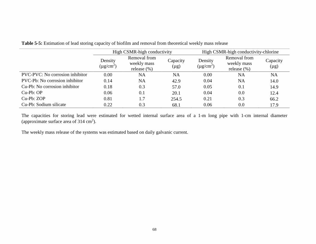
68

Table 5-5: Estimation of lead storing capacity of biofilm and removal from theoretical weekly mass release


Density

(µg/cm2)

Removal from

weekly mass

release (%)

Capacity

(µg)

Density

(µg/cm2)

Removal from

weekly mass

release (%)

Capacity

(µg)

PVC-PVC: No corrosion inhibitor 0.00 NA NA 0.00 NA NA

PVC-Pb: No corrosion inhibitor 0.14 NA 42.9 0.04 NA 14.0

Cu-Pb: No corrosion inhibitor 0.18 0.3 57.0 0.05 0.1 14.9

Cu-Pb: OP 0.06 0.1 20.1 0.04 0.0 12.4

Cu-Pb: ZOP 0.81 1.7 254.5 0.21 0.3 66.2

Cu-Pb: Sodium silicate 0.22 0.3 68.1 0.06 0.0 17.9

The capacities for storing lead were estimated for wetted internal surface area of a 1-m long pipe with 1-cm internal diameter

(approximate surface area of 314 cm2).

The weekly mass release of the systems was estimated based on daily galvanic current.

69

5.5 Conclusion

This study examined the impacts of various water quality and flow conditions, corrosion

inhibitors and chlorine disinfectant on biofilm growth and lead accumulation in biofilm. In this

study, the phosphate-based corrosion inhibitors (ZOP, OP) were not observed to act as a nutrient,

as in this water type microbial growth was likely limited by carbon. There was, however, a

strong correlation between the presence of lead and ATP, suggesting that lead particles may

provide surface area for biofilm growth. The results also suggest that biofilm could represent a

significant reservoir for lead storage and subsequent release. This work highlights the potential

for biofilm to act as a potential reservoir for lead, which could be released under changing water

quality conditions, and underscores the value of including biofilm assessment when selecting

corrosion inhibitors.

70

6 References

American Public Health Association (APHA), American Water Works Association (AWWA),

and Water Environment Federation (WEF). (2005) Standard methods for the examination

of water and wastewater, twenty first ed. (Washington, DC, USA).

Berthouex, P.M. and Brown, L.C. (2002) Statistics for Environmental Engineers. 2nd Edition.

CRC Press, Boca Raton, Florida

Batté, M., Koudjonou, B., Laurent, P., Mathieu, L., Coallier, J., and Prévost, M. (2003a) Biofilm

responses to ageing and to a high phosphate load in a bench-scale drinking water system.

Water Research 37, 1351-1361.

Batté, M., Mathieu, L., Laurent, P., and Prévost, M. (2003b) Influence of phosphate and

disinfection on the composition of biofilms produced from drinking water, as measured

by fluorescence in situ hybridization. Canadian Journal of Microbiology 49, 741-753.

Boyd, G.R., Dewis, K.M., Korshin, G.V., Reiber, S.H., Schock, M.R., and Sandvig, A.M. (2008)

Effects of changing disinfectants on lead and copper release. Journal American Water

Works Association 100 (11), 75-87.

Boyd, G.R., Shetty, P., Sandvig, A.M., and Pierson G.L. (2004) Pb in tap water following

simulated partial lead pipe replacements. Journal of environmental Engineering 130,

1188-1197.

Brown, M.J., Raymond, J., Homa, D., Kennedy, C., and Sinks, T. (2011) Association between

children’s blood lead levels, lead service lines, and water disinfection, Washington, DC,

1998-2006. Environmental Research 111, 67-74.

Camara, E., Montreuil, K.R., Knowles, A.K., and Gagnon, G.A. (2013) Role of the water main in

lead service line replacement: a utility case study. Journal American Water Works

Association 105 (8), E423-E431.

71

Camper, A.K., Brastrup, K., Sandvig A., Clement, J., Spencer C., and Capuzzi A.J. (2003) Effect

of distribution system materials on bacterial regrowth. Journal American Water Works

Association 95 (7), 107-121.

Cantor, A.F., Park, J.K., and Vaiyavatjamai, P. (2003) Effect of chlorine on corrosion in drinking

water systems. Journal American Water Works Association 95 (5), 112-123.

Cardew, P.T. (2009) Measuring the benefit of orthophosphate treatment on lead in drinking

water. Journal of Water and Health 7 (1), 123-131.

Cartier, C., Laroche, L., Deshommes, E., Nour, S., Richard, G., Edwards, M., and Prévost, M.

(2011) Investigating dissolved lead at the tap using various sampling protocols. Journal

American Water Works Association 103 (3), 55-67.

Cartier, C., Arnold, R.B., Triantafyllidou, S., Prévost, M., and Edwards, M. (2012a) Effect of

flow rate and lead/copper pipe sequence on lead release from service lines. Water

Research 46 (13), 4142-4152.

Cartier, C., Nour, S., Richer, B., Deshommes, E., and Prévost, M. (2012b) Impact of water

treatment on the contribution of faucets to dissolved and particulate lead release at the

tap. Water Research 46, 5205-5216.

Cartier, C., Doré, E., Laroche, L., Nour, S., Edwards, M., and Prévost, M. (2013) Impact of

treatment on Pb release from full and partially replaced harvested lead service lines

(LSLs). Water Research 47 (2), 661-671.

Chu, C., Lu, C., and Lee, C. (2005) Effects of inorganic nutrients on the regrowth of

heterotrophic bacteria in drinking water distribution systems. Journal of Environmental

Management 74, 255-263.

Churchill, D.M., Mavinic, D.S., Neden, D.G., and MacQuarrie, D.M. (2000) The effect of zinc

orthophosphate and pH-alkalinity adjustment on metal levels leached into drinking water.

Canadian Journal of Civil Engineering 27, 33-43.

72

Clark, B., Cartier, C., St. Clair, J., Triantafyllidou, S., Prévost, M., Edwards, M. 2013. Effect of

connection type on galvanic corrosion between lead and copper pipes. Journal American

Water Works Association 105(10), E576-E586.

Clark, B., Masters, S., and Edwards, M. (2014) Profile sampling to characterize particulate lead

risks in potable water. Environmental Science & Technology 48, 6836-6843.

Clark, B., St. Clair, J., and Edwards, M. (2015) Copper deposition corrosion elevated lead release

to potable water. Journal American Water Works Association 107 (11), E627-E637.

Dart, J.F. and Foley, P.D. (1970) Preventing iron deposition with sodium silicate. Journal


Dartmann, J., Sadlowsky, B., Dorsch, T., and Johannsen, K. (2010) Copper corrosion in drinking

water systems – effect of pH and phosphate-dosage. Materials and Corrosion 61 (3), 189-

198.

Del Toral, M.A., Porter, A., and Schock, M.R. (2013) Detection and evaluation of elevated lead

release from service lines: a field study. Environmental Science & Technology 47(16),

9300-9307.

Deshommes, E. and Prévost, M. (2012) Pb particles from tap water: bioaccessibility and

contribution to child exposure. Environmental Science & Technology 46, 6269-6277.

Dodrill, D.M. and Edwards, M. (1995) Corrosion control on the basis of utility experience.

Journal American Water Works Association 87, 74-85.

Dudi, A. (2004) Reconsidering lead corrosion in drinking water: product testing, direct

chloramine attack and galvanic corrosion (MSc. thesis). Virginia Polytechnic Institute:

Blacksburg, VA, USA.

Edwards, M., Jacobs, S., and Dodrill, D. (1999) Desktop guidance for mitigating Pb and Cu

corrosion by-products. Journal: American Water Works Association 91 (5), 66-77.

73

Edwards, M. and Dudi, A. (2004). Role of chlorine and chloramine in corrosion of lead-bearing

plumbing materials. Journal American Water Works Association 96 (10), 69-81.

Edwards, M., Hidmi, L., and Gladwell, D. (2002) Phosphate inhibition of soluble copper

corrosion by-product release. Corrosion Science 44 (5), 1057-1071.

Edwards, M. and McNeill, L.S. (2002) Effect of phosphate inhibitors on lead release from pipes.

Journal American Water Works Association 94 (1), 79-90.

Edwards, M.A. and Triantafyllidou, S. (2007) Chloride-to-sulfate mass ratio and lead leaching to

water. Journal American Water Works Association 99 (7), 96- 109.

Environment and Climate Change Canada (2011) Residential water use in Canada.

https://www.ec.gc.ca/indicateurs-indicators/default.asp?lang=en&n=7E808512-1

(accessed June 2016)

Fang, W., Hu, J.Y., and Ong, S.L. (2009) Influence of phosphorus on biofilm formation in model

drinking water distribution systems. Journal of Applied Microbiology 106, 1328-1335.

Gagnon, G.A. and Doubrough J.D. (2011) Lead release from premise plumbing: a profile of

sample collection and pilot studies from a small system. Canadian Journal of Civil

Engineering 38, 741-750.

Gagnon, G.A., O’Leary, K.C., Volk, C.J., Chauret, C., Stover, L., and Andrews, R.C. (2004)

Comparative analysis of chlorine dioxide, free chlorine and chloramines on bacterial

water quality in model distribution systems. Journal of Environmental Engineering 130

(11), 1269-1279.

Gagnon, G.A., Rand, J.L., O’Leary, K.C., Rygel, A.C., Chauret, C., and Andrews, R.C. (2005)

Disinfectant efficacy of chlorite and chlorine dioxide in drinking water biofilms. Water

Research 39 (9), 1809-1817.

Garny, K., Horn, H., and Neu, T.R. (2008) Interaction between biofilm development, structure

and detachment in rotating annular reactors. Bioprocess and Biosystems Engineering 31,

619-629.

https://www.ec.gc.ca/indicateurs-indicators/default.asp?lang=en&n=7E808512-1

74

Ginige, M.P., Wylie, J., and Plumb, J. (2011) Influence of biofilms on iron and manganese

deposition in drinking water distribution systems. Biofouling 27 (2), 151-163.

Gregory, R. (1985) Galvanic corrosion of lead in copper pipework: phase I, measurement of

galvanic corrosion potential in selected waters. Water Research Centre Engineering.

Swindon, England.

Hu, J., Gan, F., Triantafyllidou, S., Nguyen, C.K., and Edwards, M.A. (2012) Copper-induced

metal release from lead pipe into drinking water. Corrosion 68 (11), 1037-1048.

Health Canada (2007) Water talk: minimizing exposure to lead from drinking water distribution

systems. http://www.hc-sc.gc.ca/ewh-semt/pubs/water-eau/lead-plomb-eng.php (accessed

March 2016).

Health Canada (2013) Final Human Health State of the Science Report of Lead. http://www.hc-

sc.gc.ca/ewh-semt/pubs/contaminants/dhhssrl-rpecscepsh/index-eng.php (accessed July

2016).

Hozalski, R.M., Esbri-Amador, E., and Chen, C.F. (2005) Comparison of stannous chloride and

phosphate for lead corrosion control. Journal: American Water Works Association 97 (3),

89-103.

Hu, J., Gan, F., Triantafyllidou, S., Nguyen, C.K., and Edwards, M.A. (2012) Copper-induced

metal release from lead pipe into drinking water. Corrosion 68 (11), 1037-1048.

Kennedy, C., Yard, E., Dignam, T., Buchanan, S., Condon, S., Brown M.J., Raymond J., Rogers,

H.S., Sarisky, J., de Castro R., Arias, I., and Breysse, P. (2016) Blood Lead Levels

Among Children Aged <6 Years — Flint, Michigan, 2013–2016. Morbidity and

Mortality Weekly Report. ePub: 24 June 2016. DOI:

http://dx.doi.org/10.15585/mmwr.mm6525e1 (accessed July, 2016).

Kim, E.J. and Herrera, J.E. (2010) Characteristics of lead corrosion scales formed during

drinking water distribution and their potential influence on the release of lead and other

contaminants. Environmental Science & Technology 44, 6054-6061.

http://www.hc-sc.gc.ca/ewh-semt/pubs/water-eau/lead-plomb-eng.php

http://www.hc-sc.gc.ca/ewh-semt/pubs/contaminants/dhhssrl-rpecscepsh/index-eng.php

http://www.hc-sc.gc.ca/ewh-semt/pubs/contaminants/dhhssrl-rpecscepsh/index-eng.php

http://dx.doi.org/10.15585/mmwr.mm6525e1

75

Lehtola, M.J., Miettinen, I.T., and Martikainen, P.J. (2002) Biofilm formation in drinking water

affected by low concentrations of phosphorus. Canadian Journal of Microbiology 48,

4994-499.

Lehtola, M.J., Laxander, M., Miettinen, I.T., Hirvonen, A., Vartiainen, T., and Martikainen, P.J.

(2006) The effects of changing water flow velocity on the formation of biofilms and

water quality in pilot distribution system consisting of copper or polyethylene pipes.


Lintereur, P.A., Duranceau, S.J., Taylor, J.S., and Stone, E.D. (2010) Sodium silicate impacts on

lead release in a blended potable water distribution system. Desalination and Water

Treatment 16, 427-438.

Lytle, D.A. and Schock, M.R. (2000) Impact of stagnation time on metal dissolution from

plumbing materials in drinking water. Journal of Water Supply: Research and

Technology-AQUA 49 (5), 243-257.

Lytle, D.A. and Schock, M.R. (2005) Formation of Pb(IV) oxides in chlorinated water. Journal


Lytle, D.A., Schock, M.R., and Scheckel, K. (2009) The inhibition of Pb(IV) oxide formation in

chlorinated water by orthophosphate. Environmental Science & Technology 43, 6624-

6631.

MacQuarrie, D.M., Mavinic, D.S., and Neden, D.G. (1997) Greater Vancouver Water District

drinking water corrosion inhibitor testing. Canadian Journal of Civil Engineering 24, 34-

52.

Mathieu, L., Bertrand, I., Abe, Y., Angel, E., Block, J.C., Skali-Lami, S., and Francius, G. (2014)

Drinking water biofilm cohesiveness changes under chlorination or hydrodynamic stress.


McGill, S.M. (2012) ‘Peak’ phosphorous? The implications of phosphate scarcity for sustainable

investors. Journal of Sustainable Finance and Investment 2 (3-4), 222-239.

76

McNeill, L.S. and Edwards, M. (2002) Phosphate inhibitor use at US utilities. Journal American

Water Works Association 94 (7), 57-63.

McNeill, L.S. and Edwards, M. (2004) Importance of Pb and Cu particulate species for corrosion

control. Journal of Environmental Engineering 130, 136-144.

Murphy, H.M., Payne, S.J., Gagnon, G.A. (2008) Sequential UV- and chlorine-based

disinfection to mitigate Escherichia coli in drinking water biofilms. Water Research 42,

2083-2092.

Nguyen, C.K., Stone, K.R., Dudi, A., and Edwards, M.A. (2010) Corrosive Microenvironments

at lead solder surfaces arising from galvanic corrosion with copper pipe. Environmental

Science & Technology 44 (18), 7076-7081.

Nguyen, C.K., Clark, B.N., Stone, K.R., and Edwards, M.A. (2011a) Acceleration of galvanic

lead solder corrosion due to phosphate. Corrosion Science 53, 1515-1521.

Nguyen, C.K., Clark, B.N., Stone, K.R., and Edwards, M.A. (2011b) Role of chloride, sulfate,

and alkalinity on galvanic lead corrosion. Corrosion 67 (6), E1-9.

Nguyen, C.K., Stone, K.R., and Edwards, M.A. (2011c) Chloride-to-sulfate mass ratio: practical

studies in galvanic corrosion of lead solder. Journal American Water Works Association

103 (1), 81-92.

Noel, J.D., Wang, Y., and Giammar, D.E. (2014) Effect of water chemistry on the dissolution

rate of the lead corrosion product hydrocerussite. Water Research 54, 237-246.

Ollos, P.J., Huck, P.M., and Slawson, R.M. (2003) Factors affecting biofilm accumulation in

model distribution systems. Journal American Water Works Association 95 (1), 87-97.

Payne, S.J.O. (2013) Interactions of corrosion control and biofilm on lead and copper in premise

plumbing (Ph. D. dissertation). Dalhousie University, Halifax, Nova Scotia, Canada.

Payne, S., Piorkowski, G.S., Truelstrup Hansen, L., and Gagnon, G.A. (2016) Impact of zinc

orthophosphate on simulated drinking water biofilms influenced by lead and copper.

Journal of Environmental Engineering 142 (2), 04015067.

77

Pfaff, J.D. (1993) Method 300.0 Determination of inorganic anions by ion chromatography. U.S.

Environmental Protection Agency, Cincinnati, Ohio, USA.

Pinto, J.A., McAnally, A.S., and Flora, J.R. (1997) Evaluation of lead and copper corrosion

control techniques. Journal of Environmental Science and Health A 32 (1), 31-53.

Rand, J.L., Hoffman, R., Alam, M.Z.B., Chauret, C., Cantwell, R., Andrews, R.C., and Gagnon,

G. A. (2007) A field study evaluation for mitigating biofouling with chlorine dioxide or

chlorine integrated with UV disinfection. Water Research 41(9), 1939-1948.

Renner, R. (2010) Reaction to the solution: lead exposure following partial service line

replacement. Environmental. Health Perspectives A202-A208.

Robinson B.R., Minear, R.A., and Holden J.M. (1992) Effects of Several Ions on iron treatment

by sodium silicate and hypochlorite. Journal American Water Works Association 79 (7),

116-125.

Rompré, A., Prévost, M., Coallier, J., Brisebois, P., and Lavoie, J. (2000) Impacts of

implementing a corrosion control strategy on biofilm growth. Water Science and

Technology 41 (4-5), 287-294.

Sastri, V.S., Subramanian, K.S., Elboujdaini, M., and Perumareddi, R. (2006) Inhibition of

release of lead into water owning to galvanic corrosion of lead solders. Corrosion

Engineering, Science and Technology 41 (3), 249-254.

Scheetz, B.E., Thompson, J.L., and Delaney, P.J. (1997) XPS characterization of films formed

on distribution systems using additives to control Pb/Cu levels in drinking water. Proc.

AWWA Water Quality Technology Conference, Denver, CO.

Schock, M.R., Lytle, D.A., Sandvig, A.N., Clement, J., and Harmon, S.M. (2005) Replacing

polyphosphate with silicate to solve lead, copper, and source water iron problems. Journal


Schock, M.R., Hyland, R.N., and Welch, M.M. (2008) Occurrence of contaminant accumulation

in lead pipe scales from domestic drinking-water distribution systems. Environmental

Science & Technology 42, 4285-4291.

78

Simões, L.C., Simões, M., and Vieira, M.J. (2010) Influence of the diversity of bacterial isolates

from drinking water on resistance of biofilms to disinfection. Applied and Environmental

Microbiology 76 (19), 6673-6679.

Statistics Canada (2011). Household size by province and territory (2011 Census).

http://www.statcan.gc.ca/tables-tableaux/sum-som/l01/cst01/famil53a-eng.htm (accessed

June 2016).

St. Clair, J., Cartier, C., Triantafyllidou, S., Clark, B., and Edwards, M. (2016) Long-term

behavior of simulated partial lead service line replacements. Environmental Engineering

Science 33 (1), 53-64.

Switzer, J.A., Rajasekharan, V.V., Boonsalee, S., Kulp, E.A., and Bohannan, E.W. (2006)

Evidence that Monochloramine disinfectant could lead to elevated Pb levels in drinking

water. Environmental Science & Technology 40, 3384-3387.

Tam, Y.S. and Elefsiniotis, P. (2009) Corrosion control in water supply systems: effect of pH,

alkalinity, and orthophosphate on lead and copper leaching from brass plumbing. Journal

of Environmental Science and Health Part A. 44, 1251-1260.

Tang, Z., Hong, S., Xiao, W., and Taylor, J. (2006) Impacts of blending ground, surface, and

saline waters on lead release in drinking water distribution systems. Water Research 40,

943-950.

Thompson, J.L., Scheetz, B.E., Schock, M.R., Lytle, D.A., and Delaney, P.J. (1997) Sodium

silicate corrosion inhibitors: issues of effectiveness and mechanism, Proc. AWWA Water

Quality Technology Conference, Denver, CO.

Triantafyllidou, S., Schock, M., DeSantis, M., and White, C., (2015) Low contribution of PbO2-

coated lead service lines to water lead contamination at the tap. Environmental Science &

Technology 49 (6), 3746-3754.

Triantafyllidou, S., Parks, J., and Edwards, M. (2007). Lead particles in potable water. Journal


http://www.statcan.gc.ca/tables-tableaux/sum-som/l01/cst01/famil53a-eng.htm

79

Triantafyllidou, S. and Edwards, M. (2010) Contribution of galvanic corrosion to lead in water

after partial lead service line replacement. Water Research Foundation. Denver, CO.

Triantafyllidou, S. and Edwards, M. (2011) Galvanic corrosion after simulated small-scale partial

lead service line replacements. Journal American Water Works Association 103(9), 85-

99.

U.S. EPA (2002) Lead in drinking water regulation: public education guidance. Available at

https://www.epa.gov/dwreginfo/drinking-water-lead-and-copper-rule-historical-

documents (accessed March 2016).

U.S. EPA (2015) Section 1417 of the safe drinking water act: prohibition on use of lead pipes,

solder, and flux. Available at https://www.epa.gov/dwstandardsregulations/section-1417-

safe-drinking-water-act-prohibition-use-lead-pipes-solder-and (accessed March, 2016).

U.S. EPA (2016) Lead and copper rule. Available at https://www.epa.gov/dwreginfo/lead-and-

copper-rule (accessed April, 2016).

Vasquez, F.A., Heaviside, R., Tang, Z., and Taylor, J.S. (2006) Effect of free chlorine and

chloramines on lead release in a distribution system. Journal: American Water Works

Association 98 (2), 144-154.

Volk, C., Dundore, E., Schiermann, J., and Lechevallier, M. (2000) Practical evaluation of iron

corrosion control in a drinking water distribution system. Water Research 34 (6), 1967-

1974.

Wang, Y., Jing, H., Mehta, V., Walter, G.J., and Giamar, D.E. (2012) Impact of galvanic

corrosion on lead release from aged lead service lines. Water Research 46, 5049-5060.

Wang, Y., Mehta, V., Welter, G.J., and Giammar D.E. (2013) Effect of connection methods on

lead release from galvanic corrosion. Journal American Water Works Association. E337-

E351.

Welter, G. (2016) Typical kitchen faucet-use flow rates: implications for lead concentration

sampling. Journal American Water Works Association. 108(7): E374-E380.

https://www.epa.gov/dwreginfo/drinking-water-lead-and-copper-rule-historical-documents

https://www.epa.gov/dwreginfo/drinking-water-lead-and-copper-rule-historical-documents

https://www.epa.gov/dwstandardsregulations/section-1417-safe-drinking-water-act-prohibition-use-lead-pipes-solder-and

https://www.epa.gov/dwstandardsregulations/section-1417-safe-drinking-water-act-prohibition-use-lead-pipes-solder-and

https://www.epa.gov/dwreginfo/lead-and-copper-rule

https://www.epa.gov/dwreginfo/lead-and-copper-rule

80

Willison, H. and Boyer, T.H. (2012) Secondary effects of anion exchange on chloride, sulfate,

and lead release: systems approach to corrosion control. Water Research 46 (7), 2385-

2394.

Woszczynski, M., Bergese, J., and Gagnon, G. (2013) Comparison of chlorine and chloramines

on lead release from copper pipe rigs. Journal of Environmental Engineering 139, 1099-

1107.

Woszczynski, M., Bergese, J., Payne, S.J., and Gagnon G.A. (2015) Comparison of sodium

silicate and phosphate for controlling lead release from copper pipe rigs. Canadian

Journal of Civil Engineering. 42, 953-959.

Xie, Y. and Giammar, D.E. (2011) Effects of flow and water chemistry on lead release rates from

pipe scales. Water Research 45, 6525-6534.

Xie, Y., Wang, Y., Singhal, V., and Giammar, D.E. (2010) Effects of pH and carbonate

concentration on dissolution rates of the lead corrosion product PbO2. Environmental

Science & Technology 44, 1093-1099.

Zhou, E. (2013) Impact of galvanic corrosion on lead release after partial lead service line

replacement (MASc thesis). University of Toronto, Toronto, Ontario, Canada.

Zhou, E., Payne, S.J.O., Hofmann, R., and Andrews, R.C. (2015) Factors affecting lead release

in sodium silicate-treated partial lead service line replacements. Journal of Environmental

Science and Health, Part A 50, 922-930.

Zietz B., Dassel de Vergara, J., Kevekordes, S., and Dunkelberg, H. (2001) Lead contamination

in tap water of households with children in Lower Saxony, Germany. The Science of the

Total Environment 275, 19-26.

81

7 Appendices

7.1 Sample Quality Assurance/Quality Control Charts

For analysis of samples, a QA/QC chart was prepared by analyzing 8 standards spiked with the

same concentration as check standards and calculating the mean and standard deviations of the

standards. Check standards were run after every 10 samples, and the concentrations of check

standards were compared to the means and standard deviations according to Standard Method

1020 (APHA et al., 2005). The calibration is considered to be unacceptable if check standards

meet any of the following conditions.

- 2 consecutive measurements fall outside the control limits of the mean ± 3 standard

deviation

- 3 out of 4 consecutive measurements were outside the warning limits of the mean ± 2

standard deviation

- 5 out of 6 consecutive measurements were outside of the mean ± 1 standard deviation

- 5 out of 6 consecutive measurements exhibited an increasing or decreasing trend

- 7 consecutive measurements were greater or less than the mean

If the calibration is considered unacceptable, a new calibration curve was prepared, and samples

were reanalyzed.

The example QA/QC charts are shown for the following analyses: lead (Figure 7-1), copper

(Figure 7-2), TOC (Figure 7-3), phosphate (Figure 7-4), chloride (Figure 7-5), and sulfate

(Figure 7-6).

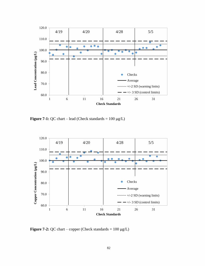
82

Figure 7-1: QC chart – lead (Check standards = 100 µg/L)

Figure 7-2: QC chart – copper (Check standards = 100 µg/L)

60.0

70.0

80.0

90.0

100.0

110.0

120.0

1 6 11 16 21 26 31

Lea

d C

on

cen

tra

tio

n (

µg

/L)

Check Standards

Checks

Average

+/-2 SD (warning linits)

+/- 3 SD (control limits)

60.0

70.0

80.0

90.0

100.0

110.0

120.0

1 6 11 16 21 26 31

Co

pp

er C

on

cen

tra

tio

n (

µg

/L)

Check Standards

Checks

Average

+/-2 SD (warning linits)


4/19 4/20 4/28 5/5

4/19 4/20 4/28 5/5

83

Figure 7-3: QC chart – TOC (Check standards = 2.5 mg/L)

Figure 7-4: QC chart – phosphate (Check standards = 2.0 mg/L)

1.6

1.8

2.0

2.2

2.4

2.6

2.8

3.0

1 6 11 16 21 26

TO

C (

mg

/L)

Check Standards

Check STD

Average

+/- 2 SD (warning limits)


1.0

1.2

1.4

1.6

1.8

2.0

2.2

2.4

1 6 11 16 21

Ph

osp

ha

te (

mg

/L)

Checks

Average

Warning Limits

Control Limits

84

Figure 7-5 : QC chart – chloride (Check standards = 25 mg/L)

Figure 7-6: QC chart – sulfate (Check standards = 30 mg/L)

16.0

18.0

20.0

22.0

24.0

26.0

28.0

30.0

1 6 11 16 21

Ch

lori

de

(mg

/L)

Check Std

Average

Warning Limits

Control Limits

20.0

22.0

24.0

26.0

28.0

30.0

32.0

34.0

1 6 11 16 21

Su

lfa

te (

mg

/L)

Checks

Average

Warning Limits

Control Limits

85

7.2 Raw Data Table 7-1: Total and dissolved lead release for 30-min stagnation periods (part 1)

Experimental

condition Week

Lead release (µg/L)

PVC-Pb: No corrosion

inhibitor

Cu-Pb: No corrosion

inhibitor Cu-Pb: OP Cu-Pb: ZOP Cu-Pb: Sodium silicate

Dissolved Total Dissolved Total Dissolved Total Dissolved Total Dissolved Total

Acclimation

1 5 5 11 13 12 17 9 10 10 14

1 (Tue) 3 9 11 14 14 17 16 16 12 19

3 3 8 10 12 9 10 9 10 11 15

3 (Tue) 6 11 11 15 12 14 15 17 16 17

4 6 6 20 21 17 18 18 19 23 24

4 (Tue) 5 10 11 11 17 17 16 19 16 21

6 0 5 13 13 11 12 12 14 14 16

6 (Tue) 5 6 11 14 13 15 16 19 14 15

Low CMSR

1 8 9 15 15 7 8 16 26 10 10

1 (Tue) 5 7 13 14 7 11 8 16 15 17

3 10 15 22 26 18 19 6 9 11 23

3 (Tue) 4 6 14 26 1 4 1 8 9 18

4 7 7 19 23 1 8 1 6 7 12

5 3 4 21 24 3 3 4 5 15 15

6 4 4 24 25 2 2 2 7 16 18

7 2 4 16 17 2 2 2 3 10 13

8 0 1 16 17 0 0 0 0 7 8

9 6 9 11 19 0 1 0 4 11 18

10 5 6 20 28 1 3 1 4 21 25

11 4 6 19 20 6 7 7 11 19 20

12 19 21 22 21 7 8 6 6 30 31

86

Table 7-1: total and dissolved lead release for 30-min stagnation periods (part 2)

Experimental

condition Week



inhibitor

Cu-Pb: No corrosion



High CSMR-

low

conductivity

1 2 8 13 16 3 4 0 3 17 16

2 5 5 11 12 0 0 0 0 18 20

3 1 1 16 18 0 0 0 0 17 19

4 2 6 16 17 3 2 0 3 18 19

5 2 4 16 18 4 5 0 1 16 17

6 6 8 12 14 4 8 2 4 16 21

High CSMR-

high

conductivity

1 3 4 17 17 1 6 0 4 15 17

2 5 7 16 16 3 4 3 8 9 14

3 7 11 12 20 5 8 0 1 10 11

4 7 9 14 16 3 3 1 3 10 12

5 6 7 13 20 2 2 0 1 9 15

6 5 8 14 17 1 5 -2 1 9 12

7 5 8 17 20 3 3 0 7 11 17

8 6 7 15 24 5 5 0 3 11 13

Table 7-1: total and dissolved lead release for 30-min stagnation periods (part 3)

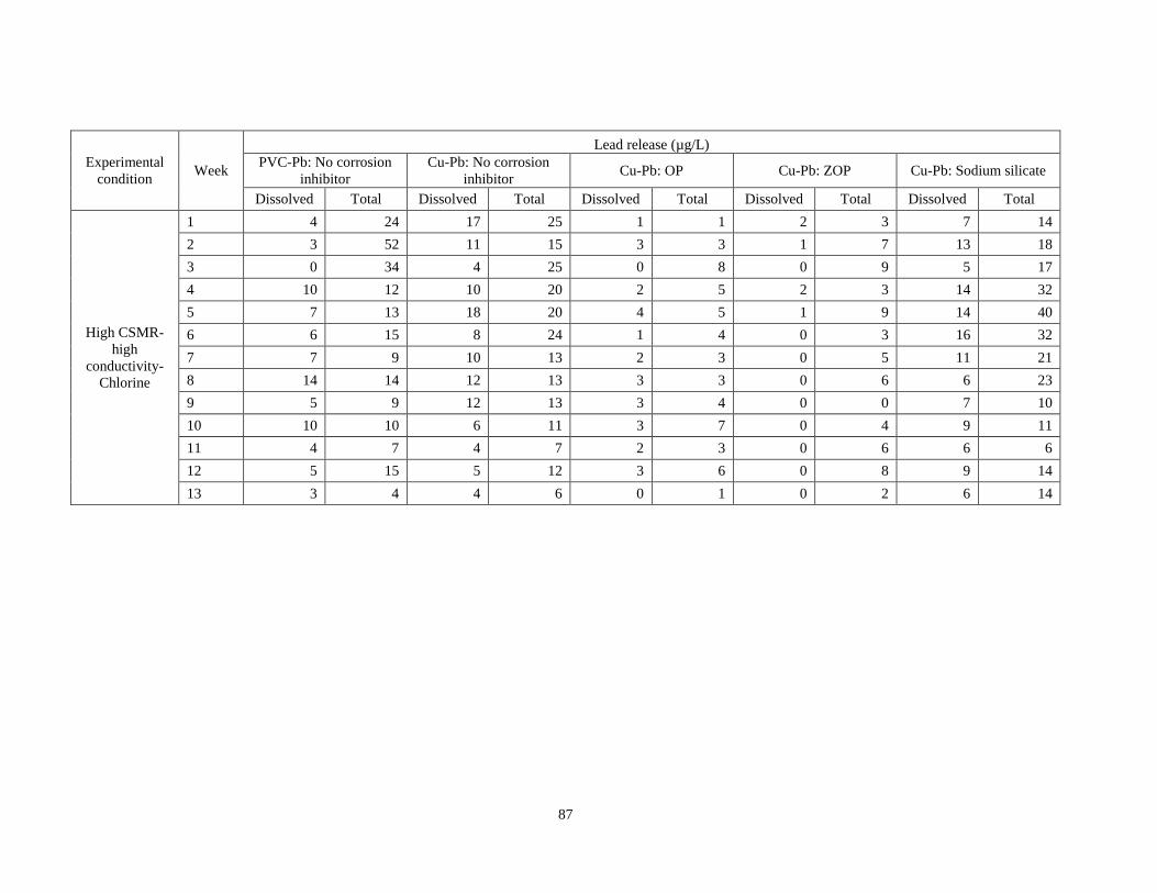
87

Experimental

condition Week



inhibitor

Cu-Pb: No corrosion



High CSMR-

high

conductivity-

Chlorine

1 4 24 17 25 1 1 2 3 7 14

2 3 52 11 15 3 3 1 7 13 18

3 0 34 4 25 0 8 0 9 5 17

4 10 12 10 20 2 5 2 3 14 32

5 7 13 18 20 4 5 1 9 14 40

6 6 15 8 24 1 4 0 3 16 32

7 7 9 10 13 2 3 0 5 11 21

8 14 14 12 13 3 3 0 6 6 23

9 5 9 12 13 3 4 0 0 7 10

10 10 10 6 11 3 7 0 4 9 11

11 4 7 4 7 2 3 0 6 6 6

12 5 15 5 12 3 6 0 8 9 14

13 3 4 4 6 0 1 0 2 6 14

88

Table 7-2: Total and dissolved lead release for 6-h stagnation periods (part 1)

Experimental

condition Week



inhibitor

Cu-Pb: No corrosion



Acclimation

1 14 15 35 34 42 44 30 35 38 43

1 (Tue) 11 22 29 35 36 44 34 36 39 49

3 16 19 32 33 33 39 31 43 39 43

3 (Tue) 11 14 31 32 33 40 33 48 34 42

4 25 28 37 37 48 51 51 52 62 66

4 (Tue) 16 20 25 36 42 45 46 49 46 59

6 16 17 26 32 36 37 36 39 43 47

6 (Tue) 16 16 30 30 36 36 38 40 36 41

Low CMSR

1 22 29 42 47 20 23 33 37 33 34

1 (Tue) 18 21 36 38 13 19 25 21 31 36

3 29 33 63 68 11 20 10 17 40 53

3 (Tue) 19 24 49 55 6 12 8 15 38 43

4 26 29 61 63 9 11 14 20 36 38

5 30 32 59 62 6 8 10 14 49 50

6 29 33 64 68 7 8 10 12 43 50

7 24 25 52 52 3 5 6 8 39 43

8 16 17 55 57 0 0 2 2 51 57

9 18 25 61 62 0 7 0 7 56 57

10 27 28 69 70 8 8 7 8 66 70

11 19 20 45 46 8 12 0 17 52 54

12 23 38 45 50 0 12 0 11 51 64

89

Table 7-2: total and dissolved lead release for 6-h stagnation periods (part 2)

Experimental

condition Week



inhibitor

Cu-Pb: No corrosion



High CSMR-

low

conductivity

1 15 31 43 58 7 17 3 14 52 59

2 20 20 40 40 0 0 0 0 55 55

3 14 15 49 51 3 4 0 5 57 58

4 15 18 50 52 9 10 4 4 53 54

5 18 20 48 50 8 10 2 3 55 55

6 23 24 51 52 7 8 2 5 46 51

High CSMR-

high

conductivity

1 14 20 46 50 7 11 0 7 42 46

2 17 23 41 45 8 9 5 7 39 39

3 16 19 46 49 12 12 3 5 34 36

4 15 18 38 45 6 12 0 3 31 37

5 19 22 36 41 10 10 0 0 35 39

6 14 22 40 48 7 11 1 2 31 35

7 11 20 41 48 9 10 2 5 29 34

8 11 16 34 48 4 4 1 1 25 27

Table 7-2: total and dissolved lead release for 6-h stagnation periods (part 3)

90

Experimental

condition Week



inhibitor

Cu-Pb: No corrosion



High CSMR-

high

conductivity-

Chlorine

1 15 120 47 51 3 8 6 6 32 35

2 13 85 37 59 8 15 2 11 27 41

3 13 45 25 64 0 19 0 15 21 49

4 19 29 29 65 5 16 1 12 23 49

5 22 32 25 50 6 11 4 7 24 58

6 19 28 24 47 9 11 6 6 25 63

7 21 23 23 32 9 11 4 8 22 38

8 23 24 12 20 3 5 3 7 16 49

9 17 21 22 27 5 8 2 4 20 32

10 15 32 16 21 5 8 3 6 16 28

11 10 13 14 18 6 9 5 6 12 28

12 13 26 10 26 3 7 1 9 12 24

13 11 23 21 21 4 6 3 3 13 17

91


Experimental

condition

Week



inhibitor

Cu-Pb: No corrosion



Acclimation

1 62 86 83 97 112 143 133 137 78 102

3 43 65 81 90 117 129 128 155 90 105

4 30 36 96 110 102 118 132 155 111 135

6 48 60 68 85 79 102 101 106 63 70

Low CMSR

1 37 49 103 106 19 20 37 37 62 71

3 38 48 135 155 9 26 14 29 61 79

4 46 47 92 97 9 10 13 13 59 62

5 29 35 91 96 8 10 13 14 68 72

6 29 31 96 103 7 9 5 6 70 73

7 38 42 124 133 10 13 10 11 111 123

8 18 20 139 147 0 7 0 4 122 130

9 32 43 98 124 5 18 7 7 91 124

10 33 34 99 102 10 13 12 14 93 106

11 26 36 71 76 10 19 17 27 92 112

12 21 32 65 76 12 14 7 8 86 99

High CSMR-

low

conductivity

1 36 39 76 75 9 10 1 0 99 103

2 32 35 101 107 5 11 0 7 136 152

3 27 28 107 115 8 10 0 0 96 104

4 23 29 86 96 14 15 2 7 92 112

5 24 29 106 117 13 20 6 8 78 90

6 25 29 98 107 17 18 5 10 86 91


92

Experimental

condition

Week



inhibitor

Cu-Pb: No corrosion



High CSMR-

high

conductivity

1 21 31 111 134 18 26 6 4 66 78

2 32 38 91 105 13 21 6 6 58 70

3 40 55 82 95 15 24 0 6 59 75

4 36 46 90 99 18 27 3 11 62 67

5 37 50 96 115 12 27 0 6 51 61

6 34 45 79 84 20 22 1 4 53 60

7 36 42 84 97 11 14 1 1 37 40

8 25 31 86 88 16 17 5 5 48 50

High CSMR-

high

conductivity-

Chlorine

1 34 138 79 91 25 28 9 10 47 59

2 48 137 73 102 24 38 8 16 50 63

3 54 74 57 73 36 51 8 17 59 79

4 58 93 54 75 39 54 8 8 49 74

5 36 49 42 45 35 46 5 7 44 128

6 38 42 56 61 44 54 0 10 33 60

7 41 52 26 27 26 34 4 5 31 49

8 53 58 38 45 22 30 3 6 30 32

9 38 42 34 38 12 17 0 6 37 41

10 39 43 44 51 15 17 3 5 32 34

11 22 25 29 31 10 11 5 4 30 35

12 29 32 24 26 14 18 3 3 24 29

13 23 28 31 31 14 19 4 6 41 42

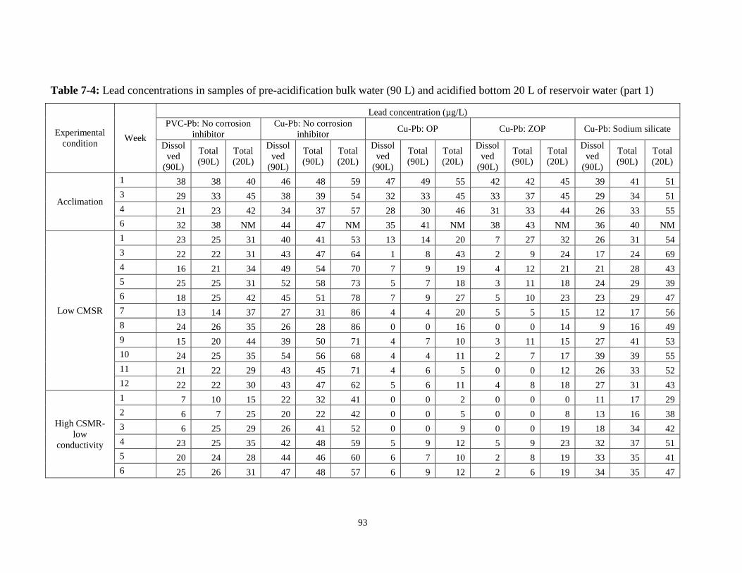
93

Table 7-4: Lead concentrations in samples of pre-acidification bulk water (90 L) and acidified bottom 20 L of reservoir water (part 1)

Experimental

condition Week

Lead concentration (µg/L)


inhibitor

Cu-Pb: No corrosion


Dissol

ved

(90L)

Total

(90L)

Total

(20L)

Dissol

ved

(90L)

Total

(90L)

Total

(20L)

Dissol

ved

(90L)

Total

(90L)

Total

(20L)

Dissol

ved

(90L)

Total

(90L)

Total

(20L)

Dissol

ved

(90L)

Total

(90L)

Total

(20L)

Acclimation

1 38 38 40 46 48 59 47 49 55 42 42 45 39 41 51

3 29 33 45 38 39 54 32 33 45 33 37 45 29 34 51

4 21 23 42 34 37 57 28 30 46 31 33 44 26 33 55

6 32 38 NM 44 47 NM 35 41 NM 38 43 NM 36 40 NM

Low CMSR

1 23 25 31 40 41 53 13 14 20 7 27 32 26 31 54

3 22 22 31 43 47 64 1 8 43 2 9 24 17 24 69

4 16 21 34 49 54 70 7 9 19 4 12 21 21 28 43

5 25 25 31 52 58 73 5 7 18 3 11 18 24 29 39

6 18 25 42 45 51 78 7 9 27 5 10 23 23 29 47

7 13 14 37 27 31 86 4 4 20 5 5 15 12 17 56

8 24 26 35 26 28 86 0 0 16 0 0 14 9 16 49

9 15 20 44 39 50 71 4 7 10 3 11 15 27 41 53

10 24 25 35 54 56 68 4 4 11 2 7 17 39 39 55

11 21 22 29 43 45 71 4 6 5 0 0 12 26 33 52

12 22 22 30 43 47 62 5 6 11 4 8 18 27 31 43

High CSMR-

low

conductivity

1 7 10 15 22 32 41 0 0 2 0 0 0 11 17 29

2 6 7 25 20 22 42 0 0 5 0 0 8 13 16 38

3 6 25 29 26 41 52 0 0 9 0 0 19 18 34 42

4 23 25 35 42 48 59 5 9 12 5 9 23 32 37 51

5 20 24 28 44 46 60 6 7 10 2 8 19 33 35 41

6 25 26 31 47 48 57 6 9 12 2 6 19 34 35 47

94

Table 7-4: Lead concentrations in samples of pre-acidification bulk water (90 L) and acidified bottom 20 L of reservoir water (part 2)

Experimental

condition Week

Lead concentration (µg/L)


inhibitor

Cu-Pb: No corrosion


Dissol

ved

(90L)

Total

(90L)

Total

(20L)

Dissol

ved

(90L)

Total

(90L)

Total

(20L)

Dissol

ved

(90L)

Total

(90L)

Total

(20L)

Dissol

ved

(90L)

Total

(90L)

Total

(20L)

Dissol

ved

(90L)

Total

(90L)

Total

(20L)

High CSMR-

high

conductivity

1 24 26 31 46 54 60 7 12 14 2 7 18 36 36 46

2 17 19 44 26 29 88 2 3 16 2 5 17 20 22 70

3 16 18 39 35 36 55 2 4 6 1 2 14 27 26 46

4 18 21 36 31 33 53 4 7 7 3 3 14 26 26 51

5 20 20 33 36 39 57 2 3 11 0 5 12 27 31 41

6 19 20 32 42 45 61 4 4 11 0 1 19 27 29 40

7 21 22 28 39 42 56 8 8 14 4 7 22 28 28 48

8 18 20 30 33 34 45 6 6 10 0 4 21 22 24 32

High CSMR-

high

conductivity-

Chlorine

1 21 24 37 37 48 76 7 10 24 9 20 55 35 36 63

2 17 23 36 37 46 77 3 8 26 4 11 32 29 36 68

3 20 27 52 45 52 88 10 15 34 5 12 27 34 45 83

4 22 25 50 43 47 73 5 11 23 3 16 30 40 42 114

5 26 27 38 32 40 58 6 8 13 0 12 29 38 41 170

6 22 29 39 35 41 59 3 9 18 1 7 26 33 39 123

7 22 25 35 29 36 49 8 9 15 3 8 21 30 32 62

8 20 21 35 32 33 48 9 9 15 3 7 19 31 33 60

9 21 21 32 25 27 35 6 7 14 2 8 16 21 25 42

10 15 16 25 22 22 39 1 4 9 1 4 11 23 23 32

11 16 18 34 18 19 31 2 4 11 0 3 9 13 15 22

12 17 21 29 20 25 36 6 10 13 2 10 10 17 19 37

13 18 22 29 23 24 32 5 8 10 2 7 11 21 22 27

NM represents not measured. In acclimation Week 4, reservoir water was not changed until the end of Week 5 because water was not collected for the following

week.

95

Dissolved (90L) and Total (90L) samples were collected before the weekly reservoir acidification and represent the lead concentrations in the bulk water. Total (20L)

samples were collected after the reservoir acidification of the bottom 20 L of reservoir water and represent total lead concentrations in the reservoir including the bulk

water and particulates at the bottom of the reservoir.

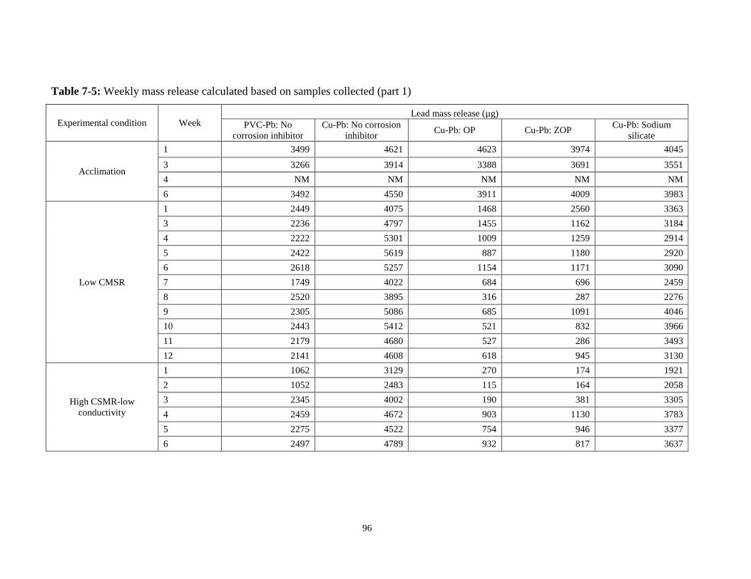
96

Table 7-5: Weekly mass release calculated based on samples collected (part 1)

Experimental condition Week Lead mass release (µg)

PVC-Pb: No

corrosion inhibitor

Cu-Pb: No corrosion

inhibitor Cu-Pb: OP Cu-Pb: ZOP

Cu-Pb: Sodium

silicate

Acclimation

1 3499 4621 4623 3974 4045

3 3266 3914 3388 3691 3551

4 NM NM NM NM NM

6 3492 4550 3911 4009 3983

Low CMSR

1 2449 4075 1468 2560 3363

3 2236 4797 1455 1162 3184

4 2222 5301 1009 1259 2914

5 2422 5619 887 1180 2920

6 2618 5257 1154 1171 3090

7 1749 4022 684 696 2459

8 2520 3895 316 287 2276

9 2305 5086 685 1091 4046

10 2443 5412 521 832 3966

11 2179 4680 527 286 3493

12 2141 4608 618 945 3130

High CSMR-low

conductivity

1 1062 3129 270 174 1921

2 1052 2483 115 164 2058

3 2345 4002 190 381 3305

4 2459 4672 903 1130 3783

5 2275 4522 754 946 3377

6 2497 4789 932 817 3637

97

Table 7-5: Weekly mass release calculated based on samples collected (part 2)

Experimental condition Week Lead mass release (µg)

PVC-Pb: No

corrosion inhibitor

Cu-Pb: No corrosion


Cu-Pb: Sodium

silicate

High CSMR-high

conductivity

1 2507 5264 1191 901 3661

2 2279 4063 555 719 3161

3 2101 3715 439 466 2862

4 2231 3484 650 523 2933

5 2093 3961 483 588 3060

6 2099 4443 501 485 2876

7 2128 4189 859 920 2993

8 2042 3377 629 723 2375

High CSMR-high

conductivity-Chlorine

1 2642 4979 1195 2483 3847

2 2508 4844 1152 1464 3968

3 3028 5452 1765 1388 4879

4 2843 4804 1231 1711 5288

5 2728 3991 866 1401 6380

6 2860 4100 1042 999 5288

7 2477 3520 930 991 3555

8 2194 3290 948 900 3516

9 2164 2595 753 851 2660

10 1690 2375 496 538 2262

11 1959 2031 532 434 1513

12 2071 2591 952 919 2097

13 2130 2363 786 737 2087

98

Table 7-6: Total and dissolved copper release for 30-min stagnation periods (part 1)

Experimental

condition Week

Copper release (µg/L)


inhibitor

Cu-Pb: No corrosion



Acclimation

1 0 0 36 36 34 30 35 27 41 39

1 (Tue) 0 0 30 38 32 35 37 28 37 39

3 0 0 30 31 28 27 29 27 33 33

3 (Tue) -2 0 24 33 25 29 24 29 27 29

4 0 1 36 34 34 33 33 32 36 37

4 (Tue) 0 0 34 37 28 28 31 29 32 36

6 0 0 24 39 23 37 24 37 30 46

6 (Tue) 0 0 34 29 29 27 31 25 35 31

Low CMSR

1 0 0 26 17 6 6 9 6 22 20

1 (Tue) 0 0 18 19 -2 1 1 1 18 18

3 0 0 14 18 -7 -10 4 5 13 19

3 (Tue) 0 -1 9 9 0 -2 1 0 11 10

4 0 -1 18 18 6 4 4 3 19 18

5 2 0 24 25 6 5 5 5 27 29

6 0 1 21 21 4 3 3 3 22 22

7 0 0 21 20 11 10 6 4 16 18

8 0 0 20 16 4 3 2 2 14 12

9 0 0 16 25 5 11 1 5 26 36

10 6 0 40 23 29 10 17 5 40 23

11 0 1 21 8 3 -3 4 -6 21 9

12 0 0 22 24 9 10 2 3 26 27


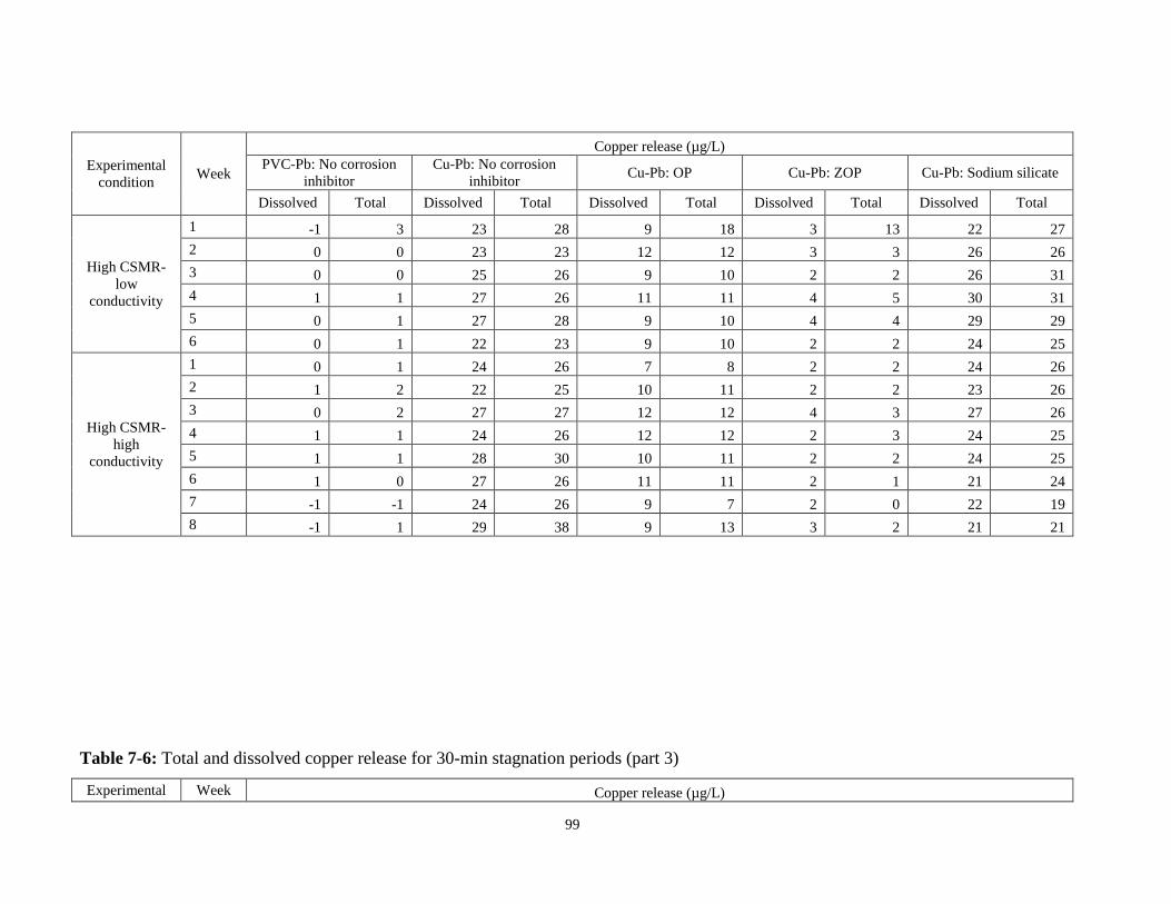
99

Experimental

condition Week



inhibitor

Cu-Pb: No corrosion



High CSMR-

low

conductivity

1 -1 3 23 28 9 18 3 13 22 27

2 0 0 23 23 12 12 3 3 26 26

3 0 0 25 26 9 10 2 2 26 31

4 1 1 27 26 11 11 4 5 30 31

5 0 1 27 28 9 10 4 4 29 29

6 0 1 22 23 9 10 2 2 24 25

High CSMR-

high

conductivity

1 0 1 24 26 7 8 2 2 24 26

2 1 2 22 25 10 11 2 2 23 26

3 0 2 27 27 12 12 4 3 27 26

4 1 1 24 26 12 12 2 3 24 25

5 1 1 28 30 10 11 2 2 24 25

6 1 0 27 26 11 11 2 1 21 24

7 -1 -1 24 26 9 7 2 0 22 19

8 -1 1 29 38 9 13 3 2 21 21


Experimental Week Copper release (µg/L)

100

condition PVC-Pb: No corrosion

inhibitor

Cu-Pb: No corrosion



High CSMR-

high

conductivity-

Chlorine

1 -1 0 62 65 21 24 14 14 38 47

2 1 1 34 36 15 19 8 7 30 35

3 3 2 37 52 12 21 7 7 28 39

4 1 1 32 41 12 14 7 5 21 26

5 2 2 43 53 14 14 4 6 37 50

6 2 1 41 50 15 12 4 4 32 36

7 0 0 32 41 10 11 3 3 36 39

8 0 0 44 45 11 13 2 4 30 34

9 0 1 31 32 9 11 3 2 28 31

10 1 1 29 36 9 12 1 3 32 39

11 1 1 23 26 8 9 1 2 22 23

12 3 1 24 45 12 14 2 3 5 34

13 0 1 30 32 8 9 2 -1 24 31

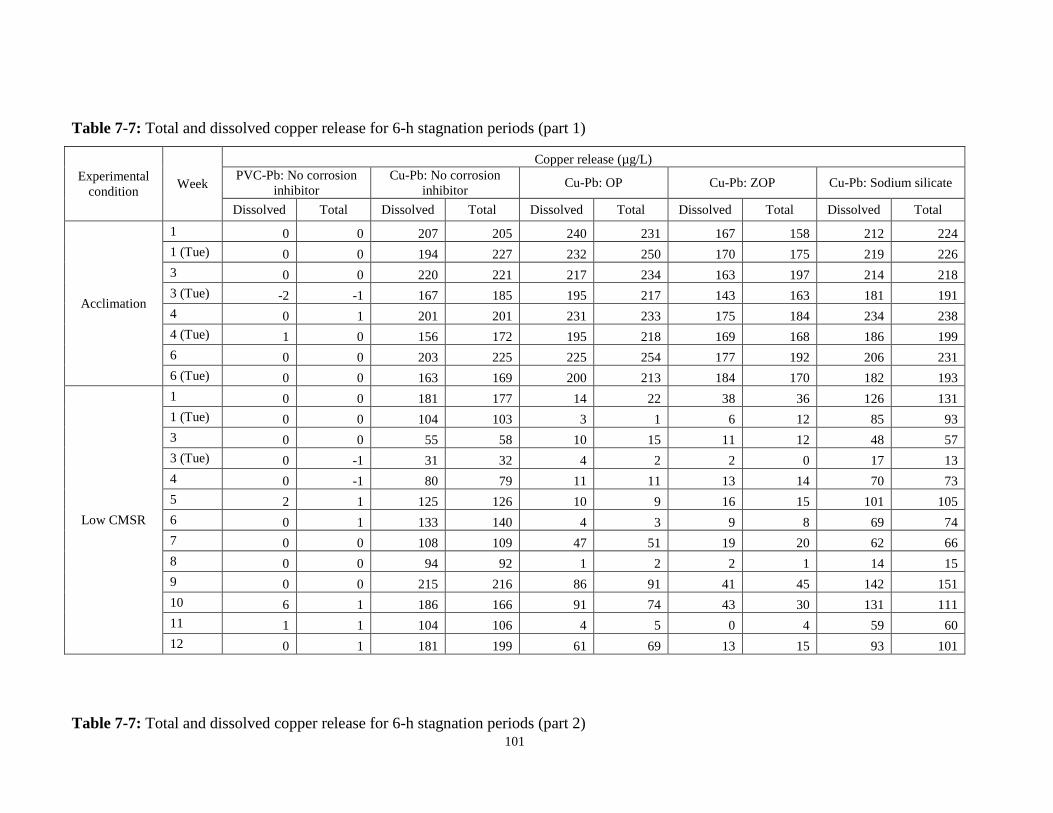
101

Table 7-7: Total and dissolved copper release for 6-h stagnation periods (part 1)

Experimental

condition Week



inhibitor

Cu-Pb: No corrosion



Acclimation

1 0 0 207 205 240 231 167 158 212 224

1 (Tue) 0 0 194 227 232 250 170 175 219 226

3 0 0 220 221 217 234 163 197 214 218

3 (Tue) -2 -1 167 185 195 217 143 163 181 191

4 0 1 201 201 231 233 175 184 234 238

4 (Tue) 1 0 156 172 195 218 169 168 186 199

6 0 0 203 225 225 254 177 192 206 231

6 (Tue) 0 0 163 169 200 213 184 170 182 193

Low CMSR

1 0 0 181 177 14 22 38 36 126 131

1 (Tue) 0 0 104 103 3 1 6 12 85 93

3 0 0 55 58 10 15 11 12 48 57

3 (Tue) 0 -1 31 32 4 2 2 0 17 13

4 0 -1 80 79 11 11 13 14 70 73

5 2 1 125 126 10 9 16 15 101 105

6 0 1 133 140 4 3 9 8 69 74

7 0 0 108 109 47 51 19 20 62 66

8 0 0 94 92 1 2 2 1 14 15

9 0 0 215 216 86 91 41 45 142 151

10 6 1 186 166 91 74 43 30 131 111

11 1 1 104 106 4 5 0 4 59 60

12 0 1 181 199 61 69 13 15 93 101


102

Experimental

condition Week



inhibitor

Cu-Pb: No corrosion



High CSMR-

low

conductivity

1 1 2 170 177 65 72 21 23 100 104

2 0 0 167 167 69 70 17 17 100 102

3 1 2 133 136 39 40 13 13 95 104

4 2 2 190 194 74 76 20 20 117 123

5 -1 -1 191 194 72 79 20 22 125 129

6 0 0 174 182 53 57 12 13 80 86

High CSMR-

high

conductivity

1 -1 0 133 141 32 34 6 7 78 78

2 1 2 104 119 40 45 5 6 86 98

3 1 1 161 168 65 69 12 12 105 108

4 0 0 168 177 60 64 8 9 96 102

5 2 2 138 142 47 50 7 7 85 90

6 0 0 198 202 62 65 11 11 90 96

7 -1 -2 165 172 43 41 7 6 91 92

8 5 7 165 189 56 63 15 12 70 75


Experimental Week Copper release (µg/L)

103

condition PVC-Pb: No corrosion

inhibitor

Cu-Pb: No corrosion



High CSMR-

high

conductivity-

Chlorine

1 1 3 209 231 99 108 45 46 155 160

2 2 2 139 160 87 98 40 42 112 125

3 2 3 141 171 65 81 37 39 85 104

4 3 2 113 137 48 56 27 28 53 78

5 2 2 89 121 52 62 20 23 78 92

6 2 2 103 125 40 41 16 16 76 81

7 1 0 94 109 37 40 15 16 80 97

8 1 1 71 77 44 49 10 11 71 80

9 1 1 85 87 28 29 8 9 79 83

10 2 2 83 98 29 35 6 8 78 88

11 1 1 68 78 26 26 6 6 64 70

12 1 3 69 102 23 34 4 6 72 99

13 0 0 89 95 26 28 5 4 68 72

104


Experimental

condition

Week Copper release (µg/L)


inhibitor

Cu-Pb: No corrosion

inhibitor

Cu-Pb: OP Cu-Pb: ZOP Cu-Pb: Sodium silicate


Acclimation 1 0 0 19 27 24 30 12 15 -1 -2

3 3 1 5 4 19 19 12 14 5 6

4 0 0 15 11 8 6 7 5 -1 -2

6 -2 1 173 183 33 39 1 -1 276 267

Low CMSR 1 -2 0 -4 -4 26 26 32 27 32 39

3 -0 -2 5 4 43 43 30 27 1 -0

4 -0 -4 7 -1 27 20 23 16 0 -5

5 -1 7 -4 2 27 34 20 26 -3 2

6 3 5 -9 -4 15 24 8 16 -7 2

7 0 0 -1 -2 12 11 10 5 -4 -10

8 0 0 -7 -8 7 8 12 11 0 -1

9 0 0 -9 -9 6 11 10 17 -6 -6

10 -0 -0 -13 -16 9 7 20 17 -11 -11

11 0 0 -12 -18 13 -4 18 10 -5 -13

12 -1 -0 -20 -20 1 1 8 9 -13 -13

High CSMR-

low

conductivity

1 0 2 5 5 4 7 12 12 -7 -8

2 0 0 -8 -7 8 8 18 20 -2 -2

3 -0 -1 -10 -14 5 4 12 9 -10 -15

4 1 2 -13 -14 5 6 10 12 -9 -9

5 0 0 -15 -15 6 7 9 11 -14 -13

6 0 1 -11 -12 8 8 11 11 -4 -6


105

Experimental

condition

Week Copper release (µg/L)


inhibitor

Cu-Pb: No corrosion

inhibitor

Cu-Pb: OP Cu-Pb: ZOP Cu-Pb: Sodium silicate


High CSMR-

high

conductivity

1 2 2 -12 -11 6 6 5 5 -11 -12

2 -1 -0 -4 -9 6 6 8 10 -10 -13

3 -1 -2 -8 -10 12 8 5 3 -16 -18

4 0 1 -8 -7 8 8 4 5 -14 -15

5 0 1 -12 -8 2 4 7 8 -15 -13

6 1 1 -13 -12 7 8 3 3 -14 -16

7 1 1 -14 -11 2 2 4 3 1 1

8 2 5 1 -0 8 12 10 12 -14 -12

High CSMR-

high

conductivity-

Chlorine

1 5 9 160 177 250 266 106 120 34 47

2 8 11 382 440 274 314 122 139 145 176

3 7 9 236 260 284 323 76 85 156 170

4 9 10 226 251 218 232 51 57 107 129

5 7 7 122 137 126 154 34 39 76 113

6 5 1 161 147 173 179 64 65 82

7 3 4 75 86 117 128 20 20 71 81

8 4 5 96 102 133 146 40 45 78 84

9 4 4 104 121 103 112 46 51 206 223

10 3 4 116 110 105 108 39 39 86 92

11 3 3 80 79 60 61 20 20 169 168

12 2 3 92 94 104 109 23 26 244 268

13 2 2 86 98 99 104 18 19 145 150

106

Table 7-9: Copper concentrations in samples of pre-acidification bulk water (90 L) and acidified bottom 20 L of reservoir water (part 1)

Experimental

condition Week

Copper concentration (µg/L)


inhibitor

Cu-Pb: No corrosion


Dissol

ved

(90L)

Total

(90L)

Total

(20L)

Dissol

ved

(90L)

Total

(90L)

Total

(20L)

Dissol

ved

(90L)

Total

(90L)

Total

(20L)

Dissol

ved

(90L)

Total

(90L)

Total

(20L)

Dissol

ved

(90L)

Total

(90L)

Total

(20L)

Acclimation

1 0 0 0 43 49 55 42 50 53 38 43 46 40 45 56

3 2 3 4 47 53 61 47 54 59 42 50 53 46 53 70

4 0 0 NM 36 43 NM 33 39 NM 29 36 NM 33 39 NM

6 6 5 6 60 64 70 55 58 63 54 57 60 58 61 75

Low CMSR

1 6 5 8 42 46 50 20 26 32 13 22 27 32 35 50

3 0 4 5 19 23 37 6 12 24 5 10 18 17 25 43

4 3 7 9 31 40 52 11 18 27 7 15 21 23 33 42

5 9 1 2 48 46 57 17 11 22 13 8 14 35 31 41

6 0 0 0 36 34 46 13 8 20 10 5 8 25 21 29

7 0 0 0 23 27 53 5 8 26 1 7 13 14 23 39

8 0 0 2 31 34 60 7 10 27 1 3 12 14 17 30

9 0 3 9 30 43 56 0 18 30 0 12 19 18 36 47

10 3 4 4 51 55 63 17 19 30 8 12 16 38 41 52

11 0 2 3 37 43 59 9 26 28 0 9 14 23 33 43

12 2 2 2 42 46 57 15 17 25 6 7 12 29 32 39

High CSMR-

low

conductivity

1 11 10 10 43 44 57 28 28 35 15 16 18 34 37 42

2 11 11 3 46 49 51 26 27 28 15 16 11 36 39 39

3 2 2 4 40 46 57 14 16 22 5 9 12 27 33 42

4 4 5 5 45 49 58 19 19 24 10 11 14 34 37 47

5 4 4 5 46 50 54 19 20 25 9 10 12 32 35 39

6 4 4 5 41 44 51 17 19 24 8 9 11 29 33 39

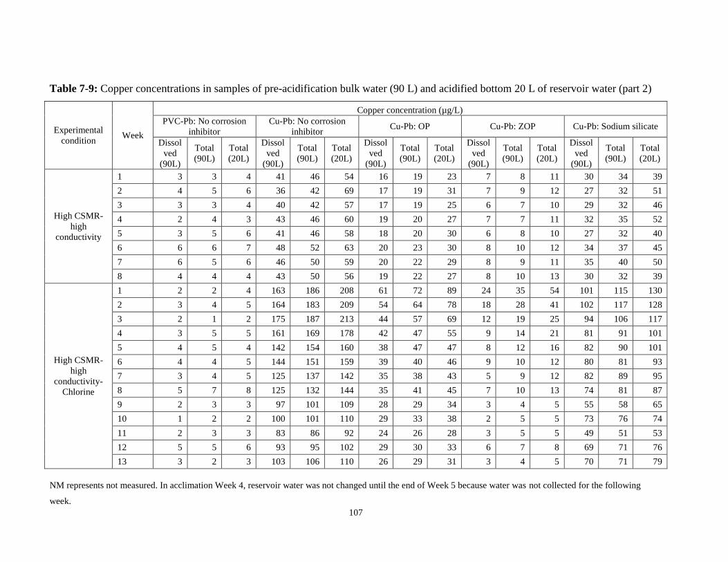
107

Table 7-9: Copper concentrations in samples of pre-acidification bulk water (90 L) and acidified bottom 20 L of reservoir water (part 2)

Experimental

condition Week

Copper concentration (µg/L)


inhibitor

Cu-Pb: No corrosion


Dissol

ved

(90L)

Total

(90L)

Total

(20L)

Dissol

ved

(90L)

Total

(90L)

Total

(20L)

Dissol

ved

(90L)

Total

(90L)

Total

(20L)

Dissol

ved

(90L)

Total

(90L)

Total

(20L)

Dissol

ved

(90L)

Total

(90L)

Total

(20L)

High CSMR-

high

conductivity

1 3 3 4 41 46 54 16 19 23 7 8 11 30 34 39

2 4 5 6 36 42 69 17 19 31 7 9 12 27 32 51

3 3 3 4 40 42 57 17 19 25 6 7 10 29 32 46

4 2 4 3 43 46 60 19 20 27 7 7 11 32 35 52

5 3 5 6 41 46 58 18 20 30 6 8 10 27 32 40

6 6 6 7 48 52 63 20 23 30 8 10 12 34 37 45

7 6 5 6 46 50 59 20 22 29 8 9 11 35 40 50

8 4 4 4 43 50 56 19 22 27 8 10 13 30 32 39

High CSMR-

high

conductivity-

Chlorine

1 2 2 4 163 186 208 61 72 89 24 35 54 101 115 130

2 3 4 5 164 183 209 54 64 78 18 28 41 102 117 128

3 2 1 2 175 187 213 44 57 69 12 19 25 94 106 117

4 3 5 5 161 169 178 42 47 55 9 14 21 81 91 101

5 4 5 4 142 154 160 38 47 47 8 12 16 82 90 101

6 4 4 5 144 151 159 39 40 46 9 10 12 80 81 93

7 3 4 5 125 137 142 35 38 43 5 9 12 82 89 95

8 5 7 8 125 132 144 35 41 45 7 10 13 74 81 87

9 2 3 3 97 101 109 28 29 34 3 4 5 55 58 65

10 1 2 2 100 101 110 29 33 38 2 5 5 73 76 74

11 2 3 3 83 86 92 24 26 28 3 5 5 49 51 53

12 5 5 6 93 95 102 29 30 33 6 7 8 69 71 76

13 3 2 3 103 106 110 26 29 31 3 4 5 70 71 79

NM represents not measured. In acclimation Week 4, reservoir water was not changed until the end of Week 5 because water was not collected for the following

week.

108

Dissolved (90L) and Total (90L) samples were collected before the weekly reservoir acidification and represent the copper concentrations in the bulk water. Total

(20L) samples were collected after the reservoir acidification of the bottom 20 L of reservoir water and represent total copper concentrations in the reservoir including

the bulk water and particulates at the bottom of the reservoir.

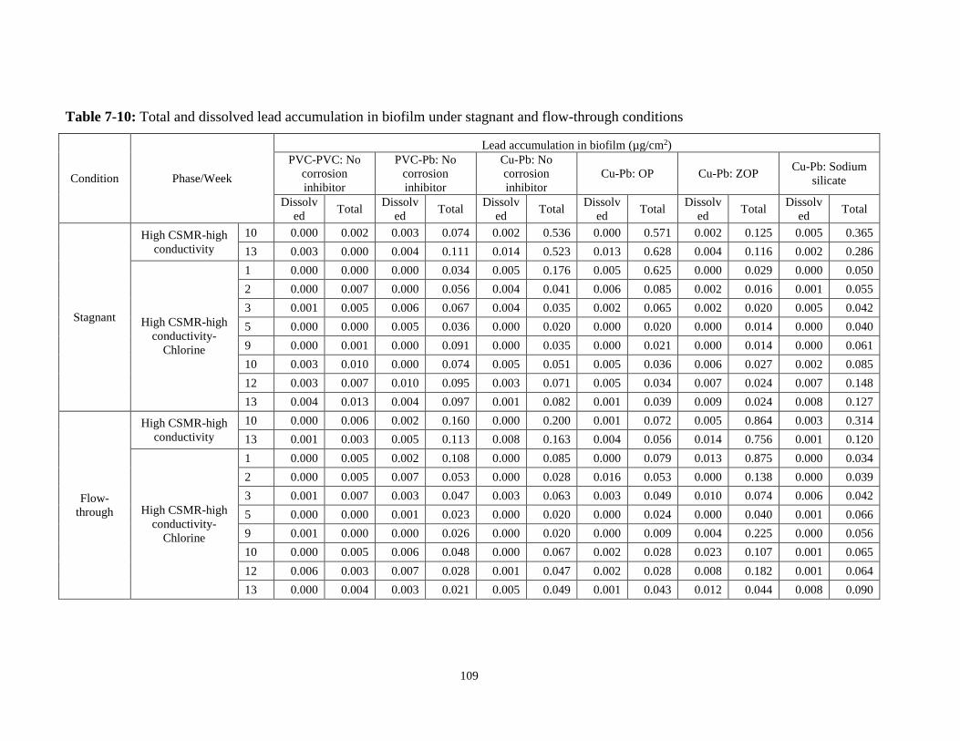
109

Table 7-10: Total and dissolved lead accumulation in biofilm under stagnant and flow-through conditions

Condition Phase/Week

Lead accumulation in biofilm (µg/cm2)

PVC-PVC: No

corrosion

inhibitor

PVC-Pb: No

corrosion

inhibitor

Cu-Pb: No

corrosion

inhibitor

Cu-Pb: OP Cu-Pb: ZOP Cu-Pb: Sodium

silicate

Dissolv

ed Total

Dissolv

ed Total

Dissolv

ed Total

Dissolv

ed Total

Dissolv

ed Total

Dissolv

ed Total

Stagnant

High CSMR-high

conductivity

10 0.000 0.002 0.003 0.074 0.002 0.536 0.000 0.571 0.002 0.125 0.005 0.365

13 0.003 0.000 0.004 0.111 0.014 0.523 0.013 0.628 0.004 0.116 0.002 0.286

High CSMR-high

conductivity-

Chlorine

1 0.000 0.000 0.000 0.034 0.005 0.176 0.005 0.625 0.000 0.029 0.000 0.050

2 0.000 0.007 0.000 0.056 0.004 0.041 0.006 0.085 0.002 0.016 0.001 0.055

3 0.001 0.005 0.006 0.067 0.004 0.035 0.002 0.065 0.002 0.020 0.005 0.042

5 0.000 0.000 0.005 0.036 0.000 0.020 0.000 0.020 0.000 0.014 0.000 0.040

9 0.000 0.001 0.000 0.091 0.000 0.035 0.000 0.021 0.000 0.014 0.000 0.061

10 0.003 0.010 0.000 0.074 0.005 0.051 0.005 0.036 0.006 0.027 0.002 0.085

12 0.003 0.007 0.010 0.095 0.003 0.071 0.005 0.034 0.007 0.024 0.007 0.148

13 0.004 0.013 0.004 0.097 0.001 0.082 0.001 0.039 0.009 0.024 0.008 0.127

Flow-

through

High CSMR-high

conductivity

10 0.000 0.006 0.002 0.160 0.000 0.200 0.001 0.072 0.005 0.864 0.003 0.314

13 0.001 0.003 0.005 0.113 0.008 0.163 0.004 0.056 0.014 0.756 0.001 0.120

High CSMR-high

conductivity-

Chlorine

1 0.000 0.005 0.002 0.108 0.000 0.085 0.000 0.079 0.013 0.875 0.000 0.034

2 0.000 0.005 0.007 0.053 0.000 0.028 0.016 0.053 0.000 0.138 0.000 0.039

3 0.001 0.007 0.003 0.047 0.003 0.063 0.003 0.049 0.010 0.074 0.006 0.042

5 0.000 0.000 0.001 0.023 0.000 0.020 0.000 0.024 0.000 0.040 0.001 0.066

9 0.001 0.000 0.000 0.026 0.000 0.020 0.000 0.009 0.004 0.225 0.000 0.056

10 0.000 0.005 0.006 0.048 0.000 0.067 0.002 0.028 0.023 0.107 0.001 0.065

12 0.006 0.003 0.007 0.028 0.001 0.047 0.002 0.028 0.008 0.182 0.001 0.064

13 0.000 0.004 0.003 0.021 0.005 0.049 0.001 0.043 0.012 0.044 0.008 0.090

110

Table 7-11: Total and dissolved copper accumulation in biofilm under stagnant and flow-through conditions

Condition Phase/Week

Copper accumulation in biofilm (µg/cm2)

PVC-PVC: No

corrosion

inhibitor

PVC-Pb: No

corrosion

inhibitor

Cu-Pb: No

corrosion

inhibitor

Cu-Pb: OP

Cu-Pb: ZOP

Cu-Pb: Sodium

silicate

Dissolv

ed Total

Dissolv

ed Total

Dissolv

ed Total

Dissolv

ed Total

Dissolv

ed Total

Dissolv

ed Total

Stagnant

High CSMR-high

conductivity

10 0.004 0.006 0.002 0.028 0.007 0.533 0.007 0.800 0.004 0.084 0.010 0.339

13 0.006 0.031 0.006 0.014 0.046 0.620 0.053 0.834 0.009 0.061 0.021 0.316

High CSMR-high

conductivity-

Chlorine

1 0.007 0.016 0.007 0.016 0.046 0.371 0.032 0.777 0.007 0.023 0.016 0.093

2 0.007 0.005 0.007 0.004 0.007 0.056 0.007 0.071 0.013 0.018 0.012 0.033

3 0.001 0.007 0.001 0.006 0.004 0.029 0.002 0.027 0.001 0.011 0.002 0.025

5 0.002 0.005 0.001 0.005 0.003 0.023 0.003 0.012 0.003 0.010 0.003 0.031

9 0.000 0.003 0.000 0.004 0.002 0.024 0.001 0.014 0.001 0.007 0.004 0.029

10 0.004 0.008 0.004 0.010 0.004 0.031 0.005 0.014 0.004 0.013 0.005 0.032

12 0.004 0.009 0.006 0.010 0.006 0.037 0.006 0.015 0.006 0.012 0.005 0.067

13 0.006 0.011 0.006 0.012 0.006 0.040 0.006 0.017 0.007 0.013 0.007 0.043

Flow-

through

High CSMR-high

conductivity

10 0.000 0.013 0.002 0.031 0.005 0.181 0.006 0.181 0.013 0.477 0.007 0.281

13 0.006 0.037 0.006 0.037 0.016 0.257 0.013 0.110 0.027 0.359 0.010 0.435

High CSMR-high

conductivity-

Chlorine

1 0.007 0.017 0.008 0.019 0.018 0.162 0.015 0.142 0.022 0.387 0.016 0.070

2 0.013 0.008 0.018 0.007 0.007 0.032 0.018 0.062 0.009 0.066 0.012 0.037

3 0.001 0.005 0.002 0.008 0.004 0.047 0.009 0.065 0.004 0.032 0.005 0.035

5 0.002 0.008 0.002 0.005 0.003 0.032 0.005 0.028 0.004 0.018 0.006 0.032

9 0.001 0.005 0.002 0.005 0.003 0.032 0.002 0.014 0.004 0.044 0.005 0.045

10 0.005 0.008 0.004 0.008 0.008 0.058 0.005 0.015 0.008 0.041 0.008 0.039

12 0.006 0.009 0.005 0.012 0.007 0.050 0.006 0.020 0.006 0.044 0.009 0.041

13 0.005 0.008 0.005 0.010 0.007 0.049 0.007 0.027 0.005 0.016 0.012 0.060

111

Table 7-12: ATP accumulation under stagnant (Stag) and flow-through (Flow) conditions

Experimental phases/

Week

ATP (µg/cm2)

PVC-PVC: No

corrosion inhibitor

PVC-Pb: No

corrosion inhibitor

Cu-Pb: No

corrosion inhibitor Cu-Pb: OP Cu-Pb: ZOP

Cu-Pb: Sodium

silicate

Stag Flow Stag Flow Stag Flow Stag Flow Stag Flow Stag Flow

Low CSMR

0 3.66 2.48 11.90 6.45 7.09 2.43 12.15 5.93 5.43 2.05 9.05 2.37

2 2.75 1.59 20.93 5.59 47.26 3.68 15.58 4.92 8.93 5.24 26.12 3.81

4 4.43 3.29 41.83 5.69 22.47 5.00 64.08 16.16 47.52 36.57 15.82 7.78

6 5.45 4.71 72.02 7.45 40.02 12.58 40.83 21.43 33.32 44.26 9.02 9.05

8 9.69 9.98 204.94 19.98 82.76 14.04 121.74 40.78 38.20 96.68 14.40 29.46

10 6.06 4.86 73.77 7.86 53.53 5.59 60.80 25.58 24.54 63.62 21.69 18.08

12 7.62 6.63 46.26 13.41 53.42 6.05 69.18 18.29 27.28 67.10 30.73 13.86

High CSMR-low

conductivity

2 14.73 8.52 45.85 19.97 84.64 8.28 151.77 30.72 34.66 78.86 52.94 26.58

4 2.51 11.84 44.50 26.02 46.46 16.82 232.35 30.79 20.72 68.12 59.27 35.35

High CSMR-high

conductivity

4 9.92 16.57 17.79 35.36 153.51 34.45 376.05 86.31 12.00 136.11 86.62 82.21

8 5.34 16.54 25.13 14.46 150.41 24.11 246.39 34.61 28.98 186.69 157.48 14.95

High CSMR-high

conductivity-Cl2

1 0.02 5.53 0.03 2.71 13.86 3.05 127.27 9.83 0.83 13.34 1.23 7.14

2 0.01 0.02 0.02 0.54 0.01 1.34 1.00 0.31 0.03 1.31 0.03 2.97

3 0.06 0.87 0.01 0.04 0.03 2.86 0.01 1.53 0.16 0.12 0.06 1.86

5 0.01 0.45 0.07 0.01 0.02 0.16 0.11 1.22 0.01 0.01 0.01 0.61

9 0.00 0.31 0.00 0.28 0.00 0.01 0.00 0.40 0.00 0.20 0.00 0.03

10 0.00 0.32 0.00 0.31 0.00 0.00 0.00 0.03 0.00 0.39 0.01 0.01

12 0.00 0.12 0.00 0.09 0.00 0.02 0.00 0.06 0.01 0.14 0.00 0.03

13 0.00 0.10 0.01 0.09 0.00 0.00 0.00 0.10 0.00 0.06 0.00 0.01

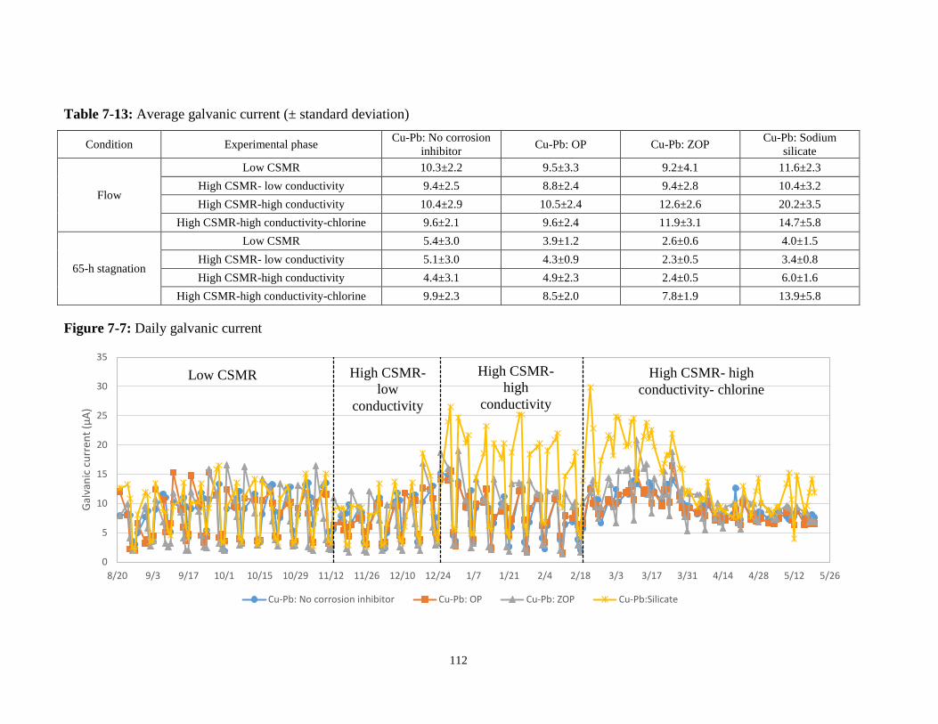
112

Table 7-13: Average galvanic current (± standard deviation)

Condition Experimental phase Cu-Pb: No corrosion


Cu-Pb: Sodium

silicate

Flow

Low CSMR 10.3±2.2 9.5±3.3 9.2±4.1 11.6±2.3

High CSMR- low conductivity 9.4±2.5 8.8±2.4 9.4±2.8 10.4±3.2

High CSMR-high conductivity 10.4±2.9 10.5±2.4 12.6±2.6 20.2±3.5

High CSMR-high conductivity-chlorine 9.6±2.1 9.6±2.4 11.9±3.1 14.7±5.8

65-h stagnation

Low CSMR 5.4±3.0 3.9±1.2 2.6±0.6 4.0±1.5

High CSMR- low conductivity 5.1±3.0 4.3±0.9 2.3±0.5 3.4±0.8

High CSMR-high conductivity 4.4±3.1 4.9±2.3 2.4±0.5 6.0±1.6

High CSMR-high conductivity-chlorine 9.9±2.3 8.5±2.0 7.8±1.9 13.9±5.8

Figure 7-7: Daily galvanic current

0

5

10

15

20

25

30

35

8/20 9/3 9/17 10/1 10/15 10/29 11/12 11/26 12/10 12/24 1/7 1/21 2/4 2/18 3/3 3/17 3/31 4/14 4/28 5/12 5/26

Gal

van

ic c

urr

ent

(µA

)

Cu-Pb: No corrosion inhibitor Cu-Pb: OP Cu-Pb: ZOP Cu-Pb:Silicate

Low CSMR High CSMR-

low

conductivity

High CSMR-

high

conductivity

High CSMR- high

conductivity- chlorine

113

Table 7-14: Water quality parameters of reservoir water (part 1)

Experimental

condition Systems pH

Conduc

tivity

(mS/cm

)

Chloride

(mg/L)

Sulfate

(mg/L) CSMR

Corrosion

Inhibitor

Added (mg/L)

Residual

chlorine

(mg/L)

TOC

(mg/L)

Acclimation

PVC-Pb: No corrosion inhibitor 7.9±0.0 NM 27.2±1.0 127.9±2.1 0.2±0.0 NA NA 2.7±0.1

Cu-Pb: No corrosion inhibitor 7.9±0.1 NM 27.0±0.8 127.9±1.8 0.2±0.0 NA NA 2.5±0.1

Cu-Pb: OP 7.9±0.1 NM 27.2±1.0 127.4±2.2 0.2±0.0 NA NA 2.7±0.1

Cu-Pb: ZOP 7.9±0.0 NM 27.3±1.1 127.6±2.7 0.2±0.0 NA NA 2.6±0.1

Cu-Pb: Sodium Silicate 8.0±0.2 NM 27.3±1.1 128.8±2.7 0.2±0.0 NA NA 2.7±0.1

Low CSMR

PVC-PVC: No corrosion inhibitor 7.9±0.1 533±2 27.3±1.8 133.8±3.2 0.2±0.0 NA NA 8.1±1.7

PVC-Pb: No corrosion inhibitor 7.9±0.1 545±5 26.8±1.9 135.6±4.7 0.2±0.0 NA NA 3.7±0.7

Cu-Pb: No corrosion inhibitor 7.9±0.1 546±3 27.0±1.7 137.2±3.9 0.2±0.0 NA NA 4.0±1.0

Cu-Pb: OP 7.9±0.1 552±6 27.1±1.7 136.5±3.4 0.2±0.0 1.0±0.1 NA 5.7±1.9

Cu-Pb: ZOP 7.9±0.0 558±5 27.5±1.9 137.3±2.9 0.2±0.0 0.9±0.1 NA 5.2±1.5

Cu-Pb: Sodium Silicate 8.0±0.2 543±2 27.2±1.9 134.6±2.8 0.2±0.0 10.1±1.0 NA 5.6±1.8

High CSMR

with low

electrical

conductivity




Cu-Pb: OP 7.9±0.1 336±10 30.2±0.9 26.9±0.7 1.1±0.0 0.9±0.1 NA 2.5±0.4

Cu-Pb: ZOP 7.9±0.1 337±10 30.7±0.9 26.9±0.7 1.1±0.0 0.9±0.0 NA 2.4±0.3


High CSMR

with high

electrical

conductivity




Cu-Pb: OP 7.9±0.1 573±20 85.8±4.9 81.4±2.1 1.1±0.1 1.0±0.1 NA 2.4±0.1

Cu-Pb: ZOP 7.9±0.1 573±22 86.1±4.7 81.7±1.5 1.1±0.1 1.0±0.1 NA 2.3±0.1


114

Table 7-14: Water quality parameters of reservoir water (part 2)

Experimental

condition Systems pH

Conducti

vity

(mS/cm)

Chloride

(mg/L)

Sulfate

(mg/L) CSMR

Corrosion

Inhibitor

Added (mg/L)

Residual

chlorine

(mg/L)

TOC

(mg/L)

High CSMR

with high

electrical

conductivity

PVC-PVC: No corrosion inhibitor 8.0±0.0 603±20 88.8±0.9 78.7±1.8 1.1±0.0 NA 1.4±0.2 3.3±0.6

PVC-Pb: No corrosion inhibitor 7.9±0.1 599±19 87.1±1.1 77.7±1.3 1.1±0.0 NA 1.4±0.2 2.7±0.4

Cu-Pb: No corrosion inhibitor 7.9±0.1 597±19 87.1±1.1 77.8±1.0 1.1±0.0 NA 1.4±0.2 2.5±0.7

Cu-Pb: OP 7.9±0.1 601±20 87.1±1.1 77.8±1.0 1.1±0.0 1.0±0.1 1.4±0.3 2.8±0.7

Cu-Pb: ZOP 7.9±0.1 603±19 86.4±1.0 75.9±0.8 1.1±0.1 1.1±0.1 1.4±0.2 3.0±0.8

Cu-Pb: Sodium Silicate 8.1±0.2 603±19 86.4±1.0 75.9±0.8 1.1±0.1 10.2±0.8 1.4±0.2 2.7±0.8

115

7.3 Preliminary Results

7.3.1 Tank Acidification

7.3.1.1 Materials and Methods

The objectives of this preliminary experiment were: i) to determine the time required to dissolve

all particulate lead in the reservoirs when acidified to pH < 2, ii) to examine the effect of

mechanical mixing during acidification, and iii) to compare two methods for sample preparation:

acid preservation and acid digestion.

Determination of Time to Completely Acidify Reservoir

Three reservoirs (Reservoirs 1, 2, and 3) (Figure 7-8), each holding 90 L of water, were acidified

to pH < 2 by adding concentrated nitric acid (67%). The amount of acid required to acidify each

tanks to pH < 2 was determined by titration prior to the experiment. To compare the

effectiveness of mixing, Reservoir 3 (Figure 7-8) was acidified to pH < 2 in the same way and

also received mechanical mixing at 320 rpm with a 22-inchTeflon® anchor-style paddle assembly

(Cole-Parmer Canada Inc., Montreal, QC).

Reservoirs 4 and 5 (Figure 7-8) were used to compare the effect of decreasing the volume of

water and determine the feasibility of acidifying a smaller volume. Water was drained to 20 L by

pumping water out of the reservoirs to waste.

A 10-mL sample was collected from all five reservoirs by inserting a volumetric pipette 6-cm

below the water surface at time = 0, 4, 20, 24, 26, and 30 hours post acidification.

Comparison of Two Sample Preparation Methods

10 mL of samples were collected from all reservoirs at time = 0, 24, and 30 hours following

acidification. Samples were digested with 0.5 mL of nitric acid at 105º C for 2 h, following the

Standard Method 3030 E (APHA, 2004). The two methods (preservation at pH < 2 and nitric

acid digestion) were then compared for lead recovery.

Measurement of Residual Lead in Reservoir after the First Acidification

116

Following reservoir acidification, a follow-up experiment was conducted to evaluate the

potential contribution of lead adsorption to the reservoir walls. Following the experiments, water

was pumped to waste. Reservoir 2 was washed thoroughly to evaluate the effectiveness of

cleaning. Three of the five reservoirs (# 1, 2, and 3) were then refilled with 90 L of Lake Ontario

water and acidified to pH < 2. This second acidification lasted for 24 h; samples were collected

at t = 0, 4, 24 h. Samples were collected 6-cm below the surface using a disposable plastic pipette

tip.

All samples obtained in the two experiments were analyzed for total lead using ICP-MS as

described in Section 3.2.1.

Figure 7-8: Treatments to Determine Lead Recovery from Reservoirs

7.3.1.2 Results

Experiments were conducted to determine the time required to dissolve all particulate lead in the

reservoirs when acidified to pH < 2. Three approaches were examined: 1) acidification of 90 L of

water, 2) acidification of 90 L of water with mechanical mixing by a 22-inch anchor-style paddle

assembly (320 rpm), and 3) acidifying only 20 L of the water. There was no significant

difference between these three approaches. The total lead concentrations in the samples ranged

from 136 to 350 µg/L. The average total lead concentrations in the samples ranged from 143 to

248 µg/L, and approximately 96% of data remained within ± 10% of the averages after 20 hours

of acidification (Figure 7-9). The result suggested that all lead in the reservoirs was dissolved

90 L 90 L

Reservoir 1 Reservoir 2 Reservoir 3

Reservoir 5 Reservoir 4

90 L

20 L 20 L

117

within 20 hours and that the reservoirs contained only limited amounts of particulate lead. The

difference in total lead presumably originated from difference in the harvested lead pipes. In

order to assess the contribution of particles to total lead, the preservation method (pH < 2) and

the nitric acid digestion method (105º C for 2 h) were compared and did not produce statistically

significant difference (95% CI), which implied a limited contribution of particulate lead. During

reservoir acidification, pH ranged from 1.63-1.96 throughout the 50-hour experiment, and

turbidity of the waters did not show a trend.

Following acidification experiment, three reservoirs were refilled with water and acidified to pH

< 2 to assess the amount of lead adsorbed to reservoir walls. One reservoir was left stagnant, a

second reservoir was cleaned with raw water and brushed with a plastic brush prior to

acidification, and the third reservoir received mechanical mixing during acidification. After 4

hours of the second acidification, the total lead concentration was within ± 10% of the average of

each reservoir and ranged from 0.18 to 2.78 µg/L. The third reservoir, which employed a

mechanical mixer whereas had the highest average total lead concentration (2.78 µg/L), and the

reservoir that received cleaning before the second acidification had the lowest average total lead

concentration (0.20 µg/L). The lead released from the reservoir walls was < 4% of the average

total lead concentrations of the first acidification samples.

118

Figure 7-9: Lead Concentrations During 50-h Acidification

0

50

100

150

200

250

300

350

400

0 10 20 30 40 50

Pb C

once

ntr

atio

ns

(µg/L

)

Time (h)

Reservoir 1 (90 L, No mixing)


Reservoir 3 (90 L, Mixing)



119

7.3.2 Chlorine Demand Test

7.3.2.1 Materials and Methods

Free chlorine demand test

Chlorine demand test was conducted using 1 L of waters from the six reservoirs to

determine whether the addition of corrosion inhibitors and other water matrix factors have any

effects on chlorine demand. Free chlorine residuals and pH of the waters from the six reservoirs

in 1-L beakers were monitored daily for 6 days with daily adjustment of chlorine concentrations.

The beakers used for this experiment were not processed for chlorine demand free, for the

reservoirs will not be prepared for chlorine demand free at the beginning of every weekly cycle.

The initial dose was 1.5 mg/L as Cl2, and the free chlorine concentrations in the waters were

raised to 1.5 mg/L by daily adjustment. Parallel to this experiment, a reservoir with 90 L of water

was used to determine if there is stratification of chlorine concentrations among the locations of a

reservoir (near surface, middle, and bottom). A pump was used to collect 1 L of water from the

middle and bottom of the reservoir, and 10 mL of each sample was used to determine total and

free chlorine concentrations. The same experiments using 1 L of waters and a reservoir with 90-

L water were repeated with an initial dose of 2.0 mg/L as Cl2, and the free chlorine concentration

was raised to 1.5 mg/L by daily adjustment. Samples were collected from the near surface

location of a reservoir because no stratification was observed in the first experiment.

7.3.2.2 Results

The free chlorine concentrations were monitored for 4 days. The initial dose of free

chlorine was 2.0 mg/L, and the concentrations were raised to 1.5 mg/L by daily adjustment from

Day 2. There was a large decrease in the free chlorine concentration of Cu-Pb: ZOP system on

the first day, but the results were similar to each other on other days (Figure 2).

120

Figure 7-10: Free chlorine concentrations in 1 L of waters from the six reservoirs (second time)

0.00

0.25

0.50

0.75

1.00

1.25

1.50

1.75

2.00

0 1 2 3 4 5

Fre

e c

hlo

rin

e (

mg/

L as

Cl2

)

Time (day)

Reservoir (90 L)

Cu-PVC: No corrosionInhibitorCu-Pb: No corrosioninhibitorCu-Pb: OP

Cu-Pb: ZOP

Cu-Pb: Silicate

PVC-PVC: Nocorrosion inhibotor

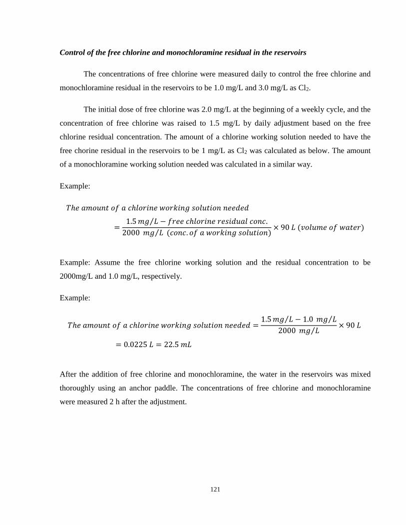
121

Control of the free chlorine and monochloramine residual in the reservoirs

The concentrations of free chlorine were measured daily to control the free chlorine and

monochloramine residual in the reservoirs to be 1.0 mg/L and 3.0 mg/L as Cl2.

The initial dose of free chlorine was 2.0 mg/L at the beginning of a weekly cycle, and the

concentration of free chlorine was raised to 1.5 mg/L by daily adjustment based on the free

chlorine residual concentration. The amount of a chlorine working solution needed to have the

free chorine residual in the reservoirs to be 1 mg/L as Cl2 was calculated as below. The amount

of a monochloramine working solution needed was calculated in a similar way.

Example:

𝑇ℎ𝑒 𝑎𝑚𝑜𝑢𝑛𝑡 𝑜𝑓 𝑎 𝑐ℎ𝑙𝑜𝑟𝑖𝑛𝑒 𝑤𝑜𝑟𝑘𝑖𝑛𝑔 𝑠𝑜𝑙𝑢𝑡𝑖𝑜𝑛 𝑛𝑒𝑒𝑑𝑒𝑑

=1.5 𝑚𝑔 𝐿⁄ − 𝑓𝑟𝑒𝑒 𝑐ℎ𝑙𝑜𝑟𝑖𝑛𝑒 𝑟𝑒𝑠𝑖𝑑𝑢𝑎𝑙 𝑐𝑜𝑛𝑐.

2000 𝑚𝑔 𝐿⁄ (𝑐𝑜𝑛𝑐. 𝑜𝑓 𝑎 𝑤𝑜𝑟𝑘𝑖𝑛𝑔 𝑠𝑜𝑙𝑢𝑡𝑖𝑜𝑛)× 90 𝐿 (𝑣𝑜𝑙𝑢𝑚𝑒 𝑜𝑓 𝑤𝑎𝑡𝑒𝑟)

Example: Assume the free chlorine working solution and the residual concentration to be

2000mg/L and 1.0 mg/L, respectively.

Example:

𝑇ℎ𝑒 𝑎𝑚𝑜𝑢𝑛𝑡 𝑜𝑓 𝑎 𝑐ℎ𝑙𝑜𝑟𝑖𝑛𝑒 𝑤𝑜𝑟𝑘𝑖𝑛𝑔 𝑠𝑜𝑙𝑢𝑡𝑖𝑜𝑛 𝑛𝑒𝑒𝑑𝑒𝑑 =1.5 𝑚𝑔 𝐿⁄ − 1.0 𝑚𝑔 𝐿⁄

2000 𝑚𝑔 𝐿⁄× 90 𝐿

= 0.0225 𝐿 = 22.5 𝑚𝐿

After the addition of free chlorine and monochloramine, the water in the reservoirs was mixed

thoroughly using an anchor paddle. The concentrations of free chlorine and monochloramine

were measured 2 h after the adjustment.

impact of corrosion inhibitors on lead release and biofilm ... · impact of corrosion inhibitors on...

Documents