impact of exchange rate volatility on growth and economic ... · the pakistan development review 44...

The Pakistan Development Review 44 : 4 Part II (Winter 2005) pp. 749–775

Impact of Exchange Rate Volatility on Growth and Economic Performance: A Case Study

of Pakistan, 1973–2003

TOSEEF AZID, MUHAMMAD JAMIL, and ANEELA KOUSAR*

I. INTRODUCTION

“Exchange rate” is the price of one currency in relation to another. In a slightly different perspective, it expresses the national currency’s quotation in respect to foreign ones. Thus, exchange rate is a conversion factor, a multiplier or a ratio, depending on the direction of conversion. It is believed that if exchange rates can freely move, it may turn out to be the fastest moving price in the economy, bringing together all the foreign goods with it.

In the existing literature, (most of the time) volatility comes with the exchange rate. Volatility is defined as “instability, fickleness or uncertainty” and is a measure of risk, whether in asset pricing, portfolio optimisation, option pricing, or risk management, and presents a careful example of risk measurement, which could be the input to a variety of economic decisions.

Volatility of exchange rates describes uncertainty in international transactions both in goods and in financial assets. Exchange rates are modeled as forward-looking relative asset prices that reflect unanticipated change in relative demand and supply of domestic and foreign currencies, so exchange rate volatility reflects agents’ expectations of changes in determinants of money supplies, interest rates and incomes.

As many developing countries have or are considering implementing changes in their development strategies, now is an opportune time to investigate the issue of weather alteration, in exchange rate arrangement have an effect on economic growth or to what extent exchange rate volatility may be responsible for variation in the rate of economic production. Because such moves are accompanied by increase in the volatility of both, nominal and real exchange rates [Caporale and Pittis 1995].

Toseef Azid is Professor of Economics, Markfield Institute of Higher Education (Loughborough University) Leicestershire, UK. Muhammad Jamil is Lecturer, Department of Economics, Bahauddin Zakariay University, Multan. Aneela Kousar is studying for her PhD at the Pakistan Institute of Development Economics, Islamabad.

Authors’ Note: We would like to thank Mr Ali Kemal of Pakistan Institute of Development Economics for his valuable comments on this paper.

Azid, Jamil, and Kousar 750

Real exchange rate uncertainty can have negative effects on both domestic and foreign investment decisions. It causes reallocation of resources among the sectors and countries, between exports and imports and creates an uncertain environment for investment. Two branches of macroeconomic theory relate to the question of how exchange rate volatility affects macroeconomic performance.

(1) The first examines how the domestic economy responds to foreign and domestic real and monetary shocks under different exchange rate regimes.

(2) The second focuses on the issue of how exchange rate volatility under flexible exchange rate regimes affects international trade.

In the case of free mobility of capital, an economy that is affected mainly by shocks to the LM curve, due to changes in money demand for example, will experience large fluctuations in output, inflation, and the exchange rate if the exchange rate is flexible.

If the exchange rate is fixed and capital is internationally mobile then the money supply is endogenous—changes in money demand determine changes in the money supply so that LM shocks will have no effect on output or inflation. Some recent work has certainly suggested that developing countries that peg their exchange rates achieve lower inflation than those whose exchange rate floats [Ghosh, et al. (1995); Aghevli, et al. (1991); Obstfeld (1995); Alogoskoufis (1992); Collins (1996); Bleaney and Fielding (1999)].

(1) The most important reasons for a devaluation to trigger an aggregate demand contraction include: a redistribution of income towards those with high marginal propensity to save, a fall in investment, an increased debt burden, reduction in real wealth, a low government marginal propensity to spend out of tax revenue, real income declines under an initial trade deficit, increased interest rates, and increased foreign profits [Diaz-Alejandro (1965); Cooper (1971, 1971a, 1971b); Krugman and Taylor (1978); Branson (1986); Buffie (1986a); Van Wijnbergen (1986); Gylfason and Risager (1984); Gylfason and Schmid (1983); Hanson (1983); Gylfason and Radetzki (1991); Barbone and Rivera-Batiz (1987)].

(2) On the other hand, aggregate supply may suffer after devaluation because of: more expensive imported production inputs, wage indexation programmes, costlier working capital [Bruno (1979); Gylfason and Schmid (1983); Hanson (1983); Gylfason and Risager (1984); Islam (1984); Gylfason and Radetzki (1985); Branson (1986); Solimano (1986); Van Wijnbergen (1986); Edwards (1989)].

(3) Increases in the volatility of the real effective exchange rate, exert a significant negative effect upon export demand in both the short-run and the long run and these effects may result in significant reallocation of

Impact of Exchange Rate Volatility 751

resources by market participants. The issue is particularly important for countries that Switched from a fixed to a flexible exchange rate regime due to the higher degree of variability associated with flexible exchange rates [Hooper and Kohlhagen (1978); Coes (1981); De Grauwe (1988); Brada and Mendez (1988); Caballero and Corbo (1989); Côté (1994); Baum, et al. (2001) and Arize, Osang, and Slottje (2004)].

(4) The impact of exchange rate volatility on investment and hence on economic growth is not a recent source of concern. It is noted in the literature that uncertainty reduces investment in the presence of adjustment costs and when the investment process includes irreversibilities. Real exchange rate uncertainty creates an uncertain environment for investment decisions and therefore, investors delay their investment decisions to obtain more information about the real exchange rates if investments are irreversible and exerts negatively on economic performance.

Campa and Goldberg (1993) found a negative impact of exchange rate volatility on investment. Whereas Aizenman (1992) finds positive relationship. While Campa and Goldberg (1995) find almost no impact.

Keeping such relationships in mind a hypothesis is developed relating to the link between exchange rate volatility and economic growth. It is considered an opportune time for such analysis because more and more countries are considering revisions in their exchange rate arrangements. Theory suggests a direct link between exchange rate volatility and economic performance in the presence of open economies. In such state of affairs the aim of the study is to find out the nature of this relationship, i.e. positive or negative or even insignificant.

The rest of the study is arranged as: Section II takes into discussion the empirical methodology employed and contain explanation about the construction and utilisation of variables. Section III discusses and analyses the results. And finally the last section contains summary and conclusions.

II. METHODOLOGY AND DATA DESCRIPTION

This section discusses the methodology employed to measure volatility, and the techniques suggested to capture the effects of volatility on economic performance. II.1. The Empirical Methodology II.1.1. Measurement of Volatility

When dealing with time varying measures of volatility in exchange rate series, economists construct a rolling (moving) variance of the series. However, the rolling variance is a naive derivation of uncertainty. It assumes that economic agents are not


necessarily exploiting patterns in the data when making forecasts of uncertainty and measures fluctuations of the exchange rate but not the uncertainty in exchange rate [Dorantes and Pozo 2001].

The choice stands for GARCH as a measure of uncertainty that forecasts exchange rate movements and measure uncertainty around that forecast. ARCH stands for autoregressive conditional heteroscedasticity.

(1) Autoregressive describes a feedback mechanism that incorporates past observations into the present,

(2) Conditional implies a dependence on the observations of immediate past, and

(3) Heteroscedasticity represents a time-varying variance (i.e., volatility).

Therefore, ARCH Models allow the error term to have a time varying variance i.e. to be conditional on the past behaviour of the series. ARCH models were introduced by Engle (1982) and generalised as GARCH (Generalised ARCH) by Bollerslev (1986) that offer a more parsimonious model (i.e., using fewer parameters) that lessons the computational burden [Bollerslev, Chou, and Kroner (1992) and Bollerslev, Engle, and Nelson (1994)]. These models are widely used in various branches of econometrics, especially in financial time series analysis [Kroner and Lapstrapes (1994); Grier and Perry (2000); Arize (1998); Glistens, et al. (1993)]. The application of GARCH provides variable of interest i.e. the exchange rate volatility. II.1.2. Stationary/Unit Root Test

The first step of the empirical process involves a test for unit roots. This is necessary because the co-integration tests can be applied only to variables that are non-stationary in levels (contain a unit root). Dickey and Fuller (1979, 1981) and Said and Dickey (1984) have developed a method to determine whether a variable contains a unit root. The tests are conducted, including a drift term and both with and without a trend. The inclusion of a trend allows testing that whether the series is trend or difference stationary [Amuedo and Pozo (2001); Sinha (1999); Pesaran and Smith (1998)].

II.1.3. VAR and Cointegration Test

Applying test for stationary and confirming stationary otherwise leads to VAR (Vector Autoregressive Model) constructed in order to take account of all the dynamic and co-integrating interrelationships and impact of random disturbances on the system of variables that result in forecasting systems of interrelated time series. Granger Causality test (1969) is used to see any cause and effect relationship between variables, (how much of the current value of a dependent variable can be explained by past values of that variable and testing whether adding lagged values of independent can improve the explanation).


Movement on such smooth track leads to “co-integration” that implies identifying the co-integrating (long-run equilibrium) relationships. Using the methodology developed by Johansen (1991, 1995). Co-integration implies that stationary linear combinations of non-stationary variables exist.1 The central concept of co-integration is the specification of models that include the long-run movements of one variable relative to others, the test require an appropriate VAR specification among the variables of interest [Joyce and Kamas (1994); Alexakis and Apergis (1994); Bahmani-Oskooee and Alse (1995); Cifarelli (1995); Faruqee (1995) and Sinha (1999)]. II.1.4. Variance Decomposition and Impulse Response Functions

Finally to infer the dynamic relationship among variables in the modal the variance decomposition along with the IRFs (impulse response function) are performed.

IRFs [Hamilton (1994)] trace the effects of a shock to an endogenous variable in VAR. IRF traces the effect of a one standard deviation shock to (innovations) current and future values of the endogenous variables due to the fact that a shock to the ith variable directly affects the ith variable, and is also transmitted to all of the endogenous variables through the dynamic structure of the VAR.

Whereas, variance decomposition decomposes variation in an endogenous variable into the component shocks in the VAR, and provide information about the relative importance of each random innovation to the variables in the VAR. II.2. Data Sources and Construction of Variables

The variables in the analysis are real money (RM), the real exchange rate (RER), real exchange rate volatility (VOL), exports (EX), imports (IM), and manufacturing production indexes (Y). Because the approach necessities the use of high frequency data, the analysis is constrained to using narrow measure of economic production i.e. manufacturing production indexes as used by Dorantes and Pozo (2001).

The series are constructed as follows. The real exchange rate is the relative inflation adjusted exchange rate, and is constructed by multiplying the nominal exchange rate by the ratio of consumer price indexes (e.g. RER=(PAK/USA)*(CPI US/CPI PAK)). The real exchange rate volatility (VOL) i.e. the variables of interest is computed by using GARCH model.

The real money supply series are obtained by deflating the money supply series with the consumer price indexes; CPIs are converted into common base of 1995. The exports and imports are taken on unit values with common base of 1995. As a measure of output (RY) the manufacturing production series is used.2 Prior to

1In this study we have used the methodology developed by Engle and Granger. 2It is assumed that manufacturing indices underestimate the true GDP but at the time of this study

the relevant data were not available.


the estimation all variables are transformed into natural logarithms, with the exception of real exchange rate volatility.

Data span from 1973-Q1 to 2003-Q4, providing series of 120 observations. All the series expect the manufacturing production are obtained from

international financial statistics (IFS) up to 1998, from 1998 to 2003 the series are obtained from Statistical Bulletin of Government of Pakistan, Finance Division. Data regarding manufacturing indexes are obtained from statistical bulletin. II.3. Variables Performance Over Time II.3.1. Real Exchange Rate

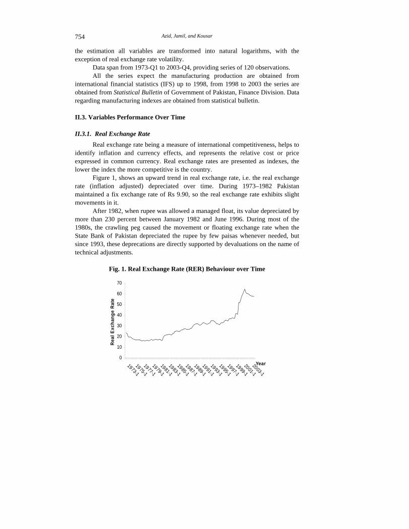
Real exchange rate being a measure of international competitiveness, helps to identify inflation and currency effects, and represents the relative cost or price expressed in common currency. Real exchange rates are presented as indexes, the lower the index the more competitive is the country.

Figure 1, shows an upward trend in real exchange rate, i.e. the real exchange rate (inflation adjusted) depreciated over time. During 1973–1982 Pakistan maintained a fix exchange rate of Rs 9.90, so the real exchange rate exhibits slight movements in it.

After 1982, when rupee was allowed a managed float, its value depreciated by more than 230 percent between January 1982 and June 1996. During most of the 1980s, the crawling peg caused the movement or floating exchange rate when the State Bank of Pakistan depreciated the rupee by few paisas whenever needed, but since 1993, these deprecations are directly supported by devaluations on the name of technical adjustments.

Fig. 1. Real Exchange Rate (RER) Behaviour over Time

0

10

20

30

40

50

60

70

1973-1

1975-1

1977-1

1979-1

1981-1

1983-1

1985-1

1987-1

1989-1

1991-1

1993-1

1995-1

1997-1

1999-1

2001-1

2003-1

Year

Rea

l Exc

hang

e R

ate


Frequent devaluation stimulates speculation, leading to confidence erosion. Such practice of continuous devaluation not only result in distortions in income, consumption, industrial growth and public finance, but also disturb the harmonious blend of internal and external balance, affecting both monetary and fiscal indicators, e.g. exports, imports, manufacturing growth, money supply and so on.

After July 2001, the government decided for the free-floating of the exchange rate, which result in drastic changes in real exchange rate, and after reaching almost its maximum of Rs 64 in 2002, shows a downward trend (appreciation) when the market forces played well in favour of Pakistan. The continued build up in foreign exchange reserves, surplus in current account balance and increased inflow remittances through banking channel has strengthened Pakistani rupee via US dollar. In both open market and interbank market rupee appreciated 3.25 percent and 3.49 percent respectively during the period of study. Figure 2 depicts the trends in real exchange rate uncertainty/volatility.

Fig. 2. Exchange Rate Volatility (VOL) over Time

0.0000

0.0005

0.0010

0.0015

0.0020

0.0025

1982-1

1983-2

1984-3

1985-4

1987-1

1988-2

1989-3

1990-4

1992-1

1993-2

1994-3

1995-4

1997-1

1998-2

1999-3

2000-4

2002-1

2003-2

Year

Exch

ange

Rat

e Vo

latil

ity (V

OL)

II.3.2. Exports

“Exports” representing the sales in other countries, generate foreign currency earnings, and boost economic growth. Demand for exports depends on economic conditions in foreign countries, prices (relative inflation and exchange rate), and perception of quality, reliability, and so on.

According to the orthodox approach, the devaluation enhances competitive-ness, increases exports and bends demand toward domestically produced goods, thus expanding the production of tradable. However, frequent output declines in the

Exc

hang

e R

ate

Vol

atili

ty (V

OL

)

Year


aftermath of devaluations hinted that the benign relative price adjustment caused by devaluations could bring about a recession. For demand and supply side contractionary effects [Diaz-Alejandro (1963); Krugman and Taylor (1978); Barbone and Rivera-Batiz (1987)], the studies of supply side include [Bruno (1979); Gylfason and Schmid (1983); Van Wijnbergen (1986); Agenor (1991); Gylfason and Radetzki (1991) and Taye (1999)].

In 1972-73 after 21 successive years of unfavourable balance of trade, Pakistan achieved surplus due to deliberate policy of devaluation and export promotion measures. Pakistan’s exports are highly concentrated in cotton, leather, rice, synthetic textiles and sports goods. These five categories accounted for 82.6 percent of total exports during 2002-03. Pakistan trades with a large number of countries but its exports are highly concentrated with USA, Germany, Japan, the UK, Hong Kong, Dubai and Saudi Arabia. Among these countries, the maximum export proceeds are from the USA making up approximately 24 percent of the total.

Figure 3 shows an upward or increasing trend for Pakistani exports, with favourable composition changing for manufacturing and semi-manufacturing exports and a decreasing share of primary exports. On July 2001, the share of these sectors was 75 percent, 14 percent, and 11 percent respectively, because at international level the prices of manufactured items are more stable than primary products. Exports show drastic change in 1990s, when not only the internal and external factors affected heavily, a very strong factor causing drastic variations was the exchange rate arrangement of “managed floating”, where the government continuously changed the value of Pakistani rupee. After free floating of rupee in July 21, 2000, the variations were smoothed out again. Moreover, during 2003 the exports grew by 10.3 percent.

Fig. 3. Exports Movement over Time

0

20

40

60

80

100

120

140

160

1973-1

1975-2

1977-3

1979-4

1982-1

1984-2

1986-3

1988-4

1991-1

1993-2

1995-3

1997-4

2000-1

2002-2

Year

Uni

t Val

ue o

f Exp

orts

(EX)

Uni

t Val

ue o

f Exp

orts

(EX

)

Year


II.3.3. Imports

“Imports” measuring purchases from abroad, add to well being but may displace domestic production and drain financial resources. Changes in imports prices reflect changes in foreign prices, exchange rates and quantity.

Like exports, Pakistan’s imports are also highly concentrated in a few items namely, machinery, petroleum and petroleum products, chemicals, transport equipments, edible oil, iron and steel, fertiliser and tea. These eight categories of imports accounted for 75.9 percent of total imports during 2002-03.

Imports for Pakistan increases overtime including both consumer and capital goods. However, consumer goods increase more rapidly than capital goods, which are a prerequisite for long term self-sustained growth of the economy. The share of raw materials for consumer goods in the total imports continued to be high while that for capital goods remained low. The percentage share of industrial raw material has declined from 11 percent in 1969-70 to 5 percent in 2000-01. The share of capital goods exhibited a declining trend—mainly because of a slow down in investment in the country. Now started pick up because of a revival in the domestic economy. During the 2003, the share of consumer goods did not show any change and remained at 10 percent while that of raw materials for consumer goods came to 51 percent from 55 percent. However, due to higher imports of machinery, the share of capital goods increased from 29 percent to 32 percent. The share of raw material for capital goods showed an improvement of one percentage point during this period and stood at 7 percent. Figure 4 depicts that imports show a continuous upward trend, throughout 1970s to early 1990s, due to WTO pressure for liberalised import policy. During 2003, imports grew by 27.6 percent.

Fig. 4. Imports Movement over Time

0

20

40

60

80

100

120

140

1973-1

1975-2

1977-3

1979-4

1982-1

1984-2

1986-3

1988-4

1991-1

1993-2

1995-3

1997-4

2000-1

2002-2

Year

Uni

t Val

ue o

f Im

port

s (IM

)

Uni

t Val

ue o

f Im

port

s (IM

)

Year


II.3.4. Money

Money being the corner stone of modern economy provides a bridge between the nominal and real magnitudes. Measured in notes, coins and various bank deposits; it works as an indicator of level of transactions, inflation and output. Money supply in Pakistan shows a smooth upward trend in its growth, which gets momentum after year 2000.

During 1999 and 2000, the monetary policy stance remained tight to keep inflation under control and bring stability in exchange rate to preserve export competitiveness. This policy stance has been eased since 2001 to promote investment and growth. During 2002-2003, the annual growth rate of money was 16.8 and 18.4 percent respectively (see Figure 5).

Fig. 5. Real Money Supply Movement over Time

0

5000

10000

15000

20000

25000

30000

35000

1973-1

1975-2

1977-3

1979-4

1982-1

1984-2

1986-3

1988-4

1991-1

1993-2

1995-3

1997-4

2000-1

2002-2

Year

Real

Mon

ey S

uppl

y

II.3.5. Manufacturing Production

Manufacturing production measures the value-added output of manufacturing sector, and an indicator of industrial activity. Manufacturing sector is the second largest individual sector of the economy accounting for 18 percent of gross domestic product (GDP).

Fig. 6. Manufacturing Sector Behaviour over Time

0

50

100

150

200

250

300

350

400

1973-1

1975-2

1977-3

1979-4

1982-1

1984-2

1986-3

1988-4

1991-1

1993-2

1995-3

1997-4

2000-1

2002-2

Year

Man

ufac

turi

ng In

dex

(Y)


Pakistan developed a substantial industrial sector in a very short period. During 1970s, the growth rate of GDP shows a decreasing trend and fell to 4.84 percent. The manufacturing sector growth rate was also low due to policy of nationalisation. During 80s, the industrial policy laid greater emphasise on employment generation, export promotion and increased efficiency of production units. Consequently, the manufacturing sector grew annually at a rate of 7.3 percent as compared to 5.4 percent in the previous decade and rose to 8.26 in 1991-92. During 1990s owing to a host of problems like tariff reforms and escalating utility prices, the growth remains lackluster. The growth rate of 4.0 percent was disappointing during 1990s. Since 1987-88, the year 2002 became the best performing year for manufacturing with growth rate of 7.7 percent. The contribution of manufacturing in GDP has increased overtime, from 6 percent in 1970-71 to 122 percent in 2001-2002. The above explanation can be seen in Figure 6.

III. RESULTS AND DISCUSSION

Unit Root Test

The data for this study exhibits the regular characteristics associated with most Macroeconomic variables. This conclusion derives from the unit root tests carried out on the variables used. Checking stationary is necessary because during building models for time series, the underlying stochastic process that generated the series must be invariant with respect to time. If the characteristics of the stochastic process change over time, i.e., if the process is non-stationary, it will often be difficult to represent the time series over past and future intervals of time by a simple algebraic model. This lead to misleading result.3

On the other hand, if the stochastic process is fixed in time, i.e., if it is stationary, then one can model the process via an equation with fixed coefficients that can be estimated from past data. We report the results for the ADF test because it has an Over-riding advantage on the series, as ADF automatically controls for higher order correlations by assuming that the coefficient of the series follows an AR (p) process and automatically adjusts the test methodology. Results of ADF tests shows that all the variables of the model are integrated at I (1), suggesting the need for differencing of the variables. This means that we can precede with the Johansen co-integration tests for these variables. Table 1 contains the results from the unit root test.

3We also applied the PP test but no different results were observed.


Table 1

Unit Root Tests of the Variables ADF Test Statistics PP Test Statistics

Intercept Trend and Intercept Intercept Trend and Intercept

Variables Level First

Difference Level First

DifferenceLevel First


Difference RER –0.6366 –3.7790* –2.3553 –3.7572* –0.6769 –8.8883* –1.8599 –8.8420* EX –0.0250 –4.9881* –1.6760 –4.9879* –0.4416 –103147* –2.7596 –10.2563* IM –0.1563 –5.0260* –2.5227 –5.0060* –0.5021 –10.4757* –3.7167 –10.4133* RM 1.9635 –3.5333* 0.4964 –4.1240* –0.8706 –14.5910* –4.0738 –14.5130* Y –0.2021 –3.8513* –1.8023 –3.8521* 1.9392 –9.6106* 0.2139 –10.0051*

1% –3.4681 –4.0373 –3.4865 –4.0380 –3.5604 –4.0661 –3.5073 –4.0673

5% –2.8857 –3.4478 –2.8859 –3.4481 –2.8947 –2.8951 –3.4614 –3.4620

Clin

ical

V

alue

s

10% –2.5795 –3.1488 –2.5796 –3.1489 –2.5942 –3.1567 –2.5844 –3.1570 *Series is Stationary.

Application of ARCH/GARCH for “Volatility”

The variable of Volatility is a measure of risk, which is generated through ARCH/GARCH process, allowing the error term to have a time varying variance. Table 2 shows the results.

Table 2

ARCH/GARCH Specification for Volatility Dependent Variable: D (LOG (RER))

Method: ML–ARCH Sample (adjusted): 1983:1 2003:4 Included Observations: 84 after Adjusting Endpoints Convergence Achieved after 77 Iterations

Coefficient Std. Error z-Statistic Prob. C 0.007764 0.005047 1.538148 0.1240

AR(3) 0.257173 0.121361 2.119068 0.0341 Variance Equation

C 6.08E-06 2.04E-05 0.298448 0.7654 ARCH (1) –0.044754 0.008760 –5.108715 0.0000

GARCH (1) 1.053971 0.035410 29.76473 0.0000 R-squared 0.105030 Mean dependent var 0.011572 Adjusted R-squared 0.059715 S.D. dependent var 0.036007 S.E. of Regression 0.034916 Akaike info criterion –4.153220 Sum Squared Resid. 0.096309 Schwarz criterion –4.008528 Log Likelihood 179.4352 F-statistic 2.317785 Durbin-Watson Stat 1.845568 Prob (F-statistic) 0.064288 Inverted AR Roots .64 –.32+. 55i –.32 –.55i


Correllogram of the series indicate the existence of autocorrelation and partial autocorrelation up to three lags, indicating the pattern of temporal dependence in the series, with p-value 0.009, indicating spurious results. The inclusion of AR (3) solve the problem of correlation and provide the variable of interest i.e., Volatility. Testing for unit root indicate that the variable is stationary at first difference, i.e. I (1) (see Table 3).

Table 3

Unit Root Test of Volatility Variable ADF Test Statistics PP Test Statistics

Intercept Trend and Intercept Intercept Trend and Intercept

Variable Level First




Difference Vol –1.8485 –3.6855* –1.6956 –3.7532* –1.7671 –9.7126 –1.5551 –9.7445

Critical values are used from Table 1. * Series is stationary.

Granger Causality and VAR

To account for both feedback and dynamic effects, and to facilitate a meaningful interpretation of any long run relationships among the series we chose a VAR framework for our analysis. In estimating, a VAR there is a choice between a large model, which captures all of the possible forces affecting variables of interest, and a more parsimonious model, which uses less degree of freedom and enables estimation that is more efficient. Given the aim of estimating the impact of the exchange rate volatility on output (manufacturing sector), it is common to choose a small, three or four variable model. Given the available data, it is felt that a three variable model including the real exchange rate, volatility, and manufacturing product will best describe the relationship between variables. The volatility picks up the effect of exogenous and endogenous shocks on the manufacturing product, while the real exchange rate will pick up the impact of domestic monetary policy on output. Finally, the manufacturing product variable will pick up all of the other shocks, which affect GDP.

The ordering of variables is important for impulse response functions. Since there is no specific theory of how to determine a causal structure, the order of the variable can be arbitrary. Usually, theoretical motivation or even data arability motivation is used to order the variables. However, the specific order can have major consequences for the policy implications of a model.4 Therefore, it is important to check if alternative ordering gives significantly different results. Choosing an appropriate lag length is also important, since too many lags reduce the degree of freedom, while too short a lag structure may lead to serial correlation in error terms, which can result in spurious significance and inefficient estimates.

4See Pindyck and Rubinfeld (1998) for detail.


The procedure of choosing the lag length is based on use of Akaike Information Criteria (AIC), the Schwartz Bayesian Criterion (SBC) and Hannan-quinn criterion (HQC). It is observed that the AIC tends to prefer longer lags while SBC and HQC tend to choose shorter lags; in this analysis the choice stands for SBC. The value of R2 is 0.950834. Therefore, 95 percent variations in each of the variables can be interpreted by the lagged values of all the endogenous variables.

Within a VAR framework, Granger causality is characterised by a finite number of linear restrictions on a subset of parameters. Granger causality is a measure of the significance of one variable in forecasting another. To find out any cause and effect relationship between manufacturing product, real exchange rate, and volatility the granger causality test is applied. The results are not in favour of the relationship among these variables. We have checked the granger causality under the lag lengths of 1 to 6 for the above three variables. The results of Granger causality test are given in Table 4. The results showed that manufacturing product and volatility does not granger cause at any lag length, indicating that both the variables are independent. The results for real exchange rate and manufacturing product exhibits that at lag lengths 1 and 2 causality is bi-directional and at lag lengths 3, 4, 5, and 6 only manufacturing productivity does granger cause real exchange rate.

Table 4

Granger Causality Tests between Manufacturing Productivity, Volatility, and Real Exchange Rate

Lag Lengths Null Hypothesis 1 2 3 4 5 6 LP_Y does not

Granger Cause Vol 1.38564 1.03773 0.79719 0.49741 0.48711 0.43662 Vol does not Granger

Cause LP_Y 0.81375 0.46229 0.69771 0.99489 0.71539 0.38470 LP_RER does not

Granger Cause LP_Y 20.7207* 8.13809* 1.45101 0.51851 0.89355 1.64944 LP_Y does not

Granger Cause LP_RER 8.44616* 4.25034* 3.89092* 4.11184* 3.94662* 3.47908*

* P-value is less than .05 indicates rejection of null hypothesis.

The results appeared contrary to the theory, which suggests that exchange rate variations effects manufacturing production, positively or negatively depending upon the underlying facts. In a microeconomic context, at the level of the firm, the exchange rate variations directly affect the firm’s decisions to take up production or not. However, in a macro-economic context, the relationship is more likely to be bi-directional. Suggesting that the real exchange rate might have an indirect effect through its impacts on cost of domestic to foreign goods, leading to import


substitutions. Although the characterisation of causality is invariant to stationary properties of the series, the statistical inference under non-stationary and/or co- integrated systems is driven by very irregular asymptotic properties for which the usual critical values remain valid only under special conditions.

For all the VARs considered, we can never accept that volatility adds significant contribution to manufacturing product. Variance Decomposition and Impulse Response Functions

The dynamic relationships among the variables in the three variable models can be inferred from the variance decomposition along with the impulse response functions. Theory suggest that the real exchange rate and production series should be co-integrated because real exchange rate depreciations lowers the relative costs of domestic to foreign goods, causing import substitution to take place and promoting exports. Such effect would tend to increase the level of production.

Considering the following equations to check whether cointegration relationship exists among variables manufacturing product and volatility and manufacturing product and real exchange rate.

VolYLP 11_ β+α=

Results of the linear regression of the variables manufacturing product, volatility and real exchange rate are given in Table 5. The coefficient value is 322.2278, indicating that a 1 percent variation in volatility, contributes positively up to 322.2278 percent. However, the low value of R2 i.e. 0.161294, suggests that the independent variable cannot explain many of the time series of manufacturing product. On the other hand value of R2 i.e. 0.857717 suggests that independent variable explain many of the time series of manufacturing product.

Table 5

Linear Regression between Manufacturing Product, Volatility, and Real Exchange Rate

Independent Variable Dependent Vol LP_RER Variable α1 β1 α2 β2 LP_Y 3.5379* 322.2278* –3.194182* 1.987633* R2 0.061294 0.857717

*Significant at 5 percent level of significant.

If linear combination of the variables is integrated of order less than the integration of the variables then it implies cointigration exists. The unit root test is applied to check the level of stationary of the linear combination of the variables


(residual terms) on both Intercept and Trend and Intercept. Error terms for the first regression is stationary at first difference and series of residuals (e1) is integrated of order one while error term for the second regression (e2) is stationary at level and the series of residual is integrated of order zero i.e. I (0).

Table 6

Unit Root Test for the Error Term ADF Test Statistics PP Test Statistics

Intercept Intercept Variable Level First Difference Level First Difference e1 –0.3364 –9.2619* –0.7684 –14.1524* e2 –3.4702* – –7.9724* –

e1 Residuals obtain by linear regression between LP_Y and Vol. e2 Residuals obtain by linear regression between LP_Y and LP_RER. * Series is stationary.

As all the variables manufacturing product, volatility and real exchange rate integrated of first order only the series of residuals (e2) is integrated of order zero, this implies the co-integration relationship between the variables manufacturing product and real exchange rate. This leads to the estimation of error correcting equations, regressing difference of the log(RER) on the previous value of error term and similarly difference of log (y) on the previous value of error term ( 2e (–1)). Here the value of

α2 = –3.194182 β2 = 1.987633

While in the adjustment equations a = –0.468990 and b = 0.042996.

( ) ( )( )( )[ ] 0554450.0987633.1042996.0468990.0)( 2 <−=−−=β−ba

The value of )( 2β−ba < 0, so the error correction process is a stabilising process, and long run adjustment process exist. Sign of “a” is negative showing that output by itself contributes positively to readjustment process. The co-efficient “b” of error correction model is also positive. Which shows that adjustment through real exchange rate positively contribute to output.

Impulse responses are estimated to evaluate shock dynamics. Which provide distinct and complementary information. Non-zero impulse responses from one variable to another need not imply the presence of Granger causality, and vice versa [Dufour and Tessier (1993); Dufour and Renault (1998)]. Even though Granger causality analysis is a useful tool for analysing dynamic structures between time series, it cannot provide an estimate of the direction (sign) or magnitude of the relationships of interest.


This is why Sims (1980) proposed to invert the autoregressive part of the process and to work with the underlying moving-average representation. The VARs are similar to the ones in the previous section. However, the inversion procedure calls for a stationary VAR process, which can be set up by differencing every integrated variable included in the system. To evaluate the potential impact of different shocks on manufacturing product, we consider the following causality structures.

log (RER). log (y) (Structure 1) Vol. log (y) (Structure 2)

For these two variable systems, we are interested in shocks affecting the manufacturing production. The impulse response functions are given in Appendix A, B and C. The impulse functions for volatility resulting from manufacturing production turn out to be insignificants. In contrast, for all cases, real exchange rate shocks appear to have a significant impact on manufacturing production, with the expected positive sign.

IV. SUMMARY AND CONCLUSION

The advantages and disadvantages of different exchange rate regimes have inevitably spawned a massive literature [e.g. Aghevli, et al. (1991); Obstfeld (1995)].

Over the years flexible exchange rate arrangements (encouraging market forces to play without fear of intervention) have positively affected in a detectable way to the pace of economic performance. Though we cannot measure the effect of exchange rate uncertainty on GDP growth, we obtain evidence on its effects by tracing the impact of exchange rate uncertainty on manufacturing production as done by Dorantes and Pozo (2001).

Instead of using rolling variance to capture uncertainty, the study employ conditional estimate of the variable of interest, exchange rate uncertainty. This methodology allows for more of the past information to be incorporated and provide us with measure of uncertainty that is less naive than other measures commonly employed in the literature, i.e. standard deviation, rolling variance etc.

Applying unit root suggested that all the variables are stationary at first difference, i.e. I (1). We construct VAR; including three variables to differentiate between the hypotheses that exchange rate uncertainty depresses vs. promote manufacturing production. The results obtained are positive but are insignificant, and do not support the position that excessive volatility or shifting of exchange rate regimes has pronounced affects for manufacturing production. These results are consistent with what we obtain from the impulse responses.

The concerns raised by the policy-makers about the costs of adopting flexible exchange rate systems are not borne out by results.


In the previous empirical work, a negative link between exchange rate volatility and economic growth seems to prevail. Most of the previous studies used cross sectional data. Here we prefer time series to capture exchange rate uncertainty.

One can never provide definite proof of a negative proposition. It is believed, however, that this study adds to the body of evidence suggesting that exchange rate variability has no significant effect on manufacturing product.

Appendices

APPENDIX A

IMPULSE RESPONSE FUNCTION OF MANUFACTURING PRODUCT AND REAL EXCHANGE RATE

-0. 02

0. 00

0. 02

0. 04

0. 06

0. 08

0. 10

5 10 15 20 25 30 35 40 45 50

Res pons e o f LOG(RER) to LOG(RER)

-0. 02

0. 00

0. 02

0. 04

0. 06

0. 08

0. 10

5 10 15 20 25 30 35 40 45 50

Res pons e o f LOG(RER) to LOG(Y)

-0. 05

0. 00

0. 05

0. 10

0. 15

0. 20

0. 25

5 10 15 20 25 30 35 40 45 50

Res pons e o f LOG(Y) to LOG(RER)

-0. 05

0. 00

0. 05

0. 10

0. 15

0. 20

0. 25

5 10 15 20 25 30 35 40 45 50

Res pons e o f LOG(Y) to LOG(Y)

Response to One S.D. Innovations ± 2 S.E.

Response to One S. D. Innovation + 2 S.E. Response of LOG(RER) to LOG(RER) Response of LOG(RER) to LOG(Y)

Response of LOG(Y) to LOG(RER) Response of LOG(Y) to LOG(Y)


APPENDIX B

IMPULSE RESPONSE FUNCTION OF MANUFACTURING PRODUCT AND VOLATILITY

-0. 0002

-0. 0001

0. 0000

0. 0001

0. 0002

0. 0003

5 10 15 20 25 30 35 40 45 50

Res pons e o f VOL to VOL

-0. 0002

-0. 0001

0. 0000

0. 0001

0. 0002

0. 0003

5 10 15 20 25 30 35 40 45 50

Res pons e o f VOL to LOG(Y)

-0. 1

0. 0

0. 1

0. 2

0. 3

5 10 15 20 25 30 35 40 45 50

Res pons e o f LOG(Y) to VOL

-0. 1

0. 0

0. 1

0. 2

0. 3

5 10 15 20 25 30 35 40 45 50

Res pons e o f LOG(Y) to LOG(Y)

Response to One S.D. Innovations ± 2 S.E.

Response to One S. D. Innovation + 2 S.E.

Response of VOL to VOL Response of VOL to LOG(Y)

Response of LOG(Y) to VOL Response of LOG(Y) to LOG(Y)


APPENDIX C

IMPULSE RESPONSE FUNCTION OF MANUFACTURING PRODUCT AND VOLATILITY

-0 .0002

-0.0001

0.0000

0.0001

0.0002

5 10 15 20 25 30 35 40 45 50

Response of VO L t o VO L

-0.0002

-0.0001

0.0000

0.0001

0.0002

5 10 15 20 25 30 35 40 45 50

Response of VO L t o LO G ( RER)

-0.0002

-0.0001

0.0000

0.0001

0.0002

5 10 15 20 25 30 35 40 45 50

Response of VO L t o LO G ( Y)

-0.06

-0.04

-0.02

0.00

0.02

0.04

0.06

5 10 15 20 25 30 35 40 45 50

Response of LO G ( RER) t o VO L

-0.06

-0.04

-0.02

0.00

0.02

0.04

0.06

5 10 15 20 25 30 35 40 45 50

Response of LO G ( RER) t o LO G ( RER)

-0.06

-0.04

-0.02

0.00

0.02

0.04

0.06

5 10 15 20 25 30 35 40 45 50

Response of LO G ( RER) t o LO G ( Y)

-0.1

0.0

0.1

0.2

0.3

5 10 15 20 25 30 35 40 45 50

Response of LO G ( Y) t o VO L

-0.1

0.0

0.1

0.2

0.3

5 10 15 20 25 30 35 40 45 50

Response of LO G ( Y) t o LO G ( RER)

-0.1

0.0

0.1

0.2

0.3

5 10 15 20 25 30 35 40 45 50

Response of LO G ( Y) t o LO G ( Y)

Response t o One S. D. I nnovat ions ± 2 S. E.

REFERENCES

Agenor, P. R. (1991) Output, Devaluation, and the Real Exchange Rate in Developing Countries. Weltwirts chaftliches Archive 127, 18–41.

Aghevli, B. B., S. K. Mohsin, and P. J. Montiel (1991) Exchange Rate Policy in Developing Countries: Some Analytical Issues. Washington, D. C.: International Monetary Fund. (Occasional Paper No. 78.)

Aizenman, J. (1992) Exchange Rate Flexibility, Volatility and the Patterns of Domestic and Foreign Investment. IMF Staff Papers, December 1992, 890–922.

Response of One S. D. Innovations + 2 S.E.

Response of VOL to VOL Response of VOL to LOG(RER) Response of VOL to LOG(RER)

Response of LOG(RER) to VOL Response of LOG(RER) to LOG(RER) Response of LOG(RER) to LOG(Y)

Response of LOG(Y) to VOL Response of LOG(Y) to LOG(RER) Response of LOG(Y) to LOG(Y)


Aizenman, J. (1994) Monetary and Real Shocks, Productive Capacity and Exchange Rate Regimes. Economics 61:244, 407–34.

Alexakis, P., and N. Apergis (1994) The Feldstein-Horioka Puzzle and Exchange Rate Regime: Evidence from Cointegration Test. Journal of Policy Modeling 16, 459–472.

Alogoskoufis, G. S. (1992) Monetary Accommodation, Exchange Rate Regimes and Inflation Persistence. Economic Journal 102, 461–80.

Amuedo-Dorantes, C., and S. Pozo (2001) Exchange-Rate Uncertainty and Economic Performance. Review of Development Economics 5:3, 363–74.

Arize, A. T. O., and D. Slottje (2004) Exchange Rate Volatility and Foreign Trade: Evidence from Thirteen LDCs. Journal of Business and Economic Statistics 18, 10–17.

Arize, A. C. (1998) The Effects of Exchange Rate Volatility on U.S. Imports: An Empirical Investigation. International Economic Journal 12:3, 31– 40.

Bahmani-Oskooee, M., and J. Asle (1995) Is There any Long-Run Relation Between the Terms of Trade and the Trade Balance? Journal of Policy Modeling 17, 119–205.

Barbone, L., and F. Rivera-Batiz (1987) Foreign Capital and the Contractionary Impact of Currency Devaluation, With an Application to Jamaica. Journal of Development Economics 26, 1–15.

Baum, C. F., M. Caglayan, and N. Ozkan (2001) Nonlinear Effects of Exchange Rate Volatility on the Volume of Bilateral Exports. Journal of Applied Econometrics.

Bleaney, M. F., and D. Fielding (2002) Exchange Rate Regimes, Inflation and Output Volatility in Developing Countries. Journal of Development Economics 68, 233–45.

Bollerslev, Tim (1986) Generalised Autoregressive Conditional Heteroscedasticity. Journal of Econometrics 31, 307–327.

Bollerslev, T., and J. M. Wooldridge (1992) Quasi-Maximum Likelihood Estimation and Inference in Dynamic Models with Time Varying Covariance. Econometric Reviews 11, 143–172.

Bollerslev, T., R. F. Engle, and D. B. Nelson (1994) ARCH Models. In Chapter 49 of Handbook of Econometrics, Volume 4. North-Holland.

Brada, J. C., and J. A. Mendez (1988) Exchange Rate Risk, Exchange Rate Regime and the Volume of International Trade. Kyklos 41, 263–280.

Branson, W. H. (1986) Stabilisation, Stagflation, and Investment Incentives: The Case of Kenya, 1979-1980. In S. Edwards and L. Ahmad (eds.) Economic Adjustment and Exchange Rates in Developing Countries. Chicago: Chicago University Press, 267–293.

Bruno, M. (1979) Stabilisation and Stagflation in a Semi-industrialised Economy. In Rudiger Dornbusch and Jacob A. Frenkel (eds.) International Economic Policy. Theory and Evidence. Baltimore, 270–289.


Buffie, E. F. (1986a) Devaluations and Imported Inputs: The Large Economy Case International. Economic Review 27 (February), 123–140.

Buffie, E. F. (1986b) Devaluation, Investment and Growth in LDCs. Journal of Development Economics 20 (March), 361–379.

Caballero, R. J., and V. Corbo (1989) The Effect of Real Exchange Rate Uncertainty on Exports: Empirical Evidence. The World Bank Economic Review 3, 263–278.

Campa, J., and L. S. Goldberg (1995) Investment in Manufacturing, Exchange Rates and. External Exposure. Journal of International Economics 38, 297–320.

Campa, J., and L. S. Goldberg (1999) Investment, Pass-through, and Exchange Rates: A Cross-country Comparison. International Economic Review 40:2, 287–314.

Caporale, G. M., and N. Pittis (1995) Nominal Exchange Rate Regimes and the Stochastic Behavior of Real Variables. Journal of International Money and Finance 14:3, 395–415.

Coes, D. V. (1981) The Crawling Peg and Exchange Rate Uncertainty. In John Williamson (ed.) Exchange Rates Rules. New York: St. Martins. 113–136.

Collins, S. M. (1996) On Becoming More Flexible: Exchange Rate Regimes in Latin America and the Caribbean. Journal of Development Economics 51, 117–38.

Cooper, R. N. (1971a) Currency Devaluation in Developing Countries. In G. Ranis (ed.) Government and Economic Development. New Heaven: Yale University Press.

Cooper, R. N. (1971b) Devaluation and Aggregate Demand in Aid Receiving Countries. In J. N. Bhagwati, et al. (eds.) Trade Balance of Payments and Growth. Amsterdam and New York: North-Holland.

Cooper, R. N. (1971c) An Assessment of Currency Devaluation in Developing Countries, Essays in International Finance, No. 86. New Jersey, Princeton University.

Cote, A. (1994) Exchange Rate Volatility and Trade: A Survey. International Department Bank of Canada. (Working Paper May, 94-5.)

De Grauwe, P. (1988) Exchange Rate Variability and the Slowdown in Growth of International Trade. IMF Staff Papers 35 (March), 63–84.

Diaz-Alejandro, C. F. (1965) Exchange Rate Devaluation in a Semi Industrialised Country: The Experience of Argentina, 1955—1961. Cambridge, MA: MIT Press.

Dickey, D. A. and W. A. Fuller (1979) Distribution of the Estimators for Autoregressive Time Series with a Unit Root. Journal of the American Statistical Association 74, 427–431.

Dickey, D. A., and W. A. Fuller (1981) Likelihood Ratio Test for Autoregressive Time Series with a Unit Root. Econometrica 49, 1057–72.

Dufour, Jean-Marie, and D. Tessier (1993) On the Relationship between Impulse Response Analysis, Innovation Accounting and Granger Causality. Economics Letters 42, 327–333.


Dufour, Jean-Marie, and E. Renault (1998) Short Run and Long Run Causality in Time Series: Theory. Econometrica 66:5, 1099–1125.

Edwards, S. (1989) Real Exchange Rates, Devaluation, and Adjustment. Cambridge: MIT Press.

Engle, R. F. (1982) Autoregressive Conditional Heteroscedasticity with Estimates of the Variance of U.K. Inflation. Econometrica 50, 987–1008.

Faruqee, H. (1995) Long-Run Determinants of the Real Exchange Rate: A Stock-Flow Perspective. IMF Staff Papers 42:1, 80–107.

Ghosh, A. R., A. M. Gulde, J. D. Ostry, and H. C. Wolf (1995) Does the Nominal Exchange Rate Regime Matter? Washington, D. C., International Monetary Fund. (Working Paper No. 95/121.)

Glosten, L. R., R. Jaganathan, and D. Runkle (1993) On the Relation between the Expected Value and the Volatility of the Normal Excess Return on Stocks. Journal of Finance 48, 1779–1801.

Goldberg, L. S. (1993) Exchange Rates and Demand Uncertainty. The Quarterly Journal of Economics 114, 185–227.

Granger, C. W. J. (1969) Investigating Causal Relations by Econometric Models and Cross-Spectral Methods. Econometrica 37, 424–438.

Grier, K. B., and Mark J. Perry (2000) The Effects of Real and Nominal Uncertainty on Inflation and Output Growth: Some Garch-m Evidence. Journal of Applied Econometrics 15:1, 45–58.

Gylfason, T., and M. Radetzki (1991) Does Devaluation Make Sense in the Least Developed Countries? Economic Development and Cultural Change 40, 1–25.

Gylfason, T., and O. Risager (1984) Does Devaluation Improve the Current Account? European Economic Review 25, 37–64.

Gylfason, T., and M. Schmid (1983) Does Devaluation Cause Stagflation? The Canadian Journal of Economics 25, 37–64.

Hamilton, J. D. (1994) Time Series Analysis. Princeton, New Jersey: Princeton University Press.

Hanson, J. A. (1983) Contractionary Devaluation, Substitution in Production and Consumption and the Role of the Labor Market. Journal of International Economics 14, 179–189.

Hooper, P., and S. W. Kohlhagen (1978) The Effect of Exchange Rate Uncertainty on the Prices and Volume of International Trade. Journal of International Economics 8, 483–511.

Islam, S. (1984) Devaluation, Stabilisation Policies and the Developing Countries: A Macroeconomic Analysis. Journal of Development Economics 14, 37–60.

Johansen, S. (1991) Estimation and Hypothesis Testing of Cointegration Vectors in Gaussian Vector Autoregressive Models. Econometrica 59, 1551–1580.

Johansen, S. (1995) Likelihood-based Inference in Co-integrated Vector Autoregressive Models. Oxford: Oxford University Press.


Joyce, J., and L. Kamas (1994) Money and Output under Alternative Exchange Rate Regimes in the U.S. Journal of International Money and Finance 13:6, 679–697.

Kroner, K., and W. Lastrapes (1993) The Impact of Exchange Rate Volatility on International Trade: Reduce form estimates Using the GARCH-in-Mean Model. Journal of International Money and Finance 12, 298–318.

Krugman, P., and L. Taylor (1978) Contractionary Effects of Devaluation. Journal of International Economics 8, 445–456.

Krugman, P. (1989) Exchange Rate Instability. Cambridge, MA: The MIT Press. Nickell, S. (1981) Biases in Dynamic Models with Fixed Effects. Econometrica 49,

1417–1426. Obstfeld, M. (1995) International Currency Experience: New Lessons and Lessons

Exchange Rate Volatility and International Trading Strategy. Journal of International Money and Finance 10 (June), 292–307.

Pesaran, M. H., and R. Smith (1998) Structural Analysis of Cointegrating VARs. Journal of Economic Surveys 12, 471–505.

Pindyck, R. S., and D. L. Rubinfeld (1998) Econometric Models and Economic Forecasts (4th Edition). New York: McGraw.

Rose, A. (1996) After the Deluge: Do Fixed Exchange Rates Allow Intertemporal Volatility Tradeoffs? International Journal of Finance and Economics 1, 47–54.

Said, S. E., and D. A. Dickey (1984) Testing for Unit Roots in Autoregressive Moving Average Models of Unknown Order. Biometrika 71, 599–607.

Sims, C. (1980) Exchange Rate Volatility, International Trade, and the Value of Exporting Firms. Journal of Banking and Finance 16, 155–182.

Sinha, D. (1999) Export Instability, Investment, and Economic Growth in Asian Countries: A time Series Analysis. Yale University and Macquarie University (Australia). (Center Discussion Paper No.799.)

Solimano, A. (1986) Contactionary Devaluation in the Southern Cone: The Case of Chile. Journal of Development Economics 23 (September), 135–151.

Taye, H. K. (1999) The Impact of Devaluation on Macroeconomic Performance: The Case of Ethiopia. Journal of Policy Modeling 21:4, 481–496.

Van Wijnbergen, S. V. (1986) Exchange Rate Management and Stabilisation Policies in Developing Countries. Journal of Development Economics 23, 227–247.

Comments

The paper is a useful contribution in an important area of research relating to

exchange rate volatility. The research on volatility of exchange rate has assumed great significance for exchange rate policy in Pakistan since the adoption of flexible exchange rate policy in July 2000. The paper analyses the economic performance in response to the volatility in exchange rate. The paper concludes that volatility in exchange rate does not have any impact on manufacturing. This result is contrary to the theory which suggests that variation in exchange rate has an indirect effect through its impact on cost of domestic to foreign goods which might lead to import substitution. Moreover empirical studies also show that volatility in exchange rate harms the capital accumulation, economic performance and growth [Dorantes and Pozo (2001)]. Aizenman (1992) and Goldberg (1993) increase in exchange rate volatility leads to reduction in the level of investment. Cottani, et al. (1990) shows that volatility in exchange rate around the real exchange rate is negatively associated with the economic performance. However, according to Dollar (1992) the exchange rate variability depresses the economic growth for the higher income countries but does not affect the growth for the lower income countries.

Whereas the paper makes significant contribution to the analysis, I would like to make few suggestions and hope that these would be helpful to the authors when they revise the paper.

The major concern I have with this paper is that when the exchange rate was under the direct influence of State Bank of Pakistan there was hardly any volatility. Moreover over the initial period, i.e., from 1973:1 to 1981:4 the exchange rate was fixed at Rs 9.9/$. Volatility is observed only in the last few quarters when the exchange rate regime was changed to flexible from manage/dirty float. Therefore, analysing from 1973 when initially the exchange rate is fixed and later the volatility was quite low, one cannot conclude that there is longer term impact of exchange rate volatility on economic performance. In this case the results of the study may be spurious.

There have been atleast three major structural changes during 1973:1 to 2003:4, which would significantly affect the analysis but authors assumed that there was no structural change. Firstly, in 1982:1 when managed float exchange rate regime was adopted and the real exchange rate devalued by 14.8 percent. Secondly, in 1999:2, State Bank stopped announcing the official exchange rate and the Rupee-Dollar rate jumped from Rs 46/$ to Rs 51.39/$. Thirdly, in 2000:3 Pakistani rupee

M. Ali Kemal 774

was floated and became fully flexible and the value of exchange rate jumped from Rs 51.79/$ to Rs 58.44/$ and by the last quarter of 2000 the rupee-dollar parity went up to Rs 64/$. Finally, major structural change occurred after September 2001 when the rupee started appreciating. In the presence of such structural changes ADF test is not the appropriate test to use, instead Philip-Perron (PP) test should be used. Moreover, to avoid the serial correlation in the ADF test lagged differences should be included while checking the ADF test. However, authors did not use or forgot to mention the inclusion of number of lagged differences in the ADF test.

Industrial production index is used as a proxy to GDP. No doubt, for some industrialised countries such as UK, USA etc., it may be used as a proxy because the industrial production has major share in the GDP. However, the quarterly data of GDP for these industrailised countries are available so one can use that as well. But in countries like Pakistan, Bangladesh, and India industrial production index is not a good proxy to GDP because of the agrarian nature of their economies. It is a blessing that now PIDE has generated quarterly series of GDP, which can be used instead of manufacturing indices.

Volatility means unsure movements. With a rise in prices it is expected that the exchange rate would rise. The Graph 2.2 shows the volatility in the exchange rate which is not explained by the authors and its is needed to be explained. It shows that volatility of exchange rate increased with an increase in the value of the exchange rate. After 2001 it declined and then remained low and stable when exchange rate started appreciating. This shows that depreciation leads to higher instability and appreciation helps in controlling the instability in exchange rate.

On page 4 it seems that they are using Johansen approach of cointegration which is based on the rank test and maximum eigenvalues. However, on page 14 they are reporting ADF test results of the error which shows that they might have used Engle-Granger approach of cointegration.

Impulse response function estimated by the authors gave some very good results but it has been under-utilised. The more elaborate explanation would be helpful for better policy-making.

There are some minor comments for example on page 5 author wrote that from January 1982 to June 1996 the value is depreciated/devalued by 230 percent. However, it is 67 percent in case of nominal exchange rate and 39 percent in case of real exchange rate. I think the calculation method of devaluation is wrong, which should be corrected later. On page 6 it is written that in both open market and interbank market rupee appreciated 3.25 percent and 3.49 percent respectively but over what period is not mentioned. Table 3.2 shows the GARCH results of real exchange rate but authors did not mention that why did they take period from 1983:1–2003:4 and ignore the previous ten years, while running the regression.

The data for the same variable is taken from two sources (IFS and Monthly Statistical Bulletin of SBP) for two different periods. However, it does not make any

Comments 775

difference if both sources are getting the data from the same source. However, in Graph 2.3 and 2.4 the movements of unit value of imports and exports in the last quarters are somehow confusing. When I checked the graph after getting the data from IFS from 1973:1 till 2003:4 the movements are different so I think there is some kind of data error in the series which should be checked before revising it.

The results are very useful, and I suppose in the light of these comments the paper will come out as a very good paper.

M. Ali Kemal Pakistan Institute of Development Economics, Islamabad.

impact of exchange rate volatility on growth and economic ... · the pakistan development review 44...

Documents