IMPACT OF LAND USE/COVER CHANGES ON STREAMFLOW: THE CASE OF HARE RIVER WATERSHED, ETHIOPIA

Kassa Tadele and Gerd FoerchUniversity of Siegen

July 06, 2007

1. IntroductionStudy areaObjective

2. MethodologyModel setupExisting watershed practices

3. ResultsLand use dynamicsModel evaluationSeasonal Streamflow variabilityDownstream impacts

4. Conclusions

Presentation outline

Hare Watershed Abaya-Chamo Basin

Introduction-Materials and Methods-Results-Conclusions

1.1 Study area1. Introduction

1.2 Objectives of the study

Examine the extent of past and present land use/cover dynamics and analyse their implications on streamflow at a watershed and sub-watershed levels

Analyse the seasonal streamflow variability and understand the upstream-downstream linkages with respect to irrigation water use

Introduction-Materials and Methods-Results-Conclusions

I) DEM and stream network

2. Methodology2.1) Model setup

A DEM was derived from digital contour lines

A stream network was digitized from top map

15 sub-watersheds and 92 HRUs were created

Introduction- Materials and Methods- Results-Conclusions

II) Meteorological Data

To establish elevation-rainfall relation, 15 weather stations,

Elevation bands were developed in SWAT to account for orographic effect of PCP

y = -0.0002x2 + 1.1022x - 201.74R2 = 0.9573

700800900

100011001200130014001500

1000 1200 1400 1600 1800 2000 2200 2400 2600 2800

Elevation (m) a.s.l.

Mea

n an

nual

(m

m)

P Poly. (P)

Introduction- Materials and Methods- Results-Conclusions

III) Soil data

Sample locations identified (random sampling)

Sample were taken to determine physical & chemical parameters

Soil polygons were developed for the point location samples

Introduction- Materials and Methods- Results-Conclusions

Soil sampling and analysis

preparationpreparation

HygrometerHygrometer

Sample siteSample site

Permeability (HC)Permeability (HC)

Texture distributionTexture distribution

Introduction- Materials and Methods- Results-Conclusions

IV) Land use/cover mapping

Spatial databases were developed using aerial photographs (1967 &1975), satellite image (2004) and intensive on field land use mapping (2005)

Hybrid of automated classification (supervised classification based on maximum livelihood approach) and visual interpretation (based on tone, texture, proximity) was adopted

post-classification comparison method

Introduction- Materials and Methods- Results-Conclusions

V) Streamflow data

Observed daily streamflow (1980 – 2005)at the outlet of the watershed

Mean daily discharge

0.0

1.0

2.0

3.0

4.0

5.0

6.0

Jan Feb Mar Apr May Jun Jul Aug Sep Oct Nov Dec

Q (m

3/s)

Introduction- Materials and Methods- Results-Conclusions

2.2 ) Existing watershed practices a) Downstream practices

3 diversions to irrigate 2224 ha (depend on daily streamflow)

Introduction- Materials and Methods- Results-Conclusions

b) Upstream practices

Introduction- Materials and Methods- Results-Conclusions

7

9

2

4

5

8

6

1

11

14

3

12

10

1315

4 0 4 8 12 16 Kilometers

NLand use/cover -1967

7

9

2

4

5

8

6

1

11

14

3

12

10

1315

4 0 4 8 12 16 Kilometers

Landuse/cover1975

7

9

2

4

5

8

6

1

11

14

3

12

10

1315

4 0 4 8 12 16 Kilometers

Land use/cover -2004

Land use/coverFarmlands and settlementGrazing/pasture landWood/Bush landForest landRiverine tree/Bamboo

Subbasins

Legend

Introduction- Materials and Methods- Results-Conclusions

3. Results3.1 Land use dynamics

…Cont’d

16.5 34.4 12.6 19.6 16.9

28.3 28.4 13.8 17.0 12.5

52.0 16.2 11.8 13.8 6.2

0% 20% 40% 60% 80% 100%

1967

1975

2004

Farmland ForestWoodlandsGrasslandsRiverine trees

Farmlands increased mostly associated with a decrease in forest cover

Sub-watersheds adjacent to villages more affected -40

-30-20-10

0102030405060

chan

ge (%

)

1 2 3 4 5 6 7 8 9 10 11 12 13 14Subwatersheds

Farmland Forest Woodlands Grass Riverine

Introduction- Materials and Methods- Results-Conclusions

8 most crucial parameters Curve number (CN), Soil Available Water Capacity (SOL_AWC), Soil depth (SOL_Z), Soil Evaporation Compensation factor (ESCO), Saturated hydraulic conductivity (SOL_K), Slope (SLOPE), Groundwater “revap” coefficient (GW_REVAP) and Groundwater recession factor (ALPHA_BF)

I) Sensitivity Analysis (SA)

Controls quick flow generation

Controls Water mov’tthrough soil profile

Controls overland & lateral flow

SOIL_Z SOL_KSOL_AWCESCO

SLOPE

CN

ALPHA_BFGW_REVAP

Introduction- Materials and Methods- Results-Conclusions

Controls Slow flow generation

II) Calibration and validation1975 land use/cover map 2004 land use/cover map

Index Calibration (1980-85)

Validation (1986-91)

Calibration (1992-97)

Validation (1998-04)

Daily Mon. Daily Mon. Daily Mon. Daily Mon.

Coef. dete(R2) 0.63 0.72 0.52 0. 55 0.71 0.85 0.62 0.71

N-S coeff. (E) 0.52 0.63 0.43 0.45 0.62 0.82 0.58 0.67

a) Calibration (1980-1985)

0.01.02.03.04.05.06.07.08.0

Jan-80 Jan-81 Jan-82 Jan-83 Jan-84 Jan-85

Q (m

3/s)

Measured Simulated

b) Validation (1986-1991)

0.0

1.0

2.0

3.0

4.0

5.0

6.0

7.0

Jan-86 Jan-87 Jan-88 Jan-89 Jan-90 Jan-91

Q (m

3/s)

Measured Simulated

Introduction- Materials and Methods- Results-Conclusions

3.3 Seasonal streamflow variability (1992-2004)

Mean monthly flow change (%)

sub-watersheds

Farmland & settlement class change (%)

Wet season(Mar.-May)

Dry season(Nov.-Feb.)

11 + 5.1 + 7.1 - 13.8

13 + 12.8 + 8.1 - 26.9

4 + 18.2 + 11.6 - 31.8

2 + 18.8 + 13.3 - 39.6

15 + 18.9 + 11,7 - 43,3

Entire WS + 10.4 + 12.5 -30.5

Introduction- Materials and Methods- Results-Conclusions

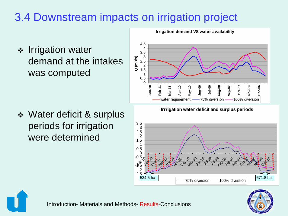
3.4 Downstream impacts on irrigation projectIrrigation demand VS water availability

00.5

11.5

22.5

33.5

44.5

Jan-

10

Feb-

11

Mar

-11

Apr

-10

May

-10

Jun-

09

Jul-0

9

Aug

-08

Sep-

07

Oct

-07

Nov

-06

Dec

-06

Q (m

3/s)

water requirement 75% diversion 100% diversion

Irrigation water demand at the intakes was computed

Water deficit & surplus periods for irrigation were determined

Irrrigation water deficit and surplus periods

-2.5-2

-1.5-1

-0.50

0.51

1.52

2.53

3.5

Jan-1

0Ja

n-30

Feb-21

Mar-11

Mar-31

Apr-20

May-10

May-30

Jun-1

9Ju

l-09

Jul-2

9Aug

-18Sep

-07Sep

-27Oct-

17Nov

-06Nov

-26Dec

-16

75% diversion 100% diversion534.5 ha 671.8 ha

Introduction- Materials and Methods- Results-Conclusions

4. Conclusions

Hare watershed had experienced land use/cover dynamics during the past four decades

Model performance assessment verified that the model simulation results are dependable and SWAT can be utilized in similar watersheds

Simulation results illustrated that land use/cover dynamics has had significant impacts on streamflow

at present Hare River only satisfies 15.75% of downstream irrigation water demand

Introduction- Materials and Methods- Results-Conclusions