Impact of Lateral Flow on Surface Water and Energy Budgets over the

Southern Great Plains – A Modeling Study

Zhao Yang1, Maoyi Huang2, Larry Berg1*, Yun Qian1, William I. Gustafson Jr.1, Yuanhao Fang3,

Ying Liu1, Jerome Fast1, Koichi Sakaguchi1, Sheng-Lun Tai1

1. Pacific Northwest National laboratory, Richland, WA, USA, 99354

2. Office of Science and Technology Integration, National Weather Service, National

Oceanic and Atmospheric Administration, Siliver Spring, MD 20910, USA

3. Department of Hydrology and Atmospheric Sciences, University of Arizona, AZ, USA,

85721

*Correspondence to: Zhao Yang (Zhao.Yang@pnnl.gov), Larry Berg (Larry.Berg@pnnl.gov)

Key Points:

Default parameter values in Noah-MP lead to underestimation of latent heat

fluxes and overestimation of soil moisture.

The introduction of lateral flow via WRF-hydro can alleviate the biases in

latent heat fluxes in high-resolution simulations.

It is crucial to address parametric uncertainty in both land surface and routing

schemes for realistic surface flux simulations.

Acc

epte

d A

rtic

le

This article has been accepted for publication and undergone full peer review but has not been throughthe copyediting, typesetting, pagination and proofreading process, which may lead to differences betweenthis version and the Version of Record. Please cite this article as doi: 10.1029/2020JD033659.

This article is protected by copyright. All rights reserved.

Acc

epte

d A

rtic

le

This article is protected by copyright. All rights reserved.

Abstract

As the horizontal grid spacing decreases, treatment of hydrologic processes in land surface

models, such as the lateral flow of surface and subsurface flow, need to be explicitly represented.

Unlike previous studies that mainly focused on the mountainous regions, in this study the offline

WRF-Hydro model is employed to study the impact of lateral flow on soil moisture and energy

fluxes over the relatively flat southern Great Plains (SGP). The vast amount of measurements

over the SGP provide an unique opportunity to assess the model behavior. In addition, newly

developed land surface properties and input forcing are ingested into the model, in an attempt to

reduce uncertainties associated with the initial and boundary forcing and help to identify model

deficiencies. Our results show that the more realistic inputs (parameters, soil types, forcing) lead

to larger underestimation of latent heat flux and dry bias, indicating the existence of model

structural uncertainty (embedded errors) in WRF-Hydro that need to be characterized to inform

future model development efforts. Including lateral flow processes partly mitigates the model

deficiencies in representing hydrologic processes and alleviates the dry bias. In particular, both

surface and subsurface lateral flow increase soil moisture mainly over the lower elevations,

except that subsurface flow also affects soil moisture over steeper terrains. Additional

simulations are performed to assess the effect of routing resolution on model results. When LSM

resolution is high, noticeable differences in soil moisture are produced between different routing

resolutions especially over steep terrain. Whereas when LSM resolution is coarse, differences

between routing resolutions become negligible, especially over flat terrain.

1 Introduction

The emerging demand to obtain predictability for terrestrial ecosystems across landscapes, with

water, energy, and nutrients as drivers of these dynamic systems, requires process-level

understanding at O(1 km) globally, or O(100 m) locally (Wood et al. 2011); this is known as the

so-called hyperresolution scale. These hyperresolution simulations would require extensive

computation costs, which were previously unrealistic but have become increasingly possible.

The advocacy of hyperresolution land surface models (LSMs) calls for the need to realistically

representing hydrologic processes as well as surface hydrologic information such as topography,

vegetation, and soil hydraulic parameters (Wood et al. 2011; Clark et al. 2015; Maxwell et al.

2015; Chaney et al. 2016; Fan et al. 2019). Hyperresolution LSMs face the challenge to represent

hydrologic processes at the hillslope-to-catchment scales (O(~10 m to 10 km)). These hydrologic

processes, i.e., topographic gradient driven processes, such as water or sediment transport from

the ridges to valleys, operate at scales finer than the traditional LSMs (O(10s km)) and need to be

considered when LSMs are used at hyperresolution scales.

Several previous attempts have been made to understand the importance of lateral flow due to

their importance in hydrologic states and land-atmosphere interactions (Maxwell et al. 2015;

Senatore et al. 2015; Arnault et al. 2016; Chaney et al. 2016; Ji et al. 2017; Arnault et al. 2018;

Rummler et al. 2019; Lahmers et al. 2019; Arnault et al. 2019; Zhang et al. 2019; Fan et al. 2019

and references therein). However, these previous studies have primarily focused on the

mountainous regions, however it is still unknown if lateral flow is equally important over the

relatively flat southern Great Plains (SGP). Therefore, one goal of this study is to understand

how lateral flow would affect soil moisture and surface fluxes over the SGP, where extensive

observations are readily available for evaluating model performance (shown later).

Acc

epte

d A

rtic

le

This article is protected by copyright. All rights reserved.

Focusing on the effect of lateral surface and subsurface flow, Maxwell et al. (2015) found that

the physics-based integrated hydrologic model Parflow can reproduce streamflow and water

table depths reasonably well over the majority of the Continental U.S. (CONUS). Chaney et al.

(2016) developed HydroBlocks that accounts for spatial heterogeneity through hydrologic

response units (HRU). These HRUs are defined using cluster analysis based on land cover,

topography, soil, and location. The vertical profiles of each HRU are then updated using the

Noah-MP LSM (Niu et al. 2011) and exchanges between HRUs are controlled by the dynamic

TOPMODEL via a subsurface kinematic wave. Ji et al. (2017) suggested that surface lateral flow

has a significant influence on soil moisture and evapotranspiration (ET) even at coarse

resolutions, and subsurface lateral flow causes drier ridgelines and wetter valleys. Arnault et al.

(2016) found that overland flow clearly increases infiltration and evapotranspiration at the

beginning of the wet season when soil is still dry. Zhang et al. (2019) used the fully coupled

Weather Research and Forecasting (WRF) model with its hydrological extension WRF-Hydro

(Gochis et al. 2018) and reported a redistribution of infiltration excess in the mountainous area.

Such realistic treatments of hydrologic processes in coupled models typically lead to higher soil

moisture content in the root zone, increases the terrestrial water storage and evapotranspiration,

and decreases the total runoff over the mountainous regions.

It is known that the lateral flow is generally more important at finer grid resolution. Previous

studies suggest treating lateral flow at resolutions of 1 km or finer (Gochis and Chen, 2003). This

is due to the fact that typical overland flood waves are at length scales smaller than 1km. At

larger scales, flood wave and micro-topography features that affect it are poorly represented.

Additionally, at coarser resolutions terrain slopes between grid cells are smoothed as resolution

becomes coarser, which means the lateral flow impact is also scale-dependent. Therefore the

impacts of lateral flow on land surface water and energy budgets differ and are dependent on

landscape characteristics of interest, but it is still not clear at what scale the effects of surface and

subsurface lateral flows become non-negligible. Therefore, another goal of this study is to

examine the critical resolution at which the lateral flow becomes non-negligible with WRF-

Hydro over the SGP. To achieve that, we performed sensitivity experiments of different

horizontal routing resolution at various LSM resolutions. The outcome of this analysis could

serve as guidance for future coupled model experiments.

High resolution LSMs will entail an unprecedented demand for high resolution land

characterization data (Wood et al. 2011), such as soil properties, land use, and land cover type,

and vegetation characteristics. An important source of uncertainty in LSMs lies in inaccuracies in

characterizing these land properties. Recently developed remote sensing and field surveys

provide additional sources of land characteristic datasets for vegetation or soil types that may not

be promptly realized by the modeling community. The utilization of these datasets, assuming

they contain less uncertainty than the old datasets, is therefore important for identifying model

deficiencies and structural errors and guiding future model development.

The representation of soil and vegetation have been found to be a major source of uncertainty in

regional hydrologic simulations (Shi et al. 2014; Osborne et al. 2004; Livneh et al. 2015; De

lannoy et al. 2014). For example, Osborne et al. 2004 found that soil properties could affect the

portioning of surface and subsurface runoff by examining the effects of soil texture. Using two

different soil datasets, Livneh et al. (2015) reported quite different response to extreme events

(floods and droughts). Similarly, the soil hydraulic properties, which are defined depending on

the soil texture of a grid cell following a pre-defined soil parameter table (i.e., SOILPARM), are

Acc

epte

d A

rtic

le

This article is protected by copyright. All rights reserved.

important since they affect water and energy fluxes exchanges within the soil column, and hence

water availability for evapotranspiration. These parameters determine the soil hydraulic

properties and are obtained through field measurements or parameter estimation. In particular,

the default soil parameter table has been developed through the earlier efforts by Cosby et al.

(1984), Chen and Dudhia (2001), NCEP (2012) and Peters-Lidard et al. (1998). For detail

description of the table, readers may refer to Table 1 and 2 in Kishné et al. (2017). These soil

hydraulic parameters are applied both during initializing and running the land surface models,

therefore have far-reaching influence on the outcomes of land surface states in both the coupled

and uncoupled modes (Kishné et al. 2017). The misrepresentation of vegetation is also a source

of uncertainty in the land surface models. Depending on the option chosen, vegetation dynamics

could be treated differently in the land surface models. Kumar et al. (2014) found improvement

in surface heat fluxes and surface temperature and moisture when realistic vegetation parameters

are incorporated into the model. The realistic implementation of satellite-based leaf-area index

(LAI) are also found to reduce temperature biases using different climate models (Knote et al.

2009; Boussetta et al. 2013; Boussetta et al. 2014). Considering the uncertainties associated with

the initial and boundary conditions, the last goal of this study is to evaluate their impacts on soil

moisture and surface fluxes, in an attempt to better simulate the soil moisture and energy fluxes.

By using the most realistic input forcing as possible, this will help to identify model deficiency

and guide future model development.

To summarize, this study will address the following goals related to simulating soil moisture and

energy fluxes over the SGP. Using WRF-Hydro, the first goal is to assess the role of input

forcings in the default Noah-MP LSM. Routing options are turned off at this stage. The second

goal is to understand how surface and subsurface lateral flow would affect soil moisture and

energy respectively. We achieve this by switching on and off the lateral flow options in the

WRF-Hydro model. Finally the third goal is to understand the impact of routing resolution on

soil moisture and energy fluxes over the SGP.

2 Methods

2.1 Model Description

WRF-Hydro was designed as an extensible modeling framework that can host a regional climate

model, a land surface model and a hydrological model. In this study, we focus on evaluating the

offline mode of the model system, without coupling a regional climate model, to quantify

potential issues in land surface representations. The WRF-Hydro hydrological extension includes

a distributed 3-dimensional, variably saturated surface and subsurface flow, channel flow, and a

bucket model to account for baseflow. The lateral surface and subsurface flow are computed on a

separate grid nested within the land surface model grid, which can have a different resolution

than the land surface model. The difference in resolution requires a disaggregation-aggregation

procedure to map land surface hydrological conditions from a “coarse” land surface model grid

to a much more finely resolved terrain routing grid (Gochis and Chen 2003).

Specifically, the disaggregation process is initiated after the LSM process and prior to the routing

of subsurface and surface (Rummler et al. 2019). After the LSM process, the specific hydrologic

variables, such as soil moisture content and infiltration excess, are updated by the LSM and

divided up from the LSM grid into the subgrid cells. Subsurface lateral flow is calculated prior to

the routing of surface flow to allow for exfiltration from fully saturated soil columns to be added

Acc

epte

d A

rtic

le

This article is protected by copyright. All rights reserved.

to the infiltration excess. The subsurface routing scheme was calculated following the method in

Wigmosta et al. (1994) and Wigmosta and Lettenmaier (1999). It calculates a quasi-3-

dimensional flow, which includes the effects of topography, saturated soil depth, and saturated

hydraulic conductivity. Note that lateral subsurface flow only exists in the saturated soil layers

and the hydraulic gradient is calculated based on the slope of the adjacent water table, which is

the depth of the top of the highest saturated layer.

Surface flow is achieved using a fully-unsteady, explicit, finite-difference, diffusive wave

formulation (Julien et al. 1995; Ogden et al. 1997), which can account for backwater effects and

flow on adverse slopes (Senatore et al. 2015). In WRF-Hydro, there are two options available for

surface lateral flow, two-dimensional flow that consider x- and y-dimensional or one

dimensional flow (“D8”) that water flows along the steepest gradient based on total water head

gradient. Overland flow becomes channel inflow if it reaches a channel grid, or it remains as

surface runoff. This study utilizes the steepest gradient method for surface flow. Water flows out

of the bottom soil layer and will go through a groundwater bucket with a fixed capacity; the

baseflow is calculated using an exponential function.

After water is routed through hillslopes along the surface or in the subsurface, through the

groundwater aquifer and channels, state variables such as soil moisture and ponded water on the

routing grid are aggregated back to the native LSM grid using a simple linear average operator.

These updated values are then passed to the next iteration of the LSM timestep.

2.2 Study Area and Observation Data

Our study domain is located over the SGP and covers the spatial extent of 35.2 to 38.0 °N and

95.6 to 99.2 °W (See Fig 1). The spatial domain covers 392 km in both the zonal and meridional

directions. The domain represents a moderate transitional zone with land cover mostly consisting

of cropland and grassland moving from east to west (Koster et al. 2004). The domain-wide

annual average precipitation is approximately 850 mm according to the PRISM data (Daly et al.

2008). It features relatively flat terrain with generally higher elevations on the order of 2100 m to

the west and lower elevations around 300 m to the east. There are local topographic features with

sharp gradients to the southwest of the domain with slopes around 3.5°.

It features extensive observation sites located within the domain, including the US Department of

Energy Atmospheric Research Measurement (ARM) user facility, which contains a number of

extended sites, which provide a unique opportunity as reference datasets. Surface energy fluxes

are available at the ARM sites, collected by using either the eddy correlation (ECOR) or energy

balance Bowen ratio (EBBR) methods (Fig. 1d). Soil moisture and soil type datasets are

available from the Soil Temperature and Moisture Profiles (STAMP) from the ARM sites (Fig.

1d). There are 16 STAMP sites available within the domain. The observation period for STAMP

sites begins in late 2015 and, therefore, model simulated soil moisture are compared to STAMP

sites for 2016 only due to data availability.

Acc

epte

d A

rtic

le

This article is protected by copyright. All rights reserved.

Figure 1: General geophysical features within the research domain. a) terrain height (units: m)

with black box delineating our model domain. b) aspect angle, which is defined as the direction

in which elevation decreases most rapidly, expressed as an azimuth measured clockwise from

north (units: degree). c) slope angle, it is the gradient in the direction in which elevation

decreases most rapidly (units: degree). d) land use and land cover type within the domain.

Circles indicate STAMP locations and crosses indicate locations of EBBR and ECOR stations.

2.3 Input and Forcing Data

The National Land Data Assimilation System phase 2 (NLDAS-2, Xia et al. 2012) is employed

to drive the model. NLDAS-2 is available at 1/8 degree grid spacing. The model is simulated

from 2008 to 2016, the first 3 years are treated as spin-up period. Year 2011-2015 are used for

evaluating latent and sensible heat flux, and 2016 for soil moisture given the availability of

observation datasets. Variables used to force the model include incoming shortwave and

longwave radiation, specific humidity, air temperature, surface pressure, zonal (u) and

meridional (v) components of near surface wind, and precipitation rate. Digital Elevation Map

(DEM) data is obtained from the Hydrological data and maps based on the National

Hydrography Dataset Plus Version 2 (NHDPlusV2, McKay et al. 2012). NHDPlusV2 integrates

the vector stream network, hydrologic unit boundaries with the National Elevation Dataset

(NED) gridded land surface. It also provides stream order and a group of attributes that facilitate

rapid stream network traversal and query. The DEM dataset is processed with the Arcgis toolbox

provided by the WRF-Hydro community to obtain the land surface characteristics that are related

to surface/subsurface routing.

Acc

epte

d A

rtic

le

This article is protected by copyright. All rights reserved.

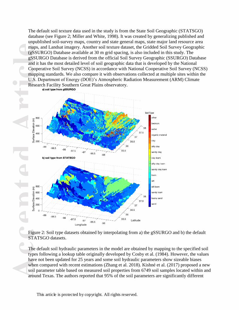
The default soil texture data used in the study is from the State Soil Geographic (STATSGO)

database (see Figure 2; Miller and White, 1998). It was created by generalizing published and

unpublished soil-survey maps, country and state general maps, state major land resource area

maps, and Landsat imagery. Another soil texture dataset, the Gridded Soil Survey Geographic

(gSSURGO) Database available at 30 m grid spacing, is also included in this study. The

gSSURGO Database is derived from the official Soil Survey Geographic (SSURGO) Database

and it has the most detailed level of soil geographic data that is developed by the National

Cooperative Soil Survey (NCSS) in accordance with National Cooperative Soil Survey (NCSS)

mapping standards. We also compare it with observations collected at multiple sites within the

U.S. Department of Energy (DOE)’s Atmospheric Radiation Measurement (ARM) Climate

Research Facility Southern Great Plains observatory.

Figure 2: Soil type datasets obtained by interpolating from a) the gSSURGO and b) the default

STATSGO datasets.

The default soil hydraulic parameters in the model are obtained by mapping to the specified soil

types following a lookup table originally developed by Cosby et al. (1984). However, the values

have not been updated for 25 years and some soil hydraulic parameters show sizeable biases

when compared with recent estimations (Zhang et al. 2018). Kishné et al. (2017) proposed a new

soil parameter table based on measured soil properties from 6749 soil samples located within and

around Texas. The authors reported that 95% of the soil parameters are significantly different

Acc

epte

d A

rtic

le

This article is protected by copyright. All rights reserved.

from the measured values. Sensitivity tests are performed to estimate the uncertainty associated

with using different soil lookup tables in this study. For the values of the updated soil hydraulic

properties, readers are referred to Table 6 in Kishné et al. (2017).

The WRF-Hydro model is run with the default NLDAS-2 precipitation as well as the Stage-IV

precipitation (Du, 2011). The 4-km Stage-IV precipitation were scaled up to a resolution of

0.125° to match NLDAS-2 while preserving grid-mean precipitation and then interpolated to the

grid resolution as input forcing to drive the model. Here we assume that the Stage-IV

precipitation is more accurate given it is able to capture the convective precipitation during the

warm season. In fact, a comparison to gauge precipitation at the SGP central facility reveals that

the Stage-IV precipitation reduces the mean absolute bias by around 4.5% compared to the

NLDAS-2.

2.4 Experiment Design

To elucidate the effect of initial and boundary conditions, the lateral flow process, and resolution

dependence on soil moisture and surface fluxes, we designed several experiments in this study.

Each experiment is based upon the previous experiment to isolate the role played by different

components for how they affect the soil moisture and surface fluxes. The baseline default Noah-

MP (A1) simulation is run with nominal 1 km grid spacing with 392 grid cells in the zonal and

meridional directions. It uses the default tabular values of LAI and maximum vegetation fraction

as a function of land use/land cover, Ball-Berry for canopy stomatal resistance, free drainage for

runoff option, and Monin-Obukohov for surface layer drag coefficient (see Table 1 for more

details). Starting from the default experiment (A1), we replaced the soil with the gSSURGO soil

type in A2. By comparing A1 and A2, we could examine the effect of soil type (e.g., see Table

2). Similarly, the soil parameter lookup table in A2 is updated with the new table developed by

Kishné et al (2017) in A3. By comparing A2 and A3, one may examine the effect of different

soil lookup tables (Table 2).

The default vegetation option in the Noah-MP model uses the maximum Greenness Vegetation

Fraction (GVF) derived from the climatological MODIS mean from 2001–2010 and LAI

interpolated from an empirical lookup table based on land use and land cover type (DVEG=4).

There is also an option available in Noah-MP that uses the actual GVF and LAI (DVEG=7). The

MODIS real-time GVF and LAI observations (MYD15A2H, Myneni et al. 2015) provides a

unique opportunity to feed the model with actual vegetation conditions. The MYD15A2H

products closest to the middle of each month are extracted for the whole simulation period. For

each year, there are 12 sets of GVF and LAI to represent the monthly value. Firstly, these multi-

year monthly GVF and LAI are averaged to obtain a climatological mean for each month. They

are then ingested into A4 to represent the climatological mean vegetation conditions. A5

represents an experiment with near real-time MODIS GVF and LAI. Ideally, A5 is more realistic

in terms of vegetation representation than A3 and A4. By comparing A3 and A4, one could

estimate the effect of using maximum GVF and table-based land cover-dependent LAI versus the

climatological GVF and LAI. By comparing A4 and A5, we could examine the effect of

climatological versus the near real-time GVF and LAI.

On the basis of A5, A6 examines the effect of using Stage-IV precipitation versus the NLDAS-2

default precipitation. A7 and A8 switch on the surface and subsurface flow, respectively, while

A9 turns on both surface and subsurface routing. The surface lateral flow uses the steepest

gradient “D8” method (Table 2). It should be noted that for experiments A1-A6, run without

Acc

epte

d A

rtic

le

This article is protected by copyright. All rights reserved.

lateral flow components, we are actually evaluating the performance of the Noah-MP model. It is

important to note that the results shown later are prone to the underlying assumptions and

uncertainties associated with the Noah-MP. The combinations B1-B5, C1-C5, and D1-D4

examine the effect of routing resolution with LSM grid spacings of 1 km, 4 km, and 10 km,

respectively. Note that at each LSM resolution, we make sure that channel density remains the

same at the preprocessing stage by ensuring that the area of routing grid cells to define stream is

the same across different routing resolutions.

3 Evaluation of WRF-hydro

3.1 Evaluating the impact of input forcings

This section aims to evaluate the effect of different soil type, soil parameter table, vegetation and

precipitation. We emphasize that this study should be considered as a sensitivity study, since we

did not calibrate the WRF-Hydro and our focus is more on evaluating the effect of model inputs

and the routing processes.

3.1.1 Soil texture and soil parameters

The default STATSGO and gSSURGO soil datasets, when interpolated to the model domain at 1

km grid spacing, are shown in Figure 2. The overall spatial pattern of the two datasets agree

reasonably well. The dominant soil types are silt and silt loam, distributed mainly in the southern

and central domain, whereas silty clay loam and clay loam is predominant over the northeastern

part. However, there are also clear differences between these two datasets. The gSSURGO shows

much more detail than the STATSGO. For example, some of the stream networks are clearly

seen in the gSSURGO dataset but are missing in the STATSGO. Inconsistencies exist between

these two datasets, as about 45% of the grid cells are identified differently. Compared to the

STATSGO, the gSSURGO presents a larger percentage of sand, sandy loam, silt loam, and silty

clay loam, and less percentages of loamy sand, loam, clay loam, silty clay, and clay (Figure S1).

The conversion from sand in STATSGO to other soil types in gSSURGO consistently leads to an

increase in LH, resulting in an overall increase of +0.96 Wm-2, whereas the conversion from silt

loam in STATSGO to other soil types in gSSURGO leads to a decrease of -0.65 Wm-2 in LH.

More details on the impact of soil type differences can be seen in Figure S2. Changes in SH is of

the same magnitude but with opposite sign. On average, changing from STATSGO to

gSSURGO leads to about 0.18 Wm-2 increase in SH and decrease in LH.

We have also compared the soil type data collected at the STAMP sites; the gSSURGO is not

superior or more accurate than the STATSGO when compared to the in-situ measurements. Out

of the 16 STAMP stations, both datasets have 6 sites that are consistent with the observed soil

type. We note that this is not an exact fair comparison, since gSSURGO and STATSGO both are

at 1km resolution and represent the dominant soil type within nearest grid cell to the observation,

whereas STAMP represents a point-collected soil sample. Nevertheless, the resulting difference

in soil hydraulic parameters are quite large due to the use of different soil type datasets. The

difference in soil property parameters due to the use of different soil parameter tables is shown in

Figure 3. These changes in soil hydraulic parameters induce changes in soil moisture and surface

energy heat fluxes. Sensitivity tests suggest that maximum soil moisture content (MAXSMC)

and soil conductivity (SATDK) show the strongest control on the energy fluxes, whereas

MAXSMC and wilting point soil moisture (WLTSMC) have the strongest impact for soil

moisture (Figure S3–S5). The results here are consistent with Cuntz et al. (2016), in which the

Acc

epte

d A

rtic

le

This article is protected by copyright. All rights reserved.

authors also identified that MAXSMC and SATDK are the most sensitive parameters that control

the land-atmosphere fluxes exchange and surface runoff.

When the new soil parameter table is used, the simulated soil moisture decreases for loamy sand,

sandy loam, and clay loam, but increases for other soil types, especially for sand and clay (Figure

4a). For the energy fluxes, latent heat fluxes increase for sand and clay, but decrease for other

soil types, of which sandy loam and silty clay loam show the strongest decrease (Figure 4b). The

opposite is true for sensible heat flux, except for loamy sand, of which both latent heat flux and

sensible heat flux decrease (Figure 4c).

Another interesting thing is that even though soil moisture increases for silt loam, loam, silty

clay loam, silty clay, and organic material, LH (SH) decreases (increases) for these soil types.

This is likely because the wilting point of these soil types are higher increased and as a result it is

easier for soil moisture to decline to the wilting point and soil evaporation more easily ceases

being a limit on latent heat flux.

Comparing sand with loam, the sign of changes in soil properties are all the same, except for

SATDK (Figure S6, S7). For SATDK, the positive change of loam and negative change of sand

resulted in decreased LH for loam, but increased LH in sand. This is likely because increased

SATDK allows water to more efficiently exchange water within the soil column and drain it out

the bottom, instead of preserving water within the soil column. Similarly, comparing sand with

silt loam, the only difference is that porosity of silt loam is increased whereas that of sand is

decreased when the new soil parameter table is used (Figure S6, S8), resulting in increased LH in

sand, but decreased LH for silt loam. This suggests that a larger porosity is more likely to

introduce higher LH.

Acc

epte

d A

rtic

le

This article is protected by copyright. All rights reserved.

Figure 3: Differences in soil hydraulic properties induced by using the new soil parameter table

from Kishné et al. (2017), as opposed to the default soil parameter table.

Figure 4: Average difference for each soil type by using the new soil parameter table as opposed

to the default soil parameter table for a) column integrated soil moisture (top 2 m) b) latent heat

flux (LH), and c) sensible heat flux (SH). The error bar indicates one standard deviation.

3.1.2 Comparison to observations

Since different inputs and boundary forcings have been considered in this study; here we try to

compare them within the same context. Figure 5 shows the average monthly time series of LH at

the EBBR and ECOR observation stations with the model values extracted at the nearest grid

cells. The model captures the overall trend of the monthly time series, although it is suggested

that utilizing more realistic data does not ensure better results. This is likely associated with the

model deficiencies, since the default parameters are optimized for global scale simulations (Niu

et al. 2011; Yang et al. 2011). In general, the model underestimates the latent heat flux across all

model experiments, which has been a known issue for land surface models over the Great Plains

(e.g., Lin et al. 2017; Morcrette et al. 2018; Van Weverberg et al. 2018; Zhang et al. 2018; Ma et

al. 2018).

The detail statistics of comparison between the model simulations and the observations, in terms

of model mean bias, root mean square error (RMSE) and Pearson’s correlation coefficient (R)

are shown in Tables S1 and S2 for LH and soil moisture in the Supplementary information. In

general, when compared to observations the differences in error statistics between the suite of

simulations are quite small. One possible reason is that these comparisons are performed only at

a) SM_2m

-0.05

0

0.05

0.1

SM

diff.

[m

]

b) LH

sand

loam

y sa

nd

sand

y lo

am

silt lo

am silt

loam

sand

y clay

loam

silty

clay

loam

clay

loam

sand

y clay

silty

cla

yclay

orga

nic m

ater

ial

wat

er

bedr

ock

othe

r

-5

0

5

10

LH

diff.

(W

m-2

)

c) SH

sand

loam

y sa

nd

sand

y loam

silt loam si

lt

loam

sand

y clay

loam

silty

clay lo

am

clay

loam

sand

y clay

silty

clay

clay

orga

nic m

ater

ial

wat

er

bedr

ock

othe

r

-5

0

5

10

SH

diff. (

W m

-2)

Acc

epte

d A

rtic

le

This article is protected by copyright. All rights reserved.

the ARM sites where observation are available, where the differences are relatively small. There

are other locations in the domain where the differences are significantly larger (shown

later).More specifically, the gSSURGO data shows a nearly negligible effect on the monthly

averaged latent heat flux (Figure 5a); the use of the new soil parameter table slightly reduces the

latent heat flux and leads to a larger underestimation (Figure 5b); the use of the maximum GVF,

although is seemingly unrealistic, in fact produces the best result as compared to the experiments

with realistic MODIS GVF (Figure 5c). Additionally, the use of time-varying GVF and LAI does

not yield significantly different LH than using the climatological GVF/LAI (Figure 5c).

Although Stage-IV precipitation is deemed as more realistic, it leads to larger underestimation of

latent heat flux (Figure 5d). The consideration of lateral flow partly alleviates the

underestimation of LH and slightly improves the performance of LH (Figure 5e). The use of

different routing resolution induces some seasonal differences. Routing resolution only starts to

show an impact below 500 m resolution over the summer months, and above 500 m they are

almost identical when averaged over the ARM sites (Figure 5f).

Figure 5 clearly indicates that the differences induced by different model configurations show

clear distinctions in summer than in other seasons. Figure 6 shows the comparison of soil

moisture to observations collected from the STAMP sites in June, July, and August (JJA) 2016.

Only 2016 is shown because of data availability. Compared to the STAMP sites, all

configurations clearly overestimate soil moisture. Given the underestimation in LH in Figure 5, it

suggests that the Noah-MP needs to evapotranspire more through either direct soil evaporation or

transpiration to simultaneously reduce the biases in soil moisture and latent heat flux.

Specifically, the use of new soil type data and Stage-IV precipitation forcing decrease the bias in

soil moisture while the new soil table and MODIS dynamic vegetation slightly increases the soil

moisture bias. The routing scheme mainly increases soil moisture and, therefore, increases the

soil moisture bias.

Acc

epte

d A

rtic

le

This article is protected by copyright. All rights reserved.

Figure 5: Comparison between monthly mean latent heat flux at the EBBR and ECOR stations

and WRF-Hydro simulation for 2011–2015. Each panel was designed to isolate the effect of a)

soil type dataset of STATSGO (A1) vs. gSSURGO (A2), b) soil parameter table from Cosby et

al. 1984 (A2) vs. from Kishné et al. 2017 (A3), c) default dynamic vegetation (A3) vs. MODIS

climatology (A4) vs. MODIS real time (A5) , d) precipitation from NLDAS-2 (A5) vs. Stage-IV

(A6) , e) without lateral flow (A6) vs. with surface and subsurface lateral flow (A9) and, and f)

different routing resolution for later flow.

6 12 18 24 30 36 42 48 54 600

50

100

150L

H (

W m

-2)

a) Soil type

OBS

Default (A1)

gSSURGO (A2)

6 12 18 24 30 36 42 48 54 600

50

100

150b) Soil table

OBS

old SM table (A2)

new SM table (A3)

6 12 18 24 30 36 42 48 54 600

50

100

150

LH

(W

m-2

)

c) Dynamic vegetation

OBS

Default Vegetation (A3)

MODIS climatological (A4)

MODIS time varying (A5)

6 12 18 24 30 36 42 48 54 600

50

100

150d) Precipitation forcing

OBS

NLDAS-2 prcp (A5)

Stage-IV prcp (A6)

6 12 18 24 30 36 42 48 54 60

Mon

0

50

100

150

LH

(W

m-2

)

e) Routing

OBS

no routing (A6)

routing (A9)

6 12 18 24 30 36 42 48 54 60

Mon

0

50

100

150f) Routing resolution

OBS

100m (B2)

250m (B3)

500m (B4)

1000m (B5)

Acc

epte

d A

rtic

le

This article is protected by copyright. All rights reserved.

Figure 6: Comparison of soil moisture at 5 cm depth between STAMP stations and WRF-Hydro

simulations for June-July-August in 2016. Each panel is similar to Figure 5 but for soil moisture.

3.2 Effects of routing

Figure 7 shows the spatial pattern of soil moisture differences induced by using different routing

options, including no routing (A6), surface routing only (A7), subsurface routing only (A8) and

both surface and subsurface routing (A9). The difference fields thus can isolate the effect of

surface versus subsurface lateral flow and their interaction as simulated by the WRF-Hydro

model. Note these experiments are simulated at 1-km LSM and 250-m routing grid spacing.

Including surface lateral flow consistently increases soil moisture across the soil column, but

mostly only over the lower-elevation convergence regions. For steeper terrain in the southwest of

the domain, surface flow does not show noticeable impact on soil moisture (Figure 7a, 7d, 7g, &

7j). This is because surface lateral flow very efficiently redistributes water from the steep slopes

towards lower elevations. The subsurface lateral flow, besides increasing soil moisture over the

flat terrain at lower elevations, also leads to variable changes in the soil column over the peaks in

the Southwest (Figure 7b, 7e, 7h, & 7k). Soil moisture is increased in the top layers and

decreased in the bottom layers, which is associated with the re-infiltration processes. Over

steeper terrains, lateral flow from the soil column will increase soil moisture content at shallower

layers at the next downstream soil column, while decreasing deep layer soil moisture in the

current soil column. When both surface and subsurface routing are turned on, almost the entire

10 20 30 40 50 60 70 80 900.1

0.15

0.2

0.25

0.3

0.35so

il m

ois

ture

(m

3 m

-3)

a) Soil type

STAMP

Default (A1)

gSSURGO (A2)

10 20 30 40 50 60 70 80 900.1

0.15

0.2

0.25

0.3

0.35b) Soil table

STAMP

old SM table (A2)

new SM table (A3)

10 20 30 40 50 60 70 80 900.1

0.15

0.2

0.25

0.3

0.35

soil

mo

istu

re (

m3 m

-3)

c) Dynamic vegetation

STAMP

Default Vegetation (A3)

MODIS climatological (A4)

MODIS time-varying (A5)

10 20 30 40 50 60 70 80 900.1

0.15

0.2

0.25

0.3

0.35d) Precipitation forcing

STAMP

NLDAS-2 prcp (A5)

Stage-IV prcp (A6)

10 20 30 40 50 60 70 80 90

day

0.1

0.15

0.2

0.25

0.3

0.35

so

il m

ois

ture

(m

3 m

-3)

e) Routing

STAMP

no routing (A6)

surface routing (A7)

subsurface routing (A8)

routing (A9)

10 20 30 40 50 60 70 80 90

day

0.1

0.15

0.2

0.25

0.3

0.35f) Routing resolution

STAMP

100m (B2)

250m (B3)

500m (B4)

1000m (B5)

Acc

epte

d A

rtic

le

This article is protected by copyright. All rights reserved.

domain experiences an increase in the soil moisture content, with the exception of the deeper

layer over the steepest terrain in the southwest (see Figure 7c, 7f, 7i, & 7l). The reduced soil

moisture over the steep terrain is mainly associated with subsurface lateral flow. The response of

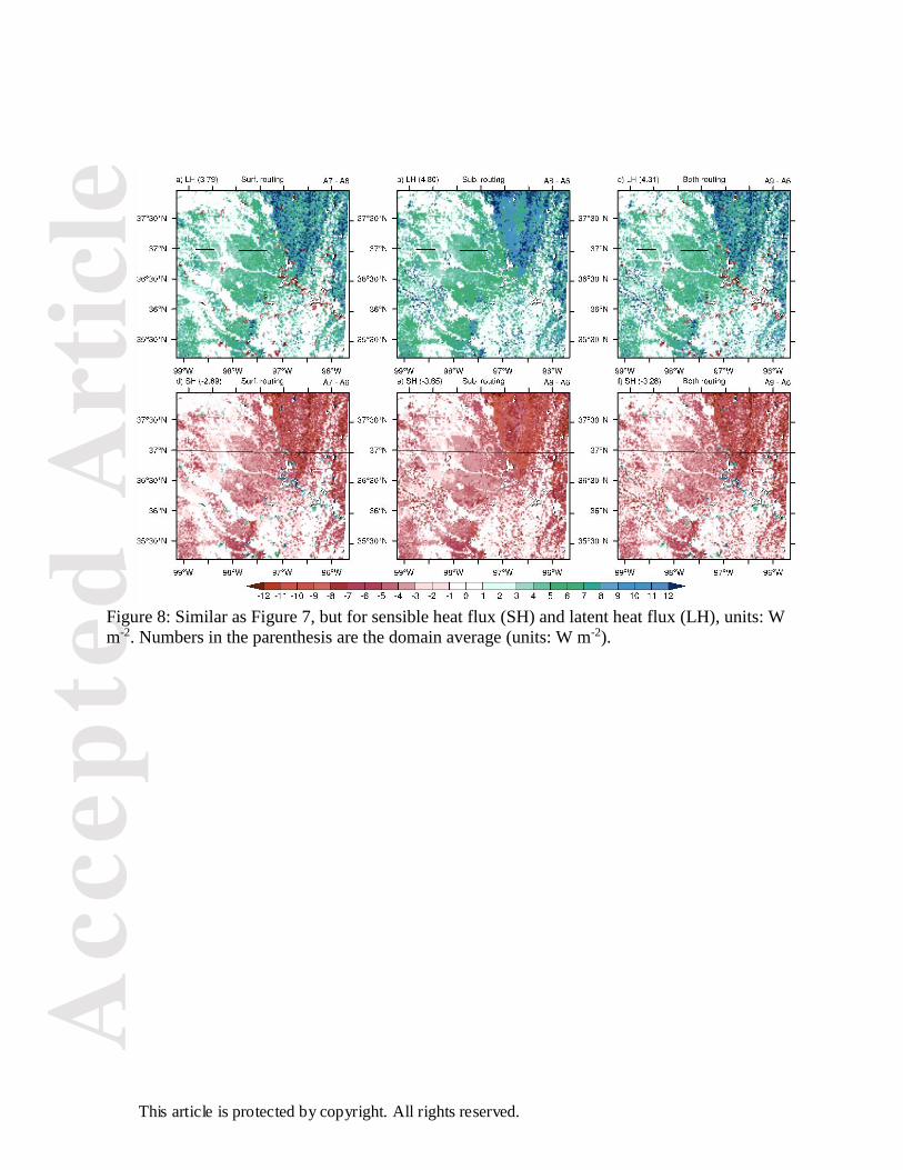
LH and SH to different routing choice is shown in Figure 8. In general, the response of LH

shows a very similar pattern as the soil moisture, while SH shows the opposite.

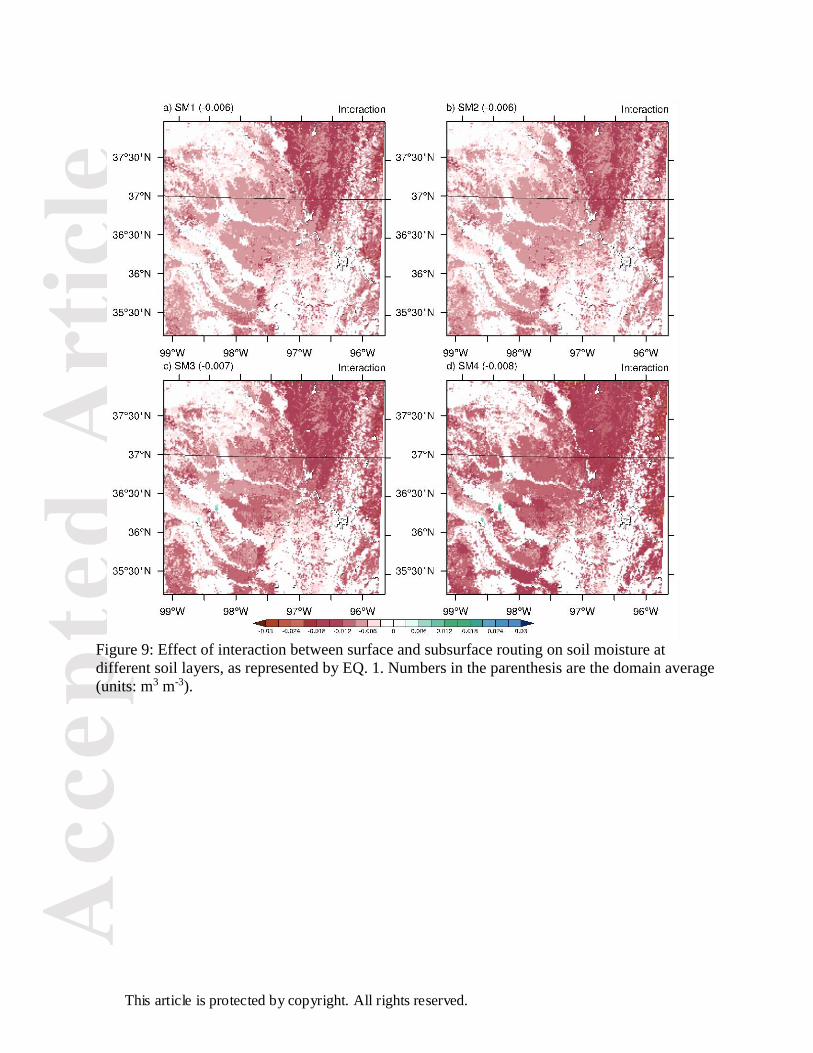
It is interesting to note that the difference between both routing (A9) and subsurface routing only

(A8), which is also often treated as an indication of surface flow effect, has a different pattern

than the difference between surface routing (A7) and no routing (A6) (see difference in 1st and

3rd column in Figure 7). In fact, the difference between simulations with (A7) and without (A6)

surface lateral flow shows the isolated effect of surface lateral flow only, whereas difference

between simulation with both lateral surface and subsurface (A9) and with subsurface routing

only (A8) includes surface effects as well as the interaction between surface and subsurface

lateral flow (see EQ.1 below). The interaction between surface and subsurface routing turns out

to reduce the soil moisture content (Figure 9), meaning that both surface and subsurface lateral

flows are efficiently removing moisture from the soil columns to deep drainage or channel

networks.

𝐼𝑛𝑡𝑒𝑟𝑎𝑐𝑡𝑖𝑜𝑛 = 𝑏𝑜𝑡ℎ 𝑟𝑜𝑢𝑡𝑖𝑛𝑔 − 𝑠𝑢𝑟𝑓𝑎𝑐𝑒 𝑟𝑜𝑢𝑡𝑖𝑛𝑔 − 𝑠𝑢𝑏𝑠𝑢𝑟𝑓𝑎𝑐𝑒 𝑟𝑜𝑢𝑡𝑖𝑛𝑔 + 𝑛𝑜 𝑟𝑜𝑢𝑡𝑖𝑛𝑔 EQ. 1

Acc

epte

d A

rtic

le

This article is protected by copyright. All rights reserved.

Figure 7: Annual averaged soil moisture difference induced by different routing choices. a, d, g,

& j) difference in soil moisture between surface routing (A7) and no routing (A6) in different

soil layers. b, e, h, & k) difference between subsurface routing (A8) and no routing (A6). c, f, i,

& l) difference between both surface and subsurface routing only (A9) and no routing (A6).

Numbers in the parenthesis are the domain average (units: m3 m-3).

Acc

epte

d A

rtic

le

This article is protected by copyright. All rights reserved.

Figure 8: Similar as Figure 7, but for sensible heat flux (SH) and latent heat flux (LH), units: W

m-2. Numbers in the parenthesis are the domain average (units: W m-2).

Acc

epte

d A

rtic

le

This article is protected by copyright. All rights reserved.

Figure 9: Effect of interaction between surface and subsurface routing on soil moisture at

different soil layers, as represented by EQ. 1. Numbers in the parenthesis are the domain average

(units: m3 m-3).

Acc

epte

d A

rtic

le

This article is protected by copyright. All rights reserved.

3.3 Effects of land surface and routing resolution

This section aims to address the question of how land surface variables react to the resolutions of

LSM and routing schemes. WRF-Hydro is designed such that the resolutions of LSM and routing

schemes can be different by using the disaggregation-aggregation methodology. Before the

routing starts, the surface variables from the LSM are disaggregated to the routing grid cells, and

then aggregated to the LSM grid cells when then routing scheme finishes. To test the impact of

resolution, land surface grid spacing is chosen at 1 km, 4 km, and 10 km, while routing grid

spacing is chosen at 100 m, 250 m, 500 m, and 1000 m. Experiments are performed with each

pair of LSM and routing resolution listed above, with the exception of LSM at 10 km and routing

grid spacing at 100 m.

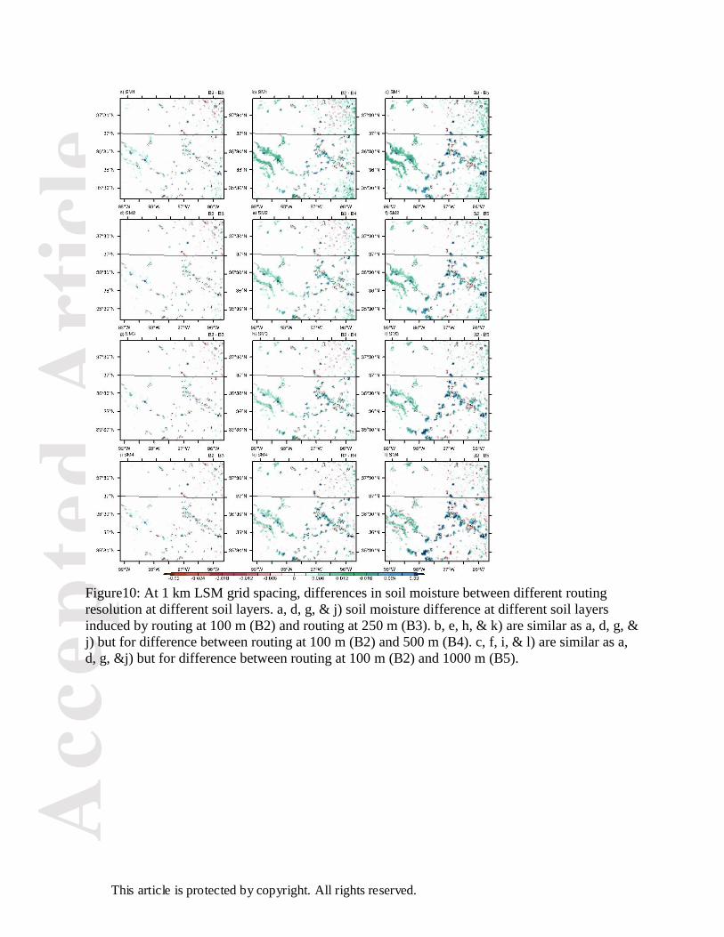
Figure 10 shows the difference in soil moisture due to the change in routing grid spacing when

LSM grid spacing is at 1 km. Overall, there are consistently higher soil moisture contents over

the steep terrain when higher routing resolution is used. The difference fields are consistent for

all four soil layers with a similar magnitude. When a coarser routing resolution is used for

routing, soil moisture is smaller than in simulations with higher routing resolution, indicating

that routing resolution is important in regulating the simulated soil moisture content, with higher

routing resolution leading to larger soil moisture content, especially over steeper terrains.

A similar transition in the difference fields is also found when the LSM grid spacing is coarser at

4 km and 10 km, except that the difference field is almost negligible between routing at 100 m

and 250 m when LSM grid spacing is 4 km, and between 250 m and 500 m when LSM grid

spacing is 10 km (see Figures 11 and 12), meaning that routing does not add extra value at 100 m

(250 m) grid spacing for 4 km (10 km) LSM grid spacing, although the computation cost for

routing is roughly about ~10 times that of routing at 250 m (500 m). Since the difference only

shows for steeper terrain, it suggests that the slope of the terrain is an important factor

controlling the changes in soil moisture induced by routing resolution. Figure 13 presents the

relationship between routing induced soil moisture difference and the slopes at different LSM

resolutions. Some general conclusions are synthesized as follows.

a) At the same LSM resolution, soil moisture generally decreases with a coarser routing

resolution especially over the steeper regions. Or in other words, the difference between the

finest and coarsest routing resolutions always displays the largest difference.

b) soil moisture difference induced by routing resolution over the steep terrain is more obvious in

the shallow soil layers, and this discrepancy is more obvious when LSM resolution is higher.

c) soil moisture is less sensitive to the chosen routing resolution when LSM resolution is coarser,

i.e, when LSM resolution is coarser, the difference in soil moisture due to different routing

resolution gradually fades out.

Acc

epte

d A

rtic

le

This article is protected by copyright. All rights reserved.

Figure10: At 1 km LSM grid spacing, differences in soil moisture between different routing

resolution at different soil layers. a, d, g, & j) soil moisture difference at different soil layers

induced by routing at 100 m (B2) and routing at 250 m (B3). b, e, h, & k) are similar as a, d, g, &

j) but for difference between routing at 100 m (B2) and 500 m (B4). c, f, i, & l) are similar as a,

d, g, &j) but for difference between routing at 100 m (B2) and 1000 m (B5).

Acc

epte

d A

rtic

le

This article is protected by copyright. All rights reserved.

Figure 11: Similar as Figure10, but for LSM resolution at 4 km.

Acc

epte

d A

rtic

le

This article is protected by copyright. All rights reserved.

Figure 12: Similar as Figure 10, but for LSM resolution at 10 km.

Acc

epte

d A

rtic

le

This article is protected by copyright. All rights reserved.

Figure 13: Soil moisture difference between different routing resolutions, as a function of slope.

a-d) for LSM at 1km, e-h) for LSM at 4km and i-l) for LSM at 10km.

The calculation of water balance following Thornthwaite (1948) and Mather (1978) helps to

illustrate the reason why differences are shown between high and low resolution routing. The

water balance equation is as follows:

𝑃 = 𝐸𝑇 + ∆𝑆𝑀 + 𝑆𝑝𝑙𝑢𝑠 EQ2

where P is precipitation (mm), ET is evapotranspiration (mm), ∆𝑆𝑀 is the change in soil water

content (mm); and Splus is water surplus. Because there only exists a short lag between the

generation of surplus water from precipitation and the resultant streamflow, the water surplus can

also be seen as a proxy for runoff (Xue et al. 2018). Figure14 shows the differences in water

balance components for simulations with LSM resolution at 1 km (B2-B5) for JJA 2015. Note

that patterns shown in Figure 14 are the differences between the high and low resolution routing.

Precipitation is the same in these experiments, so it is not shown. Figure 14a-14c indicates that

there is less soil moisture storage change induced in the high-resolution routing. Since soil

moisture is gradually decreasing during the JJA months, suggesting that there is overall more soil

moisture in the high resolution routing, which is consistent with Figure 10. Because of the

presence of more soil moisture over the domain, ET is also more in the high-resolution routing

(Fig 14d-14f). Based on the water balance equation (EQ 2), Figure 14g-14i show the difference

in Surplus, which can be viewed as the amount of water turned into streamflow in the channel, as

explained earlier. It suggests that there is less water converted into streamflow in the high-

resolution routing than in the low-resolution routing, which can be attributed to the generation of

surface runoff (Fig 14j-14l). Note the similarity in spatial pattern between surface runoff and

Acc

epte

d A

rtic

le

This article is protected by copyright. All rights reserved.

Surplus. There is more overland surface runoff when routing at high resolution. The amount of

overland surface runoff originates as infiltration excess, which is a function of precipitation,

existing water head, and infiltration capacity. When calculating lateral surface flow, the effect of

terrain slope is taken into account as part of the friction slope. With high routing resolution, the

terrain effect is more obvious as terrain slope is not smoothed out as in low-resolution routing.

Under the same condition, in high-resolution routing there will be more surface runoff generated

and converged toward lower elevations, and because surface runoff will keep existing on the

land surface, unlike being removed after each time step in the default Noah-MP, the existing

surface runoff will remain in the domain and keep recharging the shallower soil layers, thus

increasing ET. This explains the soil moisture and ET differences shown in Figure 10 and Figure

14d-14f. From a water balance perspective, more surface runoff in the high-resolution routing

results in less subsurface runoff; this explains the opposite pattern in subsurface runoff seen in

Figure 14m-14o. Similar results are found (not shown) for LSM grid spacings of 4 km (C1-C5)

and 10 km (D1-D4).

Acc

epte

d A

rtic

le

This article is protected by copyright. All rights reserved.

Figure 14: Routing-resolution induced differences in water budget components and surface and

subsurface runoff. Difference in soil moisture storage term (∆SM) induced by high and low

routing resolution a) between routing at 100 m and routing at 250 m, b) between routing 100 m

and routing at 500 m, c) between routing 100 m and routing at 1000 m. d-f) are the same as a-c)

but for evapotranspiration (ET). g-i) are the same as d-f) but for Surplus water. j-l) are the same

as d-f) but for surface runoff. m-o) are the same as d-f) but for subsurface runoff.

4 Discussion

WRF-Hydro still underestimates latent heat fluxes over the southern Great Plains, even when

more realistic inputs and boundary forcings are included. As a result, more energy is partitioned

into SH, resulting in a warm bias that is a well-known issue in the modeling community. Many

Acc

epte

d A

rtic

le

This article is protected by copyright. All rights reserved.

studies have attempted to address it from different perspectives (Lin et al. 2017; Ma et al. 2018;

Van Weverberg et al. 2018; Zhang et al. 2018) and different theories are proposed. For example,

an underestimation in evaporative fraction (EF, defined as the ratio of LH to the sum of LH and

SH) has been attributed as the dominant source of error in models with a large warming bias.

Handling of anthropogenic impacts (or lack thereof), such as neglecting irrigation in the LSMs,

has also been attributed to the warming bias (Pei et al. 2016; Yang et al. 2019; Qian et al. 2020).

Here, we show that increased LH and decreased SH occur when lateral flow is considered,

suggesting that lateral flow might also play an important role in alleviating the warming bias

over the SGP.

Comparing simulations using the STATSGO and gSSURGO soil datasets, we found that

differences in soil hydraulic parameters are quite large and lead to changes in domain-averaged

surface energy fluxes and soil moisture. The use of different soil parameter tables gives us the

opportunity to identify which soil parameters are the most sensitive ones to control the rate of

energy fluxes and soil moisture. As shown earlier, MAXSMC and SATDK show the strongest

control on energy fluxes and MAXSMC and WLTSMC have the strongest impact for soil

moisture, which agrees with previous sensitivity studies such as in Cuntz et al. (2016) and Cai et

al. (2014).

We note that the baseline Noah-MP model tends to overestimate soil moisture and underestimate

LH, which indicates more water should be evaporated into the atmosphere instead of retaining in

the soil layers. This bias could potentially be addressed by adjusting parameters suggested in

previous parameter sensitivity studies (e.g. Hogue et al., 2006; Cai et al. 2014; Cuntz et al.

2016). For example, the surface dryness factor, which is defined to determine the soil surface

resistance to ground evapotranspiration, will increase the soil evaporation as it increases.

Similarly, increases in evapotranspiration can also be achieved by lowering the stomatal

resistance (rsmin or rcmin) as it determines the diffusion of water from inside the leaf to the

atmosphere. Another option is to increase roughness length, as it will affect the intensity of

mechanical turbulence and fluxes above the surface. A larger roughness implies more exchange

between the surface and the atmosphere. Calibrating these parameters can improve the model

performance. However, as stated earlier, the purpose of this study is not on parameter calibration

or estimation, but rather on understanding the sensitivity by using different sources of input

forcings.

It is also worth stating that LSMs like Noah-MP were originally developed for simulations with

much coarser grid spacings (e.g,. ~25 km). Some assumptions and parameters used in these

models need to be revisited when running at higher resolutions. For instance, Fmax is the

potential or maximum saturated fraction for a grid cell that was initially derived following the

TOPMODEL concepts rooted from watershed hydrology. When high-resolution digital elevation

models (DEMs) are available, Fmax can be estimated from the distribution function of a

logarithmic topographic index that varies spatially and is resolution-dependent (Niu et al. 2011),

while in typical coarse resolution applications, it is often set universally as 0.38 for convenience.

Another example is the maximum subsurface runoff Rsb,max which should also be spatially

varying and resolution dependent but has been set at 5.0x10-4 mm s-1 based on calibration against

the global runoff field (Niu et al. 2011). When running at higher resolutions, these hard coded

parameters will likely need to be revisited.

We also found that if another soil reference dataset is used, i.e., the soil water and temperature

system (SWATS), the simulated soil moisture is consistently underestimated. The reason we use

Acc

epte

d A

rtic

le

This article is protected by copyright. All rights reserved.

STAMP instead of SWATS is because STAMP soil moisture is deemed as significantly more

reliable than the SWATS (Jenni Kyrouac, personal communication, 2020). Therefore, we

recommend taking precautions when choosing reference datasets since they also contain

uncertainties that could lead to opposite conclusions.

It is interesting to see that both lateral surface and subsurface flow contribute to increased soil

moisture over the SGP. From the water balance perspective, when lateral flow is not turned on,

surface runoff is generated when the effective precipitation exceeds the maximum infiltration

capacity of the underlying soil column. The calculated surface runoff is then accumulated and

removed from the model hydrological budget. At the next time step, the sum of precipitation rate

and existing ponded water head needs to be greater than infiltration capacity again to be able to

generate surface runoff. Conversely, when lateral flows are considered, effective precipitation is

more likely to accumulate on the grid cell given the existence of ponded water, as long as the

sum of precipitation rate and existing ponded water is greater than the infiltration capacity.

Therefore, when surface lateral flow is turned on, it is more likely to generate and maintain

runoff on the surface. The infiltration excess or ponded water later moves freely in the presence

of a hydraulic gradient and infiltrates into the soil column, thereby increasing soil moisture over

the domain.

Since the lateral flow process involves the disaggregation-aggregation and routing of surface and

subsurface flows, computation costs are significantly increased in the offline WRF-Hydro

simulations when lateral flow is turned on. We find that with finer LSM resolution (at 1 km), soil

moisture is more sensitive to the choice of routing resolution, especially over steeper terrains.

This may shed light on the choice of LSM and routing resolution at different topographic

conditions. For example, for complex terrain one may benefit from high LSM and routing

resolution and conversely, over flat regions high resolution routing may be not necessary,

especially when LSM resolution is coarse. One could take advantage of this and design

optimized, multi-resolution model grids that only employ high resolution for the LSM and

routing where there are larger benefits.

5 Conclusions

Using WRF-Hydro, we performed a series of experiments to study the effect of lateral flow on

soil moisture and surface energy fluxes over the SGP. To ensure the correctness of input forcing,

gSSURGO soil dataset, a new soil parameter table, MODIS dynamic vegetation, and Stage-IV

precipitation are ingested into the model for the purpose of minimizing uncertainties associated

with input forcing, where possible. By switching on and off lateral flow options, and testing

different combinations of routing and LSM resolution in the WRF-Hydro, a series of tests were

performed to understand their impact on the soil moisture and surface energy fluxes. We

summarize our key findings as follows.

When compared with observations collected at the STAMP sites, the newly

developed gSSURGO is found to perform identically as the default STATSGO

soil dataset, as both soil datasets extracted at the nearest grid cells have 6 out of

16 sites that have the same soil type as the STAMP.

The default Noah-MP underestimates latent heat fluxes and overestimates soil

moisture when compared with observations collected at the ARM sites. Ingesting

the updated realistic input forcing does not reduce these biases, which indicates

Acc

epte

d A

rtic

le

This article is protected by copyright. All rights reserved.

there are deficiencies embedded in the model. Parameter calibration could

potentially alleviate such deficiencies (Fersch et al. 2020), but the trend towards

higher-resolution modelling primarily suggests to enhance model correspondence

to physical reality by representing new processes such as lateral flow in this study,

or other processes such as groundwater-surface water interaction, rooting

dynamics, and/or irrigation in the model.

The impact of surface and subsurface lateral flow on soil moisture behaves

differently. Surface lateral flow is more likely to increase soil moisture over the

lower terrain and convergence zones, without affecting soil moisture over steeper

terrain. This is likely induced by the efficient redistribution of water from high to

low elevation. The subsurface lateral flow also exhibits an increase in soil

moisture over the entire domain, but with a stronger signal over the steep terrain.

Subsurface lateral flow increases soil moisture in shallower layers but decreases

soil moisture in the deeper layers because of the re-infiltration process, i.e., with a

sufficiently strong topographic gradient, deep-layer soil moisture is transported to

shallower layers at the next downstream grid cells, resulting in the opposite

response of soil moisture in the soil column.

Routing resolution is found to be an important regulator to the response of soil

moisture. With high LSM resolutions, the response of soil moisture is very

sensitive to the choice of routing resolution and higher soil moisture is seen with

finer routing resolution, especially over the steep terrain. With lower LSM

resolution, the added value of using high-resolution routing becomes smaller, e.g.,

the difference between routing at 100 and 250 m spacing when LSM grid spacing

is 4 km, between routing at 250 m and 500 m spacing when LSM grid spacing 10

km, are almost negligible. This indicates that as LSM resolution get coarser, it is

not necessary to use high routing resolution. This indicates that as LSM

resolutions get finer, it is necessary to refine routing representations and better

estimate their parameters. Such studies are becoming more critical as weather and

climate models are moving into higher and higher resolutions.

The present study focuses primarily on the response of soil moisture and energy fluxes to

different input forcing, lateral flow, and LSM and routing resolution. We acknowledge that the

calibration of the parameters associated with generating runoff (Yucel et al. 2015; Zhang et al.

2019; Lahmers et al. 2019; Lahmers et al. 2020; Fersch et al. 2020) is important to ensure

reasonable streamflow predictions. It should be noted that the goal of this study is not to calibrate

the WRF-Hydro model or obtain a best model configuration with smallest model bias. Instead,

our objectives are to quantify the impact of model input, including soil types and properties,

precipitation, vegetation and routing processes on simulation results, and to improve our process-

level understanding of hydrology in this region. The differences induced by different resolution

also calls attention to scale awareness in future development of the routing scheme.

Acknowledgments, Samples, and Data

This research was supported by the Office of Science of the U.S. Department of Energy (DOE)

as part of the Atmospheric System Research (ASR) Program via grant KP1701000/57131. The

research used computational resources from PNNL Research Computing. The Pacific Northwest

Acc

epte

d A

rtic

le

This article is protected by copyright. All rights reserved.

National Laboratory is operated for DOE by Battelle Memorial Institute under Contract DE‐A06‐ 76RLO 1830. We appreciate constructive comments that help to improve the manuscript

from the anonymous reviewers. The WRF-Hydro was downloaded from the NCAR Research

Application Laboratory website (https://ral.ucar.edu/projects/wrf_hydro/model-code). The

ArcGIS toolbox for preprocessing the DEM data was accessed at:

https://ral.ucar.edu/projects/wrf_hydro/pre-processing-tools. We thank the developers for

providing the NLDAS-2, Stage-IV and ARM observations. The authors declare no conflict of

interests. All the scripts for generating the figures are available at Zenodo

http://doi.org/10.5281/zenodo.4521316.

References

Arnault, J., S. Wagner, T. Rummler, B. Fersch, J. Bliefernicht, S. Andresen, and H. Kunstmann

(2016), Role of Runoff–Infiltration Partitioning and Resolved Overland Flow on Land–

Atmosphere Feedbacks: A Case Study with the WRF-Hydro Coupled Modeling System

for West Africa, J. Hydrometeor, 17(5), 1489–1516, doi:10.1175/JHM-D-15-0089.1.

Arnault, J., T. Rummler, F. Baur, S. Lerch, S. Wagner, B. Fersch, Z. Zhang, N. Kerandi, C. Keil,

and H. Kunstmann (2018), Precipitation Sensitivity to the Uncertainty of Terrestrial

Water Flow in WRF-Hydro: An Ensemble Analysis for Central Europe, J. Hydrometeor,

19(6), 1007–1025, doi:10.1175/JHM-D-17-0042.1.

Arnault, J., J. Wei, T. Rummler, B. Fersch, Z. Zhang, G. Jung, S. Wagner, and H. Kunstmann

(2019), A Joint Soil‐ Vegetation‐ Atmospheric Water Tagging Procedure With WRF‐Hydro: Implementation and Application to the Case of Precipitation Partitioning in the

Upper Danube River Basin, Water Resour. Res., 55(7), 6217–6243,

doi:10.1029/2019WR024780.

Boussetta S, Balsamo G, Beljaars A, Kral T, Jarlan L (2013) Impact of a satellite-derived leaf

area index monthly climatology in a global numerical weather prediction model. Int J

Remote Sens 34(9-10):3520–3542

Boussetta S, Balsamo G, Dutra E, Beljaars A, Albergel C (2014) Analysis of surface albedo and

leaf area index from satellite observations and their impact on numerical weather

prediction. ECMWF Technical Memoranda 740:5–10

Cai, X., Z.-L. Yang, C. H. David, G.-Y. Niu, and M. Rodell (2014), Hydrological evaluation of

the Noah-MP land surface model for the Mississippi River Basin, J. Geophys. Res.-

Atmos., 119(1), 23–38, doi:10.1002/2013JD020792.

Chaney, N. W., P. Metcalfe, and E. F. Wood (2016), HydroBlocks: a field-scale resolving land

surface model for application over continental extents, Hydrological Processes, 30(20),

3543–3559, doi:10.1002/hyp.10891.

Chen, F., and J. Dudhia (2001), Coupling an advanced land surface-hydrology model with the

Penn State-NCAR MM5 modeling system. Part I: Model implementation and sensitivity,

Mon. Wea. Rev., 129(4), 569–585, doi:10.1175/1520-

0493(2001)129<0587:CAALSH>2.0.CO;2.

Clark, M. P. et al. (2015), Improving the representation of hydrologic processes in Earth System

Models, Water Resour. Res., 51(8), 5929–5956, doi:10.1002/2015WR017096.

Cosby, B. J., Hornberger, G. M., Clapp, R. B., and Ginn, T. R. (1984), A Statistical Exploration

of the Relationships of Soil Moisture Characteristics to the Physical Properties of Soils,

Water Resour. Res., 20( 6), 682– 690, doi:10.1029/WR020i006p00682.

Acc

epte

d A

rtic

le

This article is protected by copyright. All rights reserved.

Cuntz, M., Mai, J., Samaniego, L., Clark, M., Wulfmeyer, V., Branch, O., Attinger, S., and

Thober, S. (2016), The impact of standard and hard‐ coded parameters on the hydrologic

fluxes in the Noah‐ MP land surface model, J. Geophys. Res. Atmos., 121, 10,676–

10,700, doi:10.1002/2016JD025097.

Daly, C., M. Halbleib, J. I. Smith, W. P. Gibson, M. K. Doggett, G. H. Taylor, J. Curtis, and P.

P. Pasteris (2008), Physiographically sensitive mapping of climatological temperature

and precipitation across the conterminous United States, International Journal of

Climatology, 28(15), 2031–2064, doi:10.1002/joc.1688.

De Lannoy, G. J. M., R. D. Koster, R. H. Reichle, S. P. P. Mahanama, and Q. Liu (2014), An

updated treatment of soil texture and associate hydraulic properties in a global land

modeling system, J. Adv. Model. Earth Syst., 6(4), 957–979,

doi:10.1002/2014MS000330.

Du, J. 2011. GCIP/EOP Surface: Precipitation NCEP/EMC 4KM Gridded Data (GRIB) Stage IV

Data. Version 1.0. UCAR/NCAR - Earth Observing Laboratory.

https://doi.org/10.5065/D6PG1QDD. Accessed 04 Aug 2020.

Fan, Y. et al. (2019), Hillslope Hydrology in Global Change Research and Earth System

Modeling, Water Resour. Res., 55(2), 1737–1772, doi:10.1029/2018WR023903.

Fersch, B., A. Senatore, B. Adler, J. Arnault, M. Mauder, K. Schneider, I. Völksch, and H.

Kunstmann (2020), High-resolution fully coupled atmospheric–hydrological modeling: a

cross-compartment regional water and energy cycle evaluation, Hydrol. Earth Syst. Sci.,

24(5), 2457–2481, doi:10.5194/hess-24-2457-2020.

Gochis, D.J. and F. Chen, 2003: Hydrological enhancements to the community Noah land

surface model. NCAR Technical Note, NCAR/TN-454+STR, 68 pgs. [Available

online: http://www.ucar.edu/communications/technotes/

Gochis, D.J., M. Barlage, A. Dugger, K. FitzGerald, L. Karsten, M. McAllister, J. McCreight, J.

Mills, A. RafieeiNasab, L. Read, K. Sampson, D. Yates, W. Yu, (2018). The WRF-

Hydro modeling system technical description, (Version 5.0). NCAR Technical Note. 107

pages. Available online at https://ral.ucar.edu/sites/default/files/public/WRF-

HydroV5TechnicalDesc.... Source Code DOI:10.5065/D6J38RBJ

Hogue, T. S., L. A. Bastidas, H. V. Gupta, and S. Sorooshian (2006), Evaluating model

performance and parameter behavior for varying levels of land surface model complexity,

Water Resour. Res., 42(8), doi:10.1029/2005WR004440.

Jenni Kyrouac, (2020), Personal communication.

Ji, P., X. Yuan, and X.-Z. Liang (2017), Do Lateral Flows Matter for the Hyperresolution Land

Surface Modeling? J. Geophys. Res., 122(22), 12,077–12,092,

doi:10.1002/2017JD027366.

Jordan, R. E. (1991). A one‐ dimensional temperature model for a snow cover: Technical

documentation for SNTHERM.89. Hanover, NH: Cold Region Research and Engineering

Laboratory, U.S. Army Corps of Engineers.

Julien, P.Y., B. Saghafian and F.L. Ogden, 1995: Raster-based hydrological modeling of

spatially-varied surface runoff. Water Resour. Bull., AWRA, 31(3), 523-536.

Kishné, A. S., Y. T. Yimam, C. L. S. Morgan, and B. C. Dornblaser (2017), Evaluation and

improvement of the default soil hydraulic parameters for the Noah Land Surface Model,

Geoderma, 285(C), 247–259, doi:10.1016/j.geoderma.2016.09.022.

Knote C, Bonafe G, Di Giuseppe F (2009) Leaf area index specification for use in mesoscale

weather prediction systems. Mon Weather Rev 137(10):3535–3550

Acc

epte

d A

rtic

le

This article is protected by copyright. All rights reserved.

Koster, R. D. et al. (2004), Regions of strong coupling between soil moisture and precipitation,

Science, 305(5687), 1138–1140, doi:10.1126/science.1100217.

Kumar, A., F. Chen, M. Barlage, M. B. Ek, and D. Niyogi (2014), Assessing Impacts of

Integrating MODIS Vegetation Data in the Weather Research and Forecasting (WRF)

Model Coupled to Two Different Canopy-Resistance Approaches, J. Appl. Meteor.

Climatol., 53(6), 1362–1380, doi:10.1175/JAMC-D-13-0247.1.

Lahmers, T. M., H. Gupta, C. L. Castro, D. J. Gochis, D. Yates, A. Dugger, D. Goodrich, and P.

Hazenberg (2019), Enhancing the Structure of the WRF-Hydro Hydrologic Model for

Semiarid Environments, J. Hydrometeor, 20(4), 691–714, doi:10.1175/JHM-D-18-

0064.1.

Lahmers, T. M., C. L. Castro, and P. Hazenberg (2020), Effects of Lateral Flow on the

Convective Environment in a Coupled Hydrometeorological Modeling System in a

Semiarid Environment, J. Hydrometeor, 21(4), 615–642, doi:10.1175/JHM-D-19-0100.1.

Lin, Y., W. Dong, M. Zhang, Y. Xie, W. Xue, J. Huang, and Y. Luo (2017), Causes of model dry

and warm bias over central U.S. and impact on climate projections, Nature

Communications, 8(1), 1–8, doi:10.1038/s41467-017-01040-2.

Livneh, B., R. Kumar, and L. Samaniego (2015), Influence of soil textural properties on

hydrologic fluxes in the Mississippi River basin, Hydrol. Processes, 29(21), 4638–4655,

doi:10.1002/hyp.10601.

Ma, H. Y. et al. (2018), CAUSES: On the Role of Surface Energy Budget Errors to the Warm

Surface Air Temperature Error Over the Central United States, J. Geophys. Res., 123(5),

2888–2909, doi:10.1002/2017JD027194.

Mather, J. R.. The climatic water budget in Environmental Analysis. Free Press: Glencoe, IL,

USA, 1978.

Maxwell, R. M., L. E. Condon, and S. J. Kollet (2015), A high-resolution simulation of

groundwater and surface water over most of the continental US with the integrated

hydrologic model ParFlow v3, Geosci. Model Dev., 8(3), 923–937, doi:10.5194/gmd-8-

923-2015.

McKay, L., Bondelid, T., Dewald, T., Johnston, J., Moore, R., and Rea, A., (2012), NHDPlus

Version 2: User Guide.

Miller, D. A., and R. A. White, 1998: A Conterminous United States Multilayer Soil

Characteristics Dataset for Regional Climate and Hydrology Modeling. Earth Interact., 2,

1–26, https://doi.org/10.1175/1087-3562(1998)002<0001:ACUSMS>2.3.CO;2.

Morcrette, C. J. et al. Introduction to CAUSES: Description of weather and climate models and

their near-surface temperature errors in 5 day hindcasts near the southern Great Plains.

Journal of Geophysical Research: Atmospheres 123, 2655–2683 (2018).

Myneni, R., Knyazikhin, Y., Park, T. (2015). MYD15A2H MODIS/Aqua Leaf Area Index/FPAR

8-Day L4 Global 500m SIN Grid V006 [Data set]. NASA EOSDIS Land Processes

DAAC. Accessed 2020-07-24 from https://doi.org/10.5067/MODIS/MYD15A2H.006

NCEP, (2012). Module SF NOAH-LSM v. 3.4.1. http://www.ral.ucar.edu/research/land/

technology/lsm/noahlsm-v3.4.1/modul sf_noahlsm.F.

Niu, G.-Y. et al. (2011), The community Noah land surface model with multiparameterization

options (Noah-MP): 1. Model description and evaluation with local-scale measurements,

J. Geophys. Res., 116(D12), doi:10.1029/2010JD015139.

Ogden, F.L., 1997: CASC2D Reference Manual. Dept. of Civil and Evniron. Eng. U-37, U.

Connecticut, 106 pp.

Acc

epte

d A

rtic

le

This article is protected by copyright. All rights reserved.

Osborne, T. M., D. M. Lawrence, J. M. Slingo, A. J. Challinor, and T. R. Wheeler (2004),

Influence of vegetation on the local climate and hydrology in the tropics: sensitivity to

soil parameters, Clim Dyn, 23(1), 45–61, doi:10.1007/s00382-004-0421-1.

Pei, L., N. Moore, S. Zhong, A. D. Kendall, Z. Gao, and D. W. Hyndman (2016), Effects of

irrigation on summer precipitation over the United States, J. Climate, 29(10), 3541–3558,

doi:10.1175/JCLI-D-15-0337.1.

Peters-Lidard, C. D., E. Blackburn, X. Liang, and E. F. Wood (1998), The Effect of Soil Thermal

Conductivity Parameterization on Surface Energy Fluxes and Temperatures, J. Atmos.

Sci., 55(7), 1209–1224, doi:10.1175/1520-0469(1998)055<1209:TEOSTC>2.0.CO;2.

Qian et al. (2020), Neglecting irrigation contributes to climate model summertime warm-and-dry

biases in the central United States, npj Climate and Atmospheric Science (accepted).

Rummler, T., J. Arnault, D. Gochis, and H. Kunstmann (2019), Role of Lateral Terrestrial Water

Flow on the Regional Water Cycle in a Complex Terrain Region: Investigation With a

Fully Coupled Model System, J. Geophys. Res.-Atmos., 124(2), 507–529,

doi:10.1029/2018JD029004.

Sakaguchi, K., and Zeng, X. (2009), Effects of soil wetness, plant litter, and under‐ canopy

atmospheric stability on ground evaporation in the Community Land Model (CLM3.5), J.

Geophys. Res., 114, D01107, doi:10.1029/2008JD010834.

Senatore, A., G. Mendicino, D. J. Gochis, W. Yu, D. N. Yates, and H. Kunstmann (2015), Fully

coupled atmosphere-hydrology simulations for the central Mediterranean: Impact of

enhanced hydrological parameterization for short and long time scales, Journal of

Advances in Modeling Earth Systems, 7(4), 1693–1715, doi:10.1002/2015MS000510.

Shi, Y., K. J. Davis, F. Zhang, and C. J. Duffy (2014), Evaluation of the parameter sensitivities

of a coupled land surface hydrologic model at a critical zone observatory, J.

Hydrometeorol., 15(1), 279–299, doi:10.1175/JHM-D-12-0177.1.

Thornthwaite, C. (1948). An Approach toward a Rational Classification of Climate.

Geographical Review, 38(1), 55-94. doi:10.2307/210739

Van Weverberg, K. et al. CAUSES: Attribution of surface radiation biases in NWP and climate

models near the U.S. southern Great Plains. Journal of Geophysical Research:

Atmospheres 123, 3612–3644 (2018).

Wigmosta, M. S., L. W. Vail, and D. P. Lettenmaier (1994), A distributed hydrology-vegetation

model for complex terrain, Water Resour. Res., 30(6), 1665–1679,

doi:10.1029/94WR00436.

Wigmosta, M. S., and D. P. Lettenmaier (1999), A comparison of simplified methods for routing

topographically driven subsurface flow, Water Resour. Res., 35(1), 255–264,

doi:10.1029/1998WR900017.

Wood, E. F. et al. (2011), Hyperresolution global land surface modeling: Meeting a grand

challenge for monitoring Earth's terrestrial water, Water Resour. Res., 47(5), 54–10,

doi:10.1029/2010WR010090.

Xia, Y., et al. (2012), Continental‐ scale water and energy flux analysis and validation for the

North American Land Data Assimilation System project phase 2 (NLDAS‐ 2): 1.

Intercomparison and application of model products, J. Geophys. Res., 117, D03109,

doi:10.1029/2011JD016048.

Xue, Z. G., D. Gochis, W. Yu, B. Keim, R. Rohli, Z. Zang, K. Sampson, A. Dugger, D.

Sathiaraj, and Q. Ge (2018), Modeling Hydroclimatic Change in Southwest Louisiana

Rivers, Water, 10(5), 596–20, doi:10.3390/w10050596.

Acc

epte

d A

rtic

le

This article is protected by copyright. All rights reserved.

Yang, Z. et al. (2019), Irrigation Impact on Water and Energy Cycle During Dry Years Over the

United States Using Convection‐ Permitting WRF and a Dynamical Recycling Model, J.

Geophys. Res., 124(21), 11220–11241, doi:10.1029/2019JD030524.

Yang, Z.-L. et al. (2011), The community Noah land surface model with multiparameterization

options (Noah‐ MP): 2. Evaluation over global river basins, J. Geophys. Res., 116(D12),

4257, doi:10.1029/2010JD015140.

Yucel, I., A. Onen, K. K. Yilmaz, and D. J. Gochis (2015), Calibration and evaluation of a flood

forecasting system: Utility of numerical weather prediction model, data assimilation and

satellite-based rainfall, Journal of Hydrology, 523(C), 49–66,

doi:10.1016/j.jhydrol.2015.01.042.

Zhang, C., S. Xie, S. A. Klein, H.-Y. Ma, S. Tang, K. Van Weverberg, C. J. Morcrette, and J.

Petch (2018), CAUSES: Diagnosis of the Summertime Warm Bias in CMIP5 Climate

Models at the ARM Southern Great Plains Site, J. Geophys. Res., 123(6), 2968–2992,

doi:10.1002/2017JD027200.

Zhang, Y., M. G. Schaap, and Y. Zha (2018), A High‐ Resolution Global Map of Soil Hydraulic

Properties Produced by a Hierarchical Parameterization of a Physically Based Water

Retention Model, Water Resour. Res., 54(12), 9774–9790, doi:10.1029/2018WR023539.

Zhang, Z., J. Arnault, S. Wagner, P. Laux, and H. Kunstmann (2019), Impact of Lateral

Terrestrial Water Flow on Land‐ Atmosphere Interactions in the Heihe River Basin in

China: Fully Coupled Modeling and Precipitation Recycling Analysis, J. Geophys. Res.,

48(5), 28–23, doi:10.1029/2018JD030174.

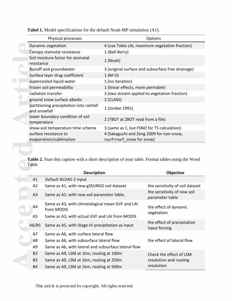
Acc

epte

d A

rtic

le

This article is protected by copyright. All rights reserved.

Tabel 1. Model specifications for the default Noah-MP simulation (A1).

Physical processes Options

Dynamic vegetation 4 (use Table LAI; maximum vegetation fraction)

Canopy stamotal resistance 1 (Ball-Berry)

Soil moisture factor for stomatal resistance

1 (Noah)

Runoff and groundwater 3 (original surface and subsurface free drainage)

Surface layer drag coefficient 1 (M-O)

supercooled liquid water 1 (no iteration)

frozen soil permeability 1 (linear effects, more permable)

radiation transfer 3 (two stream spplied to vegetation fraction)

ground snow surface albedo 2 (CLASS)

partitioning precipitation into rainfall and snowfall

1 (Jordan 1991)

lower boundary condition of soil temperature

2 (TBOT at ZBOT read from a file)

snow-soil temperature time scheme 3 (same as 1, but FSNO for TS calculation)

surface resistance to evaporation/sublimation

4 (Sakaguchi and Zeng 2009 for non-snow, rsurf=rsurf_snow for snow)

Table 2. Start this caption with a short description of your table. Format tables using the Word

Table

Description Objective

A1 Default NLDAS-2 input

A2 Same as A1, with new gSSURGO soil dataset the sensitivity of soil dataset

A3 Same as A2, with new soil parameter table. the sensitivity of new soil parameter table

A4 Same as A3, with climatological mean GVF and LAI from MODIS

the effect of dynamic vegetation

A5 Same as A3, with actual GVF and LAI from MODIS

A6/B1 Same as A5, with Stage-IV precipitation as input the effect of precipitation input forcing

A7 Same as A6, with surface lateral flow

the effect of lateral flow A8 Same as A6, with subsurface lateral flow

A9 Same as A6, with lateral and subsurface lateral flow

B2 Same as A9, LSM at 1km, routing at 100m Check the effect of LSM resolution and routing resolution

B3 Same as A9, LSM at 1km, routing at 250m

B4 Same as A9, LSM at 1km, routing at 500m

Acc

epte

d A

rtic

le

This article is protected by copyright. All rights reserved.

B5 Same as A9, LSM at 1km, routing at 1000m

C1 Same as A6, LSM at 4km, no routing

C2 Same as A9, LSM at 4km, routing at 100m

C3 Same as A9, LSM at 4km, routing at 250m

C4 Same as A9, LSM at 4km, routing at 500m

C5 Same as A9, LSM at 4km, routing at 1000m

D1 Same as A6, LSM at 10km, no routing

D2 Same as A9, LSM at 10km, routing at 250m

D3 Same as A9, LSM at 10km, routing at 500m

D4 Same as A9, LSM at 10km, routing at 1000m

Acc

epte

d A

rtic

le

This article is protected by copyright. All rights reserved.

Figure Caption list:

Figure 1: General geophysical features within the research domain. a) terrain height (units: m)

with black box delineating our model domain. b) aspect angle, which is defined as the direction

in which elevation decreases most rapidly, expressed as an azimuth measured clockwise from

north (units: degree). c) slope angle, it is the gradient in the direction in which elevation

decreases most rapidly (units: degree). d) land use and land cover type within the domain.

Circles indicate STAMP locations and crosses indicate locations of EBBR and ECOR stations.

Figure 2: Soil type datasets obtained by interpolating from a) the gSSURGO and b) the default

STATSGO datasets.

Figure 3: Differences in soil hydraulic properties induced by using the new soil parameter table

from Kishné et al. (2017), as opposed to the default soil parameter table.

Figure 4: Average difference for each soil type by using the new soil parameter table as opposed

to the default soil parameter table for a) column integrated soil moisture (top 2 m) b) latent heat

flux (LH), and c) sensible heat flux (SH). The error bar indicates one standard deviation.

Figure 5: Comparison between monthly mean latent heat flux at the EBBR and ECOR stations

and WRF-Hydro simulation for 2011–2015. Each panel was designed to isolate the effect of a)

soil type dataset of STATSGO (A1) vs. gSSURGO (A2), b) soil parameter table from Cosby et

al. 1984 (A2) vs. from Kishné et al. 2017 (A3), c) default dynamic vegetation (A3) vs. MODIS

climatology (A4) vs. MODIS real time (A5) , d) precipitation from NLDAS-2 (A5) vs. Stage-IV

(A6) , e) without lateral flow (A6) vs. with surface and subsurface lateral flow (A9) and, and f)

different routing resolution for later flow.

Figure 6: Comparison of soil moisture at 5 cm depth between STAMP stations and WRF-Hydro

simulations for June-July-August in 2016. Each panel is similar to Figure 5 but for soil moisture.

Figure 7: Annual averaged soil moisture difference induced by different routing choices. a, d, g,

& j) difference in soil moisture between surface routing (A7) and no routing (A6) in different

soil layers. b, e, h, & k) difference between subsurface routing (A8) and no routing (A6). c, f, i,

& l) difference between both surface and subsurface routing only (A9) and no routing (A6).

Numbers in the parenthesis are the domain average (units: m3 m-3). The black line at 37°N is the

border between Oklahoma and Kansas.

Figure 8: Similar as Figure 7, but for sensible heat flux (SH) and latent heat flux (LH), units: W

m-2. Numbers in the parenthesis are the domain average (units: W m-2).

Figure 9: Effect of interaction between surface and subsurface routing on soil moisture at

different soil layers, as represented by EQ. 1. Numbers in the parenthesis are the domain average

(units: m3 m-3).

Figure10: At 1 km LSM grid spacing, differences in soil moisture between different routing

resolution at different soil layers. a, d, g, & j) soil moisture difference at different soil layers

induced by routing at 100 m (B2) and routing at 250 m (B3). b, e, h, & k) are similar as a, d, g, &

j) but for difference between routing at 100 m (B2) and 500 m (B4). c, f, i, & l) are similar as a,

d, g, &j) but for difference between routing at 100 m (B2) and 1000 m (B5).

Figure 11: Similar as Figure10, but for LSM resolution at 4 km.

Figure 12: Similar as Figure 10, but for LSM resolution at 10 km.

Acc

epte

d A

rtic

le

This article is protected by copyright. All rights reserved.

Figure 13: Soil moisture difference between different routing resolutions, as a function of slope.

a-d) for LSM at 1km, e-h) for LSM at 4km and i-l) for LSM at 10km.

Figure 14: Routing-resolution induced differences in water budget components and surface and

subsurface runoff. Difference in soil moisture storage term (∆SM) induced by high and low

routing resolution a) between routing at 100 m and routing at 250 m, b) between routing 100 m

and routing at 500 m, c) between routing 100 m and routing at 1000 m. d-f) are the same as a-c)

but for evapotranspiration (ET). g-i) are the same as d-f) but for Surplus water. j-l) are the same

as d-f) but for surface runoff. m-o) are the same as d-f) but for subsurface runoff.