IMPACT OF LUMBAR PUNCTURE ON SURVIVAL OF COMATOSE MALAWIANCHILDREN: A PROPENSITY-SCORE-BASED ANALYSIS

By

Jung-Eun Lee

A THESIS

Submitted toMichigan State University

in partial fulfillment of the requirementsfor the degree of

Biostatistics-Master of Science

2016

ABSTRACT

IMPACT OF LUMBAR PUNCTURE ON SURVIVAL OF COMATOSEMALAWIAN CHILDREN: A PROPENSITY-SCORE-BASED ANALYSIS

By

Jung-Eun Lee

Coma is a frequent clinical presentation of severely ill children in sub-Saharan Africa.

It may have a number of infectious and non-infectious etiologies including cerebral malaria,

viral encephalitis, and bacterial and tuberculous meningitis [7]. Due to its high rates of

mortality and morbidity, rapid diagnosis and targeted interventions to optimize outcomes

are critical. However, clinical assessment alone cannot distinguish between these etiologies,

identifying coma etiologies by lumbar puncture (LP) is important.

LP is a clinical procedure that is used to collect and examine the cerebrospinal fluid

surrounding the brain and spinal cord. It has been widely utilized to diagnose symptoms and

signs caused by infection, inflammation, cancer, or bleeding in the central nervous system.

LP is an essential, simple, and widely available, procedure that is generally the only way to

definitively identify underlying infectious coma etiologies. Despite the clear efficacy of LP,

clinicians may be reluctant to perform the procedure in a comatose child, due to concerns

that the procedure may bring out cerebral herniation and death [4].

In this thesis, we aim to assess the impact of LP on the survival of comatose children. We

performed a retrospective cohort study on survival of comatose Malawian pediatric inpatients

recruited over consecutive rainy seasons from 1997-2013. Due to the lack of randomness in

being treated (LP) and untreated (Non-LP) groups, baseline characteristics are not balanced.

We applied propensity score methods to compensate the imbalance. Our analysis results

showed no impact in death rate associated with LP.

ACKNOWLEDGMENTS

First and above all, I praise and thank to the God, the Almighty, for His showers of blessings

throughout my research work and grating me the capability to proceed successfully.

I would like to express my deep and sincere gratitude to my research supervisor, Dr.

Chenxi Li for giving me the opportunity to work on this research topic and providing invalu-

able guidance throughout the research. His vision and motivation have deeply inspired me.

He has taught me the methodology to carry out the research and to present the research

works as clearly as possible. It was a great privilege and honor to work and study under

his guidance. I would also like to thank professor Joseph Gardiner, and professor Zhehui

Luo for serving as my committee members, especially for letting my defense be an enjoyable

moment, and for their brilliant comments and suggestions.

I am extremely thankful to my family for their love, understanding, prayers and continu-

ing support. My special thanks goes to my friends, Sang In Chung, Miran Kim, and Sunnie

Oh for their prayers and love.

iii

TABLE OF CONTENTS

LIST OF TABLES . . . . . . . . . . . . . . . . . . . . . . . . . . . . . . . . . . . . v

LIST OF FIGURES . . . . . . . . . . . . . . . . . . . . . . . . . . . . . . . . . . . vii

Chapter 1 Introduction . . . . . . . . . . . . . . . . . . . . . . . . . . . . . . . 11.1 Cerebral Malaria and Lumbar Puncture . . . . . . . . . . . . . . . . . . . . . 11.2 Survival Data and Survival Analysis . . . . . . . . . . . . . . . . . . . . . . . 3

1.2.1 Lumbar Puncture Data . . . . . . . . . . . . . . . . . . . . . . . . . . 41.2.1.1 Treatments and Outcomes . . . . . . . . . . . . . . . . . . . 51.2.1.2 Characteristic Variables . . . . . . . . . . . . . . . . . . . . 51.2.1.3 Time Variables . . . . . . . . . . . . . . . . . . . . . . . . . 81.2.1.4 Selection Bias . . . . . . . . . . . . . . . . . . . . . . . . . . 8

Chapter 2 Methods . . . . . . . . . . . . . . . . . . . . . . . . . . . . . . . . . . 112.1 Survival Analysis . . . . . . . . . . . . . . . . . . . . . . . . . . . . . . . . . 11

2.1.1 The Hazard Function . . . . . . . . . . . . . . . . . . . . . . . . . . . 122.1.2 Competing Risks . . . . . . . . . . . . . . . . . . . . . . . . . . . . . 142.1.3 Cox Proportional Hazards Model . . . . . . . . . . . . . . . . . . . . 152.1.4 Log-Rank Test . . . . . . . . . . . . . . . . . . . . . . . . . . . . . . 16

2.2 Propensity Score . . . . . . . . . . . . . . . . . . . . . . . . . . . . . . . . . 182.2.1 Inverse Probability of Treatment Weighting . . . . . . . . . . . . . . 192.2.2 Stratification . . . . . . . . . . . . . . . . . . . . . . . . . . . . . . . 20

2.3 SAS Procedures . . . . . . . . . . . . . . . . . . . . . . . . . . . . . . . . . . 20

Chapter 3 Results . . . . . . . . . . . . . . . . . . . . . . . . . . . . . . . . . . . 223.1 Data Exploration . . . . . . . . . . . . . . . . . . . . . . . . . . . . . . . . . 223.2 Propensity Score Estimation . . . . . . . . . . . . . . . . . . . . . . . . . . . 223.3 Impact of LP on In-Hospital Death Rate . . . . . . . . . . . . . . . . . . . . 27

3.3.1 Results from Inverse Probability of Treatment Weighting . . . . . . . 273.3.2 Results from Stratification . . . . . . . . . . . . . . . . . . . . . . . . 303.3.3 Comparison of Death Rates over Different Time Windows . . . . . . 323.3.4 Subgroup Analyses . . . . . . . . . . . . . . . . . . . . . . . . . . . . 35

3.3.4.1 Influence of Papilledema . . . . . . . . . . . . . . . . . . . . 353.3.4.2 Impact of LP on survival of children with increased brain

volume . . . . . . . . . . . . . . . . . . . . . . . . . . . . . 363.3.5 Validation of Assumption . . . . . . . . . . . . . . . . . . . . . . . . 38

Chapter 4 Conclusion and Discussion . . . . . . . . . . . . . . . . . . . . . . 40

BIBLIOGRAPHY . . . . . . . . . . . . . . . . . . . . . . . . . . . . . . . . . . . . 42

iv

LIST OF TABLES

Table 1.1: Descriptions of Categorical Variables from the Original Data. The TotalNumber of subjects in the original data set is 2,399. . . . . . . . . . . . 7

Table 1.2: Descriptions of Continuous Variables from the Original Data. The TotalNumber of subjects in the original data set is 2,399. . . . . . . . . . . . 8

Table 1.3: Distributions of Time to Event. . . . . . . . . . . . . . . . . . . . . . . 8

Table 3.1: Baseline Characteristics of the Children before Propensity Score Adjust-ment (Analysis including Papilledema). . . . . . . . . . . . . . . . . . . 24

Table 3.2: Baseline Characteristics of the Children before Propensity Score Adjust-ment (Analysis excluding Papilledema). . . . . . . . . . . . . . . . . . . 24

Table 3.3: Summary Statistics of Propensity Score in LP and Non-LP groups. Pa-pilledema was included in PS estimation. The number of subjects is1,010. . . . . . . . . . . . . . . . . . . . . . . . . . . . . . . . . . . . . . 25

Table 3.4: Summary Statistics of Propensity Score in LP and Non-LP groups. Pa-pilledema was excluded in PS estimation. The number of subjects is1,772. . . . . . . . . . . . . . . . . . . . . . . . . . . . . . . . . . . . . . 26

Table 3.5: Number of Subjects in Each Stratum. . . . . . . . . . . . . . . . . . . . 32

Table 3.6: Results of Log-Rank Tests for Effect of Treatment over Specific TimeWindows. . . . . . . . . . . . . . . . . . . . . . . . . . . . . . . . . . . 35

Table 3.7: Results of Analysis of Maximum Likelihood Estimates for the IPTW CoxModel Considering the Effect Modification by Papilledema. . . . . . . . 36

Table 3.8: Distributions of LP and Non-LP groups within Positive and NegativePapilledema Groups. . . . . . . . . . . . . . . . . . . . . . . . . . . . . 37

Table 3.9: Distribution of Subjects who have Edema score. . . . . . . . . . . . . . 38

Table 3.10: Results of Analysis of Maximum Likelihood Estimates for the IPTW CoxModel Considering the Effect Modification of Edema. . . . . . . . . . . 38

Table 3.11: Results of Linear Hypotheses Testing Results for Proportionality: Pa-pilledema Subgroup Analysis. . . . . . . . . . . . . . . . . . . . . . . . 39

v

Table 3.12: Results of Linear Hypotheses Testing Results for Proportionality: EdemaSubgroup Analysis. . . . . . . . . . . . . . . . . . . . . . . . . . . . . . 39

vi

LIST OF FIGURES

Figure 1.1: Distributions of Time to Death for LP (LP=1) and Non-LP (LP=0)Groups. . . . . . . . . . . . . . . . . . . . . . . . . . . . . . . . . . . . . 9

Figure 1.2: Distributions of Time to Discharge for LP (LP=1) and Non-LP (LP=0)Groups. . . . . . . . . . . . . . . . . . . . . . . . . . . . . . . . . . . . . 10

Figure 3.1: Study Populations in the LP data set. . . . . . . . . . . . . . . . . . . . 23

Figure 3.2: Distribution of Propensity Score across LP and Non-LP groups. Pa-pilledema information was included in propensity score estimation. . . . 25

Figure 3.3: Distribution of Propensity Score across LP and Non-LP groups. Propen-sity scores were estimated without Papilledema information. . . . . . . 26

Figure 3.4: Comparison of Hazard functions between LP (LP=1) and Non-LP (LP=0)groups. The PS was estimated with Papilledema. The value of the band-width was set with default value. . . . . . . . . . . . . . . . . . . . . . . 28

Figure 3.5: Comparison of Hazard functions between LP (LP=1) and Non-LP (LP=0)groups. The PS was estimated with Papilledema. The value of the band-width was set as 8. . . . . . . . . . . . . . . . . . . . . . . . . . . . . . 28

Figure 3.6: Comparison of Hazard functions between LP (LP=1) and Non-LP (LP=0)groups. The PS was estimated with Papilledema. The value of the band-width was set as 10. . . . . . . . . . . . . . . . . . . . . . . . . . . . . . 29

Figure 3.7: Comparison of Hazard functions between LP (LP=1) and Non-LP (LP=0)groups. The PS was estimated with Papilledema. The value of the band-width was set as 12. . . . . . . . . . . . . . . . . . . . . . . . . . . . . . 29

Figure 3.8: Comparison of Hazard functions between LP (LP=1) and Non-LP (LP=0)groups. The PS was estimated without Papilledema. The value of thebandwidth was set with default value. . . . . . . . . . . . . . . . . . . . 30

Figure 3.9: Comparison of Hazard functions between LP (LP=1) and Non-LP (LP=0)groups. The PS was estimated without Papilledema. The value of thebandwidth was set as 8. . . . . . . . . . . . . . . . . . . . . . . . . . . . 31

vii

Figure 3.10: Comparison of Hazard functions between LP (LP=1) and Non-LP (LP=0)groups. The PS was estimated without Papilledema. The value of thebandwidth was set as 10. . . . . . . . . . . . . . . . . . . . . . . . . . . 31

Figure 3.11: Comparison of Hazard functions between LP (LP=1) and Non-LP (LP=0)groups. The PS was estimated without Papilledema. The value of thebandwidth was set as 12. . . . . . . . . . . . . . . . . . . . . . . . . . . 32

Figure 3.12: Comparison of Cumulative Incidence Functions between LP (LP=1) andNon-LP (LP=0) groups. The PS was estimated with Papilledema. . . . 33

Figure 3.13: Comparison of Cumulative Incidence Functions between LP (LP=1) andNon-LP (LP=0) groups. The PS was estimated without Papilledema. . 34

Figure 3.14: Comparison of Distributions of Time to Death between Positive (PAP=1)and Negative (PAP=0) Papilledema Groups. . . . . . . . . . . . . . . . 36

Figure 3.15: Comparison of Distributions of Time to Discharge between Positive (PAP=1)and Negative (PAP=0) Papilledema Groups. . . . . . . . . . . . . . . . 37

viii

Chapter 1

Introduction

1.1 Cerebral Malaria and Lumbar Puncture

In low and middle-income countries, coma is a frequent clinical presentation of severely ill

children. The most common cause of these comatose patients is cerebral malaria (CM). The

global annual incidence of severe malaria can be estimated at approximately two million

cases and about 90% of the world’s severe and fatal malaria occurs to young children in

sub-Saharan Africa [15].

The World Health Organization (WHO) defines cerebral malaria as a clinical syndrome

characterized of coma (inability to localize a painful stimulus) at least one hour after termi-

nation of a seizure or correction of hypoglycemia, asexual forms of Plasmodium falciparum

parasites on peripheral blood smears, and exclusion of other causes of encephalopathy (e.g.

viral encephalitis, poisoning, and metabolic disease) [10]. However, this definition is not well

observed in practice. Patients whose coma is caused by other encephalopathies or previously

unrecognized neurological abnormalities but have incidental parasitemia may be included.

Due to the lack of specificity, using clinical evaluation by itself cannot differentiate between

these etiologies [18]. By reasons of the amount of risk and the low feasibility of experimen-

tally treating all cases of infectious coma etiologies in suspected children with CM, utilizing

lumbar puncture (LP) increases the chance for correct treatment and accurate diagnoses.

Lumbar puncture (LP) is a clinical procedure that is used to collect and examine the

1

cerebrospinal fluid (CSF) surrounding the brain and spinal cord. It has been widely utilized

to diagnose symptoms and signs caused by infection, inflammation, cancer, or bleeding in

the central nervous system. LP is also used to measure the CSF pressure within the epidural

space [9]. In particular, LP has been a valuable and generally the only available tool for

identifying the etiology of CM. Despite its efficacy, clinicians who lack access to such resources

like pre-procedural neuro-imaging may be hesitant to perform it. This is because performing

LP on comatose patients may incur cerebral herniation and death if the absence of brain shift

or increased intracranial pressure (ICP) is not verified through neuroimaging or molecular

testing [19, 1].

Moxon et al. examined safety of LP in comatose African children with clinical features of

CM [2]. They found no evidence that undergoing LP increases mortality in comatose children

with suspected CM. This was also true in children with magnetic resonance imaging (MRI)

evidence of severe brain swelling. In addition, the study provided evidence that LP does not

play a causal role in fatal herniation in the context of diffusely increased ICP. They conjecture

that LP does not exacerbate herniation in CM because, during LP, the CSF pressure is able

to rapidly equilibrate.

In this study, we extend the Moxon’s work to survival analysis. We conduct statistical

analysis to assess the impact of LP on the death rate of comatose children. In particular,

we examine whether i) the temporal association between LP and death implies causation;

ii) LP contributes to mortality in children with CM who have increased ICP by comparing

the hospital death rates between the treatment and control groups; and iii) effect of LP on

death in CM children with and without Papilledema.

2

1.2 Survival Data and Survival Analysis

Survival data are in the form of time from a well-defined origin until the occurrence of

some particular event or end-point such as death, disease onset, machine failure, automobile

accidents, promotions, or end of marriage [3]. Survival data are not amenable to conventional

statistical procedures because of their special feature, censoring. Censoring is a typical

characteristic in survival analysis, representing a particular type of coarsened data. It occurs

when the end-point of interest has not been observed for a subject due to end of investigation,

drop-out of subjects, or the experiment design with threshold for the time window. The

information of such censored observations is therefore incomplete. In addition, survival data

are also generally not symmetrically distributed but positively skewed [3]. The survival

times usually have specialized non-normal distributions, such as the exponential, Weibull,

and log-normal. Hence, conventional statistical analysis methods are limited for dealing with

survival data.

Unlike conventional statistical methods, survival analysis correctly incorporates infor-

mation from both censored and uncensored observations in estimating important model

parameters. Two key elements of survival data are i) a time to event/censoring indicating

how long until the subject either experienced the event or was censored, and ii) a censoring

indicator denoting whether an observational event was experienced or censored. Based on

the two elements, the survival and hazard functions are estimated for describing the distri-

bution of event times. The survival function represents the probability that an individual

survives (or does not experience the event) beyond any given time. The hazard function

gives the potential risk or hazard of an event at the specified time. It is generally of interest

in survival analysis to describe the relationship of a factor of interest (e.g. treatment) to the

3

time to event, in the presence of several covariates (e.g. age, gender, race, etc.) A number

of models from parametric, nonparametric and semi-parametric approaches are available to

analyze the relationship of a set of predictor variables with the survival time.

In our survival analysis, we examine the death hazard rate between patients with LP,

(i.e. the treatment group) and without LP (i.e. the control group.) Discharge from the

medical institution is regarded as a competing endpoint, which is actually dependent on

time to death. All the survival analyses in this study are therefore for competing risks, i.e.

estimating cause-specific hazard of death.

1.2.1 Lumbar Puncture Data

We conduct a retrospective cohort study of pediatric inpatients recruited from 1997 to 2015

at the Pediatric Research Ward at Queen Elizabeth Central Hospital (QECH) in Blantyre,

Malawi. The study population contains 1, 772 comatose children aged two months to fourteen

years, including 1, 442 patients in the treatment group and 350 patients in the control group.

Patients in the treatment group received LPs in one of two ways. If the patients were directly

admitted to QECH, the procedure was done as part of the admission process. On the other

hand, if patients were referred to QECH from other accident and emergency departments,

the LPs were done at those institutions. LPs were not done in the control group because

clinicians determined that the children were not stable enough to tolerate the procedure.

The dataset at hand is comprised of characteristic variables on the admission to the medical

institution that influenced a clinician’s decision to perform a LP or were independently

associated with death. Several time variables such as time of admission, death, hospital

discharge, and LP operation are also included in the dataset.

4

1.2.1.1 Treatments and Outcomes

The treatment group contains 81.4% and the control group contains 18.6% of comatose

children. The total number of subject is 1, 772. The patients in the control group have not

received LP because of one or more of five reasons below:

1. The clinician was concerned that the child was not stable enough to tolerate an LP

based on shock, severe respiratory distress or intractable seizures.

2. The clinician identified Papilledema on retinal examination.

3. LP was attempted but failed for technical reason(s).

4. The parent did not consent to LP.

5. The child regained consciousness before LP was performed.

For outcome, 3, 6, 12-hour mortality rates and overall mortality rate during hospitaliza-

tion were used to evaluate the treatment effects.

1.2.1.2 Characteristic Variables

The statistical analysis includes factors which affect a physician’s decision to perform LP

and others obtained from previous studies associated with a fatal outcome.

• Depth of coma (Blantyre Coma Score)

• Systolic blood pressure for age

• Weight-for-height z-score (nutritional status)

• Respiratory distress or acidotic breathing

5

• Pulse rate

• Cardiovascular system examination (signs of heart failure)

• Gender

• Admission blood glucose concentration

• Peripheral parasite density

• Hematocrit

• Malaria retinopathy status

• Papilledema

Weight-for-height z-score was created by weight and height according to the WHO Child

Growth Standards [8]. Respiratory distress or acidotic breathing was determined from sign

of grunting, deep breath and normal chest exam: if any of the three is abnormal, then it

suggests that respiratory disease is present. In the data, 256 patients did not have malaria

retinopathy status on admission. As a result we imputed the value of this status utilizing

logistic regression based on: platelet count, hematocrit, and glucose. Where the probability

of retinopathy is greater than 50%, we set this value as positive, if not negative. The

threshold for the probability was set to be consistent with Moxon’s [2]. Papilledema was

considered an important factor for the statistical analysis. However, a significant portion of

children (i.e. 43%) have missing information of Papilledema determination. We therefore

performed sub-analysis without Papilledema for confirming significant role of Papilledema in

statistical analysis. Any subjects with missing data, other than retinopathy or Papilledema,

6

were excluded from the statistical analysis. Tables 1.1 and 1.2 shows explanatory variables

from the original data set and their descriptions.

Table 1.1: Descriptions of Categorical Variables from the Original Data. The Total Numberof subjects in the original data set is 2,399.

Variable Description Units Count

COMASCDepth of comma (Blantyre comascore: ≤ 2 = unrousable coma)

0=Most severe1=Severe2=Less SevereNo. of Missing

383949

1,0670

BPSTAT Systolic blood pressure for age

0=Low1=Normal2=HighNo. of Missing

282,071

89211

WHWeight-for-Height Z-score(Nutritional status)

0=Normal1=LowNo. of Missing

2,067211121

RESPDIS Respiratory distress0=Not Present1=PresentNo. of Missing

1,228821350

PULSESTAT Pulse rate

0=Low1=Normal2=HighNo. of Missing

43925

1,299132

NHEARTCardiovascular system examination(Normal heart test)

0=Normal1=AbnormalNo. of Missing

1352,236

28

SEX Gender0=Male1=FemalNo. of Missing

1,1431,252

4

ADMRETIN Malaria retinopathy status0=Not Present1=PresentNo. of Missing

8221,321256

PAP Papilledema0=Not Present1=PresentNo. of Missing

1,033241

1,125

7

Table 1.2: Descriptions of Continuous Variables from the Original Data. The Total Numberof subjects in the original data set is 2,399.

VariableNo. ofMissing

Description LP Mean SD Min Max

ADMHCT 122 HematocritNon-LP 21.34 8.38 6.00 59.00

LP 23.75 8.07 2.00 46.90

ADMGLUC 10Admission

blood glucoseNon-LP 6.29 3.98 0.5 29.60

LP 6.78 4.05 0.3 33.00

LOGADMPTA 189Peripheral

parasite DensityNon-LP 10.22 3.32 0 14.29

LP 9.22 4.27 0 15.02

1.2.1.3 Time Variables

Several time variables such as times of admission, death and hospital discharge as well as LP

operation are included in the dataset. The time origin is the time of LP performed for the

treatment group or the time of admission for the control group. Time of death is regarded

as the endpoint while discharge from the medical institution is regarded as a competing

endpoint. Table 1.3 compares the distributions of time to event (i.e. death or discharge)

between LP and Non-LP groups. Figures 1.1 and 1.2 show distributions of time to event in

LP and Non-LP groups.

Table 1.3: Distributions of Time to Event.

LP Outcome No. of Subjects Mean SD Min Max

Non-LPDischarge 259 3.555 2.34 0.500 26.79Death 91 0.798 1.38 0.014 11.17

LPDischarge 1206 3.791 2.98 0.208 33.77Death 216 1.411 3.27 0.021 31.11

1.2.1.4 Selection Bias

As we mentioned above, decisions about whether LPs were medically contraindicated were

made by different admitting clinicians, resulting in non-random variation in severity of illness

among children who did and did not received LPs. Due to the lack of randomness in treated

8

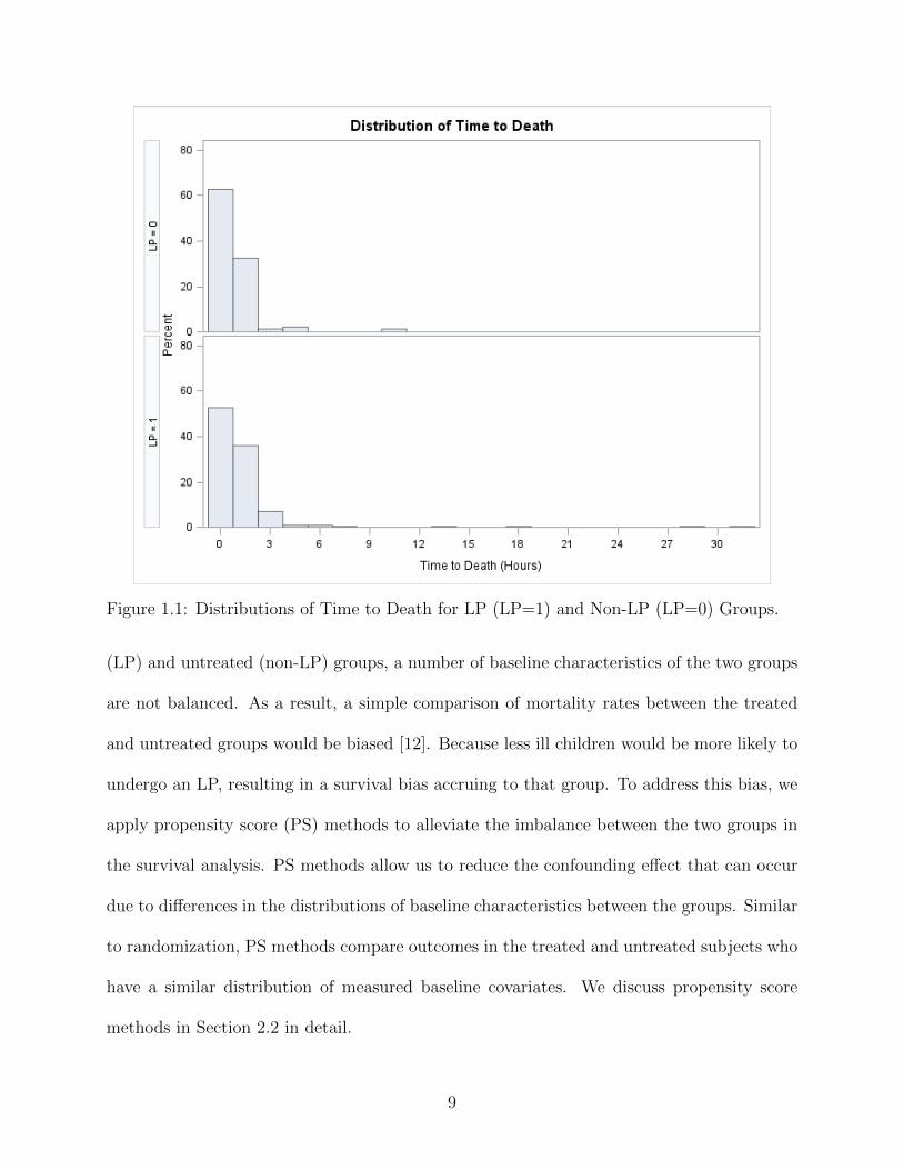
Figure 1.1: Distributions of Time to Death for LP (LP=1) and Non-LP (LP=0) Groups.

(LP) and untreated (non-LP) groups, a number of baseline characteristics of the two groups

are not balanced. As a result, a simple comparison of mortality rates between the treated

and untreated groups would be biased [12]. Because less ill children would be more likely to

undergo an LP, resulting in a survival bias accruing to that group. To address this bias, we

apply propensity score (PS) methods to alleviate the imbalance between the two groups in

the survival analysis. PS methods allow us to reduce the confounding effect that can occur

due to differences in the distributions of baseline characteristics between the groups. Similar

to randomization, PS methods compare outcomes in the treated and untreated subjects who

have a similar distribution of measured baseline covariates. We discuss propensity score

methods in Section 2.2 in detail.

9

Figure 1.2: Distributions of Time to Discharge for LP (LP=1) and Non-LP (LP=0)Groups.

10

Chapter 2

Methods

We first compute two non-parametric estimators of the hospital death rates for the LP and

non-LP groups respectively: i) inverse probability of treatment weighted (IPTW) kernel-

smoothed hazard, and ii) PS-stratified kernel-smoothed hazard. We then perform a PS-

adjusted log-rank test [7] and a PS-stratified log-rank test to compare the cause-specific

hazard of death between LP and non-LP subjects. We found that the proportional hazards

assumption holds according to the estimated death hazard function, so that our methods are

appropriate. In addition to the primary analysis, we also perform sub-analyses restricted to

patients i) with Papilledema and ii) with high cerebral volume scores (edema). By fitting two

IPTW Cox models to the subgroups, we will examine whether the presence of Papilledema or

severe edema modifies the causal effect of LP on time to death and infer the causal effect of

LP in the subgroups of Papilledema (severe edema) and no Papilledema (no severe edema).

We discuss fundamental concepts of the hazard function, competing risk, Cox proportional

hazard model and log-rank test that are relevant to this study. Finally, we introduce SAS

procedures that were utilized for the data analysis.

2.1 Survival Analysis

Survival data are generally summarized by the survivor function, the hazard function, and

the cumulative hazard function. Let T be a non-negative random variable representing the

11

time until the occurrence of an event. We assume that T is a continuous random variable with

probability density function f(t) and cumulative distribution function F (t) = P (T < t) =∫ t0 f(u)du representing the probability that the event has occurred by duration t. Survival

function S(t) is then defined to be the probability that the event of interest has not occurred

by duration t.

S(t) = P{T ≥ t} = 1− F (t) =

∫ ∞t

f(u)du (2.1)

2.1.1 The Hazard Function

The hazard function is a widely used function to determine the risk or probability of an

event such as the loss of life at a certain time t. This function is conditioned on the subject

having survived until time t, and it is obtained from the probability of the patient’s death at

time t. The T lies somewhere between t and t+ δt, conditional on T being equal or greater

than t, P (t ≤ T < t + δt | T ≥ t). The rate is given by the conditional probability being

expressed when the probability per unit time is divided by the time interval representing

by δt. The resulting function is now the limiting value, as δt goes to zero, i.e., the hazard

function below:

h(t) = limδt→0

{P (t ≤ T < t+ δt | T ≥ t)

δt

}(2.2)

Equation (2.2) defines the rate of the event at time t, as long as the event has not occurred

before the selected time t. If the survival time is measured in days, h(t) is the approximate

probability that an individual, who is at risk of the event occurring at the beginning of day

t, experiences that event during that day. Therefore, the hazard function at day t can be

regarded as the expected number of events experienced by an individual in the day, given

that the event has not occurred before the day t.

12

The conditional probability in the numerator in Equation (2.2) can be represented as the

ratio of the joint probability that T is in the interval [t, t+ dt) and T ≥ t to the probability

of the condition T ≥ t. The probability P ([t, t + dt)) can be written as f(t)dt for small dt,

while the probability P (T ≥ t) is S(t) by definition. Dividing by dt and passing the limit

gives the result,

h(t) =f(t)

S(t)(2.3)

From Equation (2.3), it follows that

h(t) = − d

dt{logS(t)}, (2.4)

and so

S(t) = exp{−H(t)}, (2.5)

where

H(t) =

∫ t

0h(u)du. (2.6)

The function H(t) is the cumulative hazard function. From Equation (2.5), the cumulative

hazard function can also be obtained from the survivor function,

H(t) = −logS(t). (2.7)

An instinctive way to estimate the hazard function is to compare the number of deaths

and the number of individual at risk at that time. If the assumption is made that the hazard

function is constant over time period, then the hazard per unit time can be found by further

dividing by the time interval. In other words, if the number of deaths by the jth death time,

13

t(j), j = 1, 2, ..., r, is dj and nj at risk at time t(j), the hazard function in the interval from

t(j) to t(j+1) can be estimated by

h(t) =djnjτj

, (2.8)

for t(j) ≤ t < t(j+1), where τj = t(j+1) − t(j).

In practice, the hazard function estimate in (2.8) is not consistent and tend to be irregular.

As a result the plots of the hazard function are made more clear by ‘smoothing’. The hazard

function can be smoothed through various methods, which bring about a weighted average

of the values at time of death close to t estimated by hazard h(t). An example is the kernel

smoothed approximation (using the Epanechnikov kernel) of the hazard function, established

by the r ordered death times, t(1), t(2), ..., t(r), with dj deaths and nj at risk at time t(j), as

shown in Equation (2.9).

h†(t) =1

b

r∑j=1

3

4

{1−

(t− tjb

)2}djnj, (2.9)

where the value of bandwidth b needs to be chosen.

The interval from b to t(r)− b defines every value of t in h†(t) and t(r) is the largest time

of death. For any value of t in this interval, the death time in the interval (t− b, t+ b) will

contribute to the weighted average. The bandwidth b is the controlling factor for the shape

of the plot. The larger b gets the more ‘smooth’, or clear the smoothed curve becomes.

2.1.2 Competing Risks

A competing risks situation occurs when both the event time T and its cause J are taken

into consideration where the causes of event are mutually exclusive. In our study, there are

two types of causes for the terminal stage, i.e. death and discharge from the hospital. The

14

probability of event by time t from cause j is defined by the cumulative incidence function

(CIF) for cause j is Fj(t) = P [T ≤ t, J = j]. The cause-specific hazard function is then

hj(t) = limdt→0{P (t ≤ T ≤ t+ dt, J = j | T ≥ t)

dt} (2.10)

and the cumulative cause-specific hazard function is

Hj(t) =

∫ t

0hj(u)du (2.11)

Therefore, the CIF can be expressed in terms of the hazards by Fj(t) =∫ t0 hj(u)S(u)du,

j = 1, 2, ...,m where m is size of J .

2.1.3 Cox Proportional Hazards Model

The Cox model is a semi-parametric model in which the hazard function of the survival time

is given by

h(t;X) = h0(t)eβ′X(t), t > 0 (2.12)

where h0(t) is an arbitrary and unspecified baseline hazard function, X(t) is a vector of time-

dependent covariates, and β is a vector of unknown regression parameters for the explanatory

variables [6]. When using a covariate of the form

θ = exp{β0 + β1x} (2.13)

β0 is incorporated into the baseline hazard function h0(t). When x is changed, the hazard

functions proportionally change with one another. Hazard functions for any pair of different

15

covariate values xi and Xj can be compared using hazard ratio:

HazardRatio =h0(t)exp{βxi}h0(t)exp{βxj}

= exp{β(xi − xj)}, i 6= j (2.14)

Therefore, the hazard ratio is a constant proportion and this model is a proportional hazards

model.

The reason that the model is referred to as a semi-parametric model is because part of

the model involves the unspecified baseline function over time (which is infinite dimensional)

and the other part involves a finite number of regression parameters. To estimated β, Cox

[6] introduced the partial likelihood function, which eliminates the unknown baseline hazard

function h0(t) and accounts for censored survival times. The partial likelihood of the Cox

model also allows time-dependent covariates. An explanatory variable is time-dependent if

its value for any given individual can change over time. The validity of the proportional

hazards model can be tested by testing for interaction between time-dependent covariates

and the response time.

2.1.4 Log-Rank Test

Log-rank test is one of the most popular methods of comparing the survival of groups.

Intuitively, one may compare the proportions of surviving at any specific time, but this

approach does not provide a comparison of the total survival information. It only provides

a comparison at some arbitrary time points. On the other hand, the log-rank test takes the

whole follow-up period into consideration while it does not require information of the shape

of the survival curve nor the distribution of survival times [5].

The log-rank test is used to test the null hypothesis that there is no difference between

16

the groups in the probability of an event at any time point, i.e. the two groups having

identical survival or hazard functions. For each event time in each group, the test calculates

the observed number of events and the number of expected events under the null of no

difference between groups. In case of censored subjects, the individuals are considered to be

at risk of the event at the time of censoring, but not in the subsequent time point.

Let j = 1, ..., J be the distinct times of observed events in either group. For each time j,

let N1j and N2j be the number of subjects at risk at the start of period j in the two groups,

respectively. Let Nj = N1j + N2j . Let O1j and O2j be the observed number of events in

the groups at time j, and define Oj = O1j + O2j . Given that Oj events happened across

both groups at time j, under the null hypothesis, O1j has the hypergeometric distribution

with parameters Nj , N1j , and Oj . This distribution has expected value

E1j =OjNj

N1j (2.15)

and variance

Vj =Oj(N1j/Nj)(1−N1j/Nj)(Nj −Oj)

Nj − 1. (2.16)

The log-rank statistic compares each O1j to its expectation E1j under the null hypothesis

and is defined as

Z =

∑Jj=1(O1j − E1j)√∑J

j=1 Vj

. (2.17)

The log-rank test is most likely to detect a difference between groups when the hazard of

an event is consistently greater for one group than another over time, but it is unlikely to

detect a difference when survival curves cross [5]. In addition, the log-rank test is a test of

significance so that it does not provide the size of the difference between the groups.

17

In the statistical analysis, we apply inverse probability of treatment weighted log-rank

test to compare the cause-specific hazard of death for the LP and Non-LP groups by treating

the failure times from causes other than the cause of interest as censored observations.

2.2 Propensity Score

Allocation to LP was non-random and was associated with severity of illness. We conduct

propensity score-based analysis to reduce for this bias and assess the impact on LP on the

survival of the patients.

Propensity score (PS) is the probability of treatment assignment conditional on the given

vector of observed covariates [14]. PS can be viewed as a balancing score because the dis-

tribution of observed characteristic covariates will be similar between control and treatment

groups based on the propensity score. Hence, propensity score allows one to analyze a non-

randomized observational study so that it mimics some of the characteristics of a randomized

controlled trial. PS estimation method is especially useful if a data set contains a number

of variables, possibly continuous, because it will be hard to adjust for such high-dimensional

confounders with common techniques.

The propensity score was defined by Rosenbaum & Rubin [14]. Let Zi be an indicator

variable denoting the treatment received (Zi = 0 for control group vs. Zi = 1 for treatment

group) and Xi be the covariates of subject i. Then, the propensity score for subject i, ei,

can be defined as

ei = Pr(Zi = 1 | Xi) (2.18)

such that Zi and Xi are independent given ei. Consequently, a large number of covariates

can be reduced to a number between 0 and 1.

18

Propensity scores are commonly estimated by regression methods such as logistic regres-

sion and probit regression of Z on X. We apply logistic regression model to estimate the

propensity scores of the LP data given a linear combination of all the covariates, as shown

in (2.19)

lnei

1− ei= ln

P (Zi = 1 | Xi)

1− P (Zi = 1 | Xi)= β0 + βXi (2.19)

There are three common ways of utilizing the estimated PS: i) PS is used as a covariate in

addition to the treatment indicator in a multivariable regression for the outcome of interest,

ii) subjects are stratified into bins of the estimated PS, and iii) a treated subject is matched to

one or more comparison subject(s) based on the estimated PS [11]. In this study, we utilized

the two PS methods, i.e. inverse probability of treatment weighting and stratification.

2.2.1 Inverse Probability of Treatment Weighting

Inverse probability of treatment weighting (IPTW) uses the propensity score to construct

a pseudo-population for estimating the causal parameters of interest. Then, the distribu-

tion of measured baseline covariates is independent of treatment assignment in the pseudo-

population [16]. As we defined earlier, let Zi be an indicator denoting treatment assignment

and ei be the propensity score for ith subject. Weight for subject i, i.e. wi, can be defined

as

wi =Ziei

+(1− Zi)1− ei

. (2.20)

The pseudo-population created by IPTW consists of wi copies of each subject i and the

individual’s weight is equal to the inverse of the probability of receiving the treatment that

the subject actually received. Because the distribution of e between Z = 0 and Z = 1 are the

same in the weighted pseudo-population, the connection between Z and e is then removed.

19

2.2.2 Stratification

Stratification involves partitioning subjects into mutually exclusive subsets based on the

estimated propensity score. Subjects are ranked according to their estimated propensity

score and then stratified into subsets based on pre-defined thresholds. A common approach is

to stratify subjects into five equal-size strata of the propensity scores. Rosenbaum and Rubin

[17] claimed that stratifying on the quintiles of the propensity score eliminates approximately

90% of the bias due to measured confounders when estimating a linear treatment effect. An

improvement in bias reduction should appear with increasing number of total strata. Within

each propensity score stratum, treated and untreated subjects have nearly similar values of

the propensity score. Therefore, the distribution of covariates will be approximately similar

between treated and untreated groups in the same stratum if the propensity score has been

correctly specified. Then, the treatment effects are estimated in each stratum with a weighted

average of the effects will give an overall estimate of the treatment effects.

2.3 SAS Procedures

SAS Ver. 9.4 software1 was used for the current data analysis. We applied two SAS proce-

dures: i) PROC LIFETEST, a non-parametric procedure for estimating the survivor func-

tion, and ii) PROC PHREG, a semi-parametric procedure that fits the Cox proportional

hazards model, in the statistical analysis of the LP data set.

The LIFETEST procedure can be used to compute nonparametric estimates of the sur-

vivor function either by the product-limit method (also called the Kaplan-Meier method) or

by the life table method. The procedure produces the survival distribution function (SDF),

1Copyright c©2015 SAS Institute Inc. SAS and all other SAS Institute Inc. product or service names areregistered trademarks or trademarks of SAS Institute Inc., Cary, NC, USA.

20

the cumulative distribution function (CDF), the probability density function (PDF), and

the hazard function. We compute IPTW kernel-smoothed hazard function, PS-stratified

kernel-smoothed hazard function, and the Aalen-Johansen estimator of PS-stratified cumu-

lative incidences function (CIF) of death. Note that we only compute CIF for PS-stratified

hazard since IPTW CIF is currently not available in SAS software. PROC LIFETEST pro-

vides several rank tests to evaluate significance of difference between treated and untreated

groups. We adopt the log-rank test to compare the hospital death rate for the treated and

untreated groups. The LIFETEST procedure is also applied for making plots to compare

hazard curves among groups.

The PHREG procedure performs subgroup analyses of the LP data based on the Cox

proportional hazards model. The procedure is also applied to test proportional hazard

assumption.

21

Chapter 3

Results

3.1 Data Exploration

The LP data have information of comatose children (Blantyre coma score ≤ 2) aged two

months to 14 years. It originally contains 2, 399 observations. We discarded about 26% of

the individuals (i.e. 629 subjects) after retinopathy imputation due to missing explanatory

variables because they caused missing values in propensity score estimation. There are nine

discrete variables (such as depth of coma, gender, and blood pressure), and three contin-

uous variables (such as admission, blood glucose concentration, and hematocrit). When

Papilledema is considered as a covariate, the LP data contains 1, 010 total number of sub-

jects in the LP data including 810 treated and 200 untreated individuals. In the case of

where Papilledema is excluded in propensity score estimation, there are 1, 772 total number

of subjects in the data including 1, 442 treated and 350 untreated individuals. The study

population in the LP data set is shown in Figure 3.1, Table 3.1, and Table 3.2.

3.2 Propensity Score Estimation

Propensity scores are used to reduce confounding and thus include variables thought to be

related to both treatment and outcome. To estimate a propensity score, a common first step

is to use a logit or probit regression with treatment (i.e. indication of LP performed in our

22

Figure 3.1: Study Populations in the LP data set.

23

Table 3.1: Baseline Characteristics of the Children before Propensity Score Adjustment(Analysis including Papilledema).

VariableLP

(N=810)Non-LP(N=200)

Mean SD Mean SDCOMASC 1.31 0.71 1.29 0.74BPSTAT 1.01 0.19 1.03 0.27

WH 0.09 0.29 0.12 0.33RESPDIS 0.34 0.47 0.42 0.49

PULSESTAT 1.57 0.53 1.56 0.54NHEART 0.97 0.18 0.93 0.26

SEX 0.54 0.50 0.52 0.50ADMRETIN 0.59 0.49 0.74 0.44

PAP 0.14 0.35 0.42 0.49ADMHCT 23.86 8.17 21.27 8.58

ADMGLUC 6.86 4.08 6.28 3.31LOGADMPTA 8.96 4.46 10.17 3.59

Table 3.2: Baseline Characteristics of the Children before Propensity Score Adjustment(Analysis excluding Papilledema).

VariableLP

(N=1,422)Non-LP(N=350)

Mean SD Mean SDCOMASC 1.30 0.71 1.21 0.76BPSTAT 1.03 0.22 1.01 0.26

WH 0.08 0.28 0.10 0.30RESPDIS 0.37 0.48 0.48 0.50

PULSESTAT 1.57 0.53 1.55 0.54NHEART 0.96 0.19 0.93 0.26

SEX 0.53 0.50 0.54 0.50ADMRETIN 0.58 0.49 0.75 0.44ADMHCT 23.95 8.07 21.34 8.38

ADMGLUC 6.76 4.06 6.26 3.99LOGADMPTA 9.22 4.26 10.22 3.23

24

Figure 3.2: Distribution of Propensity Score across LP and Non-LP groups. Papilledemainformation was included in propensity score estimation.

Table 3.3: Summary Statistics of Propensity Score in LP and Non-LP groups. Papilledemawas included in PS estimation. The number of subjects is 1,010.

Treatment No. of Subjects Mean SD Minimum MaximumLP 810 0.824 0.112 0.318 0.967

Non-LP 200 0.713 0.163 0.268 0.968

data) as the outcome variable and the explanatory variables. Since our dependent variable

is binary, we applied logistic regression with the 12 explanatory variables. We estimated two

sets of PS with and without Papilledema information.

Once a propensity score has been estimated for each observation, we must ensure that

there is overlap in the range of propensity scores across LP and Non-LP groups. No infer-

ences about treatment effects can be made for a treated individual for whom there is not

a comparison individual with a similar propensity score. Common support is subjectively

assessed by examining a graph of propensity scores across treatment and control groups.

The overlap of the distribution of the propensity scores across LP and Non-LP groups is dis-

played in Figures 3.2 and 3.3. The propensity scores of children in LP and Non-LP groups

25

Figure 3.3: Distribution of Propensity Score across LP and Non-LP groups. Propensityscores were estimated without Papilledema information.

Table 3.4: Summary Statistics of Propensity Score in LP and Non-LP groups. Papilledemawas excluded in PS estimation. The number of subjects is 1,772.

Treatment No. of Subjects Mean SD Minimum MaximumLP 1,422 0.812 0.077 0.431 0.958

Non-LP 350 0.766 0.098 0.393 0.928

overlapped significantly indicating that propensity score matching analysis was feasible.

In addition to overlapping, the propensity score should have a similar distribution (i.e.

balanced distribution) in the treated and comparison groups. A rough estimate of the propen-

sity score’s distribution can be obtained by descriptive statistics such as mean and standard

deviation (see Tables 3.3 and 3.4). The mean propensity score with Papilledema in treated

is 0.824 with a standard deviation (SD) of 0.122 and in untreated 0.713, with SD 0.168.

When excluding Papilledema in PS estimation, the mean propensity score in treated is 0.81

with SD, 0.077 and in untreated 0.766 with SD 0.09. Balance on 12 covariates was checked

based on standardized difference as a test measurement. It has been suggested that if the

standardized difference is greater than 10%, there is a meaningful imbalance in covariates in

26

two groups [13]. We found that only four variables, (i.e. coma score, blood pressure, pulse

rate, and gender), and three variables, (i.e. weight/height score, pulse rate, and gender) were

balanced in the dataset with and without Papilledema, respectively. After PS adjustment,

balances in all 12 covariates (11 covariates excluding Papailledema) were achieved across LP

and Non-LP groups.

3.3 Impact of LP on In-Hospital Death Rate

Based on the propensity score adjusted analysis, we assessed impact of lumbar puncture on

survival of comatose children. We found that there was no significant difference in hospital

death rates between treated and untreated groups with Papilledema information. However,

when Papilledema information was excluded in the PS estimation, we found a significant

difference between the two groups. These results were the case regardless of the propensity

score adjustment methods.

3.3.1 Results from Inverse Probability of Treatment Weighting

According to the IPTW method, the hospital death rate was not significantly different in

children who underwent LP compared to those who did not if the Papilledema information

was included in the propensity score estimation (p-value from a log-rank test = 0.775).

Hazard functions with different bandwidth values, (i.e. default value optimized by SAS, 8,

10 and 12) are shown in Figures 3.4, 3.5, 3.6, and 3.7, respectively.

On the other hand, we found a significant difference between the groups where Pa-

pilledema information was excluded in the PS estimation. The p-value from a log-rank is

0.009. Hazard functions based on excluding Papilledema are shown in Figures 3.4, 3.9, 3.10,

27

Figure 3.4: Comparison of Hazard functions between LP (LP=1) and Non-LP (LP=0)groups. The PS was estimated with Papilledema. The value of the bandwidth was setwith default value.

Figure 3.5: Comparison of Hazard functions between LP (LP=1) and Non-LP (LP=0)groups. The PS was estimated with Papilledema. The value of the bandwidth was setas 8.

28

Figure 3.6: Comparison of Hazard functions between LP (LP=1) and Non-LP (LP=0)groups. The PS was estimated with Papilledema. The value of the bandwidth was setas 10.

Figure 3.7: Comparison of Hazard functions between LP (LP=1) and Non-LP (LP=0)groups. The PS was estimated with Papilledema. The value of the bandwidth was setas 12.

29

Figure 3.8: Comparison of Hazard functions between LP (LP=1) and Non-LP (LP=0)groups. The PS was estimated without Papilledema. The value of the bandwidth wasset with default value.

and 3.11, with different bandwidth values (i.e. default value optimized by SAS, 8, 10 and

12), respectively.

3.3.2 Results from Stratification

For stratification based analysis, we stratified the PS into five strata containing both patients

in the treatment group and the control group. Each stratum has similar distributions of PS

for treated and untreated subjects and the sample sizes in five strata are similar with each

other (Table 3.5). We found consistent results with that from the IPTW method. With the

PS adjustment including Papilledema, we found no significant difference in hospital death

rate between treated and untreated groups. The p-value from a log-rank test is 0.309. The

PS-adjusted cumulative incidence functions (CIFs) also found no difference between the

groups. The p-value from Gray’s test for equality of CIFs is 0.3118 (Figure 3.12). On the

30

Figure 3.9: Comparison of Hazard functions between LP (LP=1) and Non-LP (LP=0)groups. The PS was estimated without Papilledema. The value of the bandwidth wasset as 8.

Figure 3.10: Comparison of Hazard functions between LP (LP=1) and Non-LP (LP=0)groups. The PS was estimated without Papilledema. The value of the bandwidth was set as10.

31

Figure 3.11: Comparison of Hazard functions between LP (LP=1) and Non-LP (LP=0)groups. The PS was estimated without Papilledema. The value of the bandwidth was set as12.

Table 3.5: Number of Subjects in Each Stratum.

StratumWith Papilledema Without Papilledema

LP (%) Non-LP (%) LP (%) Non-LP (%)1 112 (55.45) 90 (44.55) 236 (66.67) 118 (33.33)2 164 (81.19) 38 (18.81) 290 (81.69) 65 (18.31)3 172 (85.15) 30 (14.85) 274 (77.40) 80 (22.60)4 181 (89.60) 21 (10.40) 310 (87.32) 45 (12.68)5 181 (89.60) 21 (10.40) 312 (88.14) 42 (11.86)

other hand, with the PS adjustment excluding Papilledema, there is significant difference

between the treated and untreated groups, i.e. p-value from a log-rank test is 0.0001. The

p-value from Gray’s test for equality of CIFs is < 0.0001 (Figure 3.13).

3.3.3 Comparison of Death Rates over Different Time Windows

We compared the time specific death rates over three, six and 12 hours from the time origin

(i.e. the time of LP performed for treated and the time of admission for untreated subjects).

32

Figure 3.12: Comparison of Cumulative Incidence Functions between LP (LP=1) and Non-LP (LP=0) groups. The PS was estimated with Papilledema.

33

Figure 3.13: Comparison of Cumulative Incidence Functions between LP (LP=1) and Non-LP (LP=0) groups. The PS was estimated without Papilledema.

34

Table 3.6: Results of Log-Rank Tests for Effect of Treatment over Specific Time Windows.

Time Chi-Square Pr >ChiSq3 Hour 1.029 0.3106 Hour 0.925 0.33612 Hour 2.871 0.090

IPTW log-rank tests based on the estimated PS with Papilledema were used to compare the

effect of LP on death rate over specific time windows. We found no significant effect of the

treatment, i.e. p-value of 0.310 for three hour from the time origin, 0.336 for six hour, and

0.09 for 12 hour from log-rank tests, respectively (Table 3.6).

3.3.4 Subgroup Analyses

3.3.4.1 Influence of Papilledema

To examine whether the presence of Papilledema changes the impact of LP on the survival of

the patients, we assessed the interaction between Papilledema and LP in the IPTW weighted

Cox regression model. We found that the effect of LP on survival was not different (p-value

= 0.279) between children with positive and negative Papilledema (Table 3.7). In addition,

we found no significant effect of LP in each of the two groups, i.e. p-values are = 0.8963

with positive and 0.167 with negative Papilledema groups.

We found that Papilledema is a confounder. This is because Papilledema is a common

cause to LP operation and the outcome (i.e. death or discharge). If a child was suspected to

have Papilledema by a funduscopic examination, LP was not performed. In the LP data set,

we found only 58% of subjects with positive Papilledema had LP while 85% of patients with

negative Papilledema had LP (Table 3.8). In addition, children with negative Papilledema

tend to have longer time to death/discharge (Figures 3.14 and 3.15). Therefore, Papilledema

should be accounted for a confounder in the analysis to correctly estimate the relationship

35

Table 3.7: Results of Analysis of Maximum Likelihood Estimates for the IPTW Cox ModelConsidering the Effect Modification by Papilledema.

Parameter Estimate Error Chi-Square p-valueLP 0.039 0.302 0.017 0.896

PAP 1.124 0.347 10.487 0.001LP*PAP -0.445 0.412 1.168 0.279

Figure 3.14: Comparison of Distributions of Time to Death between Positive (PAP=1) andNegative (PAP=0) Papilledema Groups.

between dependent and independent variables.

3.3.4.2 Impact of LP on survival of children with increased brain volume

In the LP data, the variable Edema contains information of increased brain volume examined

by the brain MRI scan. It is a categorical variable with 9 different values from 0 to 8

where higher number means worse condition. 131 children underwent MRI scans with 101

treated and 30 untreated subjects (Table 3.9) where the PS were estimated with Papilledema

36

Table 3.8: Distributions of LP and Non-LP groups within Positive and Negative PapilledemaGroups.

PapilledemaNo. of Subjects

TotalLP Non-LP

Positive 114 83 197Negative 696 117 818

Total 810 200 1,010

Figure 3.15: Comparison of Distributions of Time to Discharge between Positive (PAP=1)and Negative (PAP=0) Papilledema Groups.

37

Table 3.9: Distribution of Subjects who have Edema score.

LPSeverity

Total0 1 2 3 4 5 6 7 8

Performed 2 0 6 8 12 17 25 26 5 101Not-Performed 0 1 2 3 1 2 11 4 5 30

Total 2 1 8 12 13 19 36 30 10 131

Table 3.10: Results of Analysis of Maximum Likelihood Estimates for the IPTW Cox ModelConsidering the Effect Modification of Edema.

Parameter Estimate Error Chi-Square p-valueLP 1.435 1.221 0.078 0.780

EDEMA 2.793 1.094 6.519 0.011LP*EDEMA -0.686 1.365 0.245 0.620

information. We redefined the Edema variable as binary with non-severe (i.e. edema < 7)

and severe (i.e. edema ≥ 7) based on physician’s recommendation and fitted the IPTW Cox

model. As a result, we found no significant effect modification by Edema on the survival

(p-value = 0.620) (Table 3.10). In addition, we found no significant effect of LP in each of

the two groups, i.e. p-values are 0.700 with non-severe Edema and 0.680 with severe Edema

groups.

3.3.5 Validation of Assumption

When modeling a Cox proportional hazard model, a key assumption is proportional hazards.

To validate the assumption, we included time dependent covariates in the Cox model by

creating products of the covariates and a function of time. In this study we applied the

log function of survival time. If any of the time dependent covariates are significant it

indicates that the covariate is not proportional. In SAS, it is possible to create all the time

dependent variable inside PROC PHREG. By using the TEST statement, we tested all the

time dependent covariates all at once. We confirmed that the proportional assumption is

valid for variables LP (p-value = 0.895) and Papilledema (p-value = 0.539), and also for the

38

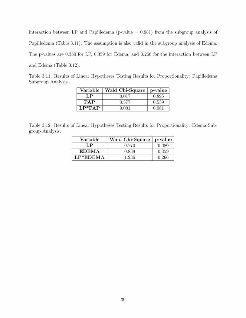
interaction between LP and Papilledema (p-value = 0.981) from the subgroup analysis of

Papilledema (Table 3.11). The assumption is also valid in the subgroup analysis of Edema.

The p-values are 0.380 for LP, 0.359 for Edema, and 0.266 for the interaction between LP

and Edema (Table 3.12).

Table 3.11: Results of Linear Hypotheses Testing Results for Proportionality: PapilledemaSubgroup Analysis.

Variable Wald Chi-Square p-valueLP 0.017 0.895

PAP 0.377 0.539LP*PAP 0.001 0.981

Table 3.12: Results of Linear Hypotheses Testing Results for Proportionality: Edema Sub-group Analysis.

Variable Wald Chi-Square p-valueLP 0.770 0.380

EDEMA 0.839 0.359LP*EDEMA 1.236 0.266

39

Chapter 4

Conclusion and Discussion

In this study, we conducted a retrospective analysis to assess the impact of lumbar puncture

(LP) on survival of comatose Malawian children. Overall, our analysis results showed no

impact on survival of the patients associated with LP. We found that after balancing the

treated (LP=1) and untreated (LP=0) groups using Papilledemia information, it did not re-

sult in a significant difference in the hospital death rates. Although exclusion of Papilledema

information from the statistical analysis resulted in the opposite conclusion (i.e. there is a

significant difference in the death rates), we considered Papilledema as an important covari-

ate in the analysis because the information is the primary element in making the decision

for performing LP. We also confirmed that different status in Papilledema and Edema does

not have a significant difference in the hazard of death between both treated and untreated

patients.

The LP data have a fundamental limitation, i.e. lack of randomness in the treated and

control groups, by the nature of observational study. We compensated this limitation by uti-

lizing propensity score (PS) methods. The propensity scores were estimated by using a linear

combination of 12 characteristic covariates. Through the PS method, we could obtained bal-

ance in covariates between treatment and control groups. We utilized the propensity score,

an average treatment effect for each subject, in two ways, i) inverse probability of treatment

weighting (IPTW) and ii) stratification. We found the same results, i.e. no significant evi-

dence of LP impact on survival of comatose patients with Papilledema information, through

40

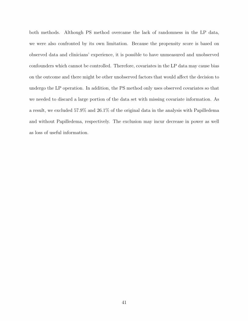
both methods. Although PS method overcame the lack of randomness in the LP data,

we were also confronted by its own limitation. Because the propensity score is based on

observed data and clinicians’ experience, it is possible to have unmeasured and unobserved

confounders which cannot be controlled. Therefore, covariates in the LP data may cause bias

on the outcome and there might be other unobserved factors that would affect the decision to

undergo the LP operation. In addition, the PS method only uses observed covariates so that

we needed to discard a large portion of the data set with missing covariate information. As

a result, we excluded 57.9% and 26.1% of the original data in the analysis with Papilledema

and without Papilledema, respectively. The exclusion may incur decrease in power as well

as loss of useful information.

41

BIBLIOGRAPHY

42

BIBLIOGRAPHY

[1] Joffe A.R. Lumbar puncture and brain herniation in acute bacterial meningitis: areview. Journal of Intensive Care Medicine, 22:194–207, 2007.

[2] Moxon C.A., Zhao L., Chenxi L., et al. Safety of lumbar puncture in comatose childrenwith clinical features of cerebral malaria. Neurology, 2016.

[3] D. Collett. Modelling Survival Data in Medical Research, Second Edition. Chapman &Hall/CRC Texts in Statistical Science. Taylor & Francis, 2003.

[4] Newton C.R., Kirkham F.J., Winstanley P.A., et al. Intracranial pressure in africanchildren with cerebral malaria. The Lancet, 337:573–576, 1991.

[5] Harrington D. Linear Rank Tests in Survival Analysis. John Wiley & Sons, Ltd, 2005.

[6] Cox D.R. Regression models and life tables. Journal of the Royal Statistical Society,34:187–220, 1972.

[7] Akpede G.O., Abiodun P.O., and Ambe J.P. Etiological considerations in the febrileunconscious child in the rainforest and arid regions of nigeria. East African MedicalJournal, 73:245–250, 1996.

[8] World Health Organization Multicentre Growth Reference Study Group. WHO ChildGrowth Standards: Methods and development. Geneva: World Health Organization,2006.

[9] Johns Hopkins Medicine. Lumbar puncture. Accessed: 2016-02-06.

[10] World Health Organization. Severe falciparum malaria. world health organization, com-municable diseases cluster. Society of Tropical Medicine and Hygiene, 94:S1–90, 2000.

[11] Austin P.C. An introduction to propensity score methods for reducing the effects ofconfounding in observational studies. multivariate behavioral research. MultivariateBehavioral Research, 46:399–424, 2011.

43

[12] Austin P.C. The use of propensity score methods with survival or time-to-event out-comes: reporting measures of effect similar to those used in randomized experiments.Statistics in Medicine, 33:1242–1258, 2014.

[13] Austin P.C., Grootendorst P., and Anderson G.M. A comparison of the ability ofdifferent propensity score models to balance measured variables between treated anduntreated subjects: a monte carlo study. Statistics in Medicine, 26:734–753, 2007.

[14] Rosenbaum P. R. and Rubin D. B. The central role of the propensity score in observa-tional studies for causal effects. Biometrika, 70:41–55, 1983.

[15] Black R.E., Cousens S., Johnson H.L., et al. Global, regional, and national causes ofchild mortality in 2008: a systematic analysis. Lancet, 375:1969–1987, 2010.

[16] P.R. Rosenbaum. Model-based direct adjustment. The Journal of the American Statis-tician, 82:387–394, 1987.

[17] P.R. Rosenbaum and D.B. Rubin. Reducing bias in observational studies using sub-classification on the propensity score. Journal of the American Statistical Association,79:516–524, 1984.

[18] Taylor T.E., Fu W.J., Carr R.A., et al. Differentiating the pathologies of cerebralmalaria by postmortem parasite counts. Nature Medicine, 10:143–145, 2004.

[19] van Crevel H., Hijdra A., and J. de Gans. Lumbar puncture and the risk of herniation:when should we first perform ct? Journal of Neurology, 249:129–137, 2002.

44