impact of tailings subsidence on rehabilitated landform ... · university of southern queensland...
TRANSCRIPT

University of Southern Queensland Faculty of Engineering and Surveying
Impact of tailings subsidence on rehabilitated landform erosional stability
A dissertation submitted by
Richard Houghton
In fulfilment of the requirements of
Course ENG4111 and 4112 Research Project
towards the degree of
Bachelor of Engineering (Civil)
Submitted: January, 2009

ii
Abstract
As a mine gets closer to the end of its productive life, rehabilitation of the site for its release back into the surrounding environment involves disposal of toxic, saturated fine grained tailings derive from ore processing. Tailings disposal back into the excavated pit and capping the site with a landform to isolate them from the environment is an accepted method of mine rehabilitation. The predicted long term stability of the landform due to the influence of tailings compression is a key factor to be considered in the design of the landform. The project investigates the settlement that had occurred at a mine site that was rehabilitated using this method of rehabilitation. The total settlement of the landform is quantified by comparing historical surface information to the existing surface level as determined by conducting a topographic survey. Current griding and mapping technology were also used to assist in the quantifying process. Using historic mine, landform design and construction information a consolidation model is presented base on Terzaghis one dimesional consolidation theory. This model is then calibrated to the landforms maximum recorded settlement. The findings presented provide a basis for further development towards designing capped tailings landforms with long term stability

iii

iv
Certification
I certify that the ideas, designs and experimental work, results, analyses and conclusions set out in this dissertation are entirely of my own effort, except where otherwise indicated and acknowledged.
I further crtify that the work is original and has not previously been submitted for assessment in any other course or institution, except where specifically stated
Richard John Houghton Student Number: 0019821368
_______________________________________________
Signature
_______________________________________________
Date

v
Contents
CERTIFICATION IV
LIST OF FIGURES VII
LIST OF TABLES IX
REFERENCES X
CHAPTER 1 – INTRODUCTION 1
1.1 Project Description 1
1.2 Aims 2
1.3 Specific Objectives 2
1.4 Background 2 1.4.1 Rum Jungle Mine 2 1.4.2 Ranger Uranium Mine 3
1.5 Literature Review 4
1.6 Methodology 5
CHAPTER 2 - UNDERSTANDING THE SETTLEMENT PROBLEM 6
2.1 Introduction 6
2.2 Geology and Historical pre-rehabilitation account of Dysons Open Cut 6
2.3 Design and construction Details of Dyson’s Rehabilitation Landform 9 2.3.1 Landform design details 9 2.3.2 Documented events during the landform construction 11
2.4 Geotechnical characteristics of the tailings materials 13 2.4.1 Pre rehabilitation impounded tailings at Dysons Open Cut 14 2.4.2 The Old Tailings Dam material 17 2.4.3 Conclusion 18

vi
CHAPTER 3 - DYSON’S OPEN CUT REHABILITATED LANDFORM SURVEYS 19
3.1 Introduction 19
3.2 Dyson’s Open Cut rehabilitated landform 2008 surface survey 19 3.2.1 2008 Survey Data Treatment 20
3.3 Dyson’s Open Cut rehabilitated landform 1986 as constructed survey 27 3.3.1 1986 Survey Data Treatment 27
3.4 Vertical alignment of the Georectified 2008 and 1986 raster data sets 28
3.5 Surface Mapping of the 2008 and 1986 Surveys 31 3.5.1 2008 Current surface 31 3.5.2 1986 surface 32
3.6 Determination of settlement magnitude 33
4.1 Introduction 40
4.2 Thezaghis Theory of one dimensional consolidation 40
4.3 Numerical solution to the one dimensional consolidation equation 45 4.4 Settlement model material properties discussion 51
Hard clay 52
4.5 Estimated material layer depths within the Cut and final landform overburden stress 57 4.5.1 Estimate of total stress to tailngs material at the location of maximum settlement 58 4.5.2 Estimate of the tailings thickness 60
4.6 Consolidation settlement model, results and discussion 60
4.6 Discussion of the model deficiencies 62
CHAPTER 5 - CONCLUSION 64
CHAPTER 6 - FURTHER WORK REQUIRED 65
APPENDICES 66
Appendix A - Project Specification 67
Appendix B - Site Photos and maps 70
Appendix C - Tailings material geotechnical data 76 Dysons Open Cut Geotechnical data taken from McNamara, (1984) 76
Appendix D – Model data results & 2008 Survey Data 88

vii
List of Figures
Figure 2.1 Dyson’s Open Cut Geology Map taken from Report of the working group
(1978)
Figure 2.2 Dysons landform design taken from McNamara (1984)
Figure 2.3 First tailings deposites to Dysons Open Cut 1984, taken from Allen & Verhoven (1986)
Figure 2.4 Dyson's existing in-pit Tailings, soil sample locations (McNamara 1984)
Figure 3.1 Dyson's Open Cut Rehabilitated Landform, June 2008
Figure 3.2 Existing survey monument
Figure 3.3 Landform at time of topographic survey
Figure 3.4 Dyson’s rehabilitated landform, between late 1984 & 1986
Figure 3.5 Tagged survey monument RL, Easing & Northing
Figure 3.6 Bore identification located adjacent to main batter slope
Figure 3.7 Survey setup location 2008
Figure 3.8 Dyson’s 2008 Survey Data Plot (X, Y) produced in Microsoft Excel
Figure 3.9 Geographical rectification of 2008 survey data to Dyson’s base map
coordinates system. 2008 Survey data points (Brown), published
coordinate location of bores (Yellow)
Figure 3.10 Digitised Contour map of Dyson’s rehabilitated landform 1986 (taken
from Allen & Verhoeven 1986)
Figure 3.11 Screen display of the process of geo-rectifying the digitised contour image and the geographical base map (extract from ArcMap software program)
Figure 3.12 Boundary defined Dyson’s landform 3-D surface from 2008 survey data created using the mapping software Golden Software Surfer.
Figure 3.13 Dyson’s 2008 Survey Data Contour map. Produced using Golden
Software Surfer mapping software. (1m Contour interval)
Figure 3.14 Boundary defined Dyson’s landform 3-D surface from 1986 survey data
created using the mapping software Golden Software Surfer
Figure 3.15 Dyson’s 1986 Survey Data Contour map. Produced using Golden
Software Surfer mapping software. Geographic coordinates have been
rectified (1m Contour interval)

viii
Figure 3.16 Dyson's surface overlay of 1986 & 2008 data showing difference in
height
Figure 3.17 1986 & 2008 contour map overlay with line showing cross section
(Produced in Golden Sofware Surfer)
Figure 3.18 Surface cross sectional plot, 1986 & 2008 surface data (Produced in
Golden Software Grapher)
Figure 3.19 1986 & 2008 contour map overlay with line showing cross section
(Produced in Golden Sofware Surfer)
Figure 3.20 Dyson's surface cross sectional plot, 1986 & 2008 surface data (Produced
in Golden Software Grapher)
Figure 4.1 Sketch of the consolidation process
Figure 4.2 Scematic of the finite difference method of estimation
Figure 4.3 Plot diagram of excess pore water pressure against vertical soil depth
(Parabolic curve)
Figure 4.4 Trapezoidal method of estimation of the integral of F(t)
Figure 4.5 Impermiable boundary condition allowance
Figure 4.6 Plot of one dimensional consolidation settlement against time

ix
List of Tables
Table 2.1 PSD data of existing tailings, Dyson's Open Cut (taken from McNamara, 1984)
Table 2.2 Static cone penetrometer derived shear strength
Table 4.1 Typical soil type coefficient of compressibility values (Smith C N,
2000). pg. 333
Table 4.2 Dyson's tailings estimated permeability from Hazen approximation equation
Table 2.3 Typical values of soil type permeability (Smith G N, 1990) pg 47
Table 4.4 Part Summary of geotechnical properties of tailings in Culmitzsch A (Wells, 2000)
Table 4.5 Estimated k-e relationship of clayey tailings (Wells C, 2000)
Table 4.6 Average Cv & Cc values for Cluff Lake tailings test plots (Hinshaw, 2004)
Table 4.7 comparison of fine grained tailigs Cv values from Table & Table
Table 4.8 Determination of cover material load stress
Table 4.9 Determination of fil material load stress

x
References
Verhoeven, TJ 1988, Rum Jungle rehabilitation Project Power and Water Authority,
Northern Territory.
Pidsley, SM (ed.) 2002, Rum Jungle Rehabilitation Project Monitoring, Report 1993 –
1998, Northern Territory Government, Department of Infrastructure, Planning and
Environment.
50
Barnekew V, Paul M & Jakubick AT 2002, Wismut GmbH, Technical Services,
Chemnitz, Germany, ‘Advanced Laboratory compression test & piezocone
measurements of time dependant consolidation of fine tailings’, Proceedings of the 9th
International Conference, Tailings & Mine Waste, fort Collins Colorado.
Zaar, U Farrow, R 2005, Catologue of Groundwater monitoring Bores in the Top End to
2005, Deptartment. of Natural Resources, Environment and the Arts, Nothern Territory.
Lowery, J & Staben, G 2007, Development of a GIS database and Metadatbase for
groundwater modelling and analysis of the Rum Jungle mine site, The Environment
Research Institute of the Supervising Scientist, Department of the Environment, Water,
Heritage and the Arts, Australia.
Allen, CG Verhoeven, TJ (ed), 1986 The Rum Jungle rehabilitation project final project
report, Department of Mines and Energy, Northern Territory.
Michael, E & Henderson PE 1999, ‘Control and optimisation of Tailings
Consolidation’, SRK Consulting Lakewood, Colorado, USA 80235.

xi
McNamara C, February 1984, Design Report, Rum Jungle Rehabilitation Stage 3,
Tailings Dam, Copper Heap Leach Pile and Dyson’s Open Cut, Northern Territory of
Australia, Department of Transport and Works.
Department of the Northern Territory, April 1978, Rehabilitation at Rum Jungle, Report
of The Working Group.
Mitchell, J K, 1993. Fundamentals of Soil Behaviour 2nd edn, John Wiley & Sons Inc,
N.Y.
Barneskow, U, Haase, M & Paul, M 2002 ‘Numerical simulation of consolidation and
deformation of pulpy fine slimes due to re-contouring and covering of large uranium
mill tailing ponds at Wismut’, Proceedings of the 9th International Conference, Tailings
& Mine Waste, fort Collins Colorado.
Wels, C 2000, A case study on self-weight consolidation of uranium tailings, Robertson
GeoConsultants Inc, Vancouver Canada.
Hinshaw, L 2004 ‘Tailings and Mine Waste ‘, Proceedings of the Eleventh Tailings and
Mine Waste Conference, Taylor & Francis Vail,Colorado, USA
Dames & Moore 1985, Report, Quality Control Testing, Stage 3, Whites Heap 3A
cover, Tailings Dam cover, Dysons Open Cut cover, Northern Territory, Australia
Department of the Northern Territory 1981, Rum Jungle rehabilitation project report of
the Working Group, Implementation Report Volume 2, Australia, p. 68
Mining & Process Engineering Services 1982, Engineering Report, Rum Jungle
Rehabilitation Project, Northern Territory

xii
Fourie, A & Tibbett, M (eds) 2006, ‘Assessing Landscape Reconstruction at the Ranger
Mine Using Landform Evolution Modelling’ Mine Closures 2006, Lowery J.B.C. et al.

1
Chapter 1 – Introduction
1.1 Project Description
This research project forms part of a larger project being established at the
Environmental Research Institute of the Supervising Scientist (ERISS). The waste bi-
products produced as a concequence of mining and ore milling operations are required
to be disposed of with minimal risk of polutent release to the surrounding environment
(mine rehabilitation). Mine tailings derived from the processing of extracted ore and
unprocessed rock (low grade ore or overburden rock) constitute the bulk of wastes to be
managed at mine closure. The land effected by the mining operation needs to be
rehabilitated for its return back the environment in which these contaminanted materials
are forever isolated.
One method of contained disposal at Pit excavation sites is to dispose of the tailings
material within the excavation. Further, constructing a landform above the pit (and
contents) to provide a cap, effectively isolating the wastes from adversely affecting the
immediate and surrounding environment is employed.
These tailings material are generally saturated and highly compressive. The
consolidation of the tailings material due to the load pressures generated by the above
landform cause surface sudsidence. This subsidence may cause breaching of the the cap
and release of contaminants to the environment. The long term stability of the landform
and cap is of primary concern with regard to mine rehabilitation.
This project (part of the overall project) investigates the settlement that has occurred at a
rehabilitated former mine site (of similar characteristics to that described above) to
aquire the knowelge to better predict the settlement magnitudes that are likely to occur
at similar type sites to which rehabilitation is yet to be implemented.
At the completion of mining at the Ranger Uranium mine (for details refer to
Backgroun following) Pits 1 and 3 will be capped with waste rock and laterite and
surcharged to accommodate tailings consolidation. As the landform matures, slope
angles and elevations may change as a result of consolidation. Currently landform
evolution modelling simulates change in elevation and slope resulting from erosion and
deposition only. Information is available to estimate consolidation rate i.e. (i) results of
tailings consolidation studies at Ranger, and (ii) through measurement of consolidation

2
and settlement that has occurred at the rehabilitated Dyson’s pit at Rum Jungle. Once
consolidation rate is estimated the rates of elevation change will be incorporated in
landform evolution model simulations of the Ranger landform focusing on development
in the first 20 years after construction.These results will be compared to simulations
which do not incorporate tailings consolidation to assess if there is an increased erosion
risk from cap settlement.
1.2 Aims
To estimate the likely extent of post-rehabilitation waste rock dump settlement as a
result of tailings consolidation/subsidence for use in simulating the effects of settlement
on long term erosion using landform evolution modelling.
1.3 Specific Objectives
This project part seaks to compare the predicted consolidation settlement to the
measured actual long term subsidence of the rehabilitated, Dysons Open Cut at Rum
Jungle Mining Lease. If the predicted and actual subsidence rates do not agree, an
investigation into modifying the prediction model parameters and apply for an
agreement with actual measured subsidence will be performed.
1.4 Background
1.4.1 Rum Jungle Mine
The Rum Jungle Mine is a former Uranium, Copper, Manganese, Lead and Zinc mining
lease that was operational between 1952 & 1971. It is located 85 km South of Darwin in
the headwaters of the East Branch of the Finniss River (Appendix B ). The site was left
in a heavily contaminated state causing significant environmental damage downstream
in the catchment. A degree of rehabilitation of the site was completed over a period
between 1982 and 1986 (Allen & Verhoeven, 1986).
Of particular interest at the site, is the Dysons Open Cut to which rehabilitation was
completed in late 1984. The Cut was used as the receptor of untreated tailings prior to
rehabilitation. As part of the rehabilitation of Dysons Open Cut it was further filled

3
with the tailings and contaminated subsoil from the leases heavily polluted old tailings
dam. On top of the tailings waste, a low grade copper ore and its associated
contaminated subsurface soils, from a failed experimental leach pad trial were placed to
form the bulk of the above ground landform. The Dysons fill was then capped, above
which a series of drainage and plant growth mediums were laid. The landform was
shaped with a gentle slope, continuous longitudinal grade and a transverse concave
grade that converged to a central diversion channel consisting of a rock mat stabilised
by wire mesh (Pidsley, 2002). Appendix B contains various diagrams and images of
Dysons open cut. The containment of contaminated materials, collection, and shedding
of excess water with minimal surface erosion, pooling of water and infiltration were the
main functional criteria to be met in rehabilitating Dysons open cut pit. Settlement of
the surface was recorded to have occurred as early as 1986 (Allen & Verhoven, 1986).
Further investigations in 1988 (Kraatz & Applegate, 1992) reported considerable site
settlement including a large area along the channel approximately 20m in length
subsiding to the degree that pooling of water during the monsoonal season was
occurring. later monitoring and investigation reports on the site identified revegetation
of Dysons’ landform as an increasing problem due to insufficient depth of plant growth
medium and the raising of acid mine water by capillary action from the oxidisation of
the underlying copper ore and associated contaminated soils (Pidsley, 2002). Increased
slopes developed through surface subsidence, combined with this loss of vegetative
cover is likely to be contributing to the significant surface scour that was noticed during
a visual site survey, post monsoonal season 2008 (Appendix B). Further exposure of the
copper ore material for oxidisation and transport of resulting acid material during future
heavy monsoonal rains may cause further increased pollution to the downstream Finniss
catchment.
1.4.2 Ranger Uranium Mine
The Ranger Uranium mine is an operational Uranium ore, open cut mining lease
surrounded by Kakadu National Park World Heritage area in the Northern Territory,
approximately 230 kilometres east of Darwin (Appendix B). The mine has been in
operation since the early 1980’s. The mine site consists of two open cut pits, ore body
No’s 1 and 3. Extraction from Pit No 1 has ceased and is now receiving the tailings from
the current open cut pit No 3 (the numbering of pits is associated with the ore deposit

4
No’s). When mineral extraction ceases from pit 3, the tailings housed in the tailings dam
will be deposited into pit 3. The broad rehabilitation proposal method involves capping
these contaminated tailing wastes essentially sealing them from the environment for up
to 10,000 years by preventing leaching, infiltration and subsequent water table rising.
Waste rock is then used to shape the bulked landform which is then overlayed with a
sequence of drainage, stabilising and vegetation supporting material zones. The final
shaped landform is to maintain plant growth and minimise the erosion impacts on the
downstream catchement ecosystem. Subsidence of the shaped landform may increase
the likelihood of adverse erosion and deposition affects on the surrounding, sensitive
ecosystem by way of a combination of surface erosion, vegetation dieback and down
catchement deposition.
1.5 Literature Review
There are two main processes by which soil settlement occurs, primary compression and
secondary compression (Mitchell, 1993 & Smith, 1990), Primary compression is
generally the first process by which soil volume decrease results. It is due to the excess
pore water pressure build up from stress loads applied at the surface of the soil.
Consolidation continues to occure until the excess pore pressure is balance with the
applied surface pressure. Consolidation duration is a function of how fast this excess
pressure can dissipate which is primarily a function of the soils permeability. Therefore,
saturated, low permeable soils (such as tailings) may undergo extended durations of
consolidation and therefore settlement (Mitchell, 1993 & Wels 2000). Secondary
compression involves involves the volume change of the soils due to changes in the
skeletal structure or creep (Mitchell, 1993).
Prediction of soil settlement due to consolidation was pioneered by Terzaghi with his
simple theory of soft soil consolidation (Mitchell, 1993 & Smith, 1990). The
assumption that make up the theory are that the soil is saturated, the void ratio and
effective stress relationship is linear and soil properties are assumed to not change
throughout the consolidation process (Mitchell, 1993). Lekha (2007) proposed a theory
based on Terzarghis but incorporating variable permeability and compressibility with
results that compaired well with laboratory testing.
The project involved aquiring historical information pertaining to the character,
quantified measures and historical accounts of events for the site of Dysons Open Cut.
5
The bulk of this information was obtained from two key documents (McNamara, 1984
and Alan & Verhoven 1986). Other documents reviewed are referenced throughout the
report.
1.6 Methodology
By sourcing and reviewing the historical reports and documents relating to the
rehabilitation of Rum Jungle Mine, a better understanding of the factors that have
influenced and contributed to the current settlement of Dysons landform was gained.
Measured quantities were extracted from this information for developing parameters
required for modelling the predicted settlement of the landform from construction
completion, to present day. Due to the lack of geotechnical data some key model
parameters were derived from those documented for mine sites of similar type and
character. A comprehensive topgraphic survey was undertaken of the current surface at
the Dysons rehabilitated landform. This information was compaired to the as
constructed surface information provided within a contour map of the landform. Current
gridding and mapping software technology was used to produce surface models to
quantify the total settlement over the full surface area. The settlement prediction model
was then calibrated by value manipulation of the coefficient of volume decrease until
the predicted settlement value equalled that of the observed maximum settlement.

6
Chapter 2 - Understanding the settlement problem
2.1 Introduction
This section was aimed at gaining a better understanding of the factors influencing the
settlement of the Dysons rehabilitation landform to assist modelling the landform
settlement due to the compression of underlying tailings. In the foregoing sections the
geology of the site, historical characteristic accounts, the design of the landform, events
encountered during the landforms construction, and geotechnical characteristics of the
tailings material below the landform were investigated for consideration with regard to
modeling the current landform settlement.
2.2 Geology and Historical pre-rehabilitation account of Dysons
Open Cut
Dyson’s open cut was used as a tailings repository on cessation of ore extraction in
1958. These un-neutralised, processed, uranium ore, tailings of unknown specific
characteristics were discharged into the Open Cut between the years of 1961 and 1965
(Allen & Verhoeven, 1986). The tailings were deposited into the pit via slurry pumping
and on ceasation of pumping the Cut was at its maximum holding capacity (Report of
The Working Group, 1978). The discharge point was located at the South Western end
of the cut and resulted in a beached sand zone forming around the discharge point. The
saturated finer material and waste water occupyied the remainder of the area (Report of
The Working Group, 1978). Therfore, it was assumed that these saturated finer
materials, sludge and slimes settled and accumulated further north into the deeper
sections of the cut coinciding with the location of the extracted, main ore body (Refer
Figure 2.5). In more recent years (closer to the time of rehabilitation) the tailings level
within the Cut was several meters below the cuts confines (Mining & Process
Engineering Servoces, 1982). Therefore, these impounded tailings material had
undergone an unquantified settlement due to consolidation under self weight loading.
Imediately prior to rehabilitation work the open cut was estimated to contain
approximately 20m in depth of saturated tailings (Department of mines and energy,
1984). Further Dysons Open Cut statistics of interst were as follows:

7
• Maximum cut depth: 45.7 m
• original volume: 0.92 x 10⁶ m3
• Weight of rock extracted (including ore and overburden): 2.5 x 10⁹ kg
• Unfilled volume: 0.7 x 10⁶ m3
Note: Volume estimates are accurate to +/-. 20 %
(Rum Jungle Rehabilitation Project, 1981)
Refering to the geology map of the Dysons site in Figure 2.5 a system of faults are
identified. For the this project, the fault system was assumed not to be a contributing
factor to the current landform settlement at the Dysons site and was ignored.

8
Figure 2.5 Dyson’s Open Cut Geology Map taken from Report of the working group (1978)

9
2.3 Design and construction Details of Dyson’s Rehabilitation
Landform
2.3.1 Landform design details
The design of Dysons landform and the associated design criterion were crucial factors
to be considered and understood in assessing the processes responsible for the current
settlement of the rehabilitation landform at Dysons Open Cut. The design cross
sectional drawings are presented in Figure 2.2 for reference.
Due to the toxic nature of the mine tailings derived from the processing of uranium ore,
isolation of this material from the environment was a primary design objective.
Therefore, with reference to Figure 2.2 the tailings fill were to be completely confined
within the Cuts boundary to a maximum level of 1m below the lowest point of its lip.
Disposal of the low grade copper ore and contaminated sub-soils from the nearby
Copper Heap Leach Pile were to be placed above the impounded tailings to form the
bulk of the landform. Due to the Pyritic nature of the low grade ore it required isolation.
Therefore preventing water circulating through it and providing a medium for acid
production by oxidation.
The percolation of rain and runoff water from the surface of the landform and capillary
rise of the excess pore water from the consolidation of the underlying tailings werer the
two main avenues for water ingress dealt with in the design. Reducing water ingress
from the top was dealt with by the slopping of the surface to prevent pooling, and
providing a low permeable, compacted clayey layer (zone 1A, Error! Reference
source not found.) directly above. The one meter, thick rock blanket, between the the
bulk landform and underlying tailings material was to act as an intercepting drain for
excess pore water expelled from the consolidation of tailings material below. Further a
series of intercepting drains and filter material layers were to contol the movement of
water through and around the landform (Cut off drain and 500 mm rock blanket, ). The
landform surface was sloped with a gentle cross fall towards the central rock lined drain
to collect and discharge surface runoff with minimal surface erosion (McNamara,
1984).
The tailings material was to be loosely place with some consolidation provided by the
earth moving equipement. The material constituting the bulk of the landform was to be

10
compacted to a modified dry density (MDD) of 95 %. However due to the expected low
bearing capacity of the loosly placed tailings the first two meters of the bulk fill was to
be compacted to the reduced MDD of 90 %.
From the above the following assumptions were made with regards to modelling the
settlement of the Dysons landform:
• The majority of currently observed settlement is due to consolidation of the
tailings material
• Settlement of the bulk fill material has contributed little to the current observed
settlement
• The base and sides of the Cut should be considered an impermiable boundary
• The surface of the tailings is the impermiable boundary for the settlement due to
consolidation
• External sources of pore water pressure do not exist

11
Figure 6.2 Dysons landform design taken from McNamara (1984)
2.3.2 Documented events during the landform construction
In order to better understand the processes by which the Dysons landform had settled
between the present day and construction completion, consideration of recorded
observations and events prior to and during the construction phase of Dysons
rehabilitation were considered to be of importance. Therefore, the following discussion
presents important historical accounts that were considered important to understanding
the settlement of Dysons landform for modelling purposes.
Prior to commencement of the sites rehabilitation program the North Eastern boundary
(the natural low point of the Open Cut) had been dammed to confine the un-neutralised,
saturated tailings and significant volumes of contaminated waste water. This retaining

12
structure was breached during the 1983/1984 wet season allowing the detained water to
drain (notably un-treated) into the East Branch of the Finniss River and out to the
Finniss River main. Prior to the construction process, a rock embankment was
constructed at the previously dammed, downstream location(removed to allow
discharge impounded water) to retain the tailings displaced by the filling operation of
the tailings material from the Old Tailings Dam site. Further up into the cut another
embankment was constructed to assist in retaining the liquefied tailings at the Cuts
centre (Allen & Verhoeven, 1986).
The filling operation utilised low displacement earthmoving equipment due to the
saturated, existing tailings high mobility potential. The imported tailings excavated
from the Old Tailings Dam site were placed into Dyson’s Open Cut commencing from
the Southern end, where the more stable, beached sand deposits (tailings discharge site)
were located (refer Figure 2.7 & Figure 2.8). Filling progressively advanced in the
direction of the Cuts low point (North East). The imported tailings were dumped onto
the previously placed tailings and the fill pushed forward in an attempt to assist the
expulsion of water vertically from the saturated, fine tailings. Therefore keeping the
highly saturated tailings material at the surface rising with the progressive fill level
(Allen & Verhoeven, 1986).
During the tailings placement operation there were many occurrences of surface
failures. These failures occurred as pools of liquefied tailings created due to the excess
pore pressures and the low shear strength of the material being placed, and that of the
underlaying tailings material. Strength failures on occasions saw the entire tailings fill
area liquefy to the point of flowing. On these occasions the rate of fill placement was
increased to displace this liquefied material towards the centre of the cut. To commence
placement of the Rock blanket material and subsequent fill it was necessary to place a
double course of geotextile fabric over this area to allow machinery access. The low
ground pressure Plant and equipment were replaced by conventional machinery once
sufficient material had been placed to produce a stable platform (Allen & Verhoeven,
1986).
With reference to the above accounts the central, deepest section of the Cut housed the
most unstable, saturated tailings material placed into the confines of Dysons Open Cut.
Further, the 2008 topographic survey showed that the region of the greatest settlement
coincided with this location.
13
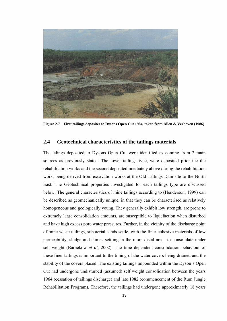
Figure 2.7 First tailings deposites to Dysons Open Cut 1984, taken from Allen & Verhoven (1986)
2.4 Geotechnical characteristics of the tailings materials
The talings deposited to Dysons Open Cut were identified as coming from 2 main
sources as previously stated. The lower tailings type, were deposited prior the the
rehabilitation works and the second deposited imediately above during the rehabilitation
work, being derived from excavation works at the Old Tailings Dam site to the North
East. The Geotechnical properties investigated for each tailings type are discussed
below. The general characteristics of mine tailings according to (Henderson, 1999) can
be described as geomechanically unique, in that they can be characterised as relatively
homogeneous and geologically young. They generally exhibit low strength, are prone to
extremely large consolidation amounts, are susceptible to liquefaction when disturbed
and have high excess pore water pressures. Further, in the vicinity of the discharge point
of mine waste tailings, sub aerial sands settle, with the finer cohesive materials of low
permeability, sludge and slimes settling in the more distal areas to consolidate under
self weight (Barnekow et al, 2002). The time dependent consolidation behaviour of
these finer tailings is important to the timing of the water covers being drained and the
stability of the covers placed. The existing tailings impounded within the Dyson’s Open
Cut had undergone undisturbed (assumed) self weight consolidation between the years
1964 (cessation of tailings discharge) and late 1982 (commencement of the Rum Jungle
Rehabilitation Program). Therefore, the tailings had undergone approximately 18 years

14
of self weight consolidation prior to rehabilitation works and loading of the impounded
tailings.
2.4.1 Pre rehabilitation impounded tailings at Dysons Open Cut
Geotechnical investigations were undertaken on the impounded, existing tailings
material within the Dyson’s Open Cut by Dames and Moore. The data and results were
documented in the design report, McNamara (1984). The geotechnical testing was
limited to the following:
• One hand auger hole to refusal at 0.45 m used for;
o Soil profile and chemical analysis
o Particle size analysis
o Plasticity Index
• Four Dynamic Cone Penetrometer tests and one (1) static cone penetrometer test
• Two Seismic refraction spreads
The Geotechnical report sheets are included in Apendix C
Investigations into the existing tailings material in the open cut were spatially limited
with regards to in situ testing and the testing of collected samples. Sampling and testing
was confined to one broad location over the area of the tailings deposits (Refer Figure
2.8). With reference to Figure 2.8, the sampling location approximately coincides with
the site of the tailings discharge point. Therefore, suggesting that the sampled material
was not truly representative of all the impounded tailings material present within the
cut. According to Barnekow, (2002) the material sampled was most likely that of the
larger granular sands that were first to settle out of suspension. According to the
geotechnical report in McNamara, (1984) the yellow/brown, existing tailings material
were classified as Silty Sands. The particle size distribution (PSD) results taken from
McNamara, (1984) are reproduced in Table 2.3. The data shows that the greater part of
the sample consisted of particles between 1.18 mm and 0.150 mm (fine sand).

15
Figure 2.8 Dyson's existing in-pit Tailings, soil sample locations (McNamara 1984).
The reported moisture content of the sample tested was 12.4 %, and the Atterberg limits
reported to be as the following:
• LL or WL = 0.28 or 28 %
• PL or WL = 0.24 or 24 %
• Plastic Index PI or I P = 0.28 – 0.24 = 0.04
Therefore, the tailings material at the site of investigation were found to be unsaturated
to an in situ depth of 450 mm. with a moisture content well below the plastic limit.
The estimated shear strength of the tailings from the static cone penetrometer test were
reported to be between 10 kPa and 12 kPa (Refer Table 2.2)
Area of significant settlement
Area of all soil sampling & testing
Region of historic Tailings discharge point

16
Sieve Aperture
(mm)
Mass Retained
(g)
Percent Retained (g)
Cumulative Percent Retained (g)
Percent Passing (%)
4.750 100
2.360 0.1 0.03 0.03 100
1.180 5.1 1.7 1.73 98
0.600 45.1 15.0 16.73 83
0.425 39.4 13.1 29.83 70
0.300 47.1 15.6 45.43 55
0.150 55.7 18.5 63.93 36
0.075 22.9 7.6 71.53 28.5
Pan 1.0 0.3 28.7
Fines washed out
28
Table 2.3 PSD data of existing tailings, Dyson's Open Cut (taken from McNamara, 1984)
The results of an investigations into the characteristics of pit impounded Uranium
tailings in Wels (2000) yielded the following results from laboratory testing for various
geotechnical properties. The testing was performed on essentially undisturbed samples
extracted by core drilling. The tailings were classified into course (sandy) and finer
(clayey) types:
1. Sandy classified as silty sands with typically less than 20 % particle diameter <
0.06 mm
2. Clayey with 50 – 60 % of clay sized particles of diameter < 0.006 mm

17
Test No. Location Depth (mm) Readings (Pounds Force)
Readings conversion to Newtons (N)
Estimated shear strength
(kPa)
6 Dysons Open Cut No.1
0
110 24.729 12
150 100 22.481 10
300 105 23.605 11
450 110 24.729 12
Average 106.25 23.886 11.25
Table 2.2 Static cone penetrometer derived shear strength
NOTE: Approximate conversion from Pound-Force to Newton: 0.22418lbf = 1N
2.4.2 The Old Tailings Dam material
From 1953 to early 1961 Tailings from the Uranium ore treatment plant (at the Rum
Junglle Mine site) were discharged, un-neutralised, to the adjacent Tailings dam area.
Approximately 640,000*103 kg of tailings material from the treatment plant were
deposited to a gently sloped area of approximately 30 hectares (300,000 m2). The
general tailings type was of finely ground, acid-leached waste from the processing of
Uranium and Copper ore (Allen & Verhoeven, 1986). The tailings had been subjected to
many years of seasonal flooding resulting in large volumes of the finest fraction along
with the slimes, and sludges being washed into the adjacent Finniss river. These tailings
were excavated from the dam site as part its rehabilitation and disposed of in Dysons
Open Cut as stated previously.
McNamara (1984) reports the following geotechnical testing was undertaken on this
tailings material:
• One 100 mm diameter auger hole to 2.3 m
o Soil profile and chemical analysis
o PSD
o Plasticity index
• Five dynamic cone penetrometer tests

18
• Five static cone penetrometer test
• One shear vane test
The Geotechnical report sheets are included in Apendix C
Unlike the limited spatial spread of the impounded Dysons tailings, the spatial spread of
sampling and testing covered representative areas of the entire tailings dam site
(McNamara 1984). Therefore, unlike the Dysons tailings the geotechnical results were
taken as, describing all material types present. The geotechnical report characterised the
grey tailings material as Sandy Silt (of finer fraction to the tailings in Dysons Cut) and
other results as follows:
• Moisture content = 20.8 %
• LL or WL = 0.25 or 25 %
• PL or WL = 0.21 or 21 %
• Plastic Index PI or I P = 0.25 – 0.21 = 0.04
• Remoulded shear strength between 1 and 5 kPa
(Refer to Appendix B for full result sheets)
2.4.3 Conclusion
The geotechnical investigation conducted on the two tailings material types that made
up the base soil layer of the Dysons landform were considered to be inadequate for
determining parameters for settlement modelling. Testing methods to quantify the
volume change behaviour of the tailings were not conducted. However, resulting from
the knowledge gained in this chapter, a better understanding of the factors that were
likely to have influenced the current differential settlement of the landform is achieved.

19
Chapter 3 - Dyson’s Open Cut Rehabilitated Landform Surveys
3.1 Introduction
To quantify the current subsidence of the Dysons landform, the as constructed and
current surface levels needed comparing. While the current survey information was
collected in the XYZ, point data format, the survey information of the as constructed
surface level was in the form of a basic contour map providing elevation information
only (Refer Figure ). The information type and format difference complicated the
comparison process. The contour map information needed digitising, geographical
alignement to the Dysons landform surface (as did the 2008 survey data, for reasons
detailed in the following sections) and interpolated surfaces created for both survey
data. The following sections detail the steps taken to compare the elevation information
from both surveys and quantify the settlement over the entire surface to the best
possible accuracy.
3.2 Dyson’s Open Cut rehabilitated landform 2008 surface survey
In early 2008 a visual site inspection of the Dyson’s Open Cut rehabilitated landform
was conducted. Large areas of the surface were thickly vegetated with tall grasses
making it difficult to evaluate the condition of the ground surface (Refer Figure 3.1).
However the general slope changes suggested that a substantial surface depression had
developed near the middle of the landform. This area of suspected subsidence possibly
coincided with the location of the main extracted ore body and the Cuts’ deepest
section. A comprehensive topographic survey was conducted in mid 2008 on the
landform using the Total Station, Topcon GTS-229 to quantify the subsidence. Almost
1700 XYZ point data were collected during the survey (Refer appendix C)
A problem was encounted prior to the commencement of the survey. Due to the isolated
nature of the site the location of an easily accessable, referenced datum (bench mark)
could not be found. During the initial site inspection two survey monuments were
located within the vicinity of the landform. The monuments consisted of a driven star
picket surrounded by concrete with a stamped brass annulus embedded (Refer Figure
3.), however, no additional identifying marks or identification numbers were attached.

20
The GPS coordinates were recorded at these monuments to assist in their identification
via registered survey or historical records (however as discussed later, no recorded
information for these features were found).
At the time of the topographic survey, fire had removed much of the vegetation
previously covering the landform and surrounds, (Refer Figure 3.). The bare landscape
more clearly highlighted the suspected surface depression as well as revealing
additional survey monuments and groundwater bores, all located adjacent to the base of
the main batter slope (Refer Figure 3.). One of these survey monuments had been
tagged with what was suspected as geodetic grid references and elevation (Refer Figure
3.). Additionally, identification numbers were attached to the bore casings (Refer Figure
3.). A permanent mark was installed on the top Eastern edge of the landform surface
with a clear, unimpeded visual of the entire Dyson’s surface, bores and the existing
survey monuments below the landform. The Total Station instrument was set up over
this mark, the tagged survey monument used as the backsight and all potential,
reference datum features picked up (Refer Figure ). Due to the uncertainty of the
reference coordinates attached to the backsite monument, arbitrary datum and grid
values were chosen with the veiw of editing the data when the information attached to
the tagged monument could be confirmed accurate.
An irregular survey point spacing was adopted, the number and spacing of points were
dictated by visual surface changes (the number of points increasing and spacing’s
decreasing in areas of prominent change in slope/elevation).
The collected survey data were downloaded via the Civilcad version 5.7 software and
saved to an Neutral (.NEU) file format compatible with software programs used for data
analysis. The data was imported to a Microsoft Excel spreadsheet and the X-Y data
plotted in order to highlight any gross errors or areas of insufficient data points and was
found to be satisfactory for further data treatment and mapping (Refer Figure ).
3.2.1 2008 Survey Data Treatment As mentioned above, arbitrary grid coordinates and height datum were used for the
2008 survey. To quantify settlement that had occurred, the two surveys (1986 & 2008)
needed to be spacially aligned to each other and surface level information compared.
The first step was to confirm the accuracy of the infromation attached to the backsight
used, then align the survey information to the Dysons landform, referenced to a gridded

21
map (base map) that would then become the common reference for the comparison.
This process is detailed in the following.
Using the gridding and mapping program ArcMap, the coordinates tagged to the back
sight monument used for the 2008 survey (Easting: 718740, Northing: 8563353) were
ploted on a grid map referenced in the Map Grid of Australia 1994, zone 52
(MGA94z52) coordinate system. The plotteded position however, was visually assessed
to be inacurate. The coordinates were found to be referenced to the Australian Geodetic
Datum 1984 (AGD84) and required conversion to the MGA94z52 coordinate system.
Replotting found the position of the monument to be reasonable, but the accuracy still
requiring confirmation. The current coordinates and elevation of the 2 bores picked up
in the survey were sourced in the Catalogue of Groundwater Monitoring Bores in the
Top End to 2005 (Zaar & Farrow, 2005). The positional accuracy of this information
was assessed with reference to the report by Lowery & Staben (2007), in which a
number of bores at the Rum Jungle site had been checked and validated for coordinate
accuracy. The Two bores however, were not among the list of those checked in the
report. Of the bores that were checked for positional accuracy (49 in total) the range of
positional difference to the published locations in Zaar and Farrow (2005) range
between 1 and 258 meters.
The published coordinates (Zaar Farrow, 2005) of the two bores were converted from
the AGD84 coordinate system to the MGA94z52 system and located on the base map.
The survey data was brought into the map, geographically rectified and pinned to the
map using the backsight MGA94z52 coordinates (Refer Figure 3.11). The 2008 survey
data points were rotated, pivoting at the backsight point to align the data with the
landforms central drain, being the most identifiable feature common to both the base
map and the surveyed points (Refer Figure 3.11). The surveyed bore points did not
coincide with the plotted position of the bores as seen in Figure. By using the distance
measuring feature of ArcMap the diffence between the ploted bore locations were found
to be three and seven meters. According to Lowery & Staben, (2007), this is not a
significant difference. Therefore the grid coordinates assigned to the backsight were
deemed to be sufficiently accurate and the 2008 survey data correctly aligned to the
base map. The 2008 survey points were assigned the corresponding base map
coordinates as defined by their location on the map.

22
The 2008 elevation data were aligned to the tagged monument (backsight) Z-value of
73.46 m. The 2008 elevation data of the two bores was checked against the published
elevations of Zaar and Farrow (2005). The difference in elevation was within 100mm
and accepted as accurate enough for the purposes of evaluating the settlement
magnitude of the Dyson’s landform. Finally, the point data was interpolated using the
kriging technique of estimation producing a raster data set for use in 3-D surface
modelling.
Figure 3.1 Dyson's Open Cut Rehabilitated Landform, June 2008.
Location of suspected depression

23
Figure 3.2 Existing survey monument
Figure 3.3 Landform at time of topographic survey
Location of suspected depression

24
Figure 3.4 Dyson’s rehabilitated landform, between late 1984 & 1986
Figure 3.5 Tagged survey monument RL, Easing & Northing
Main batter slope
Area were bores andsurvey monumentswere located
Approximate location of survey instrument

25
Figure 3.6 Bore identification located adjacent to main batter slope
Figure 3.7 Survey setup location 2008

26
Figure 3.8 Dyson’s 2008 Survey Data Plot (X, Y) produced in Microsoft Excel.
Figure 3.9 Geographical rectification of 2008 survey data to Dyson’s base map coordinates
system. 2008 Survey data points (Brown), published coordinate location of bores (Yellow)
Rum Jungle, Dyson's Rehabilitated Landform Surface Survey 2008
4850
4900
4950
5000
5050
5100
5150
5200
5250
300 400 500 600 700 800Arbitrary Northing
Tagged survey monument Bore
Bore
Arbitrary
Easting
Tagged monument

27
3.3 Dyson’s Open Cut rehabilitated landform 1986 as constructed
survey
As previously stated, the actual survey data for the as-constructed landform could not be
sourced, however, a contour map of the surface, taken at the time of the rehabilitation
landform completion was located in Allen & Verhoeven (1986), (Refer Figure 3.10).
This map had no other information attached to it with regards to the input survey data
and the method employed to produce it. However, as there were no other survey
information, the contour map was assumed to correctly model the surface elevation of
the Dyson’s Open Cut rehabilitated landform. In Allen & Verhoeven (1986) also
discussed, was the installation and use of permanent survey marks to monitor the
magnitude of the fills settlement and that these marks were used in the survey data
collection and its subsequent use for the contour maps production was assumed. These
same survey marks were assumed to be those located during the 2008 survey. With
regard to the above assumptions, it is likely that the 2008 survey data and the survey
data used in the production of the contour map referenced the same survey monument
height datum. Therefore determination of the settlement magnitude could be made by
directly comparing the 2008 and 1986 elevation values. The process of geographically
aligning the 1986 data to the reference base map is detailed in the following section.
3.3.1 1986 Survey Data Treatment
The 1986 contour map was required to be converted to a Digital Elevation Model
(DEM) for comparison to the 2008 survey data DEM. The contour map was first
scanned to create a digital image (.tif format File) and imported to the mapping and
editing software program ArcMap. The contour image file was then converted to a
raster image data set of 1.0 m square pixel/grid size. The map was positioned over the
coordinate base map of Dysons thereby geographically rectified (aligned) it to the base
map cordinates. To refine the alignment three points (triangle formation), easily
identifiable on both the base and contour image were selected and marked to the contour
image (Refer Figure 3.10Figure ). In turn, each point identified on the contour image
was dragged to its corresponding point on the base map and pinned. By this process, the

28
base map grid coordinates at the points new location were assigned to that same point
on the contour image. All grid points on the contoured raster image were now rectified
to the base map in 2-D space. The contours on the geographically rectified map were
traced, creating a shape file were each contour line was assigned its documented
elevation value. A Raster data file was then created from this geographically rectified
contoured file using the Special Analyst tool in ArcMap. The process produced an
imterpolated surface data set using an iterative finite difference interpolation technique
that could then be used to generate a three dimensional surface model of the landform.
3.4 Vertical alignment of the Georectified 2008 and 1986 raster data
sets
Through the processes described above the 2008 and 1986 raster data had been aligned
to a common base map coordinate system and the grid points assigned corresponding
cordinates. However, errors in the vertical alignment between the two data sets were
likely due to each alignment processes occurred independent of each. Therefore the
raster data sets were exported to the image processing software ENVI for layer stacking.
The layer stacking process involves an iterative sampling and realignment of the
pixel/grid data from both files bringing them into vertical alignment. A new banded file
is built from the georeferenced, raster data sets for a more accurate evaluation of
settlement magnitude over the time period between the two surveys. Finally, these
newly aligned files were exported to ASCII grid files of XYZ data.
29
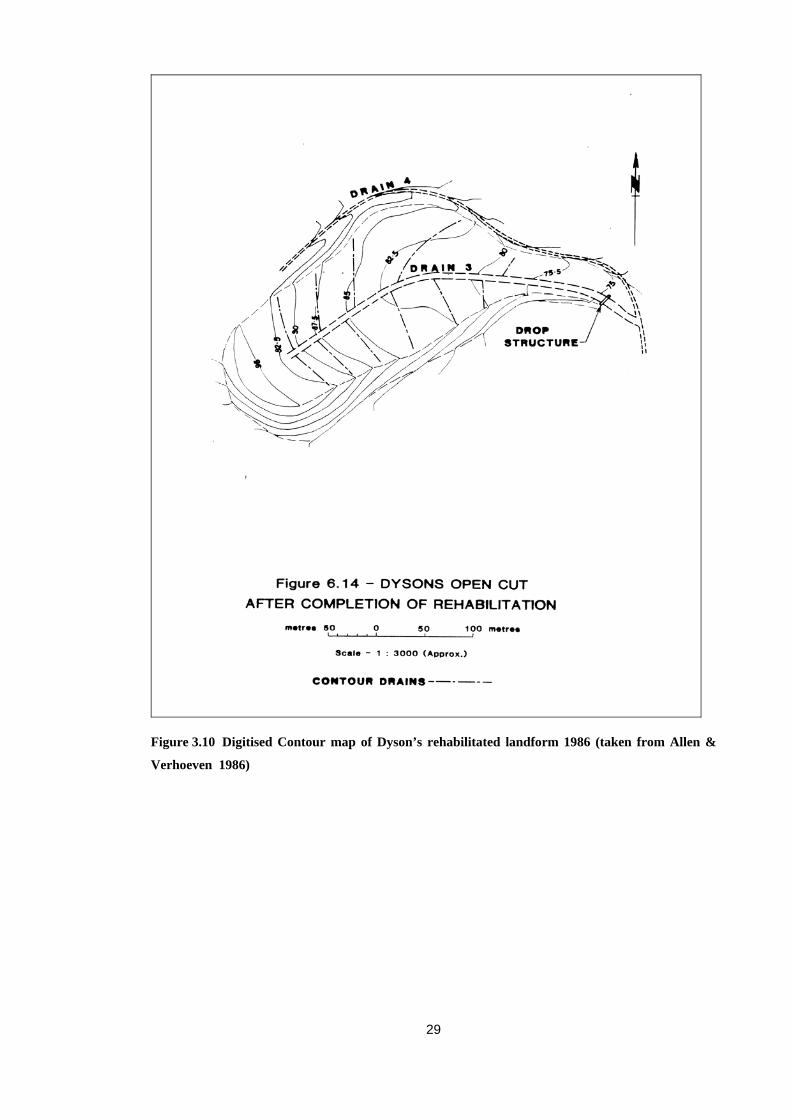
Figure 3.10 Digitised Contour map of Dyson’s rehabilitated landform 1986 (taken from Allen &
Verhoeven 1986)

30
Figure 3.11 Screen display of the process of geo-rectifying the digitised contour image and the
geographical base map (extract from ArcMap software program)

31
3.5 Surface Mapping of the 2008 and 1986 Surveys
Surface models created using the geographically rectified survey data from the above
processes and the process involved in their production is presented in the following.
3.5.1 2008 Current surface
The corrected Dyson’s 2008 survey data were imported to the grid and mapping
software, Golden Software Surfer to create a three dimensional surface and a contour
map of the landform in its current condition (Refer Figure & Figure ). A grid file was
created using the Nearest Neighbor gridding method, which assigns the values of the
nearest point to each grid node. Using this method allows the pixel data from the two
Raster surface files returned from the ENVI alignment process to be used directly as the
grid values. The three dimensional surface was then created using these grid file values.
The three dimensional surface model clearly shows the surface depression, the site of
excess settlement (Refer Figure ).
Figure 3.12 Boundary defined Dyson’s landform 3-D surface from 2008 survey data created using
the mapping software Golden Software Surfer.

32
Figure 3.13 Dyson’s 2008 Survey Data Contour map. Produced using Golden Software Surfer
mapping software. (1m Contour interval)
3.5.2 1986 surface
A three dimensional surface and contour model were also produced using the same
process employed for the 2008 models(Refer Figure & Figure ). The 1986 three
dimensional surface also shows a depression at the same location as the 2008 surface
Depression location

33
Figure 3.14 Boundary defined Dyson’s landform 3-D surface from 1986 survey data created using
the mapping software Golden Software Surfer.
Figure 3.15 Dyson’s 1986 Survey Data Contour map. Produced using Golden Software Surfer
mapping software. Geographic coordinates have been rectified (1m Contour interval)
3.6 Determination of settlement magnitude
Depression location

34
The two aligned surface data files (2008 & 1986) were used to create three dimensional
surfaces using ArcMap for the analysis and calculation of vertical settlement. The 1986
surface was identified as the reference plane and the difference between it and the 2008
surface were calculated. The analysis identified the areas of surface elevation change,
plotting the height difference between the two surfaces as colour delineated areas within
a value range (Figure 3.16). The area of maximum settlement (1.474m to 2.532m) is
identified as the approximate location of the extracted ore body and the deepest section
of the excavated Open Cut (the depression location as shown above in Figure to Figure
). It is to be noted that Figure shows significant settlement along the central collection
drain, however the central collection drain was not picked up in the 1986 survey and
hence was not included in the 1986 surface data used to produce the surface models.
The same central drain was included in both the 2008 survey and the surface models
produced from it, thus the difference values attached to the drain are not reliable.
Similarly, the surface water diversion banks show up in the model as areas of surface
bulging or soil deposition. For the purposes of settlement evaluation these features have
been ignored. Despite these two minor miss-representations the model clearly shows
significant settlement over most of the landform. An estimate of the maximum
settlement can be made by subtracting the depth of the channel from the range
maximum. From the reduced level point data, the depth of the channel is approximated
as 800 mm, thus a maximum settlement of 1800 mm can be estimated.

35
Figure 3.16 Dyson's surface overlay of 1986 & 2008 data showing difference in height
Sections were taken throught the landform (Figure & Figure ), using the mapping and
graphing software program Surfer. The location of these sections are shown in Figure
and Figure 3.19.
Section A-A was made approximately perpendicular, and through, the central collecting
channel (Refer Figure ). The cross sectional data from the two surfaces, plotted together
in Figure clearly shows the elevation difference between the 1986 surface level
compaired with the existing 2008 surface. As noted previously the elevation comparison
is missrepresented due to the central drain elevation data being included in the 2008
survey but omitted from the original 1986 survey. To evaluate the maximum settlement
from the plot in Figure , the central channel on the 2008 line plot needed to be ignored.
Scaling the maximum vertical difference on the plot in Figure , against the y-axis gives
an approximate 2000 mm settlement value.
Surface water diversion banks

36
Figure 3.17 1986 & 2008 contour map overlay with line showing cross section. (Produced in
Golden Sofware Surfer)
2008 Surface
1986 Surface
A
A

37
Figure 3.18 Surface cross sectional plot, 1986 & 2008 surface data (Produced in Golden Software
Grapher)
Section B-B was made in a direction approximately parallel to the central collection
drain but did not include it in the cross sectional data (Refer Figure 3.19). The cross
sectional plot generated and shown in Figure also indicates a settlement value of
approximately 2000 mm.
The above three methods of analysing the surface elevation difference to determining
the settlement magnitude of the Dyson’s rehabilitated landform over the 22 year period
between the years 1986 and 2008 yielded similar values and is taken to be 2000 mm.
A
A
2000 mm

38
Figure 3.19 1986 & 2008 contour map overlay with line showing cross section. (Produced in
Golden Sofware Surfer)
2008 Surface
1986 Surface
B
B

39
Figure 3.20 Dyson's surface cross sectional plot, 1986 & 2008 surface data (Produced in Golden
Software Grapher)
B
B 2000 mm
40
Chapter 4 - Model estimate of landform settlement due
to compression of underlain mine waste tailings
4.1 Introduction
In the previous sections differential surface settlement of Dyson’s landform has been
shown to have occurred. The quantified maximum settlement was also shown to
coincide with the Cuts deepest section and the likely location of the saturated finer
grained, sludge and slime tailings material placed into Dysons Open Cut. Further,
substantial gully erosion was identified in this maximum settlement zone with the
remainder of the surface showing only minor signs of erosional effects. Therefore the
area of observed maximum settlement is of primary interest. Given that little knowledge
of the tailings geotechnical properties exist calibrating a settlement model to the
observed settlement is difficult, if not impossible. However, since the construction
records documented the tailings condition as being saturated and highly unstable at the
time of the fill being placed above the tailings, settlement due to the process of
consolidation will be discussed. Further to this, only one dimensional consolidation is
considered as a preliminary to possible further work to aquire better geotechnical
knowledge of the tailings. In the following section the simple theory of one dimensional
consolidation by Tezaghi (1945) is presented together with a simple numerical solution
to this theory for modeling consolidation settlement. The required input factors for the
model (with respect to the tailings material) are discussed and estimated. The model is
then used to simulate the the landforms settlement at the maximum observed settlement
zone by manipulating the governing factor. Finally the results and deficiencies of the
model are discussed.
4.2 Thezaghis Theory of one dimensional consolidation
The simplified linear and elastic consolidation theory for fine grained soils by Tezaghi
(1945) is well documented and has been the basis for estimating the settlement
magnitude of soft soil layers due to consolidation and the rate at which it occurs.
Allthough the theory is heavily simplified using assumptions that somewhat detract
from the realistic processes that occur during consolidation settlement, the application

41
of the theory can, in some cases return reasonable estimates of actual settlement (Smith
1990) The simple theory is presented here for a preliminary evaluation of settlement
modelling.
The main assumptions in the theory are:
1. The soil is essentially homogenous and saturated
2. Both the soil pore water and soil particles are incompressible
3. The coefficient of consolidation is held constant
4. Darcy’s law of saturated flow is applied and valid
5. The compression induced consolidation is one dimensional (vertical down) only
6. Expulsion of water from the soil voids is in one direction only (Vertical)
7. Volume change of soil is only due to a change in the void ratio, which in turn is
due to a corresponding increase change in the effective stress. The relationship
between void ratio ( e ) and effective stress ( 'σ ) is linear
8. There is no instantaneous volume change on application of the overburden
pressure increase (Total stress increase)
To visualise the consolidation processes assumed, the problem of one dimensional
consolidation is shown in Figure 4.1.

42
Figure 4.1 Sketch of the consolidation process
The rate of volume decrease (settlement) of the soil is equal to the rate at which the
fluid in the soil pores flows out due to the constant stress applied by the tailings layer
overburden. Darcy’s law is valid therefore the pore fluid velocity (v) is evaluated from:
zhkv∂∂
=
Where: =k Soils Coefficient of Permeability, vertical (z) direction
=h Hydrostatic pressure head causing flow
=z Vertical soil thickness
The head causing flow ( )h is the excess pore water pressures in the soil medium thus:
w
uhγ
=
Where: =u Excess pore water pressure
=wγ Unit weight of water
Therefore the change rate of volume becomes:
2
2
zuk
zuk
z ww ∂∂
=∂∂
∂∂
γγ
Impermeable boundary (base)
Fine grained tailings
Top of tailings fill
Total stress load (q)
Permeable boundary
H

43
As the volume change is assumed to occur due to the change in void ratio (e) over time,
the change rate of volume may be expressed in terms of the void ratio as follows:
Soil Porosity e
eVVn v
+==
1
Change rate of volumete
e ∂∂
+=
11
Equating the two equations gives the equation of consolidation:
te
ezuk
w ∂∂
+=
∂∂
11
2
2
γ
The overburden pressure is equal to an increment of applied pressure (dp) and together
with the assumption that no lateral strains exist then dp is equal to, but opposite in sign
to the resultant increment of excess pore water pressure (du)
The slope of the void ratio – effective pressure (e – p) curve derived from a
consolidation test being the coefficient of consolidation (Cv)
dude
dpdeCv =−= then duCde v=
The coefficient of consolidation may also be represented as:
( )vww
v mkekC
γγ=+= 1
Where: mv = Coefficient of volume decrease. That is the unit volume decrease per
unit increase in effective pressure.
Therefore substituting:
tu
zuCv ∂
∂=
∂∂
2
2
OR tum
zuk
vw ∂
∂=
∂∂
2
2
γ
The above equation is a one dimensional and linear partial differential equation
The analytical solution to the above equation gives the value of excess pore water
pressure (u) at depth (z) and at time (t).

44
( ) Tα
0
2nsin12 −
∞
=∑= eZqu nn n
αα
Where: ( )πα 1221
+= nn
HzZ = (dimensionless distance factor)
2HtCT v= ( dimensionless time factor)
=H The maximum distance water is required to travel within the soil
depth.

45
The vertical surface settlement of the full depth soil layer can be given by summing all
the vertical strains of the infinitely small soil layers constituting the full soil depth and is
represented by:
( ) zduqmSH
v∫ −=0
Where: q = the applied load at the surface of the soil and,
mv is assumed constant.
Then substituting:
( ) dzeZqmSH
nn n
v ∫ ∑ ⎥⎦
⎤⎢⎣
⎡−= −
∞
=0
Tα
0
2nsin121 α
α
The integral gives:
⎥⎥⎦
⎤
⎢⎢⎣
⎡−=
−∞
=∑
nnv
eqHmSα
Tα
0
2n
21
The above equation gives the surface settlement due to consolidation at any time over
the full layer depth.
The required evaluation of the integral analytically may be substituted by numerical
techniques as described in the following section.
4.3 Numerical solution to the one dimensional consolidation
equation
A simple numerical solution to the one dimensional consolidation equation can be
achieved using the finite difference method of approximations. By the use of this
method the excess pore water pressures at specified points in time and space (soil depth)
are evaluated. (Refer Figure )

46
Figure 4.2 Scematic of the finite difference method of estimation
To illustrate the finite difference method and its application to the one dimensional
consolidation equation we can assume that the excess pore water pressure over the full
range of the soil depth approximates a parabolic shape when the variation of u with z is
plotted (Refer Figure ).
t=t0 t=t1 t=t2 t=t3 t=t4 dt
dz
z=z0
z=z2
z=z3
z=z4
z=z1
t
z
uz,t
uz+1,t
uz+2,t
uz+3,t
uz+4,t
uz+1,t+1
uz,t+1
uz+2,t+1
uz+3,t+1
uz+4,t+1
uz+1,t+2
uz+2,t+2
uz+3,t+2
uz+4,t+2
uz,t+2 uz,t+3 uz,t+4
uz+1,t+3 uz+1,t+4
uz+2,t+3 uz+2,t+4
uz+3,t+3 uz+3,t+4
uz+4,t+3 uz+4,t+4

47
Figure 4.3 Plot diagram of excess pore water pressure against vertical soil depth (Parabolic
curve)
Therefore the parabolic equation becomes:
u = a1 + a2z + a3z2
Where: a1, a2 and a3 are fitted constants
Evaluating the excess pore water pressures (u), from the reference position of Point B in
Figure :
u at point A = a1 – a2dz + a3dz2;
u at point B = a1
u at point C = a1 + a2dz + a3dz2
Then relating the constants (a) to the points of interest in Figure :
Bua =1
z = -dz
z = 0
z = +dz
Assumed parabolic shape of u with
depth z
Point A
Point B
Point C
Increasing z
uC
uB
uA
Increasing u

48
dzuua AC
22−
=
23 22
dzuuua BCA −+
=
Then the slope of u at point B is: dz
uuzu AC
B 2−
=⎥⎦⎤
⎢⎣⎡∂∂
The curvature at point B is: 22
2 2dz
uuuzu BCA
B
−+=⎥
⎦
⎤⎢⎣
⎡∂∂
Using the above equation for the curvature at point B and relating it to the one
dimensional, partial derivative, consolidation equation:
tu
zuCv ∂
∂=
∂∂
2
2
,
and the excess pore water pressure at point B can be expressed as:
22
2 2dz
uuuCzu BCA
vB
−+=⎥
⎦
⎤⎢⎣
⎡∂∂
Then by integrating the previous equation over the period of t to t +dt, the change in
pore water pressure at point B is evaluated by the following equation:
( )∫+
−++=dtt
tBcA
vBB dtuuu
dzCdqdu 22

49
The integral in the previous equation is approximated by assuming the integral of the
time function over the time step is approximately equal to the function of t, multiplied
by the time step (trapezoid method) which is graphically represented in Figure below.
Figure 4.4 Trapezoidal method of estimation of the integral of F(t)
In its simplified form the equation then can be expressed as:
( ) ( ) ( ) ( )[ ]tututudqdttu BCBBB 2−++=+ β
Where: 2ztCv
ΔΔ
=β
For the case where the lower boundary being considered impermeable the above
equation is further simplified to:
( ) ( ) ( )[ ]tutudqdttu CABB ++=+ β
F(t)
t t t +dt
Error in time step shaded
Area below the curve approximately = F(t) x dt

50
There is a stability issue with the use of the above equation. The condition if not
adhered to will become unstable with the results being invalid.
The stability condition to be followed is:
5.02 ≤ΔΔ
=z
tCvβ
The results for the excess pore pressure dissipation rate is dependent on the flow path
distance to a permeable boundary for expulsion of the pore water and subsequent
increase effective stress required for induce settlement.
For the boundary condition of:
• Lower boundary (Open Cut base) is assumed impermeable
• Upper boundary (Interface of tailings deposit and rock drainage
mattress) assumed permeable
At the assumed impermeable boundary 0=∂∂
zu , as there can be no water flow across
this boundary (Refer Figure ).
Figure 4.5 Impermiable boundary condition allowance
With reference to Figure , using the finite difference approach and letting 5.0=β :
dz
dz
point A
point B
point C
Impermeable base
Tailings top
z = H

51
At point B, dz
uuzu AC
20 −
==∂∂
Then: uA = uC must be the resulting case
Therefore it is necessary to place a fictitious point (point C in Figure 4.5), below the
impermeable base point for the progression of the finite difference approximation of the
excess pore water pressure through time and layer depth.
The equation for estimation of the settlement magnitude (S), with constant mv and q
then becomes:
( )∫ ∫−=−=H H
vvv dzumqHmdzuqmS0 0
Since the finite difference method evaluates the excess pore pressures at specified points
in time and space on an established grid system, the integral of u can not be evaluated
exactly however the trapezoidal approximation method as described previously can be
used as follows:
( ) ( )dzuudzuudzu nn
H++++≈ −∫ 1100
5.0...5.0
4.4 Settlement model material properties discussion
As described previously the geotechnical data collected prior to the rehabilitation works
for the processed tailings material placed into Dyson’s Open Cut was sparse. The
geotechnical investigation did not include any compression or consolidation testing for
the assessment of soil volume change behaviour. Further, the surface area spread of the
investigation on the in situ tailings material within the Cut was confined to the likely
location of the courser, more stable (less compressible) material. Therefore, the finer
grained, more compressible tailings material was neglected. What can realistically be
gained from the geotechnical data recorded for the tailings material is that its shear
strength is very low, suggesting an even lower shear etrength characteristic for the fine
grained, slurry tailings of interest. Coupled with this lack of soil property knowledge,
depths of the materials that existed and placed within the Cut at the time of construction

52
were not recorded and therefore unknown. Therefore, an estimation of the overburden
pressures placed on the tailings layer was required.
Soil properties that can be considered essential to utilising any settlement model are
generally derived from various compression and consolidation testing methods. Such
volume change behaviour parameters tested for are:
• Permeability (k)
• Void ratio (e)
• Compression index (Cc)
• Coefficient of consolidation (Cv)
• Coefficient of volume compressibility/decrease (mv)
None of the above soil volume change parameters were investigate for with regard to
the tailings material placed below the landform. Therefore, representative, typical or
assumed values are required for input to the model for settlement evaluation. A
discussion on the possible use of typical volume change parameters follows.
Typical values of mv for the general soil types, presented in Smith (1990) are
reproduced in Table 4.1.
Table 4.1 Typical soil type coefficient of compressibility values (Smith C N, 2000). pg. 333
With reference to Figure 4.1 above, the coefficient of volume compressibility for the
fine grained tailings material in Dyson's Open Cut are likely to fall into the large range
mv range (m2 / kN) Soil Type
from to
Peat 0.01 0.002
Plastic clay (normally consolidated alluvial
clays)
0.002 0.00025
Stiff clay 0.00025 0.000125
Hard clay
0.000125 0.0000625

53
of values attributed to the Plastic clay or Peat soil types. The values in the above table
are usefull for identifying gross errors of the coefficient only.
Since the permeability of a soil depends on the soils porosity, which in turn is related to
the soils particle size distribution (PSD), an estimate of the soils permeability can be
arrived at using the soils PSD data.
Hazen (1892) proposed the following emperical formula to estimate the permeability of
a soil based on its PSD data:
smmDk /10 210=
Where: =10D effective size in mm (largest size of the smallest 10%).
Using the above equation it is possible to determine an approximate value of
permeability for the reported sandy silt and silty sand tailings material using the PSD
data in McNamara C, (1984) (Refer Appendix C). However the particle size analysis
was restricted to the the smallest sieve aperture of 0.075 mm used. The sample
percentage passing (for both soils) the 0.075 mm sieve were greater than the 10%
required by the Hazen formula. However, to illustrate the inaccuracy of using this
formula the formula results are presented in Table 4.2.
Tailings source Soil Classification % retained on 0.075mm sieve
k (Hazen 1892)
Old tailings dam Sandy Silt 63.3 5.625*10-5
Dyson’s Open Cut Silty Sand 28.5 5.625*10-5
Table 4.2 Dyson's tailings estimated permeability from Hazen approximation equation
Comparing the values in Table 4.2 to typical values of permeability for general soil
types presented in Table 4 (Smith, 1990), The permeability value returned by the
equation at the boundary of the fine sand, course silt permeability range. Given, that the
percentage of the material passing the 0.075 mm sieve was also well in excess of the
10% required suggests the permeability for both soils is well below that calculated.
Therefore the emperical equation is of no real use in this case.

54
Soil Type Permeability Range (k)
(m/s)
Gravel >10-1
Sands 10-1 – 10-5
Fine Sands, Course silts 10-5 – 10-7
Silts 10-7 – 10-9
Clays < 10-9
Table 4.3 Typical values of soil type permeability (Smith G N, 1990) pg 47
From Table 4 above, the saturated fine grained tailings of interest would likely fall in to
the silts and clays soil types values. These values while usefull for identifying gross
error, are of little use for determining a representative permeability value for the
tailings.
Another possible method to attribute reasonable soil property values for the fine tailings
in Dyson’s open Cut is to evaluate the reported properties of Uranium tailings at other
mine sites to which rehabilitation and or rehabilitation studies have commenced. One
such mine site is the former Uranium mine in Eastern Thringia, Germany. The
Culmitzsch A tailings impoundment, itself a former open cut, received milled tailings
between the years 1967 and 1991. (Wels, 2000)
A portion of the averaged laboratory test results to determine the geotechnical properties
of the impounded tailings documented in Wels C, (2000) are presented in Table . The
laboratory tests were performed on undisturbed samples retrieved through an extensive
drilling program. The tailings material were classified into two main types, course
tailings and clay rich tailings as follows:
1. Clayey Typically 50-60% clay sized particles (diameter < 0.006mm)
2. Silty sands Typically < 20% silt sized particles (diameter < 0.06mm)

55
Water content
Void Ratio
Attergerg limits
Plasticity Index
Shear strength
Tailings Type
Description
w e wP wL IP (kN/m2)
Average 0.851 2.437 0.258 0.657 0.399 12
Max. 0.366 1.034 0.178 0.366 0.182 0
Clayey variety
Min. 1.621 4.788 0.293 0.846 0.553 42
Average 0.248 0.774 0.181 0.354 0.167 20
Max. 0.176 0.549 0.169 0.316 0.138 8
Sandy variety
Min. 0.405 1.186 0.195 0.391 0.195 35
Coefficient of Consolidation
(Cv) m2/s
Tailings
Types
Description Compressi-on index Cc
Stress =47kPa Stress = 174kPa
Hydraulic Conductivity (k) m/s
Range 0.6 - 0.8 2 - 7*10-7 1 - 9*10-7 2*10-9 - 6*10-6
Clayey variety
Void ratio 1.2 - 3.2 1.4 - 2.9 1.3 – 2.1 0.9 – 3.0
Range 0.02 - 0.08 3*10-7 -1*10-6 3*10-7 – 1*10-6 9*10-7 – 3*10-5
Sandy variety
Void ratio 0.7 - 0.9 0.5 - 0.9 0.5 – 0.9 0.6 – 1.2
Table 4.4 Part Summary of geotechnical properties of tailings in Culmitzsch A (Wells, 2000)
The values in Table show a large difference between the sandy and clayey tailings. The
range of property values for each variety are also large but may be of some use in
arriving at an estimate Cv of the tailings in Dyson’s for use in modelling consolidation
settlement.
The hydraulic conductivity values (k), in Table , for the clayey tailings variety were
derived from the standard permeameter test and were considered unreliable so further
tests were conducted using a specially designed slurry consolidometer (Wells, 2004).
The results of this testing are shown in Table .

56
Void Ratio (e) Permiability or
Hydraulic Conductivity
(k) (m/s)
4.0 4 – 7*10-7
3.0 3 – 5*10-8
2.0 2 – 4*10-9
1.5 3 – 6*10-10
Table 4.5 Estimated k-e relationship of clayey tailings (Wells C, 2000)
Comparing the two sets of values for k, the results in Table show a similar permeable
soil for the void ratio range than those reported in Table .
Another former Uranium mine of interest is the Cluff Lake Uranium mine in Canada
which ceased operation in 2002. Settlement studies have been conducted with regard to
the fine grained tailings placed within in a raised embankment facility lined with an
impervious clay base. Dykes separate the courser sandy type tailings and the finer
grained, sludge type tailings. Full scale test plots of approximately 50m by 50m were
constructed and settlement due to controlled cover placement was monitored via survey
control points and bore holes housing piezometer nests for pore water pressure
assessment within the plots. The data collected was used to determine estimates of the
coefficient of consolidation and compression index using the theory of one dimensional
consolidation. The values reported are presented in Table 4.6. (Hinshaw L, 2004)
Consolidation Parameter
Average Minimum Maximum
Coefficient of Consolidation (Cv) (m2/day)
0.024 0.020 0.028
Compression Index 2.07 1.48 2.73
Table 4.6 Average Cv & Cc values for Cluff Lake tailings test plots (Hinshaw, 2004)

57
A Comparison of the Cv results from the above two tables is presented in Table :
Fine Tailings Cv Values
Table
Void Ratio Range m2/s m2/day m2/year
4 1*10-7 0.009 3.154
4 2*10-7 0.017 6.307
4 3*10-7 0.026 9.461
4 4*10-7 0.035 12.614
4 5*10-7 0.043 15.768
4 6*10-7 0.052 18.922
4 7*10-7 0.060 22.075
4 8*10-7 0.069 25.229
4
1.3 - 2.1
9*10-7 0.078 28.382
Average 1.7 5*10-7 0.043 0.078
6 2.8*10-7 0.024 8.760
Table 4.7 comparison of fine grained tailigs Cv values from Table & Table
The above discussion of general soil Uranium derived tailings geotechnical properties,
essentially means that representative values of k, e, Cc, Cv or mv for Uranium ore
derived tailings can not be arrive at. This is mainly due to factors such as the varying
ore properties and the processing method that the tailings were derived from. Other
factors such as temperature, pore water chemistry, physiochemical interactions,
chemical precipitate induced particle cementation will contribute to variability
(Mitchel, 2000).
4.5 Estimated material layer depths within the Cut and final
landform overburden stress
Due to the sloping nature of Dysons landform the fill material placed over the full
tailings area, within the Cut’s confines varies in depth spacially. Therfore the value of
the total load stress applied at the surface of the tailings also varies spacially. Excluding

58
the cover materials of fill zones 1A, 1B, 2A and the rock blanket, historical records of
the fill material depths, in any section of the constructed landform were not obtainable.
Therefore, a reasonable estimate of placed fill depths (at the location of maximum
observed settlement) was required for the calculation of the total stress, as applied to the
surface of the tailings layer.
From the historical records obtained the tailings materials were placed to a maximum
height of one meter below the Cut’s rim, at its lowest point (Allen & Verhoeven, 1986).
The final maximum excavated depth was documented as 45.7m (Davey, 1975 &
Verhoeven, 1988). However no datum was linked to the above measures for quantifying
of the tailings thickness. Therefore, the maximum drainage path for the one dimensional
consolidation equation is not readily obtainable. Resulting from the above, a basic
estimate of the material thicknesses was required for input to the settlement model. The
method is described in the following:
4.5.1 Estimate of total stress to tailngs material at the location of maximum
settlement
Working from the surface of the landform down through the stratum the following
material thickness and associated stress loadings were estimated.
The contribution of the uppermost cover to the total load stress as applied to the tailings
layer were calculated using average soil density data from in situ testing conducted at
the time of construction (Dames & Moore, 1985). (Refer Table 4.8)
Material Description
Averged Placed Thickness (m)
Averaged in situ Density (kg/m3)
Resulting Averaged Load Stress (kPa)
Zone 2A 0.170 2250 3.752
Zone 1B 0.350 1980 6.798
Zone 1A 0.380 1840 6.823
Totals 0.900 17.373
Table 4.8 Determination of cover material load stress
The bulk of the fill material placed between the cover and tailings layers came from two
main sources:
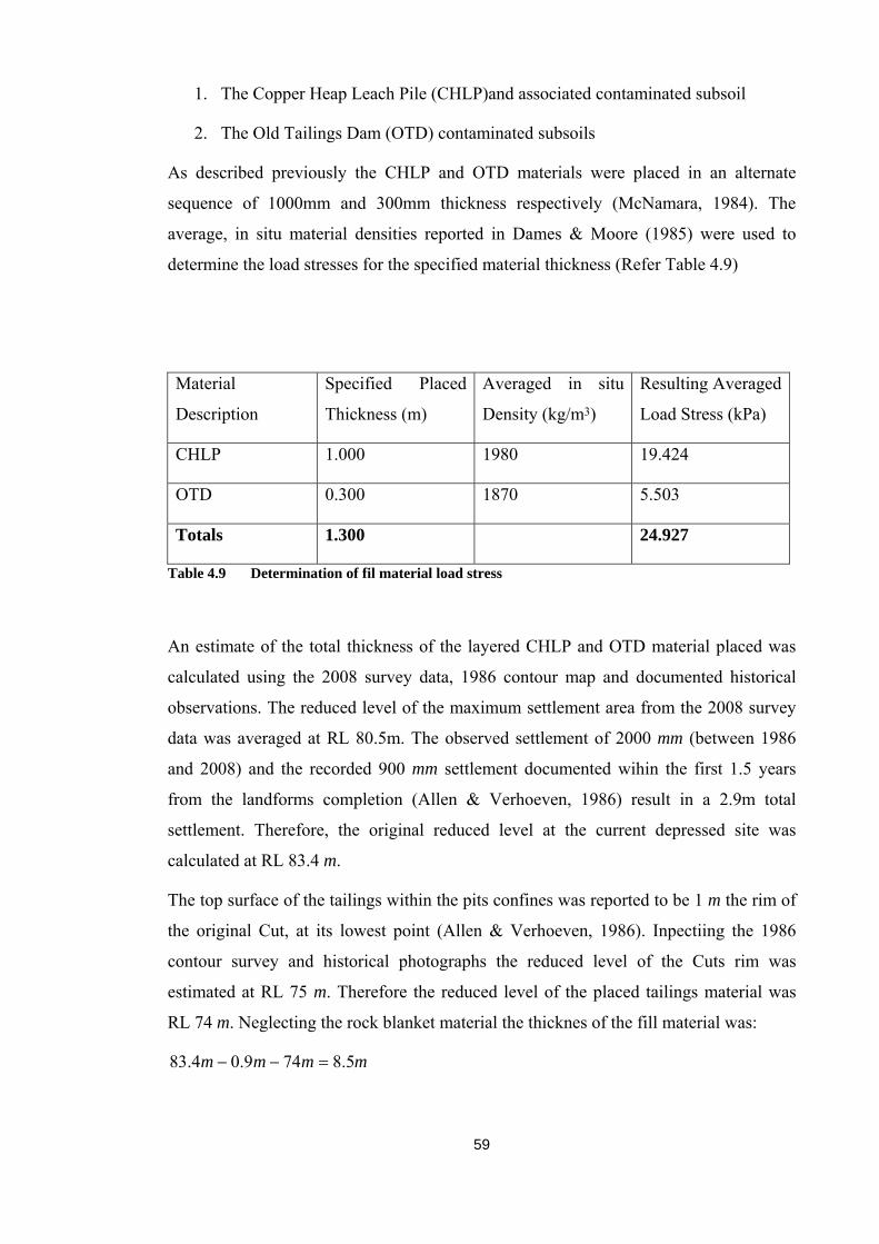
59
1. The Copper Heap Leach Pile (CHLP)and associated contaminated subsoil
2. The Old Tailings Dam (OTD) contaminated subsoils
As described previously the CHLP and OTD materials were placed in an alternate
sequence of 1000mm and 300mm thickness respectively (McNamara, 1984). The
average, in situ material densities reported in Dames & Moore (1985) were used to
determine the load stresses for the specified material thickness (Refer Table 4.9)
Material
Description
Specified Placed
Thickness (m)
Averaged in situ
Density (kg/m3)
Resulting Averaged
Load Stress (kPa)
CHLP 1.000 1980 19.424
OTD 0.300 1870 5.503
Totals 1.300 24.927
Table 4.9 Determination of fil material load stress
An estimate of the total thickness of the layered CHLP and OTD material placed was
calculated using the 2008 survey data, 1986 contour map and documented historical
observations. The reduced level of the maximum settlement area from the 2008 survey
data was averaged at RL 80.5m. The observed settlement of 2000 mm (between 1986
and 2008) and the recorded 900 mm settlement documented wihin the first 1.5 years
from the landforms completion (Allen & Verhoeven, 1986) result in a 2.9m total
settlement. Therefore, the original reduced level at the current depressed site was
calculated at RL 83.4 m.
The top surface of the tailings within the pits confines was reported to be 1 m the rim of
the original Cut, at its lowest point (Allen & Verhoeven, 1986). Inpectiing the 1986
contour survey and historical photographs the reduced level of the Cuts rim was
estimated at RL 75 m. Therefore the reduced level of the placed tailings material was
RL 74 m. Neglecting the rock blanket material the thicknes of the fill material was:
mmmm 5.8749.04.83 =−−
60
The total load stress from the CHLP and OTD material then became:
kPakPamm 984.162927.24
3.15.8
=×
The estimated total applied load stress upon the tailings material was:
kPakPakPa 375.180984.162373.17 =+
4.5.2 Estimate of the tailings thickness
The assumption was made that the Datum used for the reported maximum Cut depth of
47.5 m (Allen & Verhoeven, 1986) coincided with the lower lip of the Cut which gave
the reduced level of the base at:
mRLmm 5.275.4775 =−
Therefore the maximum thickness of the tailings was estimated as 46.5 m
4.6 Consolidation settlement model, results and discussion
Settlement due to one dimensional consolidation was estimate using the numerically
method with constant (Cv) which implies constant values (k) and (mv)
The model is restricted to the area of the largest observed settlement, near to the centre
of the Cut and at the assumed deepest section of the original excavation. As estimated
previously this is the likely site of the finer grained tailings, slime and sludge
components of the tailings material of which a high value of compressibility is assumed.
The finite difference method described previously was applied to the one dimensional
consolidation equation using a Microsoft Office Excel spreadsheet to calculate the
excess pore pressure and settlement. A plot of the settlement variation over the
consolidation time period was produced using model rsults. The model input values
were:

61
Applied instantaneous load stress = 180.375 kPa
Tailings depth = 46m
Consolidation duration = 22 years
The coefficient of consolidation (Cv) was arbitrarily chosen from the data in Table 4.7
Cv = 8.5m2/year
dt = 0.055 years
dz = 1m
Betta = 0.4675 < 0.5
These values were used in the model equation and the value of mv was changed until the
current, estimated total observed settlement value of 2.9 m was returned for the period
of 22 years. A representative portion of the data is included in Appendix D and the plot
of settlement against time is presented in Figure .
The final value of mv was equal to 0.00104 m2/kN, which is comparable to the value
range of normally consolidated alluvial clays in Table 4.1. The permeability coefficient
(k) can be calculated with manipulation of the equation from Terzarghis theory of one
dimensional consolidation:
vwv m
kCγ
=
Taking the unit weight of water as 9.81 kN/m3, the k coefficient is calculated as 0.0867
m/year or 2.75 x 10⁻⁹ m/s and is a plausable value on comparison to those in Table .
The observed maximum settlement of the landform surface after approximately a 1.5
year time lapse from construction completion was reported to be 900mm (Allen &
Verhoeven, 1986). This observed value compared well with the approximate 800mm
settlement value returned by the model for the same elapsed time (Refer Appendix D).
This 100mm settlement difference suggests a reduced pore water dissipation rate in the
model. The plot in Figure 4.6 describes the decreasing rate of settlement over time as
expected. The slope of the curve also suggests that settlement due to consolidation has a
long way to go before excess pore pressures are full dissipated and equilibrium is
achieved (volume change due to consolidation ceaseing).

62
Figure 4.6 Plot of one dimensional consolidation settlement against time.
4.6 Discussion of the model deficiencies
The model and results presented showed that if the all the assumptions and input
parmeters are in fact correct the predicted settlement agrees well with the observed
settlement. However this condition is highly unlikely to exist. In many cases the
predictions of volume change settlement and the rate at which it occurs based on the
above simple theory yields inaccurate results (Mitchell, 1993). The potential for a
reasonable settlement agreement are reduced due to the compounding affect of the
following many reasons.
• The inherent assumptions that form the basis of Terzarghis one dimensional
consolidation equation are not representative of the realistic process;
o The void ratio-effective stress relationship is not linear
o Void ratio decreases with volume change
o Permeability decreases with decreasing void ratio
o Coefficient of volume decrease is not constant with respect to time nor
depth in the layer.
o The tailings material not likely homogenous through the full layer depth

63
o The saturated soil condition may not be the case for the full 22 year time
period
o Soil creep (secondary compression) is not considered
o Self weight of the material within the layer is at no time considered to
contribute to effective pressure through the layer depth.
• Errors associated with the Finite difference equation and Trapezoidal
approximation method.
• Many potentially inaccurate assumptions were made with respect to fill material
thicknesses for determining the constant load stress place on the tailings
• High potential inaccuracy of the tailings thickness estimate and distance to
permeable drainage surface.
• Potential inaccurate assumption of an impervious base and one way drainage
during consolidation as the potential pervious nature of the Cut base, due to the
documented geological fault system was ignored.
• Limited Geotechnical investigation data of the tailings material. Characteristics
for estimating deformation behaviour of the finer saturated material were not
investigated resulting in assumed input values
• Two and three dimensional stress and drainage effects may be substantial.

64
Chapter 5 – Conclusion
The specific objective of the project was not met. The comparison of model predicted
consolidation settlement to the measured actual long term subsidence of the
rehabilitated, Dysons Open Cut at Rum Jungle Mining Lease could not be achieved the
lack of geotechnical data. However several associated outcomes have been achieved.
The settlement of the Dysons rehabilitated landform between the years 1986 and 2008
has been quantified with good accuracy given that actual historical XYZ survey data
could not be found and an existing contour map had to be used. The major
characteristics that will influence the potential instability of a landform constructed
above a layer of impounded tailings are now better understood. Also Terzaghis one
dimensional consolidation model was successfully calibrated using a combination of
field survey to measure settlement and published geotechnical properties. The
knowledge gained from this study could be used for improvement of other mines future
investigations and design of stable capping structures. Further, The investigation
process has identified the areas to which further work is necessary to complete the
project (described in the following section).
65
Chapter 6 - Further work Required
The major limiting factors influencing a realistic comparison of model predicted
settlement to the observed settlement at Dysons is the limited knowledge of the tailings
geotechnical characteristics.
The geotechnical characteristics can be investigated by developing and implementing a
drilling program that recovers relatively undisturbed tailing samples for laboratory
testing. This drilling program has the potential to yield many beneficial outcomes such
as:
• The soil stratum could be mapped quantifying layer depths both in the landform
and the tailings.
• The volume change behaviour of the tailings would be better understood through
laboratory testing of the samples recovered.
• Toxicity analysis’s can be performed on the samples to better understand and
assess the environmental risks existing at the site.
• The process by which further settlement occurs can be determined by installing
piezometers in the bore holes on completion of sampling and pressures monitored.
The excess pore water pressures then may be monitored over an extended period
of time. If the recorded pressures remain relatively constant, futher settlement may
be attributed to secondary compression alone and the consolidation process
completed. The pore pressure information could then be used in developing a more
realistic settlement model.
• Water pressure data could be compared to data from the adjacent bores to
determine the the true flow path boundary coditions.
• Water toxicity could be monitored within the landform and tailings layers via
installed probes and/or a water sampling program.
• Armed with even some of the above outcomes investigations into using or
developing a more accurate settlement model could then commence.

66
Appendices A. Project Specification B. Site Photos and maps C. Tailings material geotechnical data D. Model data results & 2008 Survey Data

67
Appendix A - Project Specification

68
University of Southern Queensland
Faculty of Engineering and Surveying
ENG4111/4112 Research Project Project Specification
For: Richard John Houghton
Topic Assess impact of tailings subsidence on rehabilitated landform erosional stability
Supervisor: Jim Shiau Ken Evans, ERISS Enrolenent: ENG 4111 – S1, D, 2008 ENG 4112 – S2, D, 2008 Project Aim: To estimate the likely extent of post-rehabilitation waste rock
dump settlement as a result of tailings consolidation/subsidence and simulate the effects of settlement on long term erosion using landform evolution modelling.
Specific objectives: Compare the predicted consolidation settlement to the measured actual long term subsidence of the rehabilitated, Dysons' open cut pit at Rum Jungle Mining Lease. If the predicted and actual subsidence rates do not agree an investigation into modifying the prediction model parameters and apply for an agreement with actual measured subsidence will be performed.
Sponsorship: Department of the Environment, Water Heritage and the Arts
Environmental Institute of the Supervising Scientist (ERISS)
Programme:
1. Through the detailed documentation of the rehabilitation of Rum Jungle Mineincluding material characteristics, survey information, engineering design and construction methods a simple theoretical model will be presented to estimate the subsidence of the landform due to consolidation. The adequacy of this model can be tested against the measured actual subsidence that has occurred at this same site. If the theoretical model calculations agree with actual measured subsidence, the model can be said to be of good reliability.
2. A current site level survey will be performed and compared to the rehabilitated, as constructed survey for the total subsidence value. At the time of writing, the location of post site rehabilitation survey data has not been found although the

69
monitoring reports listed above make mention of them being performed. However an as-constructed design diagram is contained in the final rehabilitation report (Allen C & Verhoeven T, June 1986). When these surveys are located it may be possible to determine an actual subsidence rate curve.
3. An attempt will be made to build a relatively simple model to predict the actual settlement at Dysons’ Pit, investigating parameter manipulation such as modifying exponent values.
4. In addition an investigation into commercially available computer models will be undertaken testing for predicted and actual subsidence agreement at Dysons’ Pit.
As Time Permits:
1. Incorporate the results from the above consolidation model to estimate the evolutionary consolidated settlement of the rehabilitated, open cut pit No1, landform at the Ranger Mine which is due to begin rehabilitation in the near future.
2. Extend the application in Part 2 to the rehabilitation of pit No 3 which is currently being mined.
3. Estimate the erosion effects of this evolutionary subsidence stability of the proposed rehabilitated landform on the surrounding catchments.
Agreed:
________________(Student)________________ , _________________(Supervisors)
Examiner/Co-examiner:_________________________________________________

70
Appendix B - Site Photos and maps
B. 1 Location map of the Ranger Uranium Mine (Fourie & Tibbet, 2006)
B. 2 Rum Jungle mine site plan
B. 3 Dysons landform design
B. 4 Dysons Open Cut 1962 taken from Archives of Australia
B. 5 Dysons Open Cut 1958 taken from Archives of Australia
B. 6 Dysons Open Cut 1958 taken from Archives of Australia
B. 7 Dysons landform, evidence of monsoonal scour at site of maximum settlement,
April 2008
B. 8 Dysons landform, evidence of monsoonal scour at site of maximum settlement,
April 2008

71
B. 1 Location map of the Ranger Uranium Mine (Fourie & Tibbet, 2006)

72
B. 2 Rum Jungle mine site plan

73
B. 3 Dysons landform design
B. 4 Dysons Open Cut 1962 taken from Archives of Australia

74
B. 5 Dysons Open Cut 1958 taken from Archives of Australia
B. 6 Dysons Open Cut 1958 taken from Archives of Australia

75
B. 7 Dysons landform, evidence of monsoonal scour at site of maximum settlement, April 2008
B. 8 Dysons landform, evidence of monsoonal scour at site of maximum settlement, April 2008

76
Appendix C - Tailings material geotechnical data
Dysons Open Cut Geotechnical data taken from McNamara, (1984)
C. 1 Dysons Cut soil tesing location plan
C. 2 Dysons existing, in cut tailings Atterberg Limits
C. 3 Dysons existing in cut tailings PSD data
C. 4 Old Tailings Dam PSD data
C. 5 Old Tailings Dam Atterburg Limits
C. 6 Old Tailings Dam Dynamic Penetrometer test results
C. 7 Old Tailings Dam Dynamic Penetrometer test results
C. 8 Dysons Open Cut Dynamic Penetrometer test results
C. 9 Dysons Open Cut Dynamic Penetrometer test results
C. 10 Static cone penetrometer test results
C. 11 Old Tailings Dam in situ shear vane test results

77
C. 1 Dysons Cut soil tesing location plan

78
C. 2 Dysons existing, in cut tailings Atterberg Limits

79
C. 3 Dysons existing in cut tailings PSD data
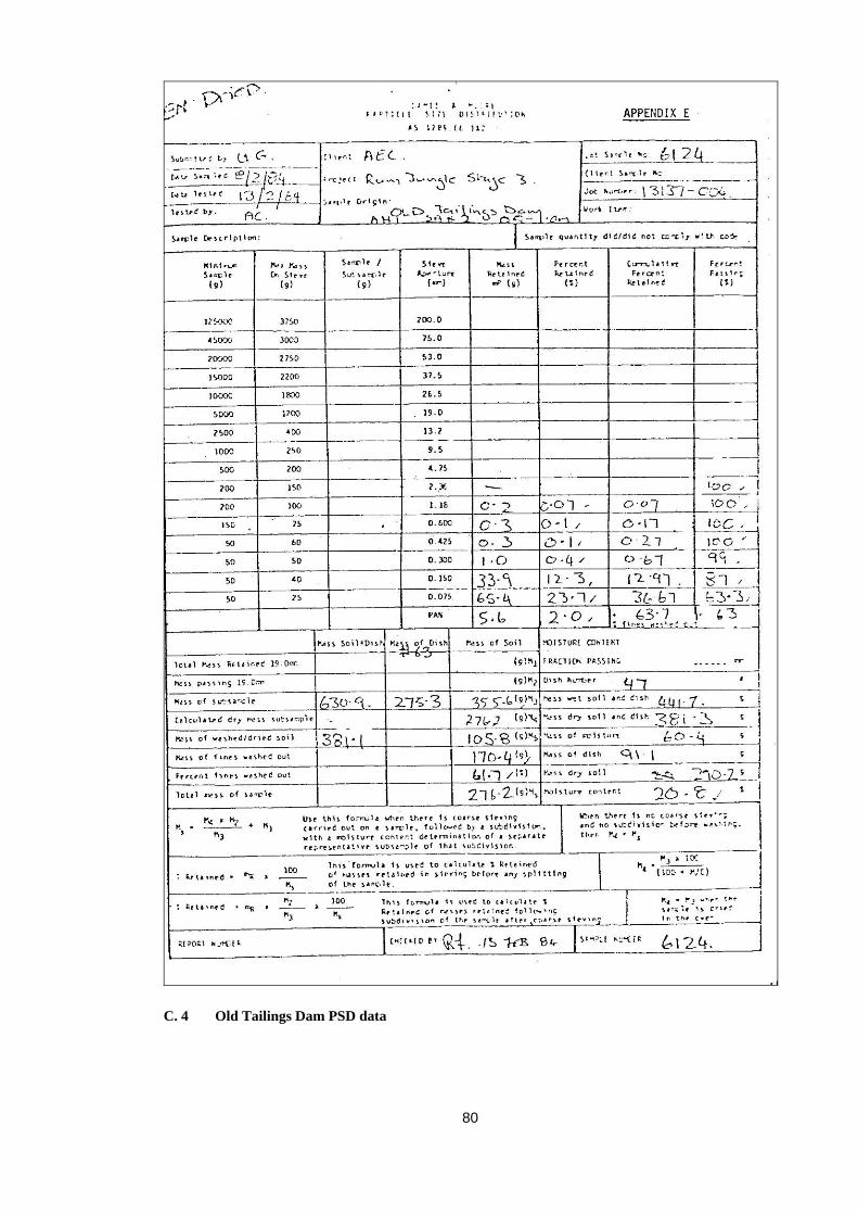
80
C. 4 Old Tailings Dam PSD data
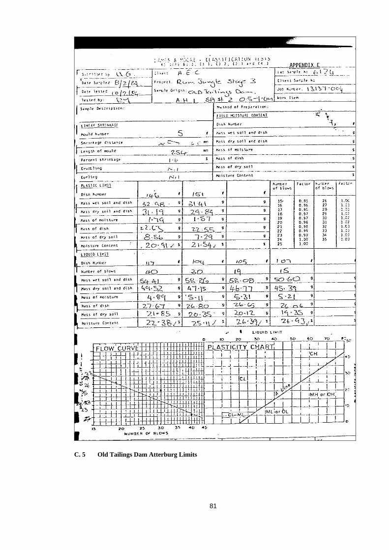
81
C. 5 Old Tailings Dam Atterburg Limits

82
C. 6 Old Tailings Dam Dynamic Penetrometer test results

83
C. 7 Old Tailings Dam Dynamic Penetrometer test results

84
C. 8 Dysons Open Cut Dynamic Penetrometer test results

85
C. 9 Dysons Open Cut Dynamic Penetrometer test results

86
C. 10 Static cone penetrometer test results

87
C. 11 Old Tailings Dam in situ shear vane test results

88
Appendix D – Model data results & 2008 Survey Data
D. 1 Dysons 2008 survey data
D. 2 Dysons 2008 cross section data (parallel to central channel)
D. 3 Dysons 2008 cross section data (orthogonal to central channel)

89
D. 4 Dysons 2008 survey data
Point X Y Z Point X Y Z1 500 4925.63 79.947 58 442.412 4987.91 93.0362 500 4925.63 79.948 59 436.98 4992.97 92.9413 499.97 4925.76 79.699 60 432.438 4997 92.9514 504.488 4913.29 80.03 61 427.933 5001.51 92.9375 504.505 4913.48 79.254 62 426.157 5003.9 92.8956 558.962 4964.9 76.068 63 425.501 5006.56 92.8077 618.188 4990.94 73.448 64 425.209 5008.82 92.7698 397.864 4976.79 95.892 65 424.811 5010.71 92.8079 423.905 4961.73 95.329 66 423.852 5012.93 92.51
10 435.75 4961.28 94.784 67 423.396 5012.41 92.39311 430.506 4971.55 94.699 68 423.993 5010.72 92.61212 425.462 4981.19 94.014 69 424.862 5008.41 92.66713 424.774 4982.44 94.298 70 425.003 5005.2 92.68914 421.942 4986.8 94.321 71 425.663 5002.58 92.6815 419.303 4991.32 94.31 72 427.089 5000.83 92.70416 416.567 4996.91 94.187 73 430.797 4997.24 92.73617 416.472 4997 93.71 74 435.125 4993.31 92.75318 416.373 4997.6 93.83 75 436.674 4992.18 92.79419 416.242 4997.77 94.214 76 440.039 4988.74 92.82120 414.099 5002.53 94.436 77 444.649 4985.5 92.88721 413.366 5000.96 94.183 78 448.234 4984.34 92.91122 415.675 4997.64 94.103 79 453.469 4982.94 93.03423 415.856 4997.4 93.917 80 456.441 4981.44 93.17724 415.822 4996.74 93.863 81 458.213 4979.6 93.37325 416.135 4996.49 93.914 82 460.593 4977.17 93.61426 416.181 4996.43 94.095 83 462.076 4978.3 93.40327 417.877 4992.74 94.125 84 459.825 4981.22 93.0928 419.851 4988.74 94.158 85 456.927 4984.17 92.77429 422.6 4984.31 94.162 86 453.44 4985.33 92.69830 424.394 4981.4 94.065 87 451.075 4985.63 92.68431 426.093 4982.27 93.946 88 447.298 4986.36 92.60132 423.981 4986.01 93.871 89 444.722 4987.56 92.57433 422.169 4988.88 93.88 90 441.93 4989.89 92.49934 420.066 4993.33 93.806 91 439.66 4991.74 92.49735 417.926 4997.46 93.746 92 437.348 4994.03 92.47136 417.765 4997.7 93.553 93 435.009 4996.11 92.46137 417.648 4998.06 93.549 94 432.038 4998.73 92.4538 417.494 4998.36 93.703 95 428.645 5002.35 92.4439 416.305 5001.92 93.64 96 427.388 5004.59 92.33740 416.357 5003.13 93.558 97 426.697 5007.58 92.21541 418.766 5005.23 93.123 98 426.138 5010.58 92.19442 421.603 5001.1 93.124 99 425.447 5013.3 92.01643 421.927 5000.58 93.031 100 428.711 5015.67 91.61444 422.092 5000.3 93.124 101 432.89 5011.14 91.5445 428.745 4992.83 93.101 102 436.643 5006.52 91.58346 435.231 4985.03 93.24 103 440.815 5001.7 91.67447 440.094 4978.6 93.513 104 446.51 4996.36 91.78548 448.472 4972.13 94.066 105 453.08 4991.31 91.92249 451.975 4968.67 94.279 106 458.379 4987.04 92.32350 457.104 4972.45 94.017 107 463.823 4983.61 92.73151 461.824 4975.41 93.694 108 466.764 4981.61 92.98352 461.31 4977.33 93.597 109 468.537 4979.59 93.0453 458.874 4980.05 93.557 110 473.155 4982.73 92.47354 457.028 4981.76 93.393 111 471.078 4985.71 92.50355 454.337 4983.71 93.284 112 470.085 4987.26 92.70856 450.727 4984.68 93.142 113 465.99 4991.16 92.42957 446.429 4985.6 93.056 114 461.868 4995.06 92.153

90
Point X Y Z Point X Y Z 115 456.745 5000.03 91.917 172 455.636 5039.8 88.166116 451.701 5004.77 91.755 173 457.576 5037.33 88.384117 445.962 5010.09 91.598 174 459.537 5035.47 88.523118 441.292 5014.7 91.55 175 464.259 5030.04 88.604119 437.847 5018.44 91.396 176 469.026 5024.38 88.656120 436.891 5020.78 91.015 177 472.5 5020.82 88.776121 437.118 5022.7 90.656 178 475.513 5017.7 88.858122 435.75 5021.9 90.751 179 478.342 5014.47 88.917123 435.545 5019.37 91.095 180 483.287 5009.56 89.145124 436.934 5016.75 91.186 181 488.224 5004.38 89.549125 440.812 5012.87 91.261 182 490.93 5002.31 89.724126 445.722 5007.87 91.298 183 492.686 5002.09 89.648127 450.987 5002.81 91.383 184 495.702 4997.59 89.83128 456.327 4997.93 91.548 185 493.976 5003.01 89.452129 461.819 4992.83 91.819 186 497.694 5005.61 88.92130 466.447 4988.33 92.273 187 495.429 5007.63 88.675131 469.865 4985.7 92.59 188 492.827 5008.74 88.643132 473.136 4986.33 92.273 189 491.389 5009.63 88.601133 470.831 4990.84 91.727 190 488.561 5012.03 88.436134 466.052 4995.71 91.168 191 483.492 5017.76 88.04135 462.899 4999.01 90.932 192 478.155 5023.07 87.927136 456.463 5005.63 90.716 193 471.854 5029.37 87.897137 450.081 5011.83 90.536 194 466.299 5034.33 87.964138 444.338 5017.38 90.39 195 460.947 5039.86 87.952139 439.985 5021.67 90.49 196 460.125 5040.59 88.058140 438.508 5025.07 90.376 197 458.39 5042.36 87.779141 444.915 5030.71 89.409 198 456.527 5040.96 88.035142 450.119 5025.6 89.414 199 458.567 5038.69 88.548143 455.798 5020.29 89.479 200 460.305 5036.8 88.766144 462.655 5014.65 89.602 201 464.433 5032.07 88.89145 467.312 5010.66 89.583 202 468.983 5027.17 88.999146 477.075 5000.42 90.195 203 473.867 5022.03 89.199147 476.441 4998.66 90.394 204 479.878 5015.77 89.398148 476.132 4996.26 90.675 205 485.166 5010.38 89.556149 477.028 4996.65 90.615 206 490.045 5005.53 89.846150 477.825 4997.23 90.543 207 492.682 5003.14 89.772151 477.646 4998.23 90.409 208 493.854 5004.39 89.451152 478.603 5000.35 90.121 209 505.597 5003.48 88.54153 479.458 5002.88 89.809 210 503.738 5008.36 88.257154 479.11 5003.3 89.712 211 500.309 5013.47 87.716155 478.219 5000.78 89.938 212 496.595 5019.26 87.171156 477.214 4999.48 90.079 213 492.184 5025.49 86.796157 477.084 4998.06 90.188 214 488.42 5029.76 86.648158 476.731 4997.09 90.274 215 484.782 5034.47 86.597159 476.266 4996.35 90.386 216 478.306 5041.71 86.542160 481.405 4992.83 91.067 217 472.523 5047.83 86.712161 483.251 4990.34 91.214 218 469.471 5051.03 86.629162 487.434 4993.3 90.717 219 481.388 5061.3 85.375163 485.22 4996.18 90.53 220 484.097 5057.76 85.465164 481.493 5000 90.077 221 488.294 5053.26 85.405165 478.998 5003.86 89.697 222 493.765 5047.16 85.258166 475.11 5008.08 89.425 223 497.702 5042.06 85.308167 472.143 5012.81 89.132 224 502.222 5036.56 85.471168 467.775 5018.95 88.879 225 506.663 5031.48 85.594169 463.178 5024.28 88.72 226 511.168 5026.46 85.781170 457.979 5031.75 88.603 227 516.184 5021.06 86.131171 453.781 5037.92 88.346 228 520.101 5015.83 86.569

91
Point X Y Z Point X Y Z 229 524.801 5013.16 86.304 286 504.101 5079.79 82.941230 523.224 5017.14 86.43 287 513.141 5086.95 82.346231 520.514 5018.21 86.397 288 515.674 5083.36 82.36232 516.831 5023.31 86.042 289 520.038 5077.31 82.416233 510.456 5031.11 85.662 290 521.502 5075.63 82.408234 500.835 5042.64 85.371 291 525.798 5069.12 82.763235 495.782 5048.42 85.283 292 527.295 5066.7 82.858236 490.694 5054.82 85.272 293 531.782 5059.65 83.044237 486.877 5059.22 85.274 294 535.843 5053.6 83.249238 484.392 5062.84 85.254 295 541.234 5046.63 83.438239 486.287 5065.63 85.027 296 545.121 5041.25 83.71240 486.749 5064.37 85.291 297 548.905 5036.06 84.034241 488.044 5061.64 85.547 298 551.746 5031.4 84.34242 490.172 5058.81 85.68 299 553.761 5027.75 84.186243 495.721 5051.81 85.676 300 554.797 5026.13 84.032244 502.026 5044.4 85.779 301 554.654 5031.55 84.203245 508.384 5036.82 85.891 302 554.031 5033.29 84.21246 514.24 5029.71 86.086 303 552.184 5037.49 84.016247 519.08 5023.86 86.352 304 549.845 5043.53 83.652248 522.002 5020.47 86.547 305 547.499 5049.34 83.427249 524.266 5018.56 86.538 306 544.668 5057.12 83.141250 525.919 5017.59 86.176 307 542.523 5062.91 82.947251 528.418 5019.36 85.858 308 540.088 5069.51 82.693252 526.174 5021.67 85.645 309 538.063 5075.07 82.316253 524.801 5024.04 85.372 310 536.545 5081.03 81.967254 521.879 5027.13 85.123 311 534.103 5086.76 81.596255 515.157 5034.43 84.928 312 532.1 5092.5 81.409256 508.849 5042.38 84.716 313 530.086 5096.86 81.161257 502.266 5049.98 84.631 314 529.167 5098.93 81.041258 496.305 5056.78 84.676 315 531.465 5100.5 80.998259 490.774 5063.72 84.73 316 532.348 5098.46 81.446260 487.736 5066.52 84.808 317 533.283 5096.55 81.692261 495.664 5071.85 83.983 318 534.987 5092.26 81.799262 498.553 5068.33 83.984 319 536.571 5087.54 81.975263 502.522 5063.91 83.906 320 538.398 5082.47 82.267264 507.215 5058.45 84.057 321 540.152 5077.39 82.684265 512.678 5052.3 84.034 322 542.195 5071.61 83.091266 517.379 5046.77 84.072 323 543.927 5066.32 83.381267 521.302 5042 84.28 324 546.369 5060.07 83.588268 525.879 5036.99 84.26 325 548.662 5053.87 83.821269 530.343 5032.96 84.323 326 551.113 5047.67 84.004270 533.308 5029.32 84.597 327 553.572 5041.33 84.21271 536.021 5024.66 85.042 328 555.844 5035.96 84.483272 537.578 5021.86 85.183 329 556.441 5034.29 84.489273 538.93 5019.19 85.136 330 556.863 5033.14 84.355274 547.626 5024.15 84.501 331 557.199 5032.34 84.071275 545.882 5026.71 84.642 332 558.65 5029.05 83.917276 543.904 5029.36 84.551 333 559.203 5034.13 83.988277 538.817 5036.52 83.902 334 558.718 5035.41 84.078278 534.896 5042.35 83.628 335 556.777 5039.34 83.93279 532.714 5045.14 83.645 336 555.48 5043.11 83.725280 524.445 5054.83 83.415 337 552.929 5050.03 83.468281 519.372 5061.14 83.382 338 551.261 5054.07 83.293282 516.199 5065.05 83.247 339 549.775 5058.32 83.092283 511.267 5070.99 83.096 340 548.179 5062.9 82.894284 507.718 5075.06 83.094 341 545.342 5069.95 82.67285 505.297 5078.05 83.045 342 544.477 5072.99 82.464

92
Point X Y Z Point X Y Z 343 543.117 5077.21 82.178 400 587.97 5073.38 82.47344 541.402 5081.85 81.795 401 585.253 5079.88 82.329345 539.71 5086.33 81.526 402 583.575 5084.16 82.298346 538.003 5090.49 81.317 403 580.736 5089.68 81.963347 536.897 5094.5 81.14 404 578.658 5094.2 81.704348 535.411 5098.1 81.026 405 576.302 5098.84 81.34349 534.005 5100.99 80.922 406 573.556 5103.98 81.051350 533.401 5102.12 80.732 407 570.783 5108.35 80.834351 540.097 5106.33 80.444 408 567.41 5112.9 80.566352 540.962 5104.8 80.569 409 565.939 5116.37 80.304353 543.217 5100.02 80.819 410 570.686 5116.95 80.387354 545.002 5095.7 81.035 411 572.933 5117.32 80.55355 547.414 5091.37 81.247 412 573.235 5114.81 80.582356 550.339 5086.34 81.62 413 575.341 5112.07 80.853357 552.507 5080.62 82.086 414 577.748 5106.9 80.987358 554.959 5074.9 82.482 415 580.66 5101.48 81.222359 557.657 5069.51 82.758 416 582.431 5097.17 81.439360 560.395 5064.01 82.937 417 585.14 5092.73 81.756361 562.974 5058.19 83.15 418 587.334 5088.24 82.083362 565.329 5052.61 83.311 419 590.296 5083.24 82.191363 567.911 5047.31 83.472 420 593.119 5077.44 82.304364 570.226 5043.1 83.583 421 595.619 5072.41 82.433365 572.146 5040.04 83.54 422 598.064 5067.97 82.486366 581.196 5044.88 83.216 423 602.624 5063.43 82.356367 579.213 5047.5 83.348 424 601.021 5067.41 82.439368 577.57 5050.79 83.295 425 598.359 5070.97 82.715369 575.465 5056.87 83.194 426 595.992 5075.69 82.749370 572.811 5063.31 82.97 427 593.588 5080.65 82.668371 569.862 5070.46 82.825 428 591.488 5085.3 82.591372 567.109 5076.23 82.631 429 589.129 5089.83 82.428373 564.886 5082.16 82.256 430 586.709 5094.58 82.256374 562.088 5087.89 81.793 431 583.994 5099.62 81.928375 559.339 5093.49 81.408 432 581.274 5104.33 81.644376 556.803 5099.29 81.036 433 578.799 5109.22 81.422377 554.285 5104.83 80.679 434 575.908 5114.94 81.154378 552.567 5109.15 80.361 435 574.891 5116.77 80.851379 550.968 5111.91 80.15 436 574.987 5118.01 80.415380 559.827 5115.22 80.142 437 577.792 5118.27 80.328381 561.551 5110.53 80.552 438 578.068 5115.26 80.686382 563.931 5105.65 80.86 439 580.056 5112.24 80.779383 566.542 5100.46 81.15 440 581.771 5109.22 80.799384 569.91 5094.98 81.492 441 584.276 5104.56 80.987385 571.985 5090.05 81.816 442 586.785 5099.67 81.302386 572.432 5089.07 81.97 443 589.939 5094.28 81.548387 573.913 5086.07 82.176 444 592.568 5089.07 81.804388 575.617 5080.99 82.399 445 595.376 5083.58 81.964389 577.974 5075.64 82.569 446 597.524 5078.54 82.074390 580.726 5070.16 82.684 447 599.602 5073.55 82.244391 583.656 5064.74 82.884 448 601.875 5068.82 82.31392 585.197 5061.48 82.996 449 604.231 5065.78 82.272393 588.152 5056.86 83.02 450 611.75 5070.43 81.786394 589.599 5054.63 82.988 451 609.595 5073.34 81.926395 591.118 5052.53 82.827 452 606.806 5078.46 81.777396 596.959 5058.02 82.629 453 603.796 5083.74 81.629397 595.648 5059.73 82.706 454 600.733 5088.94 81.47398 593.992 5061.87 82.746 455 597.556 5094.15 81.35399 590.682 5067.4 82.653 456 594.61 5099.95 81.082

93
Point X Y Z Point X Y Z 457 591.89 5105.08 80.844 514 639.983 5105.54 78.939458 589.544 5109.86 80.692 515 641.197 5101.95 78.946459 587.323 5114.93 80.581 516 642.852 5098.29 78.876460 586.156 5118.58 80.468 517 645.377 5094.23 78.75461 597.212 5118.26 80.313 518 652.889 5097.7 78.187462 599.058 5114.26 80.473 519 651.588 5101.57 78.401463 601.72 5108.77 80.575 520 649.921 5104.68 78.494464 604.416 5103.14 80.701 521 648.337 5108.63 78.523465 607.926 5098.03 80.735 522 646.69 5114.41 78.409466 611.052 5093.17 80.784 523 646.286 5115.96 78.478467 614.076 5089.04 80.806 524 654.471 5115.12 78.098468 616.844 5083.99 81.012 525 655.429 5110.73 78.156469 620.746 5078.59 81.051 526 656.566 5106.9 78.22470 626.79 5081.68 80.43 527 657.679 5103.8 78.151471 625.403 5084.95 80.489 528 658.681 5100.87 78.04472 623.562 5088.92 80.258 529 666.822 5102.17 77.682473 621.488 5093.72 80.141 530 665.53 5106.03 77.786474 619.003 5098.72 80.129 531 664.851 5110.5 77.773475 616.752 5103.92 80.103 532 664.116 5114.62 77.664476 615.169 5107.18 80.077 533 649.366 5122.78 78.775477 613.115 5110.35 80.095 534 653.461 5129.71 78.823478 610.633 5116.51 80.138 535 656.865 5136.52 79.151479 610.466 5117.77 80.017 536 660.283 5142.64 79.31480 619.353 5116.89 79.699 537 662.017 5146.34 79.145481 619.848 5114.16 79.764 538 663.613 5149.85 78.69482 621.061 5108.89 79.778 539 658.048 5144.73 79.558483 622.698 5102.43 79.831 540 657.19 5142.82 80.392484 624.046 5096.36 79.946 541 656.452 5140.83 80.252485 625.543 5090.43 80.159 542 653.646 5136.38 79.845486 626.983 5088.42 80.253 543 650.891 5131.57 79.592487 627.316 5086.28 80.394 544 647.375 5125.16 79.51488 629.279 5089.85 80.589 545 647.108 5123.99 79.349489 628.917 5094.75 80.488 546 646.97 5122.58 78.741490 628.296 5100.73 80.244 547 644.484 5123.52 78.929491 627.315 5106.8 80.165 548 645.392 5126.25 79.062492 627.063 5110.61 80.093 549 648.401 5130.66 79.217493 626.651 5113.55 80.164 550 651.206 5135.25 79.402494 626.626 5114.97 79.976 551 654.156 5140.89 79.57495 626.68 5115.94 79.645 552 656.326 5144.92 79.613496 626.691 5117.37 79.147 553 658.463 5149.32 79.278497 624.35 5117.22 79.423 554 659.791 5151.86 78.741498 623.949 5115.62 79.593 555 652.695 5157.32 79.194499 624.324 5113.22 79.654 556 649.831 5154.45 79.887500 625.301 5109.05 79.678 557 647.835 5151.31 79.988501 625.68 5105.7 79.725 558 645.688 5147.39 80.12502 626.187 5101.27 79.817 559 642.826 5142.14 79.959503 626.73 5096.52 79.924 560 639.075 5135.63 79.785504 627.314 5091.46 80.109 561 636.187 5130.17 79.451505 633.075 5088.13 79.79 562 633.513 5124.62 79.336506 632.285 5092.3 79.72 563 633.169 5123.48 79.358507 631.644 5098.24 79.536 564 624.389 5123.98 79.666508 630.827 5104.64 79.425 565 627.012 5131.37 79.844509 630.199 5110.92 79.364 566 629.79 5137.48 80.226510 629.906 5115.88 79.201 567 632.519 5144.19 80.474511 629.933 5116.98 79.093 568 636.155 5149.9 80.569512 638.477 5116.16 78.762 569 638.426 5154.58 80.709513 639.203 5111.17 78.827 570 639.762 5157.1 80.656

94
Point X Y Z Point X Y Z 571 640.83 5158.54 80.371 628 600.566 5190.2 83.793572 643.134 5161.88 80.428 629 598.745 5188.92 83.867573 645.669 5165.91 79.524 630 593.979 5185.33 83.743574 639.136 5172.2 79.778 631 588.535 5182.1 83.692575 635.485 5167.7 81.001 632 581.29 5177.38 83.521576 632.623 5164.27 81.039 633 576.348 5173.38 83.279577 632.028 5163.59 81.276 634 571.878 5170.13 82.999578 628.745 5159.05 81.257 635 568.331 5167.21 82.655579 625.144 5153.12 81.122 636 563.787 5163.08 82.044580 621.51 5147.35 80.981 637 560.35 5159.89 81.554581 618.927 5143.07 80.735 638 557.239 5155.66 81.273582 616.801 5137.04 80.492 639 553.882 5151.22 80.878583 614.767 5130.66 80.207 640 549.239 5145.65 80.576584 612.843 5124.34 80.061 641 545.324 5140.3 80.342585 605.852 5124.67 80.17 642 542.405 5135.04 80.323586 607.999 5132.99 80.404 643 540.395 5128.87 80.213587 610.576 5140.69 80.762 644 538.683 5122.09 80.214588 611.991 5146.52 81.142 645 536.979 5117.36 80.198589 614.696 5155.38 81.659 646 535.567 5113.96 80.158590 616.57 5161.79 81.81 647 535.736 5111.84 80.156591 619.439 5169.48 82.043 648 538.493 5112.89 79.881592 621.491 5173.25 82.01 649 540.542 5117.59 79.864593 625.109 5178.76 81.713 650 542.014 5123.84 79.705594 626.391 5181.44 81.152 651 543.202 5128.85 79.77595 628.369 5184.19 80.256 652 545.348 5133.99 79.803596 622.564 5189.27 80.746 653 549.036 5139.66 79.927597 620.084 5186.48 81.756 654 553.451 5145.47 80.241598 617.601 5183.46 82.307 655 557.95 5150.21 80.54599 615.326 5181.03 82.359 656 562.729 5154.85 80.966600 614.149 5179.77 82.595 657 567.987 5159.54 81.543601 611.456 5176.47 82.668 658 573.18 5163.91 82.16602 608.578 5171.79 82.384 659 578.112 5168.46 82.632603 605.304 5166.07 82.247 660 583.298 5172.89 83.026604 602.536 5160.61 82.016 661 587.328 5176.01 83.29605 599.408 5154.91 81.575 662 593.075 5179.53 83.32606 595.991 5149.08 81.007 663 598.251 5182.91 83.288607 593.985 5143.07 80.606 664 601.913 5186.25 83.565608 591.891 5136.75 80.191 665 604.013 5184.24 83.264609 590.676 5131.07 80.038 666 601.471 5181.8 83.11610 589.466 5125.92 80.054 667 598.432 5178.2 83.07611 589.382 5125.1 79.982 668 595.824 5175.47 82.982612 582.927 5125.19 79.9 669 592.368 5171.53 82.798613 585.223 5130.83 79.859 670 589.902 5168.76 82.607614 587.7 5137.49 80.036 671 587.08 5165.73 82.315615 590.431 5144.07 80.487 672 584.253 5162.49 81.966616 593.191 5151.24 81.061 673 581.48 5159.13 81.563617 596.166 5158.43 81.74 674 578.531 5155.99 81.106618 598.912 5165.06 82.316 675 575.693 5152.48 80.568619 601.567 5172.01 82.58 676 572.161 5148.66 80.149620 604.779 5180.2 82.839 677 569.794 5144.21 79.856621 606.8 5184.5 83.148 678 569.786 5144.19 79.857622 609.353 5189.04 83.135 679 565.75 5139.98 79.678623 610.784 5192.43 83.016 680 562.315 5135.59 79.583624 612.062 5198.39 81.955 681 557.912 5130.69 79.551625 607.007 5201.96 82.434 682 555.114 5126.13 79.551626 605.024 5198.56 83.442 683 552.764 5121.05 79.554627 602.949 5194.74 83.838 684 551.903 5119.06 79.508

95
Point X Y Z Point X Y Z 685 545.604 5120.59 79.607 742 500 4925.68 79.871686 548.117 5126.13 79.625 743 504.67 4913.38 80.036687 550.652 5131.5 79.578 744 500.19 4925.57 79.661688 553.471 5136.98 79.679 745 559.014 4964.99 76.07689 555.995 5143.08 79.876 746 558.916 4965.07 75.945690 559.052 5149.25 80.381 747 500.076 4925.63 79.954691 562.219 5154.71 80.988 748 500.054 4925.75 79.706692 500 4925.63 79.955 749 504.289 5002.91 88.725693 499.961 4925.74 79.711 750 397.89 4976.72 95.883694 500.007 4925.63 79.95 751 404.828 4971.67 95.724695 499.997 4925.75 79.709 752 411.913 4967.06 95.571696 650.223 5022.21 73.85 753 419.575 4962.86 95.37697 609.875 5122.02 79.201 754 424.323 4961.2 95.273698 609.725 5120.16 79.162 755 430.481 4960.09 94.994699 604.624 5120.51 79.295 756 430.85 4965.07 95.017700 604.502 5122.51 79.295 757 423.657 4966.54 95.258701 599.235 5122.65 79.404 758 414.905 4968.88 95.532702 598.905 5120.75 79.302 759 409.333 4973.08 95.657703 592.94 5120.84 79.349 760 401.78 4980.26 95.765704 592.552 5122.94 79.331 761 397.317 4983.21 95.941705 586.222 5122.83 79.259 762 391.926 4990.14 95.931706 586.09 5120.93 79.296 763 386.302 4998.23 95.961707 578.087 5120.8 79.252 764 382.013 5007.04 95.893708 577.609 5122.82 79.154 765 378.459 5016.95 95.8709 571.346 5122.38 79.081 766 376.607 5025.77 95.727710 571.395 5120 79.225 767 372.689 5035.32 95.673711 564.819 5119.15 79.134 768 371.861 5027.67 95.716712 564.114 5121.23 79.077 769 372.496 5019.59 95.725713 559.026 5119.8 79.015 770 373.841 5011.26 95.748714 559.312 5117.76 79.097 771 377.368 5002.56 95.696715 555.301 5116.57 79.011 772 380.687 4995.65 95.899716 554.851 5118.23 78.929 773 384.117 4989.6 95.919717 550.21 5116.35 79.018 774 389.316 4983.65 95.882718 550.698 5114.68 79.016 775 395.309 4978.02 95.853719 547.071 5113 79.06 776 394.745 4981.72 95.971720 546.349 5114.49 79.063 777 390.294 4987.2 96.013721 540.949 5111.82 79.26 778 385.825 4993.01 96.039722 541.298 5109.86 79.279 779 383.382 5001.49 95.946723 534.772 5108.22 79.48 780 380.079 5021.98 95.616724 535.435 5106.33 79.485 781 384.222 5015.11 95.639725 529.785 5102.47 79.951 782 389.531 5007.48 95.56726 528.724 5103.87 80.003 783 393.952 5000.25 95.548727 528.725 5103.88 80.003 784 398.642 4993.28 95.518728 523.543 5100.06 80.501 785 403.23 4988.04 95.403729 524.449 5098.49 80.495 786 407.959 4982.42 95.35730 518.091 5093.72 80.956 787 412.768 4977.56 95.279731 516.799 5095.14 81.053 788 411.022 4978.6 95.384732 510.189 5089.66 81.549 789 409.424 4981.46 95.371733 511.002 5088.01 81.576 790 408.275 4984.55 95.306734 504.227 5082.49 82.115 791 405.782 4988.21 95.228735 502.814 5083.84 82.19 792 405.346 4989.15 95.148736 496.623 5078.99 82.778 793 405.584 4989.32 94.846737 497.67 5077.38 82.761 794 406.35 4989.74 94.674738 490.165 5071.25 83.528 795 407.768 4990.5 94.767739 488.457 5072.49 83.546 796 409.05 4991.57 94.601740 481.132 5066.62 84.321 797 410.128 4992.86 94.514741 482.27 5065.08 84.31 798 410.791 4992.19 94.542

96
Point X Y Z Point X Y Z 799 409.644 4993.49 94.557 856 384.776 5026.62 95.278800 409.877 4993.12 94.504 857 380.34 5030.79 95.458801 410.301 4992.39 94.522 858 377.046 5033.62 95.566802 409.126 4991.31 94.661 859 374.312 5034.78 95.64803 409.269 4991.15 94.734 860 375.13 5038.43 95.545804 408.383 4991.95 94.759 861 377.135 5036.88 95.511805 407.96 4992.38 94.794 862 380.402 5034.86 95.359806 406.909 4993.55 94.81 863 384.15 5031.17 95.166807 405.907 4994.84 95.242 864 387.464 5027.2 94.991808 406.325 4993.35 94.904 865 390.823 5022.32 94.857809 407.045 4991.97 94.872 866 394.091 5017.32 94.8810 407.584 4991.12 94.842 867 398.053 5011.84 94.72811 407.96 4990.19 94.865 868 401.487 5007.29 94.699812 409.07 4988.45 94.912 869 405.307 5002.83 94.66813 411.201 4984.97 94.909 870 407.87 5005.13 94.382814 413.062 4981.01 95.021 871 405.615 5008.02 94.36815 412.096 4978.76 95.488 872 402.624 5012.85 94.313816 411.122 4980.44 95.553 873 399.288 5018.03 94.31817 409.909 4982.95 95.504 874 396.806 5023 94.374818 408.559 4985.83 95.398 875 394.201 5028.4 94.421819 406.627 4989.28 95.33 876 391.577 5034.27 94.533820 406.084 4990.06 95.184 877 389.071 5039.99 94.658821 405.894 4990.51 95.38 878 386.538 5043.45 94.874822 405.326 4991.6 95.541 879 383.5 5046.58 95.068823 404.518 4993.21 95.543 880 379.183 5050.77 95.103824 403.801 4994.28 95.23 881 375.518 5053.94 95.198825 403.102 4992.97 95.279 882 378.293 5059.2 95.112826 404.589 4990.41 95.245 883 383.039 5054.73 94.89827 402.587 4995.87 95.267 884 386.829 5050.34 94.754828 400.653 4997.87 95.295 885 389.242 5047.52 94.647829 401.672 4998.57 95.56 886 392.91 5043.27 94.264830 398.925 5000.18 95.338 887 392.295 5042.45 94.403831 397.024 5003.26 95.347 888 394.457 5037.6 94.361832 393.419 5008.28 95.391 889 396.751 5033.41 94.245833 390.207 5013.29 95.391 890 398.263 5029.53 94.167834 386.988 5018.4 95.444 891 399.52 5025.27 94.201835 383.519 5023.62 95.523 892 401.618 5021.26 94.186836 381.271 5026.51 95.553 893 405.317 5014.97 94.138837 377.985 5029.53 95.612 894 408.863 5009.74 94.089838 375.362 5031.95 95.701 895 411.173 5007.04 94.082839 374.613 5033.84 95.761 896 411.847 5007.76 94.382840 376.072 5032.68 95.751 897 409.86 5009.87 94.473841 378.827 5030.37 95.706 898 408.338 5011.68 94.355842 381.974 5027.17 95.691 899 406.45 5014.93 94.271843 384.109 5024.74 95.686 900 403.693 5019.86 94.304844 386.701 5020.84 95.641 901 400.915 5024.89 94.407845 389.477 5016.55 95.563 902 398.667 5030.78 94.278846 392.088 5012.08 95.533 903 397.226 5033.85 94.329847 394.393 5008.54 95.57 904 394.97 5038.63 94.442848 396.986 5004.93 95.578 905 393.617 5041.5 94.57849 399.016 5001.9 95.512 906 394.704 5043 94.053850 402.62 5000.56 94.954 907 396.167 5039.07 93.905851 400.51 5002.63 95.035 908 397.96 5035.21 93.848852 397.841 5005.99 95.098 909 400.18 5030.01 93.86853 394.334 5011.35 95.075 910 402.468 5024.51 93.887854 390.731 5016.92 95.108 911 405.643 5018.67 93.842855 387.882 5022.01 95.148 912 407.741 5015.28 93.844

97
Point X Y Z Point X Y Z 913 410.092 5011.89 93.783 970 425.97 5033.02 91.3914 412.699 5009.27 93.599 971 423.687 5038.75 91.345915 417.358 5013.43 92.879 972 420.211 5046.74 91.42916 414.21 5018.21 92.947 973 419.237 5049.73 91.496917 411.198 5023.56 93.066 974 415.285 5055.62 91.604918 408.584 5028.77 93.075 975 412.956 5061.47 91.737919 405.759 5034.35 93.117 976 410.792 5067.44 91.935920 402.677 5039.81 93.234 977 408.225 5072.92 92.131921 399.923 5044.56 93.409 978 404.774 5078.55 92.467922 397.185 5049.6 93.702 979 401.699 5083.16 92.741923 394.314 5054.55 93.915 980 400.233 5083.29 93.175924 391.433 5058.7 94.193 981 408.175 5089.38 92.374925 389.569 5061.37 94.299 982 406.415 5091.15 92.835926 385.738 5065.45 94.527 983 408.868 5084.98 92.147927 384.698 5066.58 94.851 984 411.209 5080.23 91.943928 388.793 5070.78 94.483 985 414.088 5076.13 91.87929 389.802 5070.09 94.076 986 415.441 5070.5 91.779930 393.177 5067.11 93.702 987 414.08 5070.07 91.743931 396.007 5063.11 93.553 988 416.927 5064.61 91.66932 400.477 5056.21 93.26 989 415.806 5064.4 91.631933 403.358 5051.61 92.939 990 418.401 5058.19 91.508934 406.974 5046.08 92.612 991 416.484 5057.51 91.508935 409.781 5041.62 92.548 992 420.589 5052.58 91.439936 413.631 5035.52 92.399 993 419.622 5052.47 91.421937 417.097 5030.05 92.38 994 422.834 5047.24 91.392938 419.015 5025.03 92.374 995 421.682 5046.94 91.392939 420.205 5021.2 92.351 996 424.855 5041.94 91.321940 421.36 5018.73 92.313 997 427.278 5036.38 91.303941 420.268 5016.51 92.454 998 428.647 5032.58 91.266942 417.313 5021.42 92.514 999 431.082 5027.78 91.017943 414.947 5027.28 92.586 1000 432.297 5028.67 90.747944 411.652 5033.86 92.553 1001 431.087 5030.14 91.212945 408.367 5040.14 92.678 1002 430.267 5032.84 91.45946 406.451 5045.53 92.682 1003 427.814 5038.35 91.564947 408.927 5046.76 92.45 1004 424.938 5045.06 91.542948 409.371 5045.44 92.731 1005 422.414 5051.99 91.7949 410.892 5041.85 92.778 1006 420.01 5059.95 91.876950 414.281 5036.51 92.598 1007 418.117 5066.92 92.009951 416.897 5032.23 92.549 1008 416.48 5074.31 92.155952 418.694 5028.73 92.478 1009 415.038 5081.67 92.244953 420.458 5022.99 92.455 1010 414.342 5086.24 92.219954 422.258 5019.05 92.456 1011 414.327 5089.49 91.993955 422.835 5020.54 92.002 1012 413.597 5094.08 91.748956 421.577 5024.52 92.001 1013 413.398 5094.43 91.967957 419.751 5029.41 92.046 1014 416.09 5095.76 91.541958 416.879 5034.72 92.062 1015 417.125 5090.93 91.458959 414.422 5038.82 92.146 1016 417.807 5086.04 91.297960 411.58 5043.53 92.258 1017 419.257 5077.82 91.131961 410.195 5046.95 92.298 1018 421.041 5070.09 90.835962 412.078 5047.87 92.078 1019 423.333 5061.64 90.688963 415.137 5042.64 91.954 1020 425.311 5053.11 90.732964 417.966 5037.64 91.812 1021 428.319 5045.43 90.568965 421.195 5032.02 91.705 1022 431.767 5038.72 90.481966 423.31 5026.13 91.675 1023 432.769 5036.2 90.478967 424.757 5022.9 91.646 1024 433.593 5031.95 90.559968 429.224 5026.11 91.121 1025 434.917 5030.55 90.379969 427.365 5029.31 91.262 1026 442.751 5037.28 89.229

98
Point X Y Z Point X Y Z 1027 440.825 5042.34 89.336 1084 462.502 5132.5 87.2641028 438.331 5049.52 89.402 1085 461.479 5133.97 87.4241029 435.201 5058.36 89.514 1086 460.283 5135.84 87.8921030 432.649 5066.79 89.67 1087 462.988 5127.98 87.2831031 429.951 5076.55 89.807 1088 463.672 5124.74 87.061032 426.997 5085.77 90.303 1089 464.089 5120.57 86.7171033 423.911 5094.54 90.646 1090 464.334 5113.52 86.4811034 422.213 5097.5 90.812 1091 464.537 5104.85 86.5331035 421.071 5099.43 91.13 1092 463.981 5095.59 86.721036 420.268 5100.52 91.644 1093 464.48 5086.97 86.7061037 432.045 5108.16 89.879 1094 465.498 5076.35 86.4541038 431.03 5110.2 90.353 1095 466.812 5067.72 86.3841039 435.904 5104.1 89.596 1096 469.038 5059.98 86.2851040 438.336 5096.07 89.296 1097 478.121 5067.15 85.3821041 440.362 5087.08 88.976 1098 477.293 5076.6 85.3911042 443.064 5076.88 88.759 1099 476.288 5087.19 85.3831043 445.35 5066.55 88.453 1100 475.196 5097.11 85.5111044 448.591 5056.5 88.226 1101 475.339 5104.38 85.4171045 451.619 5050.45 88.144 1102 474.548 5112.19 85.4341046 453.894 5047.02 87.877 1103 473.379 5119.7 85.6161047 456.557 5049.46 87.519 1104 473.176 5126.2 85.8791048 454.71 5053.19 87.819 1105 472.685 5131.42 86.4251049 452.705 5061.18 87.757 1106 472.02 5135.23 86.6181050 451.33 5070.51 87.805 1107 469.861 5140.35 86.6261051 450.4 5081.51 87.958 1108 469.133 5142.39 87.1231052 449.747 5089.93 88.124 1109 477.466 5151.28 86.5791053 448.428 5099.42 88.264 1110 477.831 5148.84 86.1641054 447.432 5107.12 88.365 1111 478.993 5142.57 86.1311055 447.409 5111.78 88.437 1112 479.782 5136.75 86.0841056 447.406 5116.53 88.638 1113 481.083 5129.2 85.7091057 445.9 5121.35 88.781 1114 483.332 5129.24 85.6571058 444.683 5122.83 89.283 1115 481.84 5135.38 85.9471059 448.427 5125.04 88.608 1116 483.105 5122.95 85.4791060 447.992 5126.07 89.117 1117 479.753 5122.1 85.4881061 450.768 5120.71 88.5 1118 481.452 5113.05 85.2031062 451.058 5117.33 88.431 1119 484.792 5113.38 85.0561063 451.488 5110.29 88.293 1120 482.56 5104.27 84.9981064 451.771 5101.26 88.227 1121 483.797 5094.51 84.7471065 452.356 5091.72 88.129 1122 485.163 5083.96 84.6511066 452.983 5082.43 87.986 1123 486.236 5076.88 84.611067 453.906 5074.4 87.847 1124 486.703 5074.25 84.5591068 455.388 5065.48 87.677 1125 492.698 5079.33 84.0131069 456.403 5059.55 87.639 1126 492.27 5082.55 84.1121070 457.388 5054.52 87.57 1127 491.055 5088.13 84.1561071 458.184 5051.02 87.402 1128 489.872 5095.76 84.2271072 462.547 5054.46 86.955 1129 490.109 5103.74 84.3731073 463.278 5057.8 86.832 1130 489.925 5111.3 84.7541074 460.657 5058.47 87.1 1131 487.261 5110.91 84.7811075 459.79 5064.59 87.075 1132 486.73 5116.86 85.0891076 458.676 5073.29 87.185 1133 489.543 5116.96 85.1391077 457.588 5083.62 87.366 1134 489.393 5124.36 85.361078 456.934 5092.85 87.489 1135 486.424 5124.17 85.3141079 456.758 5102.43 87.458 1136 486.457 5130.59 85.4441080 456.331 5111.75 87.483 1137 489.399 5130.65 85.4981081 456.041 5119.29 87.702 1138 489.206 5139.09 85.5611082 455.567 5122.9 87.927 1139 485.206 5138.65 85.6411083 453.267 5129.64 88.17 1140 483.976 5146.51 85.756
99
Point X Y Z Point X Y Z 1141 489.143 5147.56 85.589 1198 498.891 5088.87 83.3741142 489.7 5155.41 85.66 1199 500.664 5085.25 83.1061143 485.437 5152.97 85.774 1200 502.014 5086.12 83.2531144 483.579 5157.48 85.815 1201 501.53 5086.69 83.511145 482.413 5159.75 86.254 1202 500.161 5089.7 83.61146 489.364 5160.13 85.698 1203 499.038 5095.28 83.7341147 485.36 5161.57 85.875 1204 498.554 5101.76 83.841148 486.715 5164.41 85.728 1205 500.271 5108.72 84.0381149 490.306 5162.6 85.641 1206 502.689 5114.58 84.1591150 492.743 5165.76 85.406 1207 501.732 5114.96 83.981151 491.483 5163.12 85.651 1208 504.022 5119.05 83.9911152 490.955 5160.53 85.865 1209 504.847 5118.74 84.131153 491.078 5154.69 85.989 1210 507.05 5125.2 84.1151154 491.212 5148.41 85.993 1211 506.064 5125.48 84.0261155 491.366 5139.08 85.965 1212 508.76 5132.14 84.0421156 491.571 5132.35 85.981 1213 509.549 5131.99 84.1171157 491.667 5124.75 85.862 1214 510.96 5136.44 84.0381158 491.788 5118.17 85.704 1215 510.206 5136.74 83.9621159 492.085 5111.5 85.145 1216 510.781 5138.06 83.9911160 492.265 5103.48 84.756 1217 511.296 5138.13 84.1751161 492.386 5094.94 84.563 1218 511.487 5137.55 83.7351162 492.749 5087.88 84.36 1219 511.618 5139.14 84.1371163 493.639 5082.87 84.248 1220 511.887 5139.86 84.0191164 495.482 5081.59 83.672 1221 511.274 5140.05 83.9941165 496.064 5083.65 83.666 1222 511.799 5142.04 83.961166 497.475 5082.6 83.43 1223 512.533 5141.8 84.041167 495.324 5085.59 83.669 1224 512.653 5142.51 83.5781168 494.854 5091.85 83.689 1225 513.001 5142.42 82.6781169 494.937 5098.54 83.735 1226 514.287 5142 82.5451170 494.514 5106.74 84.109 1227 514.302 5141.66 83.471171 494.678 5113.62 84.553 1228 514.386 5142.38 83.4851172 494.235 5122.34 85.059 1229 515.92 5142 83.2751173 494.152 5130.09 85.165 1230 515.77 5141.42 83.2671174 493.84 5138.91 85.227 1231 515.777 5141.74 82.5251175 494.061 5134.21 85.204 1232 517.878 5141.34 82.2751176 493.702 5144.65 85.213 1233 517.782 5141.04 82.9251177 493.619 5150.56 85.205 1234 517.835 5141.56 82.9631178 492.666 5158.85 85.32 1235 520.481 5140.69 82.1261179 492.417 5162.32 85.354 1236 520.422 5140.33 82.5061180 492.003 5174.56 85.778 1237 520.399 5140.34 82.4811181 491.031 5176.05 86.214 1238 520.56 5141.1 82.5241182 496.669 5181.03 85.687 1239 522.621 5140.01 82.0651183 495.743 5183.09 86.29 1240 522.496 5139.5 82.4621184 499.875 5176.37 85.214 1241 522.682 5140.52 82.21185 501.593 5169.19 84.999 1242 522.737 5140.78 82.441186 501.658 5161.86 84.855 1243 523.44 5140.91 82.391187 500.922 5153.91 84.86 1244 523.539 5140.21 81.7641188 500.265 5146.32 84.824 1245 523.633 5139.45 82.4251189 499.748 5138.27 84.709 1246 524.289 5141.06 82.3761190 499.278 5131.18 84.655 1247 524.431 5140.51 81.7611191 499.187 5124.74 84.492 1248 524.654 5140.15 82.3611192 499.188 5118.15 84.292 1249 525.378 5141.04 81.2931193 499.133 5118.14 84.283 1250 525.281 5140.82 82.1171194 498.612 5111.05 83.974 1251 525.453 5141.5 82.2931195 497.635 5104.73 83.735 1252 525.894 5141.99 82.5041196 497.507 5098.03 83.59 1253 526.544 5140.73 81.6441197 497.913 5093.01 83.528 1254 526.137 5140.22 81.659

100
Point X Y Z Point X Y Z 1255 526.279 5140.56 81.164 1312 586.09 5120.93 79.2961256 527.292 5139.8 80.943 1313 578.087 5120.8 79.2521257 527.177 5139.48 81.465 1314 577.609 5122.82 79.1541258 527.734 5140.14 81.439 1315 571.346 5122.38 79.0811259 528.911 5139.26 81.014 1316 571.395 5120 79.2251260 530.068 5139.28 80.752 1317 564.819 5119.15 79.1341261 532.083 5138.79 80.508 1318 564.114 5121.23 79.0771262 532.416 5139.28 80.843 1319 559.026 5119.8 79.0151263 532.056 5138.33 80.764 1320 559.312 5117.76 79.0971264 513.197 5146.21 83.992 1321 555.301 5116.57 79.0111265 511.956 5146.77 83.976 1322 554.851 5118.23 78.9291266 513.085 5150.36 84.012 1323 550.21 5116.35 79.0181267 514.535 5149.73 83.984 1324 550.698 5114.68 79.0161268 515.454 5149.49 84.362 1325 547.071 5113 79.061269 518.723 5155.08 84.347 1326 546.349 5114.49 79.0631270 518.038 5155.69 84.018 1327 540.949 5111.82 79.261271 514.393 5157.54 84.183 1328 541.298 5109.86 79.2791272 510.272 5159.93 84.446 1329 534.772 5108.22 79.481273 508.834 5151.17 84.371 1330 535.435 5106.33 79.4851274 522.309 5159.55 84.485 1331 529.785 5102.47 79.9511275 521.551 5160.26 84.056 1332 528.724 5103.87 80.0031276 517.353 5163.65 84.16 1333 528.725 5103.88 80.0031277 513.201 5166.89 84.415 1334 523.543 5100.06 80.5011278 517.296 5172.2 84.424 1335 524.449 5098.49 80.4951279 521.786 5167.91 84.126 1336 518.091 5093.72 80.9561280 525.652 5164.19 83.982 1337 516.799 5095.14 81.0531281 526.324 5163.42 84.408 1338 510.189 5089.66 81.5491282 529.267 5165.33 84.13 1339 511.002 5088.01 81.5761283 528.833 5165.83 83.943 1340 504.227 5082.49 82.1151284 525.206 5170.31 84.102 1341 502.814 5083.84 82.191285 519.591 5175.34 84.498 1342 496.623 5078.99 82.7781286 513.624 5181.76 84.86 1343 497.67 5077.38 82.7611287 507.31 5188.08 85.183 1344 490.165 5071.25 83.5281288 506.355 5192.28 85.344 1345 488.457 5072.49 83.5461289 505.385 5194.15 85.867 1346 481.132 5066.62 84.3211290 517.25 5199.92 85.745 1347 482.27 5065.08 84.311291 521.31 5194.23 84.727 1348 500 4925.64 79.9511292 523.683 5189.73 84.744 1349 504.589 4913.36 80.0331293 526.573 5184.4 84.671 1350 504.549 4913.49 79.2461294 528.862 5178.95 84.419 1351 558.995 4964.95 76.071295 532.075 5173.68 84.075 1352 650.148 5022.08 73.4791296 533.413 5171.42 83.949 1353 650.221 5022.23 73.841297 534.628 5169.78 83.968 1354 397.873 4976.75 95.8931298 500 4925.63 79.955 1355 403.851 4995.27 95.2431299 499.961 4925.74 79.711 1356 402.474 4996.79 95.2771300 500.007 4925.63 79.95 1357 407.898 5001.42 94.6881301 499.997 4925.75 79.709 1358 409.313 4999.77 94.6281302 650.223 5022.21 73.85 1359 412.632 5002.74 94.2131303 609.875 5122.02 79.201 1360 410.971 5004.61 94.2141304 609.725 5120.16 79.162 1361 414.546 5007.71 93.7091305 604.624 5120.51 79.295 1362 415.777 5006.21 93.5971306 604.502 5122.51 79.295 1363 419.023 5009.79 92.9411307 599.235 5122.65 79.404 1364 418.342 5010.72 92.9781308 598.905 5120.75 79.302 1365 421.633 5011.67 92.5861309 592.94 5120.84 79.349 1366 420.212 5013.31 92.5691310 592.552 5122.94 79.331 1367 425.367 5018.89 91.7921311 586.222 5122.83 79.259 1368 426.722 5017.09 91.763

101
Point X Y Z Point X Y Z 1369 427.168 5017.55 91.334 1426 542.001 5176.74 84.0491370 426.021 5019.37 91.332 1427 545.232 5180.03 84.1881371 430.549 5023.57 90.514 1428 544.771 5184.75 84.4151372 431.843 5022.17 90.472 1429 544.004 5192.05 84.8011373 436.681 5026.62 89.672 1430 544.235 5197.84 84.9841374 435.711 5028.2 89.66 1431 543.855 5201.97 85.0211375 440.75 5032.91 88.801 1432 543.716 5204.31 85.6351376 442.267 5031.42 88.841 1433 549.641 5206.7 85.5231377 447.851 5036.36 88.128 1434 550.602 5204.17 84.9971378 446.849 5038.11 88.058 1435 552.543 5197.1 84.9671379 451.365 5041.97 87.542 1436 553.82 5190.04 84.5311380 452.831 5040.62 87.533 1437 555.009 5181.19 84.051381 457.811 5044.84 86.831 1438 554.709 5175.31 83.8351382 456.829 5046.61 86.835 1439 553.868 5169.76 83.2911383 464.978 5050.89 86.042 1440 552.657 5164.23 82.4821384 464.117 5052.67 86.097 1441 547.661 5160.49 82.1441385 469.03 5056.99 85.47 1442 546.43 5159.74 82.4121386 470.556 5055.44 85.501 1443 542.121 5157.86 82.4461387 478.887 5062.4 84.622 1444 537.094 5155.08 82.3621388 477.67 5064.02 84.645 1445 531.353 5149.49 82.3821389 481.943 5067.3 84.242 1446 529.18 5146.6 82.4951390 483.115 5065.96 84.233 1447 528.745 5145.98 82.1781391 488.692 5070.13 83.69 1448 526.924 5143.43 82.31392 487.406 5071.74 83.672 1449 526.564 5143.16 82.5131393 493.529 5076.69 83.128 1450 524.332 5139.72 82.3731394 494.771 5074.99 83.107 1451 521.822 5135.36 82.4461395 524.826 5162.28 84.444 1452 519.616 5130.45 82.451396 524.47 5163.43 84.003 1453 518.279 5125.67 82.4161397 522.493 5165.55 84.04 1454 518.439 5126.56 82.4641398 520.594 5170.14 84.241 1455 517.443 5119.71 82.3621399 519.532 5176.65 84.544 1456 516.96 5115.58 82.3211400 518.466 5183.24 84.77 1457 516.926 5110.86 82.231401 516.372 5189.02 84.82 1458 517.299 5105.8 82.2021402 514.197 5194.65 85.041 1459 518.327 5101.87 82.1311403 513.582 5198.15 85.575 1460 519.555 5100.08 81.9951404 520.727 5201.05 85.951 1461 518.778 5099.38 81.6871405 522.609 5197.15 84.918 1462 517.441 5101.03 81.8431406 525.842 5193.16 84.633 1463 516.298 5104.59 81.9251407 529.064 5189.81 84.814 1464 515.601 5108.04 81.9891408 534.788 5183.63 84.472 1465 515.71 5113.11 82.1391409 538.586 5179.83 84.251 1466 516.386 5119.25 82.2141410 542.887 5176.47 84.051 1467 517.148 5124.55 82.2851411 542.187 5175.95 84.336 1468 518.078 5128.48 82.3431412 539.909 5173.62 84.339 1469 519.877 5133.42 82.411413 538.517 5171.85 84.274 1470 522.104 5136.77 82.3891414 536.078 5170.12 84.288 1471 520.153 5139.03 82.4751415 533.48 5168.08 84.264 1472 525.327 5142.25 82.3381416 531.211 5166.93 84.266 1473 527.51 5145.4 82.2371417 530.409 5166.29 84.114 1474 529.861 5148.69 82.2281418 529.24 5165.37 84.098 1475 533.104 5152.6 82.2641419 527.956 5164.53 84.389 1476 537.741 5156.41 82.3121420 527.564 5165.3 83.971 1477 541.124 5158.83 82.3371421 531.152 5167.71 83.95 1478 544.403 5159.19 82.3721422 534.76 5169.93 83.963 1479 545.797 5159.78 82.3711423 536.674 5171.61 83.973 1480 545.346 5163.07 82.5691424 538.228 5172.46 83.994 1481 543.846 5167.09 83.1961425 539.509 5174.33 83.981 1482 539.624 5164.57 83.055

102
Point X Y Z Point X Y Z 1483 533.352 5160.28 82.94 1540 540.615 5124.78 80.4491484 528.472 5155.82 82.809 1541 542.439 5131.74 80.5131485 523.67 5151.18 82.918 1542 545.91 5138.45 80.6221486 519.553 5145.49 83.001 1543 550.412 5144.88 80.7811487 517.914 5142.4 83.038 1544 555.062 5150.86 81.2841488 516.311 5138.37 82.999 1545 560.335 5156.58 81.9161489 514.77 5133.36 82.941 1546 566.296 5162.3 82.6731490 513.043 5127.03 82.857 1547 571.666 5167.12 83.2781491 511.459 5121.3 82.858 1548 584.861 5177.38 84.0271492 510.249 5116.65 82.894 1549 590.896 5181.52 84.1261493 510.387 5105.23 82.536 1550 595.503 5184.55 84.0841494 510.985 5098.63 82.412 1551 600.527 5188.46 84.1761495 511.719 5093.99 82.353 1552 602.036 5189.83 83.7621496 515.53 5096.86 82.039 1553 604.397 5193.62 83.7641497 513.461 5112.23 82.29 1554 605.926 5195.87 83.5411498 515.074 5119.64 82.31 1555 607.997 5198.31 82.9071499 516.029 5127.17 82.438 1556 601.008 5203.9 83.6191500 518.215 5133.54 82.463 1557 598.806 5200.84 84.3561501 520.588 5139.25 82.463 1558 597.37 5198.76 84.4091502 522.928 5142.61 82.368 1559 592.022 5192.35 83.9641503 525.604 5145.81 82.238 1560 586.155 5187.06 83.9071504 529.145 5150.08 82.278 1561 578.854 5183.65 83.851505 534.745 5155.8 82.367 1562 573.417 5177.97 83.5911506 539.66 5159.63 82.432 1563 569.601 5174.19 83.421507 540.993 5168.43 83.45 1564 565.303 5170.37 83.0551508 542.395 5172.57 83.808 1565 560.35 5165.94 82.4781509 543.085 5175.2 83.962 1566 555.939 5160.99 81.9721510 539.926 5171.82 83.814 1567 551.521 5155.15 81.3941511 539.864 5170.55 83.716 1568 546.509 5148.63 80.8511512 538.605 5169.37 83.666 1569 542.541 5141.5 80.4661513 534.927 5165.73 83.439 1570 539.599 5134.08 80.291514 534.202 5166.98 83.685 1571 535.368 5127.2 80.2811515 530.173 5164.6 83.678 1572 533.326 5118.13 80.3041516 531.018 5163.24 83.38 1573 532.826 5112.79 80.2821517 524.086 5159.14 83.614 1574 532.09 5108.57 80.3791518 525.366 5157.93 83.345 1575 526.871 5105.03 80.9011519 518.938 5152.6 83.615 1576 525.902 5109.1 80.8791520 520.115 5151.68 83.351 1577 525.041 5114.14 81.1161521 515.804 5146.86 83.603 1578 525.167 5116.17 80.981522 517.229 5145.95 83.36 1579 526.138 5122.48 80.8321523 513.056 5137.78 83.482 1580 528.279 5129.67 80.7481524 510.682 5130.95 83.532 1581 531.155 5136.86 80.7611525 511.804 5130.35 83.239 1582 535.742 5145.29 81.1261526 508.546 5124.88 83.525 1583 540.621 5151.44 81.3681527 507.064 5119.29 83.443 1584 545.245 5157.52 81.8711528 504.562 5115.67 83.663 1585 540.725 5155.78 81.9271529 506.9 5114.86 83.28 1586 535.619 5152.1 81.8861530 502.708 5110.81 83.554 1587 531.78 5147.39 81.7561531 500.155 5104.42 83.452 1588 529.197 5144.71 81.6841532 499.952 5099.62 83.394 1589 527.01 5141.66 81.9261533 500.373 5093.34 83.268 1590 528.712 5141.05 81.4021534 501.596 5089.17 83.16 1591 525.39 5138.73 81.6851535 502.862 5086.87 83.089 1592 522.615 5133.76 81.7311536 536.734 5113.07 80.272 1593 520.523 5129.2 81.8281537 536.812 5111.69 80.061 1594 521.936 5128.71 81.5441538 537.434 5115.09 80.491 1595 520.658 5124.52 81.571539 538.683 5117.85 80.514 1596 519.352 5124.62 81.841

103
Point X Y Z Point X Y Z 1597 518.554 5119.35 81.87 1654 420.827 4959.96 94.8771598 520.057 5119.26 81.578 1655 414.36 4963.82 95.3471599 519.442 5113.49 81.628 1656 407.415 4967.72 95.3531600 518.125 5113.72 81.848 1657 397.154 4974.08 95.4511601 518.29 5108.72 81.763 1658 386.414 4982.3 95.1611602 519.727 5108.83 81.57 1659 379.76 4993.48 95.3941603 519.008 5104.13 81.69 1660 374.858 5003.69 95.2861604 520.441 5104.67 81.506 1661 370.782 5014.46 95.371605 520.607 5100.61 81.571 1662 368.583 5026.59 95.2221606 522.646 5102.01 81.316 1663 370.219 5041.54 95.0031607 523.164 5112.49 81.236 1664 371.955 5054.7 95.0591608 601.834 5139.61 80.665 1665 379.129 5065.64 96.0041609 596.337 5140.25 80.55 1666 391.39 5080.21 96.2051610 589.628 5140.09 80.272 1667 401.253 5095.81 95.6761611 581.127 5139.3 79.876 1668 422.387 5116.21 95.2751612 574.371 5138.59 79.664 1669 440.854 5135.86 94.6521613 568.194 5137.63 79.6 1670 455.618 5149.01 93.2621614 561.852 5135.89 79.593 1671 466.107 5159.37 92.6411615 556.168 5134.25 79.575 1672 481.035 5179.2 90.8721616 549.836 5132.44 79.642 1673 492.885 5193.36 89.1711617 603.772 5122.4 79.288 1674 509.091 5204.07 88.0541618 603.466 5120.43 79.32 1675 526.274 5208.99 87.7361619 611.802 5120.11 79.08 1676 542.428 5212 88.0031620 612.017 5122 79.162 1677 557.517 5214.18 86.961621 620.571 5121.47 78.746 1678 557.415 5208.22 85.3351622 620.504 5119.6 78.734 1679 557.208 5204.08 84.9411623 627.931 5119.18 78.447 1680 557.204 5200.58 85.0161624 628.118 5120.99 78.421 1681 557.241 5196.97 84.931625 635.123 5120.9 78.241 1682 557.626 5191.18 84.5711626 634.96 5118.92 78.174 1683 558.013 5183.99 84.1321627 641.128 5118.65 77.916 1684 558.043 5177.61 83.8351628 641.387 5120.45 77.966 1685 557.467 5171.54 83.4231629 648.27 5096.35 78.527 1686 520.448 5172.7 84.3441630 649.009 5094.89 78.376 1687 513.098 5168.92 84.4221631 650.248 5092.75 77.717 1688 503.923 5164.86 84.7611632 634.13 5081.92 78.963 1689 507.865 5156.87 84.5221633 632.632 5084.03 79.793 1690 499.936 5155.85 84.9091634 621.129 5077.11 81.048 1691 497.333 5167.95 85.1611635 622.117 5075.74 80.564 1692 574.266 5209.62 86.1951636 622.981 5074.32 80.069 1693 576.986 5203.79 84.9341637 612.261 5065.67 80.892 1694 690.035 5024.39 71.6071638 610.534 5067.95 81.772 1695 676.994 5037.23 73.1631639 605.901 5063.41 81.94 1696 641.949 5056.44 73.2651640 607.156 5059.89 80.878 1697 618.199 4991.02 73.461641 596.054 5053.87 82.022 1642 589.048 5048.05 82.29 1643 580.027 5041.2 82.727 1644 570.697 5030.71 82.328 1645 559.803 5023.4 82.802 1646 545.787 5017.19 83.824 1647 531.226 5009.15 84.851 1648 517.307 5001.82 85.979 1649 492.959 4986.22 88.724 1650 477.255 4977.32 90.785 1651 461.527 4966.64 92.2 1652 447.913 4954.08 91.863 1653 428.027 4957.86 94.557

104
D. 5 Dysons 2008 cross section data (parallel to central channel)
Cross ectional data Dyson’s 1986 survey surface (Approx. parallel to channel)
Point
Easting Grid Reference
Northing Grid Reference
Elevation (AHD) Point
Easting Grid Reference
Northing Grid Reference
Elevation (AHD)
1 718705 8563618 88.6051 31 718796 8563650 81.61932 718708 8563619 88.3402 32 718800 8563651 81.54833 718711 8563620 88.1563 33 718804 8563653 81.48184 718712 8563620 88.0767 34 718805 8563653 81.47315 718717 8563622 87.7308 35 718808 8563654 81.44816 718721 8563623 87.2975 36 718812 8563656 81.4227 718723 8563624 87.0496 37 718817 8563657 81.48 718725 8563625 86.8213 38 718817 8563657 81.39949 718729 8563626 86.3485 39 718821 8563659 81.4016
10 718733 8563628 85.8241 40 718825 8563660 81.409511 718735 8563628 85.7053 41 718829 8563662 81.419212 718737 8563629 85.4731 42 718829 8563662 81.422113 718742 8563631 85.1386 43 718833 8563663 81.447314 718746 8563632 84.8238 44 718837 8563665 81.46815 718746 8563632 84.7805 45 718840 8563666 81.477616 718750 8563634 84.5387 46 718842 8563666 81.485117 718754 8563635 84.2762 47 718846 8563668 81.502518 718758 8563636 83.9602 48 718850 8563669 81.511519 718758 8563637 83.9487 49 718852 8563670 81.503720 718762 8563638 83.6945 50 718854 8563671 81.500621 718767 8563640 83.4243 51 718858 8563672 81.501422 718770 8563641 83.1874 52 718863 8563674 81.495723 718771 8563641 83.1182 53 718864 8563674 81.487924 718775 8563642 82.7786 54 718867 8563675 81.473425 718779 8563644 82.3534 55 718871 8563677 81.425426 718782 8563645 82.1858 56 718875 8563678 81.35727 718783 8563645 82.0697 57 718876 8563678 81.344628 718787 8563647 81.8665 58 718879 8563680 81.238629 718792 8563648 81.7208 59 718883 8563681 81.154230 718793 8563649 81.6789 60 718884 8563681 81.1372

105
D. 6 Dysons 2008 cross section data (orthogonal to central channel)
Cross ectional data Dyson’s 2008 survey surface (Approx. parallel to channel)
Point
Easting Grid Reference
Northing Grid Reference
Elevation (AHD) Point
Easting Grid Reference
Northing Grid Reference
Elevation (AHD)
1 718775 8563711 84.719 26 718812 8563654 79.39182 718776 8563709 84.6279 27 718812 8563653 79.35453 718777 8563708 84.5772 28 718815 8563649 79.04834 718779 8563704 84.3446 29 718815 8563649 79.06985 718780 8563703 84.3093 30 718818 8563645 79.61926 718782 8563699 84.0523 31 718818 8563644 79.88927 718783 8563699 84.0443 32 718820 8563641 80.53548 718785 8563695 84.1657 33 718822 8563639 80.65789 718786 8563694 83.9944 34 718823 8563636 80.8017
10 718788 8563691 83.2328 35 718825 8563634 80.939411 718789 8563689 82.8991 36 718826 8563632 81.010112 718791 8563687 82.5926 37 718828 8563629 81.198213 718792 8563684 82.0916 38 718828 8563628 81.224114 718793 8563682 81.8675 39 718831 8563624 81.452415 718796 8563679 81.3075 40 718831 8563624 81.469716 718796 8563678 81.2199 41 718834 8563620 81.742417 718799 8563674 80.7498 42 718835 8563619 81.801718 718799 8563674 80.7238 43 718837 8563616 82.008519 718801 8563670 80.4259 44 718838 8563614 82.137220 718802 8563669 80.2736 45 718839 8563611 82.268521 718804 8563666 79.8443 46 718841 8563609 82.311222 718805 8563664 79.7271 47 718842 8563607 82.393323 718807 8563662 79.619 48 718844 8563604 82.413224 718809 8563659 79.5702 49 718845 8563603 82.418225 718810 8563657 79.542 50 718847 8563600 82.482

106
D. 7 One dimensional consolidation model data and time specific settlement results
mv = 0.00104 t (years) 0 0.055 1.595 1.65 6.215q (kPa) 180.375 180.375 180.375 180.375 180.375z = 0 180.375 0 0 0 0z = 1 180.375 180.375 26.956 26.058 13.569z = 2 180.375 180.375 52.116 52.116 26.899z = 3 180.375 180.375 77.275 74.916 40.230z = 4 180.375 180.375 97.717 97.717 52.871z = 5 180.375 180.375 118.159 115.152 65.512z = 6 180.375 180.375 132.588 132.588 77.082z = 7 180.375 180.375 147.018 144.212 88.652z = 8 180.375 180.375 155.836 155.836 98.872z = 9 180.375 180.375 164.654 162.565 109.092z = 10 180.375 180.375 169.295 169.295 117.804z = 11 180.375 180.375 173.936 172.660 126.516z = 12 180.375 180.375 176.024 176.024 133.683z = 13 180.375 180.375 178.113 177.466 140.849z = 14 180.375 180.375 178.909 178.909 146.537z = 15 180.375 180.375 179.704 179.433 152.225z = 16 180.375 180.375 179.957 179.957 156.579z = 17 180.375 180.375 180.210 180.117 160.934z = 18 180.375 180.375 180.276 180.276 164.149z = 19 180.375 180.375 180.343 180.316 167.365z = 20 180.375 180.375 180.356 180.356 169.655z = 21 180.375 180.375 180.370 180.364 171.945z = 22 180.375 180.375 180.372 180.372 173.517z = 23 180.375 180.375 180.374 180.373 175.090z = 24 180.375 180.375 180.375 180.375 176.130z = 25 180.375 180.375 180.375 180.375 177.170z = 26 180.375 180.375 180.375 180.375 177.834z = 27 180.375 180.375 180.375 180.375 178.497z = 28 180.375 180.375 180.375 180.375 178.905z = 29 180.375 180.375 180.375 180.375 179.313z = 30 180.375 180.375 180.375 180.375 179.554z = 31 180.375 180.375 180.375 180.375 179.795z = 32 180.375 180.375 180.375 180.375 179.932z = 33 180.375 180.375 180.375 180.375 180.069z = 34 180.375 180.375 180.375 180.375 180.145z = 35 180.375 180.375 180.375 180.375 180.220z = 36 180.375 180.375 180.375 180.375 180.259z = 37 180.375 180.375 180.375 180.375 180.299z = 38 180.375 180.375 180.375 180.375 180.319z = 39 180.375 180.375 180.375 180.375 180.339z = 40 180.375 180.375 180.375 180.375 180.349z = 41 180.375 180.375 180.375 180.375 180.359z = 42 180.375 180.375 180.375 180.375 180.363z = 43 180.375 180.375 180.375 180.375 180.367z = 44 180.375 180.375 180.375 180.375 180.369z = 45 180.375 180.375 180.375 180.375 180.371z = 46 180.375 180.375 180.375 180.375 180.371dummy 180.375 180.375 180.375 180.375 180.371Settlement 0.000 0.094 0.799 0.813 1.588
Note: Settlement in meters

107
mv = 0.00104 t (years) 14.025 15.300 16.980 17.040 22.020q (kPa) 180.375 180.375 180.375 180.375 180.375z = 0 0.000 0.000 0.000 0.000 0.000z = 1 9.021 8.986 8.532 8.532 7.497z = 2 17.972 17.972 17.065 17.005 14.994z = 3 26.923 26.819 25.478 25.478 22.410z = 4 35.666 35.666 33.891 33.774 29.826z = 5 44.409 44.240 42.071 42.071 37.082z = 6 52.815 52.815 50.250 50.081 44.339z = 7 61.221 60.997 58.091 58.091 51.362z = 8 69.179 69.179 65.932 65.717 58.385z = 9 77.136 76.865 73.343 73.343 65.109z = 10 84.551 84.551 80.755 80.502 71.834z = 11 91.965 91.659 87.662 87.662 78.201z = 12 98.767 98.767 94.569 94.289 84.569z = 13 105.568 105.238 100.916 100.916 90.534z = 14 111.710 111.710 107.263 106.965 96.499z = 15 117.851 117.510 113.013 113.013 102.025z = 16 123.311 123.311 118.764 118.457 107.550z = 17 128.770 128.429 123.901 123.901 112.614z = 18 133.546 133.546 129.038 128.731 117.676z = 19 138.323 137.992 133.562 133.562 122.264z = 20 142.437 142.437 138.086 137.788 126.850z = 21 146.551 146.238 142.015 142.015 130.959z = 22 150.039 150.039 145.943 145.660 135.066z = 23 153.527 153.238 149.306 149.306 138.702z = 24 156.437 156.437 152.669 152.406 142.335z = 25 159.347 159.087 155.506 155.506 145.513z = 26 161.736 161.736 158.343 158.104 148.686z = 27 164.126 163.897 160.702 160.702 151.425z = 28 166.057 166.057 163.061 162.848 154.157z = 29 167.987 167.789 164.993 164.993 156.480z = 30 169.521 169.521 166.924 166.737 158.794z = 31 171.055 170.887 168.481 168.479 160.727z = 32 172.253 172.253 170.035 169.873 162.646z = 33 173.451 173.311 171.265 171.262 164.214z = 34 174.368 174.368 172.489 172.350 165.765z = 35 175.285 175.170 173.436 173.429 166.990z = 36 175.972 175.972 174.369 174.251 168.196z = 37 176.658 176.564 175.066 175.053 169.099z = 38 177.156 177.156 175.738 175.636 169.981z = 39 177.653 177.576 176.206 176.186 170.578z = 40 177.996 177.996 176.634 176.544 171.151z = 41 178.340 178.275 176.883 176.857 171.454z = 42 178.554 178.554 177.079 176.995 171.731z = 43 178.769 178.713 177.108 177.079 171.744z = 44 178.872 178.872 177.079 176.995 171.731z = 45 178.975 178.923 176.883 176.857 171.454z = 46 178.975 178.975 176.634 176.544 171.151Dummy 178.975 178.923 176.206 176.186 170.578Settlement 2.388 2.392 2.526 2.530 2.892
Note: Settlement in meters

108