impacts of public and private transfers -nguyen and van den berg

1

Impact of Public and Private Transfers on Poverty and

Inequality: Evidence from Vietnam

Nguyen Viet Cuong1

Marrit Van den Berg2

1 Ph.D. student, Development Economics Group, Mansholt Graduate School of Social Science, Wageningen University, the Netherlands. Email: [email protected] ; [email protected] 2 Lecturer, Development Economics Group, Mansholt Graduate School of Social Science, Wageningen University, the Netherlands. Email: [email protected]

2

1. Introduction

Income transfers are potentially important means to alleviate poverty and reduce income

inequality. A substantial share of poverty is so-called transient poverty, i.e. at any point in time a

group of people is poor purely due to ‘bad luck’ combined with the inability to cope with this

downward risk (Dercon and Krishnan, 2000; Dercon, 2003; Jalan and Ravallion, 2000). Targeted

transfers may help prevent this type of poverty (Alderman and Haque, 2006). In addition, cash

transfers may have persistent effects on chronic poverty if they ease liquidity constraints that

inhibit the poor from investing in productive activities, generating multipliers on the cash

received (Sadoulet et al. 2001; Farrington and Slater 2006; Lloyd-Sherlock 2006). Similarly,

through the provision of a safety net, transfers may decrease the need of poor households to

diversify or skew towards low-risk low-return alternatives that avoid destitution but at the same

time inhibit income growth and investment (Carter and Barrett, 2006; Dercon, 2003; Ravallion,

1988).

Income transfers are however by no means a panacea. Poor people may receive less from

social security programs than people from middle and high income groups (e.g., Friedman and

Friedman, 1979; Howe and Longman, 1992; Castles ad Mitchell, 1993). Public transfer programs

are often contribution-based and exclude groups without substantial periods of formal sector

employment, thus minimizing their coverage of poor and vulnerable social groups (Lloyd-

Sherlock 2006). Even for social transfer programs targeted specifically at the poor, there can be a

high leakage rate, i.e. the programs may cover a substantial share of ineligible people. Barrientos

and DeJong (2006), for example, observed that 20-40 percent of beneficiaries in three different

cash transfer programs to support poor households with children of school age were among the

non-poor. Similarly, households receiving private income transfers are not necessarily poor:

Wealthier households may be better integrated in redistributing networks.

3

Even if it is the poor who receive the transfers, the effect on poverty indicators may be

limited. First, the transfers may simply be too small to lift people out of poverty. Second, the

increase in income may be smaller than the amount of transfers received. Transfers potentially

mitigate the incentive to work thus decreasing non-transfer income (Farrington and Slater 2006;

Lloyd-Sherlock 2006; Sahn and Alderman 1996). Public transfers may especially be ineffective in

increasing income, as an increase in public transfers may be (partly) cancelled out by an

associated decrease in private transfers (Jensen, 2003; Maitra and Ray, 2003). This is particularly

important as social transfers compete with other policies for government funds and may

ultimately put an upward pressure on taxation. Third, increased income may not completely

translate into increased expenditures, which are usually used as indicators in poverty analysis.

The effect of different types of transfer and earned income on expenditures may diverge. Often,

different income sources accrue to different persons. These persons may have different

preferences and pooling may be imperfect (Maitra and Ray 2003).

Despite these considerations, few studies systematically assess the combined impact of

both private and public transfers on poverty while accounting for potential behavioral responses,

and analyses of the relation between transfers and inequality are even more rare. This paper

focuses on the effects of income transfers in Vietnam. The main objective is to estimate and

compare the impacts of public and private transfers on poverty and inequality in Vietnam. In

addition, the paper contributes to the existing literature through a stepwise analysis showing not

only the ultimate impact of public and domestic private transfers on poverty and inequality in

Vietnam but also some of the underlying mechanisms: the distribution of transfers over the poor

and the non-poor, the potential effect of public on private transfers, the effect of transfers on work

effort, and the different impact of transfers on income and expenditures.

Vietnam has committed itself to a “growth with equity” strategy of development. The

country has achieved high economic growth, with annual GDP growth rates of around 6 percent

over the past 10 years. Poverty rates have declined remarkably from 58 to 16 percent between

4

1993 and 2006. The mass media claim that the extensive social security system maintained by the

government has played a key role in this decline. Yet the few existing evaluation studies of the

system do not support this claim. Van de Walle (2004) found that social insurance and subsidies

were badly targeted at the poor, and that their impact on poverty was negligible during the 1990s.

The relationship between transfers and poverty may, however, be different in the twenty-first

century, as the pattern of poverty and transfers has changed significantly. As indicated above,

poverty rates have declined dramatically, possibly leaving those households poor who are least

connected to the outside world and are therefore least affected by any kind of transfers. At the

same time several new transfer schemes were introduced, and the targeting of existing schemes

may have improved. Evans et al. (2006) suggest that the overall effect of public transfers and

poverty has improved slightly: they conclude that 2004 poverty rates would have been about five

percent higher in the absence of social security payments. This estimate could however be biased

as they use consumption minus transfers as cou8nterfactual and do not account for behavioral

responses.

Much less is known about the effect of private transfers. De Brauw and Harigaya (2007)

found that without seasonal migration, the estimated poverty rate would have been three

percentage points higher than it was in 1998. This reduction in poverty was not associated with an

increase in inequality, in part because households that increased participation in migration tended

to be in the middle of the expenditure distribution. Seasonal migrants are, however, not the only

source of private transfers. Also other relatives or friends may send money.

Hence, while there are previous studies on the impact of transfers on poverty and inequality

in Vietnam, sound scientific information is available only for the 19990s, and the rapid

transformation of Vietnam since then may imply that this information is outdated. Perhaps more

importantly, like for most other countries, these studies sketch only partial pictures. More

particularly, they ignore potential interactions between public and private transfers and do not

explicitly assess the behavioral responses to transfers. Also, existing information on the impact of

5

private transfers is only indirect and incomplete –through an assessment of the impact of seasonal

migration– and the impact of public transfers is only known for poverty and not for inequality.

Our study intends to fill these gaps and present a relatively complete picture.

The structure of the paper is as follows. The next section presents the theory and

methodology used. We explain why public transfers may affect private transfers and how we test

for this. Next, we explain the procedures for testing the impact of transfers on per capita income,

expenditure and work efforts and some mechanisms behind the potential relations. We apply

fixed-effect estimators and subsequently compute the expected impacts of transfers on recipients

using a non-parametric bootstrap technique to determine their standard errors. Finally, we explain

how we use our results to calculate Foster-Greer-Thorbecke poverty indexes and measures of

inequality both with and without poverty. Section 3 presents the empirical analysis. We use data

from the recent Vietnam Household Living Standard Surveys 2004 and 2006. These surveys form

a panel of more than 4200 households that allows us to estimate the impact of public and private

transfers correcting for characteristics that are either observed or unobserved but stable between

the two survey rounds. We focus on domestic private transfers as opposed to international

remittances, as the latter involve an inflow of resources into the country and not a mere

redistribution of income. Our empirical analysis consists of five parts. We start by describing the

distribution of transfers over poor and non-poor households and then move on to analyzing

whether the level of public transfers affect private transfers. As this is not the case, we can

thereafter straightforwardly estimate the impact of public and private transfers. We first assess

whether households adapt working hours to transfers, and secondly focus on the effects on

income and expenditures. Finally, we estimate the ultimate effects of transfers on poverty and

inequality. Section 4 gives policy implications and concludes.

6

2 Theory and methodology

2.1 Testing for interaction between public and private transfers

Public transfers may have a limited impact on household income as they may simply replace

private transfers. This crowding-out hypothesis is based on theories on altruism and insurance.

Transfers of a well-behaved altruistic person to others will decrease if the pre-transfer income of

the recipients increases –through public transfers or otherwise (Becker, 1974; Barro, 1974; Stack

and Bloom, 1985; Stark, 1995; Lucas and Stark, 1985; Cox, 1987, 1990). Alternatively, if

migration is a strategy to cope with economic risks or shocks, migrants will remit more money

when those staying behind experience a drop in income (Stark and Levhari, 1982, Stark and

Bloom, 1985, Rosenzweig, 1988). Public transfers may make such transfers unnecessary. On the

contrary, exchange theory argues that if people give transfers because they expect to get some

benefits in return, higher recipient income –and thus higher public transfers– may result in higher

private transfers (Cox, 1987, Bernheim, et al. 1985, Hoddinott, 1994, De la Brière et al., 2002).

Hence the not only the significance but also the direction of the effect of public transfers on

private transfers is ultimately an empirical issue.

While public transfers may thus affect private transfers, we do not expect similar effects

the other way around. The government is not likely to know about the extent of private transfers

and will therefore not be able to adapt its transfers accordingly. We, therefore only test whether

public transfers crowd in or crowd out private transfers.

In order to do so, we assume that private per capita transfers received by household i in

region j at year t are a linear function of a year dummy G, household characteristics X, commune

characteristics C and the per capita amount of public transfers received P:

7

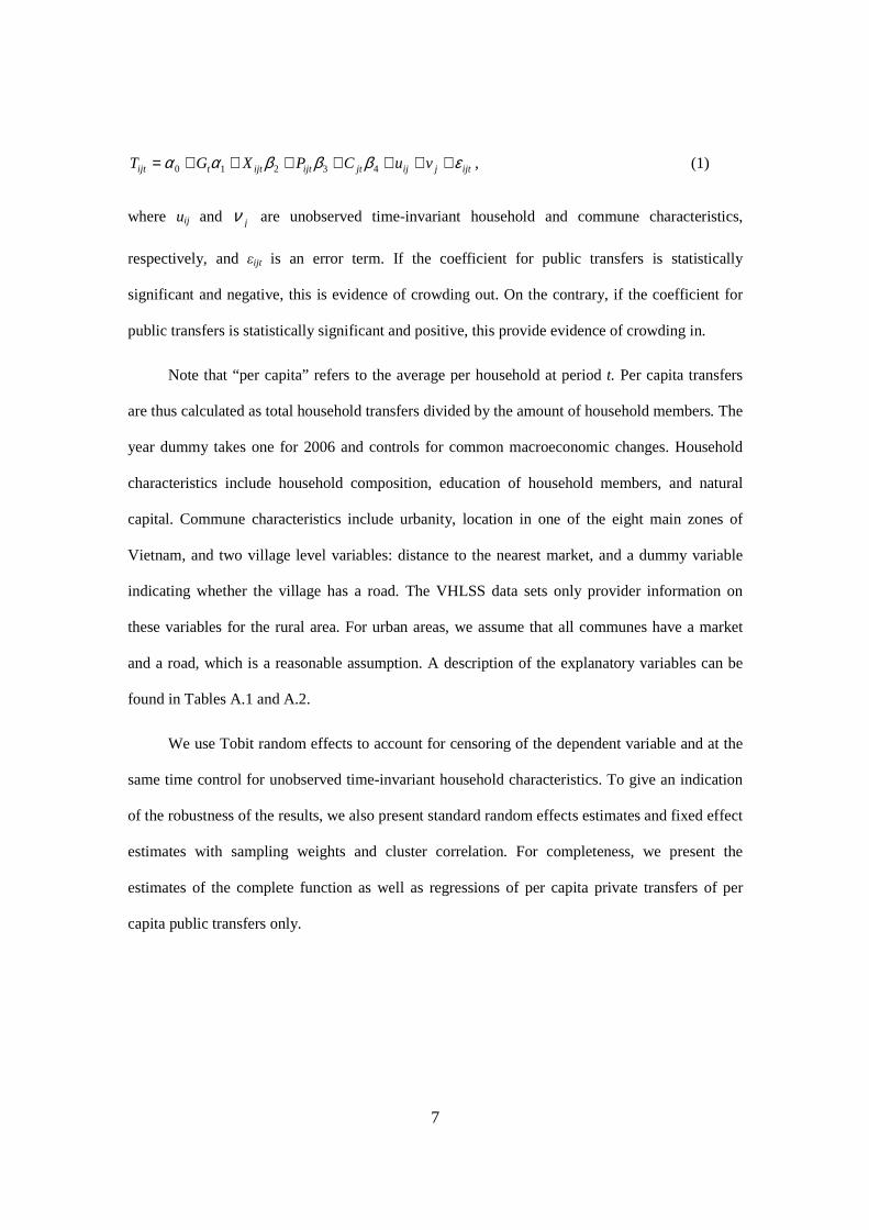
ijtjijjtijtijttijt vuCPXGT εβββαα +++++++= 43210 , (1)

where uij and jν are unobserved time-invariant household and commune characteristics,

respectively, and εijt is an error term. If the coefficient for public transfers is statistically

significant and negative, this is evidence of crowding out. On the contrary, if the coefficient for

public transfers is statistically significant and positive, this provide evidence of crowding in.

Note that “per capita” refers to the average per household at period t. Per capita transfers

are thus calculated as total household transfers divided by the amount of household members. The

year dummy takes one for 2006 and controls for common macroeconomic changes. Household

characteristics include household composition, education of household members, and natural

capital. Commune characteristics include urbanity, location in one of the eight main zones of

Vietnam, and two village level variables: distance to the nearest market, and a dummy variable

indicating whether the village has a road. The VHLSS data sets only provider information on

these variables for the rural area. For urban areas, we assume that all communes have a market

and a road, which is a reasonable assumption. A description of the explanatory variables can be

found in Tables A.1 and A.2.

We use Tobit random effects to account for censoring of the dependent variable and at the

same time control for unobserved time-invariant household characteristics. To give an indication

of the robustness of the results, we also present standard random effects estimates and fixed effect

estimates with sampling weights and cluster correlation. For completeness, we present the

estimates of the complete function as well as regressions of per capita private transfers of per

capita public transfers only.

8

2.2 Impact of transfers on per capita income, per capita expenditure, and labor supply

Transfers increase income, but not necessarily by the amount of money transferred. Increased

availability of non-labor income results in a rise in the shadow price of household labor. If labor

supply is quite flexible, which is the case for self-employed households –an important group in

developing countries like Vietnam– this will result in a decrease in labor supply that partly offsets

the initial income increase. On the other hand, transfers can also provide working capital

investment money for productive activities and therefore increase income by more than the

amount transferred. Similarly, an increase in income does not necessarily result in the same

increase in expenditures. Households may save part of the transfers, and the savings coefficient

may be different from the coefficient for earned income. We therefore estimate not only the

ultimate impact of transfers on expenditures, which –together with the distribution of transfers–

determines their impact on poverty and inequality, but also the impact on income and labor

supply.

We assume a similar specification for estimating the effect of transfers on per capita

income, per capita expenditure and labor supply:

0 1 2 3 4ijt t ijt ijt jt ij j ijtY G X D C uβ β β β β ν ε= + + + + + + + , (2)

where Y is a vector including income per capita, expenditure per capita, and different proxies for

labor supply, D is a vector of per capita public and private transfers and the remainder variables

are identical to equation (1). Van de Walle (2004) uses a similar equation for her estimates of the

impact of public transfers on consumption. Please note that simultaneous inclusion of public and

private transfers in a single equation is only possible when they are independent, that is if public

transfers do not affect private transfers (Heckman et al. 1999). Otherwise, separate regressions

are required for the two types of transfers.

9

We use fixed and a random effects estimators. If the random effects estimator is used0β

is assumed to be the same for all households. In the fixed effects estimator, however, the constant

is allowed to differ per household, i.e. 0 0ijβ β= . The time invariant household and commune

characteristics are then perfectly correlated with the fixed effect and ij ju ν+ will drop out of the

model. The advantage of using panel data estimators is that they correct for time variant

unobserved characteristics, such as diligence and social networks, that affect the choice variables.

These characteristics are likely to be correlated with the independent variables in the regression,

and if so, they will cause estimates to be biased unless fixed effects regression is used. Fixed

effects regression was also used by Van de Walle (2004) in her study on the impact of public

transfers on poverty. In addition, she used 1993 transfers as instruments for 1998 transfers in an

IV regression. However, as she herself admits, the validity of these results depends on the

exogeneity of the instrument. This assumption cannot be tested as there are no other potential

instruments. We are not convinced of the suitability of the instrument and therefore do not follow

the IV approach and focus on the fixed effect regressions.

The marginal impact of transfers is measured by3β . We will also measure the impact of

transfers by calculating the Average Treatment Effect on the Treated (ATT) (Heckman, et al.,

1999), i.e. the impact of transfers on the recipients (with D>0):

( 0)( 0) ( 0)t ijt ijt ijt D ijtATT E Y D E Y D== > − > , (3)

Where )0( )0( >= ijtDijt DYE is the expected value of the outcome variable of the transfers

recipients, i.e. income per capita, expenditure per capita, or work efforts, had they not received

transfers. This is not observed and has to be estimated.

Using equation (2), we get:

( ) ( )( )( ) ( ) 3421043210

0 00

ββββββββββ ijtjtijttjtijtijtt

ijtDijtijtijtt

DCXGCDXG

DYEDYEATT

=+++−++++

=>−>= =., (4)

10

which implies:

∑−

=tn

iijt

tt D

nTTA

13

ˆ1ˆ β , (5)

where nt is the number of the remittance recipients at time t.

We compliment these point estimates of ATT with standard error estimates generated using

a non-parametric bootstrap technique. This bootstrap is implemented by repeatedly drawing

samples from the original data. Since the VHLSSs sample selection follows stratified random

cluster sampling, communes instead of households are bootstrapped in each stratum (Deaton,

1997). The number of replications is 500.3

2.3 The impact of transfers on poverty and inequality

We calculate poverty by three Foster-Greer-Thorbecke poverty indexes, which are all special

cases of the following formula (Foster, Greer and Thorbecke, 1984):

∑=

−=

q

i

i

z

Yz

nP

1

1α

α , (6)

where Yi is a welfare indicator for person i. When α = 0, you get the headcount index, i.e.

the proportion of people below the poverty line. z is the expenditure poverty line, n is the number

of people in the sample population, q is the number of poor people, and α can be interpreted as a

measure of inequality aversion. For α = 1 and α = 2, the indicator represents the poverty gap,

representing the depth of poverty, and the squared poverty gap, representing the severity of

3 We also tried to bootstrap households instead of communes to examine the robustness to the standard error estimates to bootstrap ways. The results from the different bootstrap methods were very similar.

11

poverty, respectively. We use consumption expenditure per capita as the welfare indicator, since,

as is well known, consumption is a better proxy for well-being than income.

To measure inequality, we use three common indexes: the Gini coefficient, Theil’s L index

of inequality, and Theil’s T index of inequality. All three indexes are computed using average per

capita expenditures Y , population size n and individual per capita expenditures. Higher values

imply a more unequal distribution. The Gini index is specified as follows:

∑∑= =

−−

=n

i

n

jji YY

YnnG

1 1)1(2

1, (7)

and ranges from zero to one.

The Theil L index of inequality ranges from zero to infinity and is calculated as follows:

∑=

=

n

i iY

Y

nLTheil

1

ln1

_ , (8)

The Theil T index runs from zero to ln(n) and equals:

∑=

=n

i

ii

Y

Y

Y

Y

nTTheil

1

ln1

_ (9)

The impact of transfers on the poverty and inequality indices of transfer receivers in period

t is calculated as follows:

),0(),0( )0( =>−>=∆ Dtttt YDIYDII , (10)

where the first term on the right-hand side of (9) is the relevant indicator for transfers receiving

households if these households receive transfers. This term is observed and can be estimated

directly from the sample data. However, the second term on the right-hand side of (10) is the

counterfactual measure, i.e., the indicator for receiving households had they not received the

transfers. This term is not observed directly, and is estimated by using predicted expenditure

estimated by equation (2).

12

We also measure the impact of transfers on total poverty and inequality:

)()( )0( =−=∆ Dtt YIYII , (11)

where I(Yt) is the observed index of the entire population and )( )0( =DtYI is the index of the entire

population had the recipients not received the transfers. The difference between equations (11)

and (10) is that the latter only looks at the effect on transfers recipients, while the former

considers the effect on the entire population. As for ATT, the standard errors of the estimates of

impacts on poverty and inequality are computed using bootstrap techniques.

3 Income transfers, poverty and inequality in Vietnam

3.1 Who are the recipients of transfers?

Vietnam’s social security net includes a large number of programs, including both contribution-

based and non-contributed based transfers. Contribution-based social insurance covers health

benefits, which are outside the scope of this paper, and social security schemes, which have been

compulsory for employees in State organizations, State-owned enterprises, and private enterprises

with ten employees or more since 1995 (Evans et al., 2006). These schemes are mainly paid in

cash and include maternity benefits, severance pay, sickness and occupational injury benefits,

monthly pensions for the retired, and life insurance (Government of Vietnam, 1993a, 1993b,

1995, 1998, 2003 and 2006). The main non-contributory schemes are the National Targeted

Programs (NTPs) and social allowances. The NPTs provide very diverse support to the poor and

are often in kind and difficult to convert to monetary values. In this paper, we therefore focus on

social allowances, which are usually disbursed in cash. These cover support to disadvantaged

13

groups, such as war invalids and heroes, the elderly, children without guardians, disabled people,

and households adversely affected by natural calamities (Government of Vietnam, 1993b, 2003).

Table 1 presents the distribution of public transfers by the poor and non-poor in 2004 and

2006. The coverage of public transfers remained almost unchanged during this period. About 18

percent of all households received public transfers in both years. In 2004 this was no different for

the poor and the non-poor, but in 2006 the percentage of the poor receiving public transfers was

decreased to 13.8 percent. In addition, the non-poor received much higher amounts of transfers

per capita in both years. Since the non-poor moreover account for a large proportion of

population, they received more than 95 percent of all public transfers in both years. Yet, the share

of public transfers in income and expenditure for those poor receiving transfers is substantial:

24.0 and 38.1 percent of expenditures in 2004 and 2006, respectively, and 17.4 and 23.2 percent

of income in 2004 and 2006, respectively.

Table 1 Public transfers by poor and non-poor recipients

2004 2006 Indicators

Poor Non Poor All Poor Non Poor All

18.0 18.3 18.3 13.8 18.8 18.1 % receiving households

[1.1] [0.5] [0.5] [1.2] [0.5] [0.5]

361.2 2044.3 1761.5 617.0 2882.5 2648.9 Per capita public transfers (thousand VND)* [31.3] [70.2] [62.4] [74.7] [96.1] [90.6]

16.8 83.2 100 10.3 89.7 100 Distribution of receiving households [1.0] [1.0] [0.9] [0.9]

4.2 95.8 100 3.1 96.9 100 Distribution of public transfers

[0.4] [0.4] [0.4] [0.4]

24.0 34.3 33.8 38.1 41.7 41.6 % of public transfers in household expenditure [2.0] [1.1] [1.1] [4.4] [1.5] [1.5]

17.4 26.7 26.2 23.2 31.0 30.8 % of public transfers in household income [1.4] [0.9] [0.8] [2.3] [1.0] [1.0]

Number of observations 1769 7419 9188 1427 7762 9189 Note: * in 2004 prices. Standard error in bracket (corrected for sampling weight and cluster correlation). Source: Estimation from VHLSSs 2004 and 2006.

By far most households received domestic private transfers: Between 84.0 and 88.7 percent

for the poor and the non-poor in 2004 and 2006 (Table 2). While the shares of households

receiving private transfers did not differ much between the rich and the poor, the non-poor

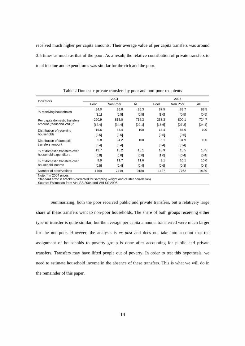
14

received much higher per capita amounts: Their average value of per capita transfers was around

3.5 times as much as that of the poor. As a result, the relative contribution of private transfers to

total income and expenditures was similar for the rich and the poor.

Table 2 Domestic private transfers by poor and non-poor recipients

2004 2006 Indicators

Poor Non Poor All Poor Non Poor All

84.0 86.8 86.3 87.5 88.7 88.5 % receiving households

[1.1] [0.5] [0.5] [1.0] [0.5] [0.5]

220.9 815.0 716.3 238.3 800.1 724.7 Per capita domestic transfers amount (thousand VND)* [12.4] [34.4] [29.1] [16.6] [27.3] [24.1]

16.6 83.4 100 13.4 86.6 100 Distribution of receiving households [0.5] [0.5] [0.5] [0.5]

5.8 94.2 100 5.1 94.9 100 Distribution of domestic transfers amount [0.4] [0.4] [0.4] [0.4]

13.7 15.2 15.1 13.9 13.5 13.5 % of domestic transfers over household expenditure [0.8] [0.6] [0.6] [1.0] [0.4] [0.4]

9.9 11.7 11.6 9.1 10.1 10.0 % of domestic transfers over household income [0.5] [0.4] [0.4] [0.6] [0.3] [0.3]

Number of observations 1769 7419 9188 1427 7762 9189 Note: * in 2004 prices. Standard error in bracket (corrected for sampling weight and cluster correlation). Source: Estimation from VHLSS 2004 and VHLSS 2006.

Summarizing, both the poor received public and private transfers, but a relatively large

share of these transfers went to non-poor households. The share of both groups receiving either

type of transfer is quite similar, but the average per capita amounts transferred were much larger

for the non-poor. However, the analysis is ex post and does not take into account that the

assignment of households to poverty group is done after accounting for public and private

transfers. Transfers may have lifted people out of poverty. In order to test this hypothesis, we

need to estimate household income in the absence of these transfers. This is what we will do in

the remainder of this paper.

15

3.2 Public and private transfers: crowding out or crowding in?

To test for the relation between public and private transfers net of household characteristics, we

ran a regression of private transfers on public transfers and control variables as described above.

While simple regressions of private transfers on public transfers point towards a significantly

positive relation, the significance disappears after the introduction of household fixed effects or

the introduction of household and community controls (Tables 3 and Table A.1 in the Appendix).

Put differently, the positive association between public and private transfers is the consequence of

common association with other characteristics and not of a direct relation: Some households

received both more public and more private transfers than others did, but this is due to other

factors than the crowding in of private transfers by public transfers. For example, households with

more elderly received both more pensions and more transfers from friends and relatives but the

latter sent these not considering the level of public transfers. This result is robust for the

estimation method used.

Table 3 Regression of per capita domestic transfer

Explanatory variables

Random effects

(no sampling weights)

Tobit Random effects


Fixed effects (with

sampling weights and

cluster correlation)

Random effects




Fixed effects (with

sampling weights and


0.122*** 0.122*** -0.006 0.01 0.01 -0.05 Public transfers per capita (thousand VND) [0.013] [0.013] [0.056] [0.014] [0.014] [0.057] Household controls No No No Yes Yes Yes Community controls No No No Yes Yes Yes Dummy variable for 2006

Yes Yes Yes Yes Yes Yes

Constant Yes Yes yes Yes Yes Yes

Observations 8432 8432 8432 8432 8432 8432 Number of households 4216 4216 4216 4216 4216 4216 R-squared 0.01 0.01 0.104 0.07 Standard errors parentheses. * significant at 10%; ** significant at 5%; *** significant at 1%. Source: Estimation from panel data VHLSSs 2004-2006.

16

3.3 Transfers and labor supply

Public and private transfers potentially lower labor supply. To test this relation, we ran

regressions of several indicators of households labor supply on public and private transfers. The

labor variables are the ratio of working members in households, the number of working

household members, total annual working hours per capita, and total working hours per working

household member. The regression results are reported in Tables A.2 and A.3 in the Appendix.

The results are mostly very similar across different estimation methods. As Hausman tests reject

exogeneity of the household effects, we select the fixed effect estimates with survey corrections

to estimate ATT.

The ATT estimates are presented in Table 4 and show clearly that both public and private

transfers decreased work efforts as expected. Receipt of private transfers reduced the ratio of

members working in productive activities to total adult household members by nearly 1

percentage point. The impacts of public transfers on the working to all adult ration was of similar

magnitude, but not statistically significant. Both public and private transfers reduced the working

hours of the recipients. Public transfers on average reduced working hours per capita by 52 hours,

or 5 percent in 2004. The reduction was substantially higher in 2006, when public transfers were

higher: 89 hours, or 8 percent. The effect of domestic private transfers was quite small: The

receipt of private transfers reduced the working hours per capita by only 1 percent in both years.

Not only were private transfers much lower than public transfers, their coefficient in the labor

hours equations was also lower indicating that per VND transferred, the decrease in working

hours was lowest for private transfers. Possible reasons could be that private transfers are better

targeted to those who really need them or that people are afraid that their relatives or friends will

not send money again if they notice that the recipients start working less hours.

17

Table 4 Impact of public and private transfers on annual working hours (ATT)

2004 2006

Y1 Y0 ATT

(Y1 – Y0) Y1 Y0

ATT (Y1 – Y0)

Impact of public transfers on:

69.6*** 70.3*** -0.8 66.5*** 67.8*** -1.3 Members engaged in productive activities/total household members older than 14 (%) [0.7] [1.0] [0.8] [0.8] [1.5] [1.3]

1688.7*** 1766.5*** -77.8*** 1732.9*** 1863.2*** -130.3*** Annual working hours per household member engaged in productive activities [19.3] [27.1] [18.8] [23.2] [38.4] [31.7]

948.3*** 999.8*** -51.5*** 961.4*** 1050.0*** -88.6*** Annual working hours per capita

[12.3] [17.9] [13.7] [15.6] [28.0] [23.7]

Impact of private transfers on:

76.6*** 77.3*** -0.7** 75.1*** 75.9*** -0.8*** Members engaged in productive activities/total household members older than 14 (%) [0.3] [0.4] [0.2] [0.3] [0.4] [0.2]

1776.1*** 1784.7*** -8.6** 1822.5*** 1832.6*** -10.1** Annual working hours per household member engaged in productive activities [10.7] [11.3] [3.4] [10.2] [11.0] [4.0]

1001.9*** 1013.5*** -11.5*** 1040.6*** 1054.0*** -13.4*** Annual working hours per capita

[6.6] [7.6] [3.6] [7.1] [8.1] [4.2] Note: Members engaged in productive activities are those who are above 14 year olds and working for money and working hours are those hours spent in productive activities. * significant at 10%; ** significant at 5%; *** significant at 1% Figures in brackets are standard errors. Standard errors are corrected for sampling weights and estimated using bootstrap (non-parametric) with 500 replications. Source: Estimation from VHLSSs 2004 and 2006

3.4. The effect of transfers on household income and expenditure

Tables A.4 and A.5 in the Appendix present the regressions of income and expenditure per capita

on public and private transfers per capita and other control explanatory variables. As indicated

before, we present both random effects and fixed effects estimates, without and with sampling

weights and cluster correlation. The results as quite robust with respect to estimation method and

inclusion or non-inclusion of control variables. Since the Hausman tests strongly favor the fixed

effects estimates, we focus the discussion on the survey-corrected fixed-effect estimates.

The estimates of marginal effect of public and private transfers on income are 0.75 and

0.72, respectively and not significantly different (Table A.4 in Appendix). This means that an

extra VND transferred per capita lead to an increase of just over 0.7 VND in per capita income,

irrespective of the source of the transfer. The estimates are statistically significantly smaller than

18

one, indicating that income increased by less than the money amount transferred. These findings

are consistent with the findings that transfers decrease work effort ansd do not confirm the

existence of multiplier effects.

As expected, the impact of public and private transfers on expenditures was lower than the

impact on income (Table A.5 in Appendix). An increase of 1 VND in per capita public and

private transfers resulted in an increase of 0.12 and 0.41 VND in per capita expenditure. This

suggests that households use public and private transfers for not only consumption but also for

savings and investment. These results are of the same order of magnitude as the findings of Van

de Walle (2004) who conclude that the propensity to consume out of public transfers (not

including pensions) was 0.37 for Vietnam during the 1990s.

To see the total increase in per capita income and expenditure caused by transfers, we

estimated ATT. Since ATT depends on the size of transfers, it may have differed between years

and sources, and Table 5 presents the ATT estimates for public and private transfers for both

years separately. It shows that public transfers increased per capita income of the recipient by

around 20 and 24 percent in 2004 and 2006, respectively. The effect of public transfers on per

capita expenditure was much lower. Public transfers increased per capita expenditures of the

recipient households only by 3 and 4 percent for the years 2004 and 2006, respectively. Again,

this finding suggests that most public transfers were saved.

Private transfers had a much lower effect on per capita income than public transfers – a 7

and 6 percent increase in 2004 and 2006, respectively– simply because private transfers were

much smaller on average. The effect of both transfers on expenditures was, however, comparable:

private transfers increased recipients per capita expenditure by around 5, public transfers by 3-4

percent. Hence, whereas most public transfers were saved, a relatively large share of private

transfers was used for current consumption. This suggests that people sent more transfers to

relatives and friends who had higher need for consumption, as theories of altruism and insurance

imply.

19

Table 5 Impact of transfers measured by ATT

2004 2006

Y1 Y0 ATT

(Y1 – Y0) Y1 Y0

ATT (Y1 – Y0)

Impact of public transfers on: Income per capita 6279.3*** 5238.0*** 1041.3*** 7962.2*** 6416.5*** 1545.7*** [167.4] [194.3] [120.8] [192.1] [247.9] [183.4] Expenditure per capita 4860.6*** 4699.3*** 161.3** 5938.3*** 5698.9*** 239.4** [117.1] [136.9] [76.8] [140.7] [174.9] [102.4]

880.1*** 1306.3*** Difference in ATT between income and expenditure [109.5] [167.6] Impact of private transfers on:

Income per capita 5801.7*** 5412.6*** 389.1*** 6809.5*** 6420.6*** 388.9***

[89.1] [88.4] [32.3] [99.3] [100.9] [31.9]

Expenditure per capita 4455.1*** 4229.1*** 226.0*** 5034.8*** 4806.4*** 228.4***

[64.9] [71.9] [35.9] [70.5] [76.7] [38.1]

163.1*** 160.5*** Difference in ATT between income and expenditure [37.8] [37.7] * significant at 10%; ** significant at 5%; *** significant at 1% Figures in brackets are standard errors. Standard errors are corrected for sampling weights and estimated using bootstrap (non-parametric) with 500 replications. Source: Estimation from VHLSSs 2004 and 2006

3.5. Impact on poverty and inequality

Since transfers had a significant impact on per capita expenditure, they are expected to have

affected poverty and inequality. Public transfers indeed reduced the head count of poverty of

recipients by around 2.2 and 1.3 percentage points in 2004 and 2006, respectively, although the

effect was not statistically significant for the latter year (Table 6). While the average transfer

amounts were higher in 2006, their effect on poverty was higher in 2004, because in this year

there were more poor and a larger share of the poor received public transfers. The effect of public

transfers on the overall head count was negligible, as was their impact on the other poverty

indexes. This indicates that not much has changed since the 1990s, for which Van de Walle

(2004) obtained a similar result.

20

Table 6 Impact of transfers on poverty

2004 2006

With public transfers

Without public

transfers

Impact With public transfers

Without public

transfers

Impact

Public transfers

Transfer recipients

Head count 0.1991*** 0.2207*** -0.0216** 0.1353*** 0.1483*** -0.0130 [0.0129] [0.0163] [0.0108] [0.0122] [0.0148] [0.0092] Poverty gap 0.0565*** 0.0608*** -0.0044* 0.0388*** 0.0429*** -0.0041 [0.0050] [0.0058] [0.0026] [0.0055] [0.0060] [0.0025] Severity 0.0235*** 0.0251*** -0.0015 0.0160*** 0.0178*** -0.0018 [0.0028] [0.0031] [0.0010] [0.0031] [0.0033] [0.0012] All Head count 0.1949*** 0.1987*** -0.0038** 0.1597*** 0.1620*** -0.0023 [0.0053] [0.0056] [0.0019] [0.0051] [0.0052] [0.0016] Poverty gap 0.0472*** 0.0480*** -0.0008 0.0383*** 0.0390*** -0.0007 [0.0017] [0.0018] [0.0005] [0.0017] [0.0018] [0.0004] Severity 0.0170*** 0.0173*** -0.0003 0.0137*** 0.0140*** -0.0003 [0.0009] [0.0009] [0.0002] [0.0009] [0.0009] [0.0002] Private transfers

Transfer recipients

Head count 0.1884*** 0.2159*** -0.0275*** 0.1574*** 0.1780*** -0.0206***

[0.0060] [0.0077] [0.0050] [0.0062] [0.0078] [0.0047]

Poverty gap 0.0446*** 0.0569*** -0.0123*** 0.0366*** 0.0457*** -0.0092***

[0.0019] [0.0037] [0.0031] [0.0019] [0.0031] [0.0024]

Severity 0.0157*** 0.0338*** -0.0181 0.0128*** 0.0205*** -0.0077**

[0.0009] [0.0125] [0.0124] [0.0009] [0.0038] [0.0036]

All

Head count 0.1953*** 0.2189*** -0.0236*** 0.1601*** 0.1782*** -0.0182***

[0.0058] [0.0071] [0.0043] [0.0059] [0.0074] [0.0041]

Poverty gap 0.0473*** 0.0579*** -0.0106*** 0.0384*** 0.0464*** -0.0081***

[0.0019] [0.0033] [0.0027] [0.0019] [0.0030] [0.0021]

Severity 0.0170*** 0.0325*** -0.0155 0.0137*** 0.0205*** -0.0068**

[0.0009] [0.0107] [0.0106] [0.0009] [0.0034] [0.0032] * significant at 10%; ** significant at 5%; *** significant at 1% Figures in brackets are standard errors. Standard errors are corrected for sampling weights and estimated using bootstrap (non-parametric) with 500 replications. Source: Estimation from VHLSSs 2004 and 2006

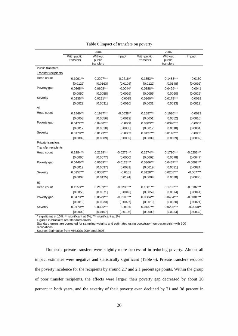
Domestic private transfers were slightly more successful in reducing poverty. Almost all

impact estimates were negative and statistically significant (Table 6). Private transfers reduced

the poverty incidence for the recipients by around 2.7 and 2.1 percentage points. Within the group

of poor transfer recipients, the effects were larger: their poverty gap decreased by about 20

percent in both years, and the severity of their poverty even declined by 71 and 38 percent in

21

2004 and 2006, respectively. As more than 80 percent of the poor received domestic private

transfers, their effects on total poverty were only slightly smaller than their effects on poverty of

recipients alone.

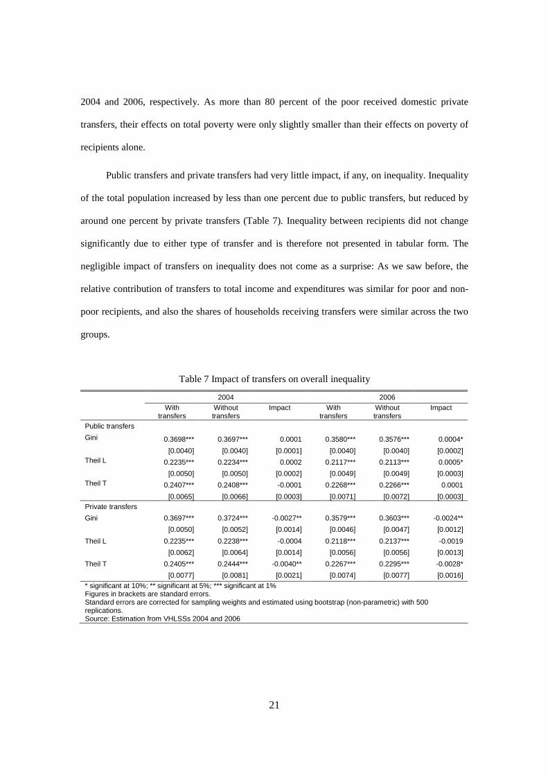
Public transfers and private transfers had very little impact, if any, on inequality. Inequality

of the total population increased by less than one percent due to public transfers, but reduced by

around one percent by private transfers (Table 7). Inequality between recipients did not change

significantly due to either type of transfer and is therefore not presented in tabular form. The

negligible impact of transfers on inequality does not come as a surprise: As we saw before, the

relative contribution of transfers to total income and expenditures was similar for poor and non-

poor recipients, and also the shares of households receiving transfers were similar across the two

groups.

Table 7 Impact of transfers on overall inequality

2004 2006

With transfers

Without transfers

Impact With transfers

Without transfers

Impact

Public transfers Gini 0.3698*** 0.3697*** 0.0001 0.3580*** 0.3576*** 0.0004* [0.0040] [0.0040] [0.0001] [0.0040] [0.0040] [0.0002] Theil L 0.2235*** 0.2234*** 0.0002 0.2117*** 0.2113*** 0.0005* [0.0050] [0.0050] [0.0002] [0.0049] [0.0049] [0.0003] Theil T 0.2407*** 0.2408*** -0.0001 0.2268*** 0.2266*** 0.0001 [0.0065] [0.0066] [0.0003] [0.0071] [0.0072] [0.0003] Private transfers

Gini 0.3697*** 0.3724*** -0.0027** 0.3579*** 0.3603*** -0.0024**

[0.0050] [0.0052] [0.0014] [0.0046] [0.0047] [0.0012]

Theil L 0.2235*** 0.2238*** -0.0004 0.2118*** 0.2137*** -0.0019

[0.0062] [0.0064] [0.0014] [0.0056] [0.0056] [0.0013]

Theil T 0.2405*** 0.2444*** -0.0040** 0.2267*** 0.2295*** -0.0028*

[0.0077] [0.0081] [0.0021] [0.0074] [0.0077] [0.0016] * significant at 10%; ** significant at 5%; *** significant at 1% Figures in brackets are standard errors. Standard errors are corrected for sampling weights and estimated using bootstrap (non-parametric) with 500 replications. Source: Estimation from VHLSSs 2004 and 2006

22

4 Conclusion

In this study, we investigate how well public transfers and domestic private transfers reached the

poor in Vietnam and to which extent these transfers affected poverty and inequality in the mid-

2000s. We also show some of the other underlying mechanisms. We estimate the effect of the

transfers on both per capita income and expenditure. Neither is straightforward. Cash transfers do

not necessarily result in an increase in income with the same value as the transfer. On the one

hand, cash transfers may have positive multiplier effects when (part of) the money is used

productively. On the other hand, public transfers may crowd out private transfers and lead to a

reduction of work effort. We therefore also estimate the effect of public transfers on domestic

private transfers and the effect of both types of transfers on work effort. At the same time, the

propensity to consume is not necessarily the same for transfers and earned income, as they may

accrue to different persons with different preferences, and money may not be perfectly pooled.

Last but not least, estimating the effect of transfers on income and expenditures will give biased

estimates unless the endogeneity of transfer allocation is accounted for. We therefore use fixed-

effects regression to account for time-invariant unobserved variables that are correlated with the

independent variables.

Vietnam’s extensive social security system is claimed to have played a key role in the

extraordinary poverty decline over the past decades. This claim is, however, not substantiated by

empirical evidence. Like Van de Walle (2004) has shown for the 1990s, we find that the impact

of public transfers on poverty was negligible due to low coverage of poor and relatively low

amounts transferred to the poor, but not due to crowding out of private transfers: Contrary to

studies for other countries, our estimates suggest that public transfers did not affect the level of

private transfers. Still, the effect of transfers received on expenditures was small: transfer

recipients decreased labor supply and in addition used only a limited amount of the extra income

for current consumption.

23

Domestic private transfers were somewhat more successful in reducing poverty – a

decrease of about two percentage points of the head count and quite substantial decreases in the

depth and severity of poverty– because a large proportion of the poor received private transfers

and a relatively high share of private transfers was used for current consumption.

Our results imply that simply increasing the government budget for transfers will not be

very effective in decreasing poverty. A significant share of transfers will leak to the non-poor,

even though social subsidies alone are targeting slightly better than the overall transfers we

present in the paper. Moreover, as indicated above, the impact of public transfers received on

expenditures is low. The much larger effect of private transfers, however, indicates that better

targeting could also improve the link between transfers and expenditures.

Better targeting is however complicated and possibly costly. Decentralization, as

suggested by Van de Walle (2004), may not be an easy solution. Public microfinance is allocated

through commune authorities to supposedly poor households. Still, two thirds of the money lent

ends up with the non-poor (Nguyen et al, 2008). Our results suggests that facilitation of money

transfers between relatives and friends could be a more efficient method of decreasing poverty.

Despite the fact that most public and private transfer went to non-poor households,

inequality was only marginally affected. The group of non-poor is much larger than the group of

poor households, and even though the average transfer received is much higher for non-poor

recipients, the relative contribution of transfers to total income and expenditures was similar for

the poor and the non-poor recipients. Also, the shares of households receiving transfers

were similar across the two groups for both public and private transfers.

Finally, we must keep in mind that our poverty and inequality estimates do not cover all

effects of transfers on welfare. A substantial share of especially public transfers seems to be saved

or invested and may thus lead to future improvements in well-being, which was outside the scope

of this study. Also, transfers resulted in a decrease in work effort and thus an increase in leisure,

24

which – like consumptive expenditures – adds to current welfare, but is not accounted for in our

poverty calculations.

References

Alderman, H. and T. Haque (2006), “Countercyclical Safety Nets for the Poor and Vulnerable”,

Food Policy 31(4), 372-383.

Barrientos, A. and J. DeJong (2006), “Reducing Child Poverty with Cash Transfers: A Sure

Thing?”, Development Policy Review 24(5): 537–552

Barro, R. J. (1974), “Are Government Bonds Net Wealth?”, Journal of Political Economy 82:

1095–1117.

Becker, G. (1974), “A Theory of Social Interactions”, Journal of Political Economy 82: 1063–

1093.

Bernheim, D., A. Shleifer, and L. Summers (1985), “The Strategic Bequest Motive”, Journal of

Political Economy 93: 1945–1076.

Carter, M. R. and C. B. Barrett (2006), “The Economics of Poverty Traps and Persistent Poverty:

An Asset-Based Approach”, Journal of Development Studies 42(2): 178-199.

Castles F.G., and D. Mitchell (1993), “Worlds of Welfare and Families of Nations”, In Families

of Nations: Patterns of Public Policy in Western Democracies edited by Castles, F.G. Dartmouth:

Dartmouth University Press.

Cox, D. (1987), “Motives for Private Income Transfers”, Journal of Political Economy 95: 508–

546.

25

Cox, D. (1990), “Intergenerational Transfers and Liquidity Constraints”, Quarterly Journal of

Economics 105: 187–217.

De Brauw, A. and T. Harigaya (2007), “Seasonal Migration and Improving Living Standards in

Vietnam”, American Journal of Agricultural Economics 89(2): 430-447.

De la Brière, B., E. Sadoulet, A. de Janvry and S. Lambert (2002), “The Roles of Destination,

Gender, and Household Composition in Explaining Remittances: An Analysis for the Dominican

Sierra”, Journal of Development Economics 68(2): 309-28.

Dercon, S. (2003), “Risk and Poverty: A Selective Review of the Issue”, Working paper Oxford:

University of Oxford.

Dercon, S. and P. Krishnan (2000), “Vulnerability, Seasonality and Poverty in Ethiopia”, Journal

of Development Studies 36(6): 25-53.

Evans, M., I. Gough, S.N. Harkness, A. McKay, H. D. Thanh and N. D. L. Thu (2006), “How

Progressive is Social Security in Viet Nam?”, Report of UNDP Vietnam, Nov 2006.

Farrington, J. and R. Slater (2006), “Introduction: Cash Transfers: Panacea for Poverty Reduction

or Money Down the Drain?”, Development Policy Review, 2006, 24(5): 499–511

Foster, J., J. Greer, E. Thorbecke (1984), “A Class of Decomposable Poverty Measures”,

Econometrica 52: 761-765.

Friedman, M. and R. Friedman (1979), Free to Choose, Harcourt Brace Jovanovich.

Government of Vietnam (1993a), “ The Government Decree 43-CP dated June 22nd, 1993 on

Temporary Regulations of Social Insurance Schemes”.

Government of Vietnam (1993b), “The Government Decree Number 27/1993/ND-CP on

Regulation of Pension and Social Allowances dated 23/5/1993”.

Government of Vietnam (1995), “The Government Decree N012/CP dated January 26th, 1995 on

Regulations of New Social Insurance Scheme”.

26

Government of Vietnam (1998), “The Government Decree Number 93/1998/ND-CP on

Amending and Supplementing Provisions of Social Insurance Regulations, Issued in Attachment

to the Government Decree No. 121/CP dated 26/1/1995”.


Adjustment of Pensions, Social Allowances, and Renewal of Pension Management dated

15/1/2003”.


Guidelines of Law on Social Insurance and Compulsory Social Insurance dated 22/11/2006”.

Heckman, J., R. Lalonde and J. Smith (1999), "The Economics and Econometrics of Active

Labor Market Programs", Handbook of Labor Economics 3, Ashenfelter, A. and D. Card, eds.,

Amsterdam: Elsevier Science.

Hoddinott, J. (1994). A model of migration and remittances applied to Western Kenya, Oxford

Economic Papers 46: 450-75.

Howe, N. and P. Longman (1992), "The Next New Deal", Atlantic Monthly, April: 88- 99.

Jalan, J. and M. Ravallion (2000), “Is Transient Poverty Different? Evidence for Rural China”,

Journal of Development Studies 36(6): 82-99.

Jensen, R. T. (2003), “Do Private Transfers Displace’ the Benefits of Public Transfers? Evidence

from South Africa”, Journal of Public Economics 88: 89–112.

Lloyd-Sherlock, P. (2006), “Simple Transfers, Complex Outcomes: The Impacts of Pensions on

Poor Households in Brazil”, Development and Change 37(5): 969-995.

Lucas, R. and O. Stark (1985), “Motivations to Remit: Evidence from Botswana” Journal of

Political Economy, 93(5): 901–18.

Maitra, P. and R. Ray (2003), “The Effect of Transfers on Household Expenditure Patterns and

Poverty in South Africa”, Journal of Development Economics 71(1): 23-49

27

Nguyen, V. C., M. M. Van den Berg and D. Bigman (2007) The impact of Micro-credit

on Poverty and Inequality: The Case of the Vietnam Bank for Social Policies. Paper

presented at: Microfinance: What Do We Know? 7-8 December 2007, Groningen, The

Netherlands.

Ravallion, M. (1988), “Expected Poverty under Risk-Induced Welfare Variability”, Economic

Journal 98(393): 1171-1182.

Rosenzweig, M.R. (1988), “Risk, Implicit Contracts and The Family in Rural Areas of Low

Income Countries”, Economic Journal 393: 1148-70.

Sadoulet, E., A. De Janvry, and B. Davis (2001), “Cash Transfer Programs with Income

Multipliers: PROCAMPO in Mexico”, World Development 29(6): 1043-1056.

Sahn, E. D. and H. Alderman (1996) “The Effect of Food Subsidies on Labor Supply in Sri

Lanka”, Economic Development and Cultural Change 45(1): 125-145.

Stark, O. (1995), Altruism and Beyond, Oxford and Cambridge: Basil Blackwell.

Stark, O. and D. Bloom, 1985, “The New Economics of Labor Migration,” American Economic

Review, 75: 173–178.

Stark, O. and D. Levhari (1982), “On Migration and Risk in LDCs”, Economic Development and

Cultural Change 31: 191-6.

Van de Walle, D. (2004), “Testing Vietnam’s Public Safety Net”, Journal of Comparative

Economics 32(4): 661-679.

28

Appendix Regression results

Table A.1 Regression of per capita domestic transfers


Random effects

(no sampling weight)



Fixed effects (with

sampling weight and


Random effects




Fixed effects (with

sampling weight and


0.122*** 0.122*** -0.006 0.01 0.01 -0.05 Public transfers per capita (thousand VND) [0.013] [0.013] [0.056] [0.014] [0.014] [0.057]

-175.680* -176.004* 175.427 Ratio of members younger than 16 to total household members [90.769] [90.521] [241.609]

587.087*** 587.388*** 347.955 Ratio of members who older than 60 to total household members [78.472] [78.241] [357.933]

Household size -452.273*** -451.976*** -728.132*** [33.611] [33.537] [111.687] Household size squared 29.519*** 29.505*** 43.240*** [2.999] [2.992] [8.919]

632.373*** 632.533*** 265.515 Ratio of household member with technical degree [109.205] [108.979] [236.676]

358.895** 361.075** -1156.429* Ratio of household member with post secondary [152.531] [152.304] [615.681]

-0.023** -0.022** -0.054** Area of annual crop land per capita (m2) [0.010] [0.010] [0.022]

-0.003 -0.003 -0.036* Area of perennial crop land per capita (m2) [0.013] [0.013] [0.021]

0.002 0.002 -0.006 Forestry land per capita (m2)

[0.007] [0.007] [0.005] -0.038 -0.038 -0.047 Area of aquaculture water

surface per capita (m2) [0.027] [0.027] [0.031] Road to village (yes = 1) 30.069 29.815 114.498 [49.419] [49.346] [76.938]

0.326 0.319 0.725 Distance to nearest daily market (km) [2.857] [2.853] [2.519] Red River Delta Base-Omitted North East -184.348*** -184.409*** [60.207] [59.995] North West -157.031* -157.042* [93.983] [93.658] North Central Coast -111.363* -111.382* [63.447] [63.220] South Central Coast -165.311** -165.301** [68.170] [67.926] Central Highlands -138.650* -138.705* [83.616] [83.324] North East South 156.528** 156.510** [64.277] [64.049] Mekong River Delta 96.697* 96.663* [56.643] [56.447] Living in urban areas -118.389* -118.010* [60.634] [60.492] Dummy variable for 2006 60.852** 60.839** 97.859*** 39.405 39.399 69.686** [27.533] [27.552] [32.321] [27.273] [27.295] [33.886] Constant 495.59*** 495.56*** 562.86*** 1904.46*** 1903.31*** 2713.51***

29


Random effects




Fixed effects (with

sampling weight and


Random effects




Fixed effects (with

sampling weight and


[23.248] [23.239] [27.718] [105.308] [105.085] [329.116]

Observations 8432 8432 8432 8432 8432 8432 Number of households 4216 4216 4216 4216 4216 4216 R-squared 0.01 0.01 0.104 0.07 Standard errors in brackets. * significant at 10%; ** significant at 5%; *** significant at 1%. Source: Estimation from panel data VHLSSs 2004-2006.

Table A.2 Regressions of the ratio and number of household working members

The ratio of working members in households The number of working members in households


Random effects


Fixed effects (no sampling

weight)

Fixed effects with

sampling weight and

cluster correlation

Fixed effects Poisson


Random effects


Fixed effects with

sampling weight and

cluster correlation

-0.000016*** -0.000004 -0.000005 -0.000047*** -0.000018 -0.000018 Public transfers per capita (thousand VND) [0.000002] [0.000004] [0.000005] [0.000007] [0.000012] [0.000013]

-0.000015*** -0.000009*** -0.000011*** -0.000029*** -0.000013** -0.000019** Domestic transfers per capita (thousand VND) [0.000002] [0.000002] [0.000003] [0.000005] [0.000007] [0.000008]

0.382969*** 0.535524*** 0.557634*** -2.375293*** -1.719399*** -1.591811*** Ratio of members younger than 16 to total household members [0.014132] [0.027685] [0.032667] [0.047787] [0.093710] [0.110253]

-0.232018*** -0.253573*** -0.260653*** -0.666633*** -0.562667*** -0.555223*** Ratio of members who older than 60 to total household members [0.012449] [0.030160] [0.047527] [0.042089] [0.102087] [0.108782]

Household size -0.087057*** -0.103748*** -0.111368*** 0.522134*** 0.521758*** 0.458883*** [0.005229] [0.009347] [0.012851] [0.017684] [0.031637] [0.064394] Household size squared 0.005259*** 0.006395*** 0.006913*** -0.000162 0.001809 0.007073 [0.000463] [0.000807] [0.001099] [0.001566] [0.002732] [0.006610]

0.076530*** 0.099930*** 0.105840*** 0.228553*** 0.341362*** 0.358640*** Ratio of household member with technical degree [0.016207] [0.023968] [0.028146] [0.054835] [0.081130] [0.092228]

0.049526** 0.247522*** 0.239809*** 0.200565** 0.833628*** 0.797131*** Ratio of household member with post secondary [0.023577] [0.044103] [0.055843] [0.079732] [0.149283] [0.175584]

0.000007*** 0.000004 0.000005 0.000010* -0.000001 0.000002 Area of annual crop land per capita (m2) [0.000002] [0.000003] [0.000003] [0.000005] [0.000009] [0.000010]

0.000003 0.000002 0.000004* 0.000004 0.000002 0.000008 Area of perennial crop land per capita (m2) [0.000002] [0.000003] [0.000003] [0.000007] [0.000010] [0.000008] Forestry land per capita (m2) 0.000001 0.000001 0.000001 0.000007* 0.000007 0.000007 [0.000001] [0.000002] [0.000001] [0.000004] [0.000005] [0.000007]

0.000004 0.000007 0.000004 0.000009 0.000022 0.000012 Area of aquaculture water surface per capita (m2) [0.000004] [0.000006] [0.000008] [0.000013] [0.000019] [0.000026] Road to village (yes = 1) 0.000412 0.002517 0.002502 0.003726 -0.001028 0.01421 [0.007113] [0.009355] [0.010194] [0.024074] [0.031666] [0.034545]

0.000132 -0.001125** -0.001323*** -0.00175 -0.005325*** -0.006523*** Distance to nearest daily market (km) [0.000407] [0.000520] [0.000424] [0.001378] [0.001760] [0.001900] Red River Delta Base - Omitted North East 0.030974*** 0.125874*** [0.009907] [0.033478] North West 0.029552* 0.087585* [0.015397] [0.052031]

30

The ratio of working members in households The number of working members in households


Random effects



weight)

Fixed effects with

sampling weight and

cluster correlation



Random effects


Fixed effects with

sampling weight and

cluster correlation

North Central Coast -0.023184** -0.123077*** [0.010475] [0.035395] South Central Coast -0.011081 -0.05888 [0.011256] [0.038034] Central Highlands 0.009184 -0.063221 [0.013717] [0.046356] North East South -0.037660*** -0.146068*** [0.010590] [0.035785] Mekong River Delta -0.016261* -0.019884 [0.009279] [0.031357] Urban -0.078730*** -0.256460*** [0.009370] [0.031686] Time change (dummy 2006) -0.014336*** -0.013058*** -0.010233*** -0.039823*** -0.026673** -0.01988 [0.003451] [0.003557] [0.003933] [0.011692] [0.012039] [0.013132] Constant 1.033248*** 1.012347*** 1.022314*** 0.966159*** 0.642359*** 0.743344*** [0.016954] [0.027480] [0.036347] [0.057338] [0.093016] [0.151506]

Observations 8432 8432 8432 7998 8432 8432 Number of i 4216 4216 4216 3999 4216 4216 R-squared 0.24 0.13 0.17 0.62 0.40 0.39

Test H0: Coefficients of per capita public and private transfers are equal: F-test 0.12 1.21 1.17 3.98 0.13 0.01 P-value 0.73 0.27 0.28 0.05 0.72 0.92 Note: Working people are those who are older than 14 and was working during the past 12 months. Standard errors in brackets. * significant at 10%; ** significant at 5%; *** significant at 1%. Source: Estimation from panel data VHLSSs 2004-2006.

Table A.3 Regressions of annual working hours

Annual working hours per capita Annual working hours per working members


Random effects



weight)

Fixed effects with

sampling weight and

cluster correlation



Random effects


Fixed effects with

sampling weight and

cluster correlation

-0.0522*** -0.0383*** -0.0373*** -0.0621*** -0.0592*** -0.0578*** Public transfers per capita (thousand VND) [0.0046] [0.0079] [0.0092] [0.0065] [0.0116] [0.0131]

-0.0287*** -0.0146*** -0.0212*** -0.0286*** -0.0117* -0.0159** Domestic transfers per capita (thousand VND) [0.0034] [0.0042] [0.0066] [0.0048] [0.0062] [0.0067]

-861.0810*** -642.9849*** -622.3706*** 109.2682*** 20.892 -9.0937 Ratio of members younger than 16 to total household members [30.5052] [60.6844] [62.0347] [42.2936] [88.7716] [92.6954]

-622.6396*** -594.5159*** -622.3082*** -638.8280*** -560.9002*** -632.9537*** Ratio of members who older than 60 to total household members [26.8412] [66.1097] [117.3814] [37.0456] [96.7079] [149.1159]

Household size -84.5288*** -92.4649*** -105.5759*** 111.9003*** 109.9197*** 120.5789*** [11.2961] [20.4873] [28.0074] [15.7102] [29.9697] [33.6507] Household size squared 4.3051*** 4.9081*** 6.1223** -9.7184*** -8.8168*** -9.3359*** [1.0004] [1.7691] [2.3851] [1.3924] [2.5880] [2.7553]

204.6983*** 207.6632*** 219.1755*** 189.4508*** 110.9633 101.5769 Ratio of household member with technical degree [35.1042] [52.5378] [59.8074] [49.3263] [76.8545] [75.2016] Ratio of household member 254.9810*** 606.3869*** 567.0869*** 253.9589*** 365.4885*** 279.2423*

31

Annual working hours per capita Annual working hours per working members


Random effects



weight)

Fixed effects with

sampling weight and

cluster correlation



Random effects


Fixed effects with

sampling weight and

cluster correlation

with post secondary [50.9199] [96.6728] [119.5864] [70.7382] [141.4170] [164.9665] -0.0047 -0.0023 -0.0015 -0.0160*** -0.0003 0.0011 Area of annual crop land per

capita (m2) [0.0034] [0.0061] [0.0073] [0.0048] [0.0089] [0.0095] -0.0045 0.0029 0.0053 -0.0066 0.0052 0.0072 Area of perennial crop land

per capita (m2) [0.0042] [0.0065] [0.0060] [0.0059] [0.0094] [0.0094] Forestry land per capita (m2) -0.0001 0.0025 0.0044 -0.0052 -0.0021 0.001 [0.0023] [0.0035] [0.0038] [0.0032] [0.0051] [0.0082]

0.0026 0.0246** 0.0195 -0.0002 0.0457*** 0.0386* Area of aquaculture water surface per capita (m2) [0.0086] [0.0121] [0.0190] [0.0122] [0.0177] [0.0202] Road to village (yes = 1) 33.3237** 27.8409 31.555 64.2529*** 57.2822* 57.1035* [15.4357] [20.5064] [21.1830] [21.8505] [29.9976] [31.5280]

-0.9876 -1.255 -1.0599 -1.5618 1.1088 1.7374 Distance to nearest daily market (km) [0.8843] [1.1397] [1.4075] [1.2549] [1.6672] [1.9975] Red River Delta Base - Omitted North East 70.3721*** 46.6676 [21.2961] [29.0598] North West -4.4096 -46.4395 [33.1057] [45.2224] North Central Coast -35.6299 -2.1825 [22.5110] [30.6886] South Central Coast -28.5502 -5.8663 [24.1898] [32.9778] Central Highlands -18.8099 -34.9837 [29.4929] [40.2753] North East South 58.3876** 171.9581*** [22.7620] [31.0493] Mekong River Delta -89.0716*** -145.3682*** [19.9517] [27.2551] Urban 128.9550*** 424.9175*** [20.2261] [28.0585] Time change (dummy 2006) 14.6515* 15.4553** 16.8698* 40.6626*** 33.9214*** 30.2728** [7.5408] [7.7960] [9.4689] [10.9984] [11.4043] [13.9251] Constant 1565.56*** 1528.79*** 1558.68*** 1429.47*** 1497.35*** 1497.67*** [36.6225] [60.2355] [81.8858] [50.9213] [88.1150] [99.4892]

Observations 8432 8432 8432 7998 8432 8432 Number of i 4216 4216 4216 3999 4216 4216 R-squared 0.23 0.19 0.08 0.21 0.03 0.10

Test H0: Coefficients of per capita public and private transfers are equal: F-test 16.8 7.13 2.1 17.29 13.34 9.27 P-value 0.00 0.01 0.15 0.00 0.00 0.00 Note: Working people are those who are older than 14 and was working during the past 12 months. Standard errors in brackets. * significant at 10%; ** significant at 5%; *** significant at 1%. Source: Estimation from panel data VHLSSs 2004-2006.

32

Table A.4 Regressions of per capita income


Random effects



weight)

Fixed effects with sampling

weight and cluster

correlation

Random effects



weight)


weight and cluster

correlation 0.846*** 0.764*** 0.807*** 0.574*** 0.718*** 0.754*** Public transfers per capita

(thousand VND) [0.052] [0.086] [0.085] [0.052] [0.086] [0.086] 0.874*** 0.756*** 0.734*** 0.809*** 0.733*** 0.717*** Domestic transfers per capita

(thousand VND) [0.038] [0.046] [0.052] [0.037] [0.046] [0.053] -1209.630*** 41.244 794.221 Ratio of members younger

than 16 to total household members [340.601] [654.724] [1115.817]

-2897.496*** -1852.319*** -1744.062* Ratio of members who older than 60 to total household members [300.478] [713.258] [1039.516]

Household size -351.140*** -696.568*** -705.331* [125.904] [221.038] [373.200] Household size squared 7.478 35.461* 38.979 [11.145] [19.087] [27.459]

4369.924*** 2070.701*** 2469.826*** Ratio of household member with technical degree [389.054] [566.831] [697.994]

10634.727*** 4308.865*** 4787.906*** Ratio of household member with post secondary [567.907] [1043.004] [1853.079]

0.588*** 0.617*** 0.661*** Area of annual crop land per capita (m2) [0.038] [0.066] [0.144]

0.428*** -0.036 -0.091 Area of perennial crop land per capita (m2) [0.047] [0.070] [0.199]

0.031 0.024 0.027 Forestry land per capita (m2)

[0.026] [0.038] [0.062] 0.664*** 0.359*** 0.345*** Area of aquaculture water

surface per capita (m2) [0.096] [0.130] [0.129] Road to village (yes = 1) 366.511** 404.257* 551.506** 366.511** 404.257* 551.506**

[170.391] [221.243] [226.240] Distance to nearest daily market (km) -31.360*** -9.752 -9.493* Red River Delta Base-Omitted [9.749] [12.296] North East -532.061** North West [239.992] -1816.938*** North Central Coast [372.864] -939.537*** South Central Coast [253.812] -3.238 Central Highlands [272.737] -760.104** North East South [332.220] 1733.176*** Mekong River Delta [256.558] 475.643** Living in urban areas [224.707] 2441.156*** Dummy variable for 2006 1135.392*** 1156.466*** 1089.688*** 1000.029*** 1057.636*** 1003.889*** [81.878] [82.434] [101.077] [81.995] [84.111] [113.807] Constant 4980.469*** 5067.907*** 5366.408*** 5220.098*** 6617.513*** 6546.798*** [92.997] [67.703] [64.992] [408.333] [649.881] [1276.726]

33


Random effects



weight)


weight and cluster

correlation

Random effects



weight)


weight and cluster

correlation Observations 8432 8432 8432 8432 8432 8432 Number of households 4216 4216 4216 4216 4216 4216 R-squared 0.11 0.13 0.11 0.3 0.16 0.17

Test H0: Coefficients of per capita public and private transfers are equal: F-test 0.18 0.01 0.6 13.6 0.03 0.16 P-value 0.67 0.93 0.44 0.00 0.87 0.69 Hausman test χ2 (prob) (H0: Difference in coefficients in fixed and random effects regression not systematic)

84.34(0.000) 72.35(0.000)

Standard errors in brackets. * significant at 10%; ** significant at 5%; *** significant at 1%. Source: Estimation from panel data VHLSSs 2004-2006.

Table A.5 Regression of per capita expenditure


Random effects



weight)


weight and cluster

correlation

Random effects



weight)


weight and cluster

correlation 0.379*** 0.136*** 0.162*** 0.142*** 0.100** 0.117** Public transfers per capita

(thousand VND) [0.028] [0.041] [0.056] [0.026] [0.041] [0.056] 0.569*** 0.452*** 0.447*** 0.516*** 0.421*** 0.412*** Domestic transfers per capita

(thousand VND) [0.019] [0.022] [0.068] [0.018] [0.022] [0.069] -1562.752*** -630.642** -540.747 Ratio of members younger

than 16 to total household members [171.155] [310.855] [333.894]

-1323.541*** -1047.050*** -983.324 Ratio of members who older than 60 to total household members [151.773] [338.646] [646.102]

Household size -359.691*** -705.201*** -824.491*** [63.056] [104.946] [159.557] Household size squared 12.358** 35.173*** 46.497*** [5.577] [9.062] [14.457]

2709.662*** 711.208*** 786.982** Ratio of household member with technical degree [192.811] [269.124] [389.883]

8048.395*** 1987.302*** 1985.190** Ratio of household member with post secondary [284.784] [495.205] [932.498]

0.118*** 0.119*** 0.117*** Area of annual crop land per capita (m2) [0.019] [0.031] [0.024]

0.153*** 0.123*** 0.128*** Area of perennial crop land per capita (m2) [0.023] [0.033] [0.036]

-0.01 -0.026 -0.032*** Forestry land per capita (m2)

[0.013] [0.018] [0.010] 0.153*** 0.034 0.032 Area of aquaculture water

surface per capita (m2) [0.047] [0.062] [0.067] Road to village (yes = 1) 9.82 -33.86 33.494 [83.834] [105.044] [124.570]

-11.984** -2.718 -3.923 Distance to nearest daily market (km) [4.785] [5.838] [3.172] Red River Delta North East -643.976*** [122.826]

34


Random effects



weight)


weight and cluster

correlation

Random effects



weight)


weight and cluster

correlation North West -1126.563*** [190.627] North Central Coast -638.732*** [130.019] South Central Coast -3.249 [139.710] Central Highlands -516.445*** [169.883] North East South 1171.448*** [131.345] Mekong River Delta 112.034 [114.875] Living in urban areas 2153.831*** [113.708] Dummy variable for 2006 526.461*** 570.941*** 550.712*** 441.581*** 505.639*** 483.726*** [39.294] [39.178] [50.505] [39.315] [39.935] [54.171] Constant 3900.198*** 4035.709*** 4272.106*** 4909.112*** 6472.702*** 6900.150*** [51.859] [32.177] [55.191] [204.735] [308.556] [445.349]

Observations 8432 8432 8432 8432 8432 8432 Number of households 4216 4216 4216 4216 4216 4216 R-squared 0.16 0.14 0.15 0.46 0.18 0.16 Test H0: Coefficients of per capita public and private transfers are equal: F-test 29.98 46.68 15.11 141.03 49.68 16.8 P-value 0.00 0.00 0.00 0.00 0.00 0.00 Hausman test χ2 (prob) (H0: Difference in coefficients in fixed and random effects regression not systematic)

132.9(0.000) 269.65(0.000)

Standard errors in brackets. * significant at 10%; ** significant at 5%; *** significant at 1%. Source: Estimation from panel data VHLSSs 2004-2006.

impacts of public and private transfers -nguyen and van den berg

Documents