impeller design using cad techniques and conformal mapping ... · impeller design using cad...

3

Impeller Design Using CAD Techniques and Conformal Mapping Method

Milos Teodor “Politehnica” University of Timisoara,

Romania

1. Introduction

Computerized pump design has become a standard practice in industry, and it is widely used for both new designs as well as for old pumps retrofit. Such a complex design code has been developed over the past decade by the author. However, any design method has to accept a set of hypotheses that neglect in the first design iteration the three-dimensional effects induced by the blade loading, as well as the viscous effects. As a result, an improved design can be achieved only by performing a full 3D flow analysis in the pump impeller, followed by a suitable correction of the blade geometry and/or the meridian geometry. This chapter presents a fully automated procedure for generating the inter-blade channel 3D geometry for centrifugal pump impeller, starting with the geometrical data provided by the quasi-3D code. This is why we developed an original procedure that successfully addresses all geometrical particularities of a centrifugal pump.

2. Domain generation of axial-symmetric flow in impeller area

Fluid movement in the impeller area is axially symmetric. The reference system adequate to

this kind of flow is cylindrical (r,θ,z). Because of geometric axial symmetry of the domain

area we have axial-flow symmetry and cinematic, so the study of spatial movement can be

reduced to the study of plane movements, or in a meridian plane, plane containing the

rotation axis of symmetry, Oz. The resolution must be analytical in order to continue to

analytically generate the mesh network to simulate the flow by Finite Element Method

(FEM). The inlet data are the main dimensions of the preliminary study. First axial and

radial extensions should be set. Axial extension, fig. 1, shall be determined based on

previous studies (Gyulai, 1988) relation:

max 01,1z D= ⋅ (1)

Radial expansion is taken by 25% over D2ex diameter (D2-extended). At the mixed-flow-impellers, impeller diameter output, D2, is in the area of transition from axial to radial movement. Therefore the domain must be extended to at least 2D0. So if D2 < 2D0 then

D2ex=2D0, and if D2≥2D0, then D2ex=D2. From D2ex we calculate D2max with the relationship:

2 max 21,25 exD D= ⋅ (2)

www.intechopen.com

Centrifugal Pumps

34

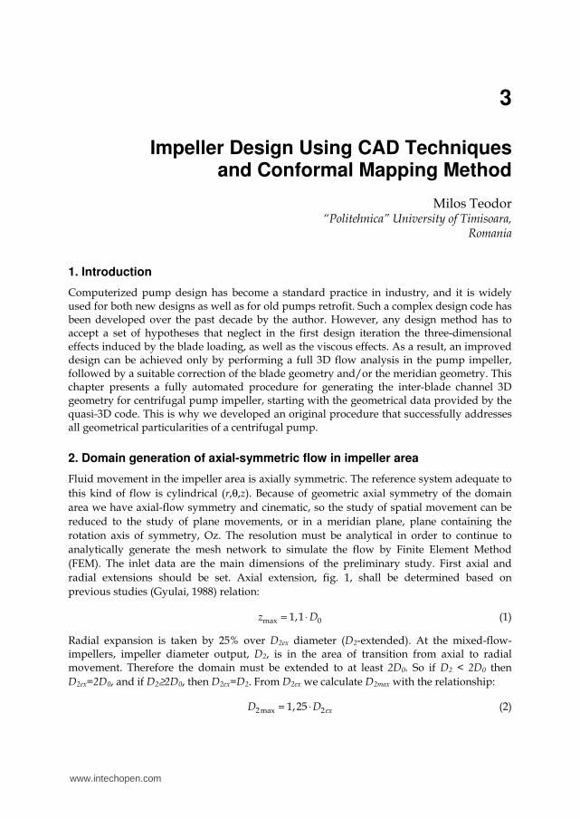
Fig. 1. Geometric construction of half-domain of flow

Zmax and D2max define dimensions of the gauge domain. Next axial area with radial area is connected. Because of technological reasons the shroud connection is made with a straight segment GH and an arc of radius Ri and at the hub only an arc of radius Rc. Input section AB is determined by the input diameter D0 and output section EF of diameter D2max and width b2. First the shroud connection is done by and depending of its position is determined the hub radius Rc and its centre position. The starting point is G at D2G=1,05D2ex. D2G is placed by 5% above D2ex because if D2ex = D2 then in the vicinity of G appear some inflections in meridian speeds variation which will distort the speed triangles of output. From G goes

straight (Di) tilted from the vertical at angle δ = 2° ... 8°. Angle δ is chosen in an initial approximation for nq-low around 2°, and for nq-high values close to 8°. Many solutions are possible within the range specified; it is chosen the one taking into account other considerations, then calculating the required width at D2ex diameter. It is usually opted for a rounded value, and after obtaining velocity variation along the streamlines the calculation

can be redone with other values of the tilt angle δ of conical area.

From A doing a parallel to Oz right results straight (Dax), which intersected with (Di) determines the point Pi. The centre of connecting arc HI will be on bisector of angle. Ri is chosen depending on the type of impeller, for slow impellers, nq-low, Ri is small, and for fast impellers, nq-high, is high because the impeller’s blades will be mainly in the area of curvature (crossing).

Exact coordinates of point of contact H result from the analytical condition of tangent for the

straight taken from point G to the arc connecting the shroud, for all using polar equation

and tangent equation to a circle of analytical geometry.

Shroud area is completely defined, the following step will be to determine the hub radius of

the arc connecting to the passage so that the section area of curvature equals to the input

section. Centre of arc connecting the hub will be on bisector (BC) of right angle ˆcCP D .

www.intechopen.com


35

Finding the optimal connection radius is done through repeated testing, starting with low

values until the condition of equal sections is verified with an error less than 1%.

The passage sectional area is calculated and verified in the end by the relationship:

202

4m m m

DA r b

ππ= = (3)

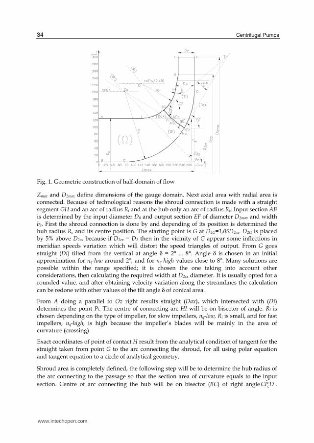
This way the domain is completely defined analytically and with the exception of point G, all connections are continuous and crossing sections from A to G are relatively constant.

a) nq=25,7 b) nq=80,8

Fig. 2. Analyzing domain with finite elements

3. Domain discretization

Integrating flow function ψ and potential velocity function ϕ is done by FEM using

quadrilateral izo-parametric linear finite elements. To maintain good accuracy in the

application of FEM it is necessary that the sides of quadrilaterals to be relatively equal in

length, that some sides are not disproportionately small compared to others.

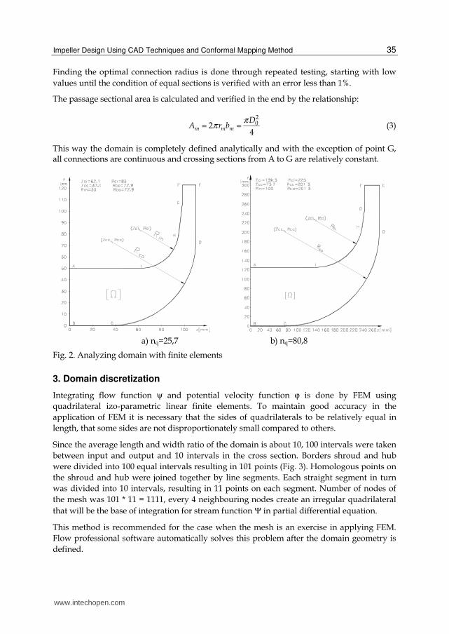
Since the average length and width ratio of the domain is about 10, 100 intervals were taken

between input and output and 10 intervals in the cross section. Borders shroud and hub

were divided into 100 equal intervals resulting in 101 points (Fig. 3). Homologous points on

the shroud and hub were joined together by line segments. Each straight segment in turn

was divided into 10 intervals, resulting in 11 points on each segment. Number of nodes of

the mesh was 101 * 11 = 1111, every 4 neighbouring nodes create an irregular quadrilateral

that will be the base of integration for stream function Ψ in partial differential equation.

This method is recommended for the case when the mesh is an exercise in applying FEM.

Flow professional software automatically solves this problem after the domain geometry is

defined.

www.intechopen.com

Centrifugal Pumps

36

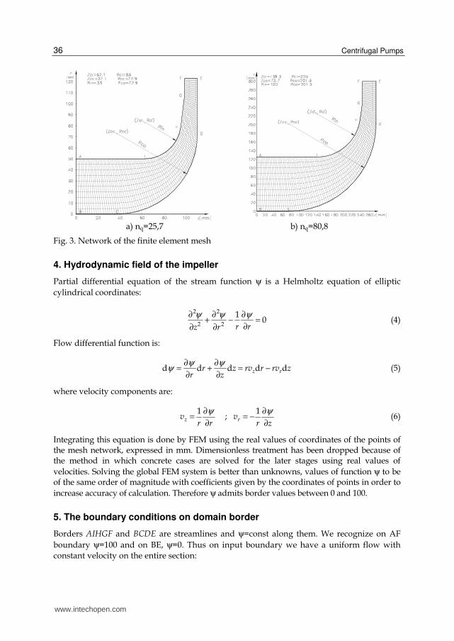
a) nq=25,7 b) nq=80,8

Fig. 3. Network of the finite element mesh

4. Hydrodynamic field of the impeller

Partial differential equation of the stream function ψ is a Helmholtz equation of elliptic

cylindrical coordinates:

2 2

2 2

10

r rz r

ψ ψ ψ∂ ∂ ∂+ − =

∂∂ ∂ (4)

Flow differential function is:

d d d d dz rr z rv r rv zr z

ψ ψψ

∂ ∂= + = −

∂ ∂ (5)

where velocity components are:

1 1

; z rv vr r r z

ψ ψ∂ ∂= = −

∂ ∂ (6)

Integrating this equation is done by FEM using the real values of coordinates of the points of the mesh network, expressed in mm. Dimensionless treatment has been dropped because of the method in which concrete cases are solved for the later stages using real values of

velocities. Solving the global FEM system is better than unknowns, values of function ψ to be of the same order of magnitude with coefficients given by the coordinates of points in order to

increase accuracy of calculation. Therefore ψ admits border values between 0 and 100.

5. The boundary conditions on domain border

Borders AIHGF and BCDE are streamlines and ψ=const along them. We recognize on AF

boundary ψ=100 and on BE, ψ=0. Thus on input boundary we have a uniform flow with

constant velocity on the entire section:

www.intechopen.com


37

20

40 ; r z

Qv v

Dπ= = (7)

Replacing (7) in (5) and integrating results:

22 20 0

4 4d

2i

Q Qr r r C

D Dψ

π π= = + (8)

Admitting that on the hub border we have ψ = 0, including the point B, will result integration constant Ci:

i( 0) ( 0) (C 0)r ψ= = = (9)

On the shroud border stream function will be constant and equal to that of point A where r=D0/2, and ψ=Q/2π=100 (quasi-unitary flow).

2 max 2

; 0r z

Qv v

D bπ= = (10)

Replacing (4.10) in (4.5) and integrating results:

2max

2

2 max 2 2

d d2

Dr

r e

Q zQrv z r z C

D b bψ

π π

== − = − = − + (11)

Admitting the same conditions on the solid boundaries result:

maxe

2

( ) ( 0) C2

E

Qzz z

bψ

π

= = = (12)

As a result, the law of variation ψ on the border EF is given by:

maxmax

2 2 2

1( )

2 2 2

QzQz Qz z

b b bψ

π π π= − + = − (13)

Integration with FEM of the Helmholtz equation (4) will be in an area where function values are imposed on border which means that we have to solve a problem of Dirichlet type.

6. Calculus of stream function Ψ by FEM

The above have created all necessary conditions for the Helmholtz equation (4) integration by FEM. Function ψ can be globally approximated on Ω by:

; 1,Gaα αψ ψ α= = (14)

where G is the number of nodes on Ω. Applying Galerkin's method (Anton at al. 1988) follows:

2 2

2 2

1d 0a

r rz rα

ψ ψ ψΩ

∂ ∂ ∂+ − Ω = ∂∂ ∂ (15)

www.intechopen.com

Centrifugal Pumps

38

Using the notation (Anton at al. 1988) resolution is reduced to solving the global linear system of equations:

where , 1,D F Gαβ β αψ α β= = (16)

The method of solving the system can be Gauss-Seidel iterative method, resulting in final

values of the stream function ψ mesh nodes. From a mathematical point of view the lines are defined by the geometrical locus of points where the stream function has the same values. If

between the solid borders the stream function ψ takes values between 0 and 100, then

streamlines having ψ = 10, 20,..., 90 are looked for because ψ = 0 and ψ = 100 are the solid borders. Identification of the points for stream lines is made through interpolation with cubic SPLINE function to have more precision.

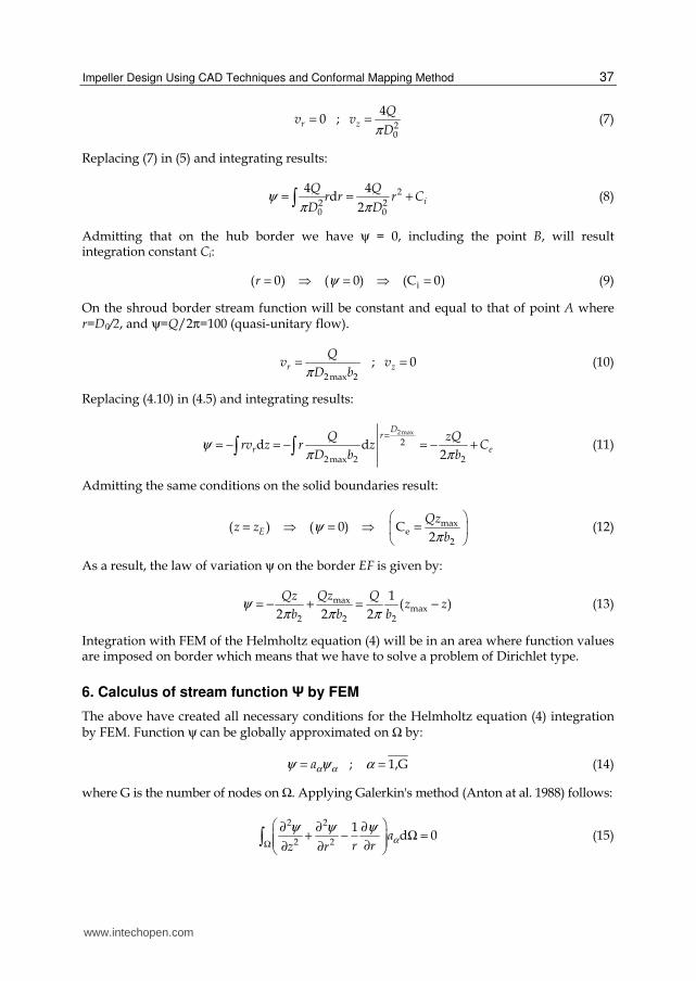
Applying the same methodology (Anton at al. 1988) as for the stream function ψ can

integrate the equation for the velocity potential function, ϕ, in the end getting equipotential lines that overlap the stream lines as shown in Fig. 4.

a) nq=25,7 b) nq=80,8

Fig. 4. Stream and equipotential lines of the hydrodynamic spectrum

7. Determination of the velocities and pressures fields

Taking into account relations (6) and the notation (Anton at al. 1988) meridian velocity

components in the centre of gravity of each finite element are calculated with relations:

20 2

10 2

4

4

e ez N N

e er N N

v Aa

v Aa

ψα

ψα

= =

(17)

Meridians speed module will be calculated with the relationship:

( ) ( )2 2

e e em z rv v v= + (18)

www.intechopen.com


39

Speed on borders is calculated by extrapolation. When calculating the pressure a Bernoulli equation is applied along a stream lines, between a point on the inlet border and a current point on the domain, points belonging to the same stream line. If on the boundary AB velocity is constant and equal with v0 and pressure p is p0 we have the Bernoulli equation:

( )2 20 0

2mp p v v

ρ= + − (19)

Dividing the current speeds and pressures with p0 and v0 so that we form dimensionless calculation:

0

mm

vv

v= (20)

( )2

020

1

2

p m

p pp C v

vρ

−= = = − (21)

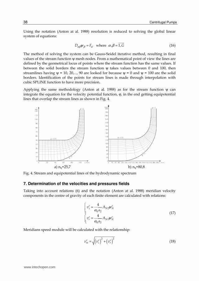
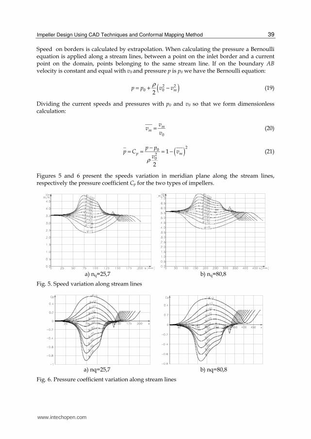
Figures 5 and 6 present the speeds variation in meridian plane along the stream lines, respectively the pressure coefficient Cp for the two types of impellers.

a) nq=25,7 b) nq=80,8

Fig. 5. Speed variation along stream lines

a) nq=25,7 b) nq=80,8

Fig. 6. Pressure coefficient variation along stream lines

www.intechopen.com

Centrifugal Pumps

40

8. Choosing the blade area in the domain of hydrodynamic field

Classic calculus relations and design method are combined with facilities of computer use in this phase. Meridian hydrodynamic field data in an optimized domain depending of impeller type offers the perspective of results close to reality. Sections of the calculation are equal to the number of stream lines (11 lines of flow) which means doubling or even tripling them to the case of using the graphic-analytical method of tracing the hydrodynamic field.

Choice of blade area in as many variations or options initially imposed is an additional possibility to optimize the blades.

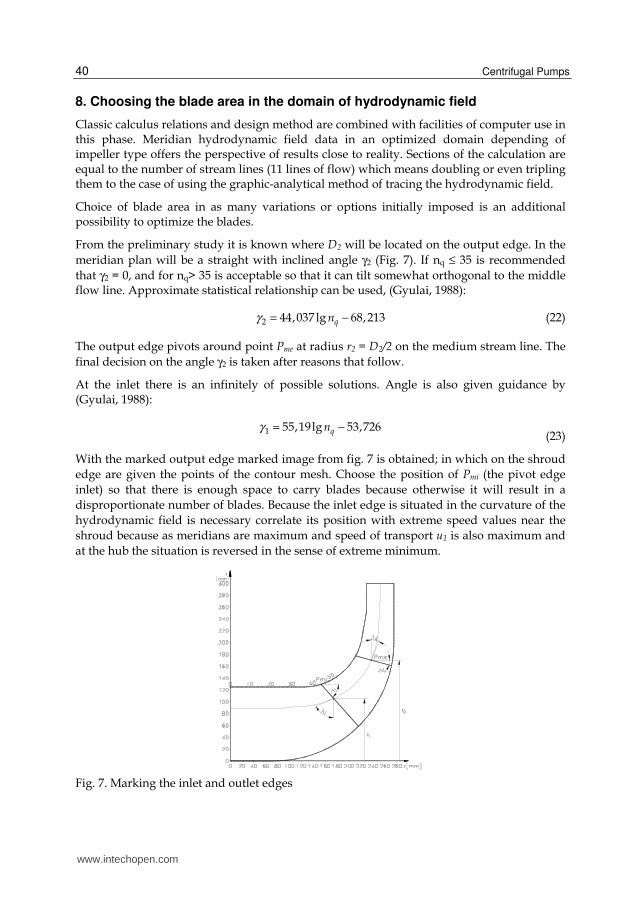
From the preliminary study it is known where D2 will be located on the output edge. In the

meridian plan will be a straight with inclined angle γ2 (Fig. 7). If nq ≤ 35 is recommended

that γ2 = 0, and for nq> 35 is acceptable so that it can tilt somewhat orthogonal to the middle flow line. Approximate statistical relationship can be used, (Gyulai, 1988):

2 44,037 lg 68,213qnγ = − (22)

The output edge pivots around point Pme at radius r2 = D2/2 on the medium stream line. The

final decision on the angle γ2 is taken after reasons that follow.

At the inlet there is an infinitely of possible solutions. Angle is also given guidance by (Gyulai, 1988):

1 55,19lg 53,726qnγ = −

(23)

With the marked output edge marked image from fig. 7 is obtained; in which on the shroud

edge are given the points of the contour mesh. Choose the position of Pmi (the pivot edge

inlet) so that there is enough space to carry blades because otherwise it will result in a

disproportionate number of blades. Because the inlet edge is situated in the curvature of the

hydrodynamic field is necessary correlate its position with extreme speed values near the

shroud because as meridians are maximum and speed of transport u1 is also maximum and

at the hub the situation is reversed in the sense of extreme minimum.

Fig. 7. Marking the inlet and outlet edges

www.intechopen.com


41

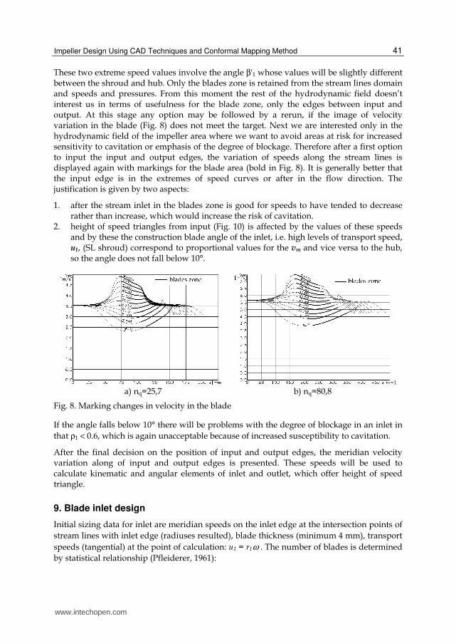
These two extreme speed values involve the angle β'1 whose values will be slightly different between the shroud and hub. Only the blades zone is retained from the stream lines domain and speeds and pressures. From this moment the rest of the hydrodynamic field doesn’t interest us in terms of usefulness for the blade zone, only the edges between input and output. At this stage any option may be followed by a rerun, if the image of velocity variation in the blade (Fig. 8) does not meet the target. Next we are interested only in the hydrodynamic field of the impeller area where we want to avoid areas at risk for increased sensitivity to cavitation or emphasis of the degree of blockage. Therefore after a first option to input the input and output edges, the variation of speeds along the stream lines is displayed again with markings for the blade area (bold in Fig. 8). It is generally better that the input edge is in the extremes of speed curves or after in the flow direction. The justification is given by two aspects:

1. after the stream inlet in the blades zone is good for speeds to have tended to decrease rather than increase, which would increase the risk of cavitation.

2. height of speed triangles from input (Fig. 10) is affected by the values of these speeds and by these the construction blade angle of the inlet, i.e. high levels of transport speed, u1, (SL shroud) correspond to proportional values for the vm and vice versa to the hub, so the angle does not fall below 10°.

a) nq=25,7 b) nq=80,8

Fig. 8. Marking changes in velocity in the blade

If the angle falls below 10° there will be problems with the degree of blockage in an inlet in

that ρ1 < 0.6, which is again unacceptable because of increased susceptibility to cavitation.

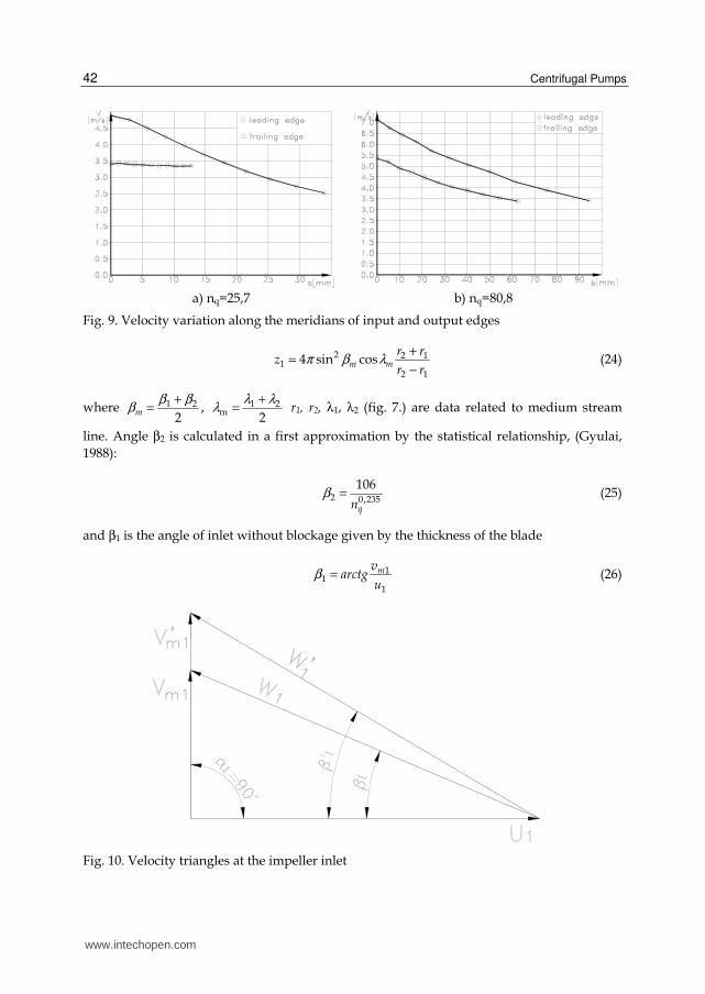
After the final decision on the position of input and output edges, the meridian velocity variation along of input and output edges is presented. These speeds will be used to calculate kinematic and angular elements of inlet and outlet, which offer height of speed triangle.

9. Blade inlet design

Initial sizing data for inlet are meridian speeds on the inlet edge at the intersection points of

stream lines with inlet edge (radiuses resulted), blade thickness (minimum 4 mm), transport

speeds (tangential) at the point of calculation: u1 = r1ω . The number of blades is determined

by statistical relationship (Pfleiderer, 1961):

www.intechopen.com

Centrifugal Pumps

42

a) nq=25,7 b) nq=80,8

Fig. 9. Velocity variation along the meridians of input and output edges

2 2 11

2 1

4 sin cosm m

r rz

r rπ β λ

+=

− (24)

where 1 2 1 2m,

2 2m

β β λ λβ λ

+ += = r1, r2, λ1, λ2 (fig. 7.) are data related to medium stream

line. Angle β2 is calculated in a first approximation by the statistical relationship, (Gyulai,

1988):

2 0,235

106

qnβ = (25)

and β1 is the angle of inlet without blockage given by the thickness of the blade

11

1

mvarctg

uβ = (26)

Fig. 10. Velocity triangles at the impeller inlet

www.intechopen.com


43

Section B-B (zoom)

Detail A

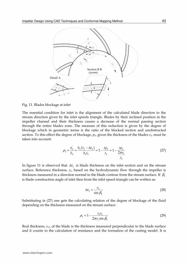
Fig. 11. Blades blockage at inlet

The essential condition for inlet is the alignment of the calculated blade direction to the stream direction given by the inlet speeds triangle. Blades by their inclined position in the impeller channel and their thickness causes a decrease of the normal passing section through the entire blades zone. The measure of this reduction is given by the degree of blockage which in geometric terms is the ratio of the blocked section and unobstructed

section. To this effect the degree of blockage, ρ1, given the thickness of the blades s1, must be taken into account:

( )'

1 1 11 1 11

11 1 1 1

1

1 12

b t tS t t

rS b t tz

ρπ

− Δ Δ Δ= = = − = − (27)

In figure 11 is observed that 1tΔ is blade thickness on the inlet section and on the stream

surface. Reference thickness, s1, based on the hydrodynamic flow through the impeller is

thickness measured in a direction normal to the blade contour from the stream surface. If '1β

is blade construction angle of inlet then from the inlet speed triangle can be written as:

11 '

1sin

st

βΔ = (28)

Substituting in (27) one gets the calculating relation of the degree of blockage of the fluid depending on the thickness measured on the stream surface:

1 11 '

1 1

12 sin

z s

rρ

π β= − (29)

Real thickness, s1r, of the blade is the thickness measured perpendicular to the blade surface and it counts in the calculation of resistance and the formation of the casting model. It is

www.intechopen.com

Centrifugal Pumps

44

highlighted under section B - B in Fig. 11 and is calculated based on the tilting of the blade surface to the plane tangent to the flow surface at the point of view, tilt angle estimated by

1ε , so that:

1 1 1sinrs s ε= ⋅ (30)

The degree of blockage depending on real thickness is calculated by the relationship:

1 11 '

1 1 1

12 sin sin

rz s

rρ

π β ε= −

⋅ ⋅ (31)

Relation (31) resulted in geometric terms. Using a result of the continuity relationship (flow

volume) will result the link of the blockage degree with the cinematic elements of inlet,

(speeds). Having no ante-stator, normal inlet is considered, α1 = 90°, (Fig. 10). Meridian

speed with blockage is calculated under the formula:

, 11

1

mm

vv

ρ= (32)

then the resulting angle of blades construction at inlet:

,

' 1 111

1 11 1'

1 1 1

12 sin sin

m

r

tg tgvarctg arctg arctg

z su

r

β ββ

ρπ β ε

= = =−

⋅ ⋅

(33)

If in relation (33) '1mv is replaced with (32) or ρ1 with (31) we get a default formula for '

1β . Its

solution is obtained through an iterative calculation initiated by an approximated value of ρ1

(ρ1 = 0.8). The resulting array is fast converging to the sought value.

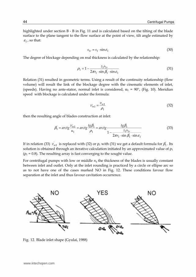
For centrifugal pumps with low or middle nq the thickness of the blades is usually constant

between inlet and outlet. Only at the inlet rounding is practiced by a circle or ellipse arc so

as to not have one of the cases marked NO in Fig. 12. These conditions favour flow

separation at the inlet and thus favour cavitation occurrence.

Fig. 12. Blade inlet shape (Gyulai, 1988)

www.intechopen.com


45

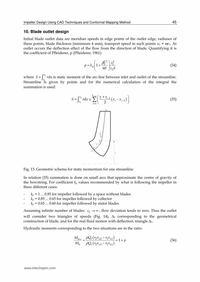
10. Blade outlet design

Initial blade outlet data are meridian speeds in edge points of the outlet edge, radiuses of

these points, blade thickness (minimum 4 mm), transport speed in such points u2 = ωr2. At outlet occurs the deflection effect of the flow from the direction of blade. Quantifying it is the coefficient of Pfleiderer, p (Pfleiderer, 1961):

[ ] 2

22

2

160

p

rp k

z S

β ° = + (34)

where 2

1

dxx

xS r= is static moment of the arc-line between inlet and outlet of the streamline.

Streamline is given by points and for the numerical calculation of the integral the

summation is used:

( )max

2

1

11

1

d2

Ix i i

i ixi

r rS r x x x−

−=

+ = ≅ − (35)

Fig. 13. Geometric schema for static momentum for one streamline

In relation (35) summation is done on small arcs that approximate the centre of gravity of the bowstring. For coefficient kp values recommended by what is following the impeller in three different cases:

- kp = 1 ... 0.85 for impeller followed by a space without blades - kp = 0.85 ... 0.65 for impeller followed by collector - kp = 0.65 ... 0.60 for impeller followed by stator blades

Assuming infinite number of blades: 2z → ∞ , flow deviation tends to zero. Thus the outlet

will consider two triangles of speeds (Fig. 14), Δ2 corresponding to the geometrical

construction of blade, and for the real fluid motion with deflection, triangle Δ3.

Hydraulic moments corresponding to the two situations are in the ratio:

( )( )

2 2 1 1

2 3 1 1

1t u uh

h t u u

Q r v r vMp

M Q r v r v

ρ

ρ∞ −

= = +−

(36)

www.intechopen.com

Centrifugal Pumps

46

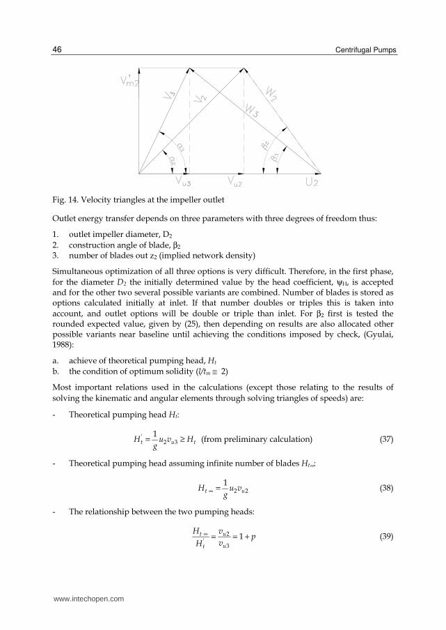
Fig. 14. Velocity triangles at the impeller outlet

Outlet energy transfer depends on three parameters with three degrees of freedom thus:

1. outlet impeller diameter, D2

2. construction angle of blade, β2 3. number of blades out z2 (implied network density)

Simultaneous optimization of all three options is very difficult. Therefore, in the first phase,

for the diameter D2 the initially determined value by the head coefficient, ψH, is accepted and for the other two several possible variants are combined. Number of blades is stored as options calculated initially at inlet. If that number doubles or triples this is taken into

account, and outlet options will be double or triple than inlet. For β2 first is tested the rounded expected value, given by (25), then depending on results are also allocated other possible variants near baseline until achieving the conditions imposed by check, (Gyulai, 1988):

a. achieve of theoretical pumping head, Ht

b. the condition of optimum solidity (l/tm ≅ 2)

Most important relations used in the calculations (except those relating to the results of

solving the kinematic and angular elements through solving triangles of speeds) are:

- Theoretical pumping head Ht:

'2 3

1 (from preliminary calculation)t u tH u v H

g= ≥ (37)

- Theoretical pumping head assuming infinite number of blades Ht∞:

2 2

1t uH u v

g∞ = (38)

- The relationship between the two pumping heads:

2'

3

1t u

ut

H vp

vH∞ = = + (39)

www.intechopen.com


47

Outlet calculation is a calculation to check the "n" variants out of which the optimal variant is chosen as the best option that is closest to the initial conditions, i.e. achieving theoretical pumping head and the condition of optimum solidity (≅ 2).

11. Calculation of the blade surface in the space frame between inlet and outlet using CAD techniques

The route of inlet to outlet is resolved by interpolating one of the significant kinematic quantities for load distribution along the inter-blades channel of impeller. Interpolation is done along the streamline (flow 3D surface) controlled by curvilinear coordinate "x" and not by the current radius "r" because it better quantifies the load (load distribution) in the radial-axial zone. Hydraulic momentum is the size that reflects blade loading between inlet and outlet. For a current point of curvilinear coordinate x it says:

( )11hx t x ux uM Q r v r vρ= − (40)

From (40) specifying (rvu)x follows:

( ) 1 1 ( )hxu ux

t

Mrv r v f x

Qρ= + = (41)

Size directly related to hydraulic momentum is (rvu)x, so if the variation of product rvu along impeller channel is controlled, then results the variation of hydraulic momentum versus radius, partial pumping head distribution, distribution of pressure differences on the faces of the blade. rvu product variation implies variation of the construction angle β necessary under the assumption that the relative velocity is tangential to the middle surface of the

blade. Height of speeds triangles is given by meridian speed, 'mv , which is vm corrected with

degree of blockage, ρ1-2, resulted from thickness of the blades. If we consider a current point on streamline denoted by "i", then current angle βi is resulting from the relationship:

1mi

ii i ui

varctg

u vβ

ρ

=

− (42)

It is noted that in (42) appear factors ri (ui = riω) and vui, so no matter which of the two variants are interpolated (rvu or β), we get the same kind of information. Most often angle β, is chosen, being directly related to the blade channel orientation in impeller.

β angle variation between inlet and outlet must be chosen so that there is a relatively uniform blade loading and the variation is strictly increasing throughout the area. For a better flow engage at the inlet and outlet, as stated above, it is recommended that at neighbourhood extreme points, the blade loading tend to zero. Analyzing several cases of impellers that condition is satisfied if the curve of β variation have derived zero at inlet and outlet. Computer solving is possible only through an analytical generation.

11.1 β angle interpolation with two connected parabola arcs

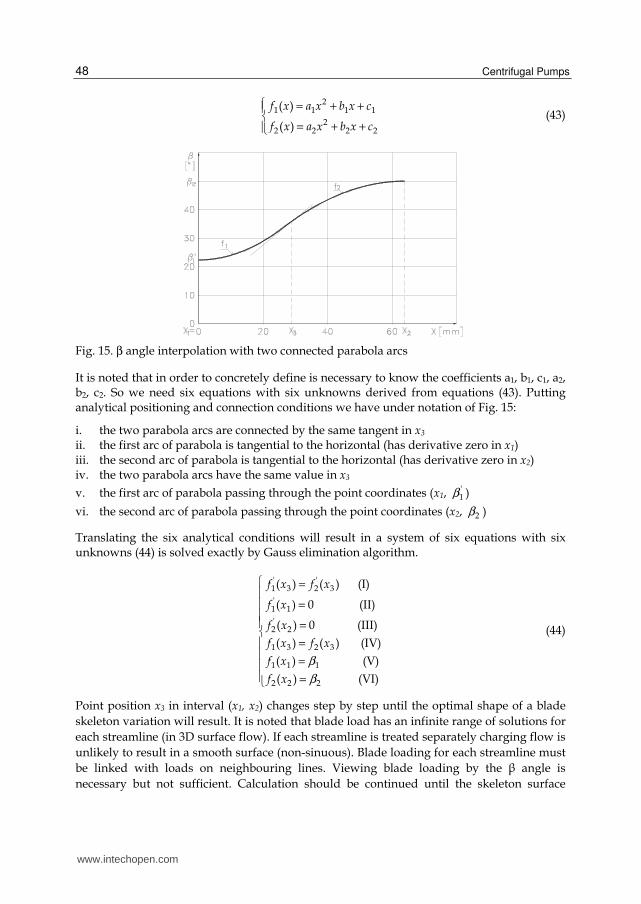
Connecting the two arcs of parabola is the point x3 as common tangent (Fig.15). Functions that define two parabola arcs with vertical focal axis noted by f1 and f2 with general equations, (Milos, 2009):

www.intechopen.com

Centrifugal Pumps

48

2

1 1 1 1

22 2 2 2

( )

( )

f x a x b x c

f x a x b x c

= + += + + (43)

Fig. 15. β angle interpolation with two connected parabola arcs

It is noted that in order to concretely define is necessary to know the coefficients a1, b1, c1, a2, b2, c2. So we need six equations with six unknowns derived from equations (43). Putting analytical positioning and connection conditions we have under notation of Fig. 15:

i. the two parabola arcs are connected by the same tangent in x3 ii. the first arc of parabola is tangential to the horizontal (has derivative zero in x1) iii. the second arc of parabola is tangential to the horizontal (has derivative zero in x2) iv. the two parabola arcs have the same value in x3

v. the first arc of parabola passing through the point coordinates (x1, '1β )

vi. the second arc of parabola passing through the point coordinates (x2, 2β )

Translating the six analytical conditions will result in a system of six equations with six unknowns (44) is solved exactly by Gauss elimination algorithm.

' '1 3 2 3

'1 1

'2 2

1 3 2 3

1 1 1

2 2 2

( ) ( ) (I)

( ) 0 (II)

( ) 0 (III)

( ) ( ) (IV)

( ) (V)

( ) (VI)

f x f x

f x

f x

f x f x

f x

f x

β

β

== === =

(44)

Point position x3 in interval (x1, x2) changes step by step until the optimal shape of a blade

skeleton variation will result. It is noted that blade load has an infinite range of solutions for

each streamline (in 3D surface flow). If each streamline is treated separately charging flow is

unlikely to result in a smooth surface (non-sinuous). Blade loading for each streamline must

be linked with loads on neighbouring lines. Viewing blade loading by the β angle is

necessary but not sufficient. Calculation should be continued until the skeleton surface

www.intechopen.com


49

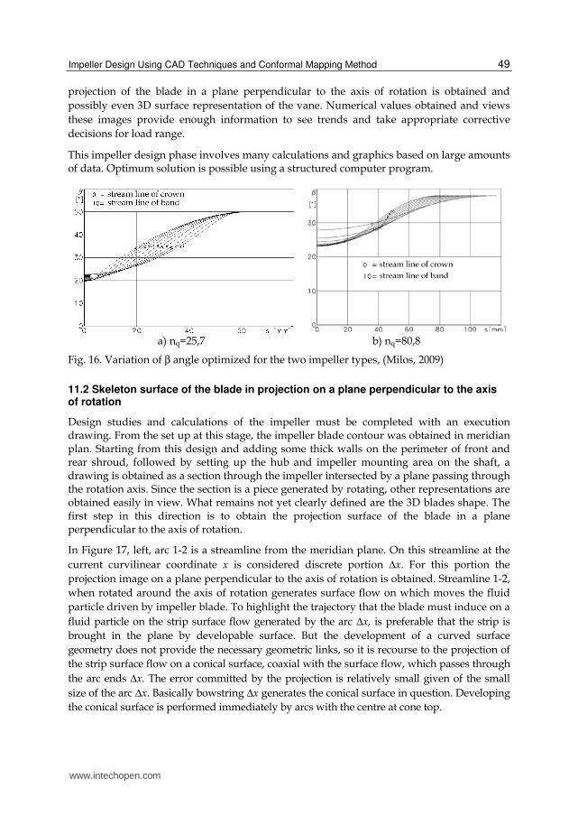
projection of the blade in a plane perpendicular to the axis of rotation is obtained and

possibly even 3D surface representation of the vane. Numerical values obtained and views

these images provide enough information to see trends and take appropriate corrective

decisions for load range.

This impeller design phase involves many calculations and graphics based on large amounts of data. Optimum solution is possible using a structured computer program.

a) nq=25,7 b) nq=80,8

Fig. 16. Variation of β angle optimized for the two impeller types, (Milos, 2009)

11.2 Skeleton surface of the blade in projection on a plane perpendicular to the axis of rotation

Design studies and calculations of the impeller must be completed with an execution drawing. From the set up at this stage, the impeller blade contour was obtained in meridian plan. Starting from this design and adding some thick walls on the perimeter of front and rear shroud, followed by setting up the hub and impeller mounting area on the shaft, a drawing is obtained as a section through the impeller intersected by a plane passing through the rotation axis. Since the section is a piece generated by rotating, other representations are obtained easily in view. What remains not yet clearly defined are the 3D blades shape. The first step in this direction is to obtain the projection surface of the blade in a plane perpendicular to the axis of rotation.

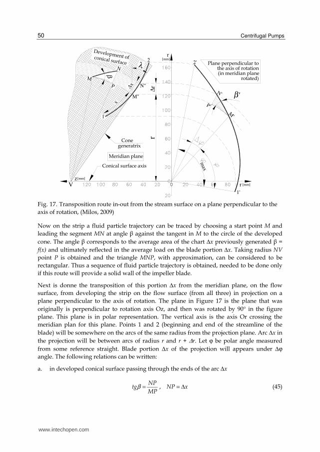
In Figure 17, left, arc 1-2 is a streamline from the meridian plane. On this streamline at the

current curvilinear coordinate x is considered discrete portion Δx. For this portion the

projection image on a plane perpendicular to the axis of rotation is obtained. Streamline 1-2,

when rotated around the axis of rotation generates surface flow on which moves the fluid

particle driven by impeller blade. To highlight the trajectory that the blade must induce on a

fluid particle on the strip surface flow generated by the arc Δx, is preferable that the strip is

brought in the plane by developable surface. But the development of a curved surface

geometry does not provide the necessary geometric links, so it is recourse to the projection of

the strip surface flow on a conical surface, coaxial with the surface flow, which passes through

the arc ends Δx. The error committed by the projection is relatively small given of the small

size of the arc Δx. Basically bowstring Δx generates the conical surface in question. Developing

the conical surface is performed immediately by arcs with the centre at cone top.

www.intechopen.com

Centrifugal Pumps

50

r[mm]

r [mm]

z[mm]

max

β'

β

λ

V

Meridian plane

Plane perpendicular to

(in meridian planerotated)

x

xΔ

N

M

P

1

2

N'

P'

M'

N"

M"

rΔ

r

Conical surface axis

2'

1'

Conegeneratrix

Development ofconical surfacethe axis of rotation

Fig. 17. Transposition route in-out from the stream surface on a plane perpendicular to the

axis of rotation, (Milos, 2009)

Now on the strip a fluid particle trajectory can be traced by choosing a start point M and

leading the segment MN at angle β against the tangent in M to the circle of the developed

cone. The angle β corresponds to the average area of the chart Δx previously generated β =

f(x) and ultimately reflected in the average load on the blade portion Δx. Taking radius NV

point P is obtained and the triangle MNP, with approximation, can be considered to be

rectangular. Thus a sequence of fluid particle trajectory is obtained, needed to be done only

if this route will provide a solid wall of the impeller blade.

Next is donne the transposition of this portion Δx from the meridian plane, on the flow

surface, from developing the strip on the flow surface (from all three) in projection on a

plane perpendicular to the axis of rotation. The plane in Figure 17 is the plane that was

originally is perpendicular to rotation axis Oz, and then was rotated by 90° in the figure

plane. This plane is in polar representation. The vertical axis is the axis Or crossing the

meridian plan for this plane. Points 1 and 2 (beginning and end of the streamline of the

blade) will be somewhere on the arcs of the same radius from the projection plane. Arc Δx in

the projection will be between arcs of radius r and r + Δr. Let ϕ be polar angle measured

from some reference straight. Blade portion Δx of the projection will appears under Δϕ

angle. The following relations can be written:

a. in developed conical surface passing through the ends of the arc Δx

NP

tgMP

β = , NP x= Δ (45)

www.intechopen.com


51

b. in the projection plane perpendicular to the axis of rotation

' '

'' '

N P rtg

rM Pβ

ϕ

Δ= =

Δ, ' 'N P r= Δ (46)

Arc MP is projected in real size, becoming M'P ', i.e.

' 'MP M P r ϕ= = Δ (47)

Replacing the first two relations we have:

x

tgr

βϕ

Δ=

Δ (48)

' cosr

tg tg tgx

β β β λΔ

= = ⋅Δ

(49)

If you go to the limit with small infinites: x dxΔ → and dϕ ϕΔ → resulting differential

equation:

dx

tgr d

βϕ

=⋅

(50)

Separating variables and integrating

1

x

x

dx

r tgϕ

β=

⋅ (51)

Integration is done along the streamline. The image in projection on a plane perpendicular to the axis of rotation is calculated and represents in the polar coordinates (r, ϕ), ϕ resulting in radians from the relation (51). To solve analytically the integral (51) there should be an analytical dependence r = r(x) and tgβ = f(x). Since often discrete values of these dependencies are available, a numerical integration method is preferred. Integration is done by adding the number of partial areas using trapezoids (Fig. 12).

1

1

1 1

2i i

i

i i

x x

r tg r tgϕ

β β+

+

−Δ = +

⋅ ⋅ (52)

Δϕi angles calculated with (52) result in radians. Adding them step by step, current wrapping angles of the middle surface of blade are obtained.

1

i

i ii

ϕ ϕ=

= Δ (53)

Thus each point (ri, zi) of the streamline is associated with an angle ϕi and results the

defining of the middle surface of the blade in cylindrical coordinates (ri, ϕi, zi)

From hydrodynamic field calculations we have 3 ... 11 or even more streamlines. Applying

relation (51) for each streamline will result ϕmax. With ϕmax you can start calculating ϕ

www.intechopen.com

Centrifugal Pumps

52

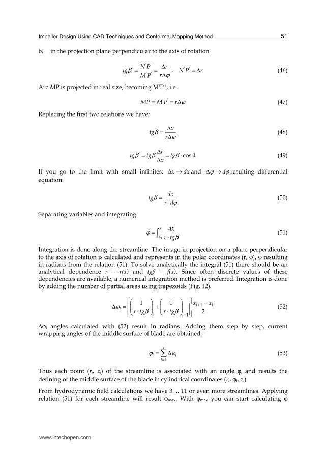
optimization which seeks to obtain all streamlines wrapping up of the same angle range.

Choosing as reference ϕmax, max angle ϕ corresponding streamline medium (line 5 in case we have 11 streamlines) using a special algorithm changes the position of points x3, position

number between 1 and 99, until maximum ϕ is the same for each streamline. For the impellers with mixed-flow shape this may not be achieved. In this case it is necessary be

provided that the differences between ϕmax are uniformly increasing or decreasing.

Fig. 18. Numerical integration of the function of wrapping angle of the blade

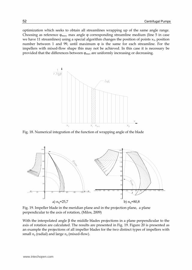
a) nq=25,7 b) nq=80,8

Fig. 19. Impeller blade in the meridian plane and in the projection plane, a plane

perpendicular to the axis of rotation, (Milos, 2009)

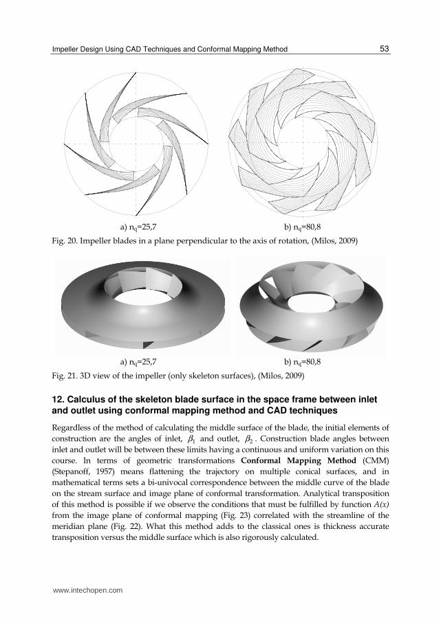
With the interpolated angle β the middle blades projections in a plane perpendicular to the axis of rotation are calculated. The results are presented in Fig. 19. Figure 20 is presented as an example the projections of all impeller blades for the two distinct types of impellers with small nq (radial) and large nq (mixed-flow).

www.intechopen.com


53

a) nq=25,7 b) nq=80,8

Fig. 20. Impeller blades in a plane perpendicular to the axis of rotation, (Milos, 2009)

a) nq=25,7 b) nq=80,8

Fig. 21. 3D view of the impeller (only skeleton surfaces), (Milos, 2009)

12. Calculus of the skeleton blade surface in the space frame between inlet

and outlet using conformal mapping method and CAD techniques

Regardless of the method of calculating the middle surface of the blade, the initial elements of

construction are the angles of inlet, 1β and outlet, 2β . Construction blade angles between

inlet and outlet will be between these limits having a continuous and uniform variation on this

course. In terms of geometric transformations Conformal Mapping Method (CMM)

(Stepanoff, 1957) means flattening the trajectory on multiple conical surfaces, and in

mathematical terms sets a bi-univocal correspondence between the middle curve of the blade

on the stream surface and image plane of conformal transformation. Analytical transposition

of this method is possible if we observe the conditions that must be fulfilled by function A(x)

from the image plane of conformal mapping (Fig. 23) correlated with the streamline of the

meridian plane (Fig. 22). What this method adds to the classical ones is thickness accurate

transposition versus the middle surface which is also rigorously calculated.

www.intechopen.com

Centrifugal Pumps

54

0

20

40

60

80

100

120

140

160

r[mm]

0 20 40 60 80 100 120 140 160 r[mm]020406080100z[mm]

20

40

max

R

R

R

xx

x

i

i+1

i

i

i med

i+1

Ai

i

i

Lm

蔕2 蔔

蔕1

蔔

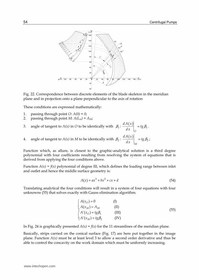
Fig. 22. Correspondence between discrete elements of the blade skeleton in the meridian plane and in projection onto a plane perpendicular to the axis of rotation

These conditions are expressed mathematically:

1. passing through point O: A(0) = 0; 2. passing through point M: A(Lm) = AM;

3. angle of tangent to A(x) in O to be identically with 1β : ( )

1

O

d A xtg

d xβ= .

4. angle of tangent to A(x) in M to be identically with 2β : ( )

2

M

d A xtg

d xβ= ;

Function which, as allure, is closest to the graphic-analytical solution is a third degree polynomial with four coefficients resulting from resolving the system of equations that is derived from applying the four conditions above.

Function A(x) = f(x) polynomial of degree III, which defines the loading range between inlet and outlet and hence the middle surface geometry is:

3 2( )A x ax bx cx d= + + + (54)

Translating analytical the four conditions will result in a system of four equations with four unknowns (55) that solves exactly with Gauss elimination algorithm.

1

2

( ) 0 (I)

( ) (II)

'( ) (III)

'( ) (IV)

O

M M

O

M

A x

A x A

A x tg

A x tg

β

β

= == =

(55)

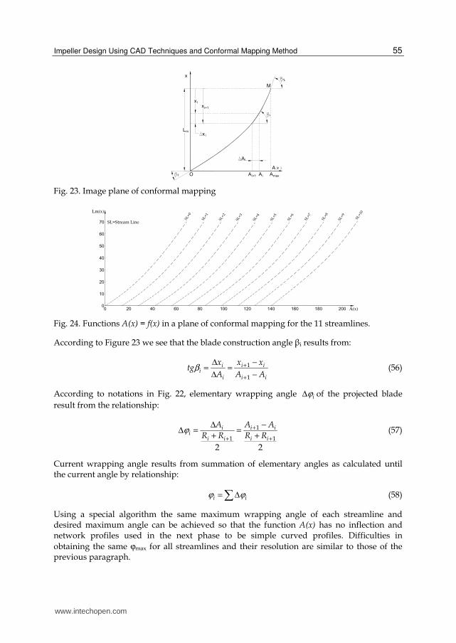
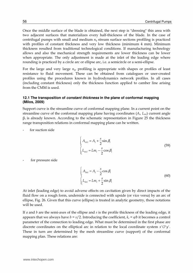
In Fig. 24 is graphically presented A(x) = f(x) for the 11 streamlines of the meridian plane.

Basically, strips carried on the conical surface (Fig. 17) are here put together in the image plane. Function A(x) must be at least level 3 to allow a second order derivative and thus be able to control the concavity on the work domain which must be uniformly increasing.

www.intechopen.com


55

L

x

A

M

AAO

xx

ii+1

m

i+1 i Amax1

2

i

蔕x 蔔

xi

Ai

Fig. 23. Image plane of conformal mapping

0

10

20

30

40

50

60

70

Lm(x)

0 20 40 60 80 100 120 140 160 180 200 A(x)

SL=

0

SL=

1

SL=

2

SL=

3

SL=

4

SL=

5

SL=

6

SL=

7

SL=

8

SL=9

SL=

10

SL=Stream Line

Fig. 24. Functions A(x) = f(x) in a plane of conformal mapping for the 11 streamlines.

According to Figure 23 we see that the blade construction angle βi results from:

1

1

i i ii

i i i

x x xtg

A A Aβ +

+

Δ −= =

Δ − (56)

According to notations in Fig. 22, elementary wrapping angle iϕΔ of the projected blade

result from the relationship:

1

1 1

2 2

i i ii

i i i i

A A A

R R R Rϕ +

+ +

Δ −Δ = =

+ + (57)

Current wrapping angle results from summation of elementary angles as calculated until the current angle by relationship:

i iϕ ϕ= Δ (58)

Using a special algorithm the same maximum wrapping angle of each streamline and desired maximum angle can be achieved so that the function A(x) has no inflection and network profiles used in the next phase to be simple curved profiles. Difficulties in

obtaining the same ϕmax for all streamlines and their resolution are similar to those of the previous paragraph.

www.intechopen.com

Centrifugal Pumps

56

Once the middle surface of the blade is obtained, the next step is "dressing" this area with two adjacent surfaces that materializes every half-thickness of the blade. In the case of centrifugal pumps with small and medium nq stream surface sections profiling is practiced with profiles of constant thickness and very low thickness (minimum 4 mm). Minimum thickness resulted from traditional technological conditions. If manufacturing technology allows and also the mechanical strength requirements are lower thickness can be lower when appropriate. The only adjustment is made at the inlet of the leading edge where rounding is practiced by a circle arc or ellipse arc, i.e. a semicircle or a semi-ellipse.

For the large and very large nq, profiling is appropriate with shapes or profiles of least

resistance to fluid movement. These can be obtained from catalogues or user-created

profiles using the procedures known in hydrodynamics network profiles. In all cases

(including constant thickness) only the thickness function applied to camber line arising

from the CMM is used.

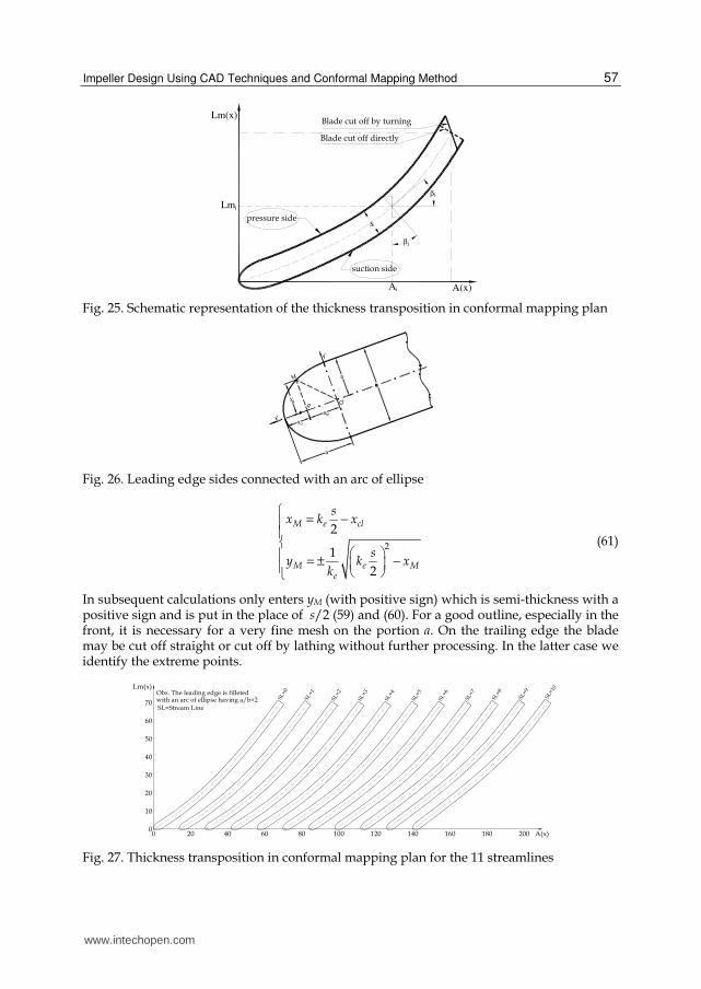
12.1 The transposition of constant thickness in the plane of conformal mapping (Milos, 2009)

Support curve is the streamline curve of conformal mapping plane. In a current point on the

streamline curve of the conformal mapping plane having coordinates (Ai, Lmi) current angle

βi is already known. According to the schematic representation in Figure 25 the thickness

range transposition relations in conformal mapping plane can be written.

- for suction side

sin2

cos2

exi i i

exi i i

sA A

sL Lm

β

β

= + = −

(59)

- for pressure side

cos

2

sin2

ini i i

ini i i

sA A

sL Lm

β

β

= − = +

(60)

At inlet (leading edge) to avoid adverse effects on cavitation given by direct impacts of the

fluid flow on a rough form, underside is connected with upside (or vice versa) by an arc of

ellipse, Fig. 26. Given that this curve (ellipse) is treated in analytic geometry, those notations

will be used.

If a and b are the semi-axes of the ellipse and s is the profile thickness of the leading edge, it

appears that we always have b = s/2. Introducing the coefficient, ke = a/b it becomes a control

parameter of the connection to leading edge. What must be determined in the first phase are

discrete coordinates on the elliptical arc in relation to the local coordinate system x'O'y'.

These in turn are determined by the mesh streamline curve (support) of the conformal

mapping plan. These relations are:

www.intechopen.com


57

βi

βi

Lm(x)

A(x)

s

A

Lm

i

i

Blade cut off by turning

Blade cut off directly

pressure side

suction side

Fig. 25. Schematic representation of the thickness transposition in conformal mapping plan

bs

xx

a

y

x'

y'

P

M

O'

cl

M

M

Fig. 26. Leading edge sides connected with an arc of ellipse

2

2

1

2

M e cl

M e Me

sx k x

sy k x

k

= − = ± −

(61)

In subsequent calculations only enters yM (with positive sign) which is semi-thickness with a positive sign and is put in the place of s/2 (59) and (60). For a good outline, especially in the front, it is necessary for a very fine mesh on the portion a. On the trailing edge the blade may be cut off straight or cut off by lathing without further processing. In the latter case we identify the extreme points.

0

10

20

30

40

50

60

70

Lm(x)

0 20 40 60 80 100 120 140 160 180 200 A(x)

SL

=0

SL

=1

SL=

2

SL

=3

SL

=4

SL=

5

SL=

6

SL=

7

SL=

8

SL=

9

SL=

10

Obs. The leading edge is filletedwith an arc of ellipse having a/b=2

SL=Stream Line

Fig. 27. Thickness transposition in conformal mapping plan for the 11 streamlines

www.intechopen.com

Centrifugal Pumps

58

For example shown in Fig. 27, results for a radial impeller thickness transposition studied in this respect.

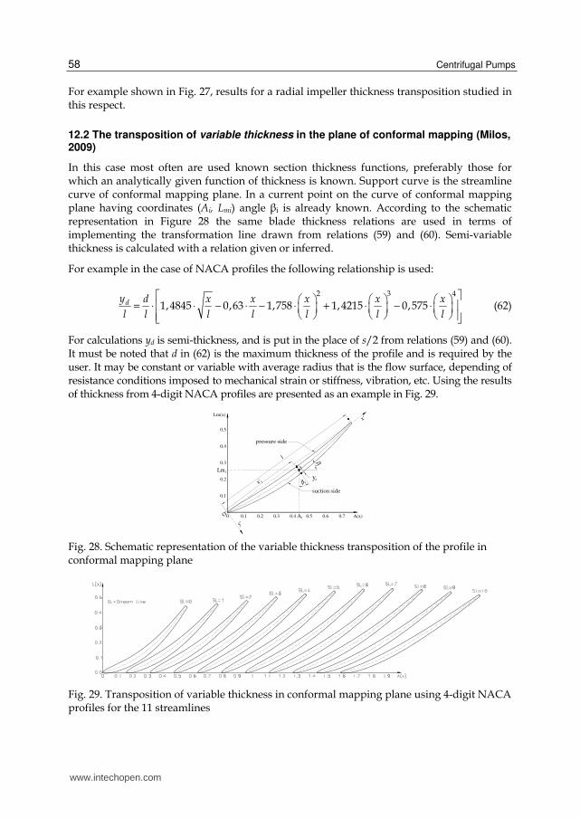
12.2 The transposition of variable thickness in the plane of conformal mapping (Milos, 2009)

In this case most often are used known section thickness functions, preferably those for which an analytically given function of thickness is known. Support curve is the streamline curve of conformal mapping plane. In a current point on the curve of conformal mapping plane having coordinates (Ai, Lmi) angle βi is already known. According to the schematic representation in Figure 28 the same blade thickness relations are used in terms of implementing the transformation line drawn from relations (59) and (60). Semi-variable thickness is calculated with a relation given or inferred.

For example in the case of NACA profiles the following relationship is used:

2 3 4

1,4845 0,63 1,758 1,4215 0,575dy d x x x x x

l l l l l l l

= ⋅ ⋅ − ⋅ − ⋅ + ⋅ − ⋅ (62)

For calculations yd is semi-thickness, and is put in the place of s/2 from relations (59) and (60). It must be noted that d in (62) is the maximum thickness of the profile and is required by the user. It may be constant or variable with average radius that is the flow surface, depending of resistance conditions imposed to mechanical strain or stiffness, vibration, etc. Using the results of thickness from 4-digit NACA profiles are presented as an example in Fig. 29.

0.1

0.2

0.3

0.4

0.5

Lm(x)

0 0.1 0.2 0.3 0.4 0.5 0.6 0.7 A(x)

yd

x'

y'

l

x'

A

Lm

i

i

O'

pressure side

suction side

i

β ii

β

Fig. 28. Schematic representation of the variable thickness transposition of the profile in conformal mapping plane

Fig. 29. Transposition of variable thickness in conformal mapping plane using 4-digit NACA profiles for the 11 streamlines

www.intechopen.com


59

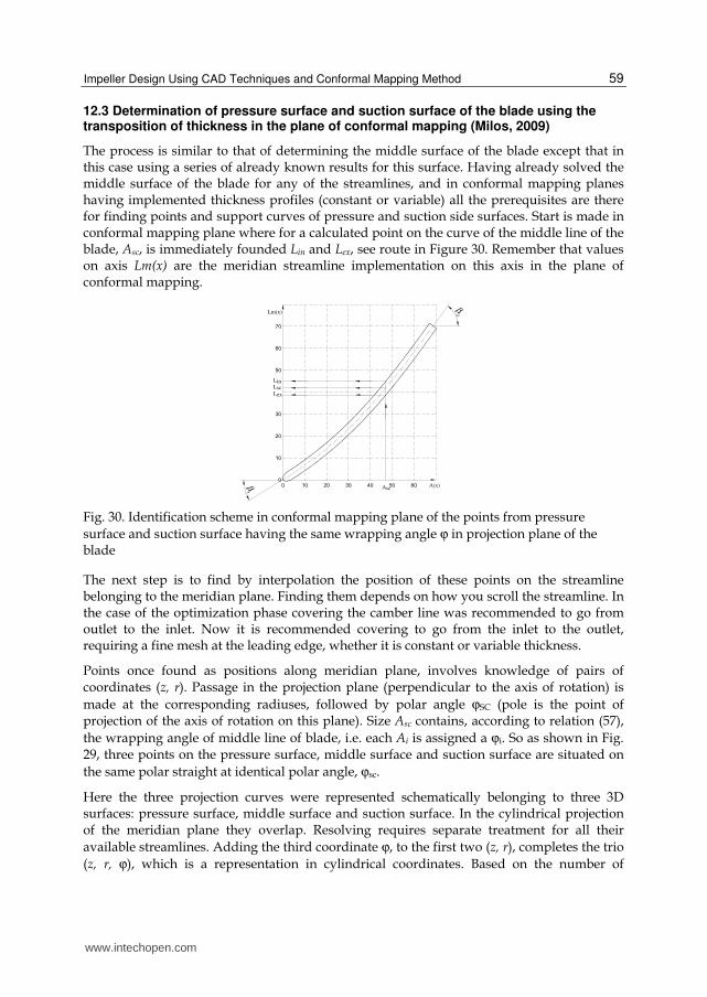
12.3 Determination of pressure surface and suction surface of the blade using the transposition of thickness in the plane of conformal mapping (Milos, 2009)

The process is similar to that of determining the middle surface of the blade except that in this case using a series of already known results for this surface. Having already solved the middle surface of the blade for any of the streamlines, and in conformal mapping planes having implemented thickness profiles (constant or variable) all the prerequisites are there for finding points and support curves of pressure and suction side surfaces. Start is made in conformal mapping plane where for a calculated point on the curve of the middle line of the blade, Asc, is immediately founded Lin and Lex, see route in Figure 30. Remember that values on axis Lm(x) are the meridian streamline implementation on this axis in the plane of conformal mapping.

0

10

20

30

50

60

70

Lm(x)

0 10 20 30 40 50 60 A(x)

β

β

2

1

LinLscLex

Asc

Fig. 30. Identification scheme in conformal mapping plane of the points from pressure

surface and suction surface having the same wrapping angle ϕ in projection plane of the blade

The next step is to find by interpolation the position of these points on the streamline belonging to the meridian plane. Finding them depends on how you scroll the streamline. In the case of the optimization phase covering the camber line was recommended to go from outlet to the inlet. Now it is recommended covering to go from the inlet to the outlet, requiring a fine mesh at the leading edge, whether it is constant or variable thickness.

Points once found as positions along meridian plane, involves knowledge of pairs of coordinates (z, r). Passage in the projection plane (perpendicular to the axis of rotation) is

made at the corresponding radiuses, followed by polar angle ϕSC (pole is the point of projection of the axis of rotation on this plane). Size Asc contains, according to relation (57),

the wrapping angle of middle line of blade, i.e. each Ai is assigned a ϕi. So as shown in Fig. 29, three points on the pressure surface, middle surface and suction surface are situated on

the same polar straight at identical polar angle, ϕsc.

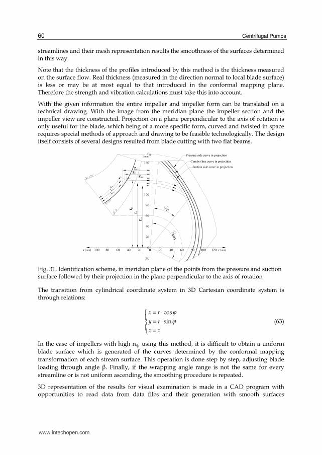
Here the three projection curves were represented schematically belonging to three 3D surfaces: pressure surface, middle surface and suction surface. In the cylindrical projection of the meridian plane they overlap. Resolving requires separate treatment for all their

available streamlines. Adding the third coordinate ϕ, to the first two (z, r), completes the trio

(z, r, ϕ), which is a representation in cylindrical coordinates. Based on the number of

www.intechopen.com

Centrifugal Pumps

60

streamlines and their mesh representation results the smoothness of the surfaces determined in this way.

Note that the thickness of the profiles introduced by this method is the thickness measured on the surface flow. Real thickness (measured in the direction normal to local blade surface) is less or may be at most equal to that introduced in the conformal mapping plane. Therefore the strength and vibration calculations must take this into account.

With the given information the entire impeller and impeller form can be translated on a technical drawing. With the image from the meridian plane the impeller section and the impeller view are constructed. Projection on a plane perpendicular to the axis of rotation is only useful for the blade, which being of a more specific form, curved and twisted in space requires special methods of approach and drawing to be feasible technologically. The design itself consists of several designs resulted from blade cutting with two flat beams.

0

20

40

60

80

100

160

r[mm]

20 40 60 80 100 120 r [mm]020406080100z [mm]

max

cl

Pressure side curve in projection

Cumber line curve in projection

Suction side curve in projection

L

LL

ex

cl

in

rr

r

ex

cl

in

zzz

in

cl

ex

Fig. 31. Identification scheme, in meridian plane of the points from the pressure and suction surface followed by their projection in the plane perpendicular to the axis of rotation

The transition from cylindrical coordinate system in 3D Cartesian coordinate system is through relations:

cos

sin

x r

y r

z z

ϕ

ϕ

= ⋅= ⋅ =

(63)

In the case of impellers with high nq, using this method, it is difficult to obtain a uniform

blade surface which is generated of the curves determined by the conformal mapping

transformation of each stream surface. This operation is done step by step, adjusting blade

loading through angle β. Finally, if the wrapping angle range is not the same for every

streamline or is not uniform ascending, the smoothing procedure is repeated.

3D representation of the results for visual examination is made in a CAD program with opportunities to read data from data files and their generation with smooth surfaces

www.intechopen.com


61

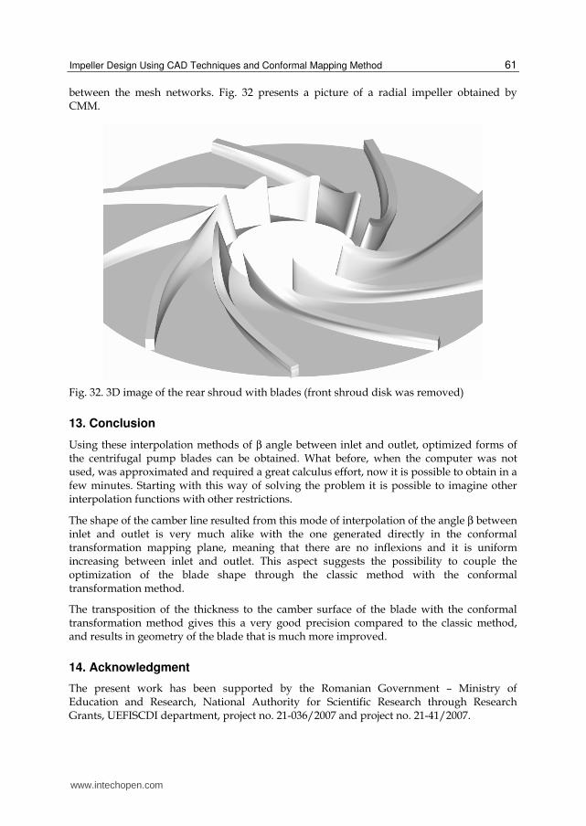
between the mesh networks. Fig. 32 presents a picture of a radial impeller obtained by CMM.

Fig. 32. 3D image of the rear shroud with blades (front shroud disk was removed)

13. Conclusion

Using these interpolation methods of β angle between inlet and outlet, optimized forms of the centrifugal pump blades can be obtained. What before, when the computer was not used, was approximated and required a great calculus effort, now it is possible to obtain in a few minutes. Starting with this way of solving the problem it is possible to imagine other interpolation functions with other restrictions.

The shape of the camber line resulted from this mode of interpolation of the angle β between inlet and outlet is very much alike with the one generated directly in the conformal transformation mapping plane, meaning that there are no inflexions and it is uniform increasing between inlet and outlet. This aspect suggests the possibility to couple the optimization of the blade shape through the classic method with the conformal transformation method.

The transposition of the thickness to the camber surface of the blade with the conformal transformation method gives this a very good precision compared to the classic method, and results in geometry of the blade that is much more improved.

14. Acknowledgment

The present work has been supported by the Romanian Government – Ministry of Education and Research, National Authority for Scientific Research through Research Grants, UEFISCDI department, project no. 21-036/2007 and project no. 21-41/2007.

www.intechopen.com

Centrifugal Pumps

62

15. References

Anton I., Câmpian V., Carte I., (1988), Hidrodinamica turbinelor bulb şi a turbinelor pompe bulb, Editura Tehnică, Bucureşti.

Anton L.E., Miloş T., (1998), Centrifugal Pumps with Inducer, Publishing house Orizonturi universitare, Timişoara, Romania, ISBN 978-973-625-838-1.

Gülich J.F., (2008), Centrifugal Pumps, Springer-Verlag Berlin Heidelberg New York, ISBN 978-3-540-73694-3.

Gyulai Fr., (1988), Pumps, Fans, Compressors; vol I & II, Publishing house of Politehnica University, Timişoara.

Miloş T., (2002), Computer Aided Optimization of Vanes Shape for Centrifugal Pump Impellers, Scientific Bulletin of The “Politehnica” University of Timişoara, Romania, Transactions on Mechanics, Tom 47(61), Fasc. 1, pp. 37-44, ISSN-1224-6077.

Miloş T., (2007), Method to Smooth the 3d Surface of the Blades of Francis Turbine Runner, International Review of Mechanical Engineering (IREME), Vol. 1, No. 6, pp. 603-607, PRAISE WORTHY PRIZE S.r.l, Publishing House, ISSN 1970-8734.

Miloş T., (2008), CAD Procedure For Blade Design of Centrifugal Pump Impeller Using Conformal Mapping Method, Fifth Conference of the Water-Power Engineering in Romania, Published in Scientific Bulletin of University POLITEHNICA of Bucharest, Series D, Mechanical Engineering, Vol.70/2008, No. 4, ISSN 1454-2358. pp. 213-220.

Miloş T., (2009), Centrifugal and Axial Pumps and Fans, Publishing house of Politehnica University, Timisoara, ISBN 978-973-625-838-1.

Miloş T., (2009), Optimal Blade Design of Centrifugal Pump Impeller Using CAD Procedures and Conformal Mapping Method, International Review of Mechanical Engineering (IREME), Vol. 3, No. 6, pp. 733-738, PRAISE WORTHY PRIZE S.r.l, Publishing House, ISSN 1970-8734.

Miloş T., Muntean S., Stuparu A., Baya A., Susan-Resiga R., (2006), Automated Procedure for Design and 3D Numerical Analysis of the Flow Through Impellers, In Proceedings of the 2nd German – Romanian Workshop on Vortex Dynamics, Stuttgart 10-14 May 2006. pp. 1-10. (on CD-ROM).

Pfleiderer K., (1961), Die Kreiselpumpen für Flüssigkeiten und Gase, Springer Verlag, Berlin. Radha Krishna H.C. (Editor), (1997), Hydraulic Design of Hydraulic Machinery, Avebury,

Ashghate Publishing Limited, ISBN: 0-29139-851-0. Stepanoff A. J., (1957), Centrifugal and Axial Flow Pumps, 2nd edition, John Wiley and Sons,

Inc., New York. Tuzson J., (2000), Centrifugal Pump Design, John Wiley & Sons, ISBN 9780471361008.

www.intechopen.com

Centrifugal PumpsEdited by Dr. Dimitris Papantonis

ISBN 978-953-51-0051-5Hard cover, 106 pagesPublisher InTechPublished online 24, February, 2012Published in print edition February, 2012

InTech EuropeUniversity Campus STeP Ri Slavka Krautzeka 83/A 51000 Rijeka, Croatia Phone: +385 (51) 770 447 Fax: +385 (51) 686 166www.intechopen.com

InTech ChinaUnit 405, Office Block, Hotel Equatorial Shanghai No.65, Yan An Road (West), Shanghai, 200040, China

Phone: +86-21-62489820 Fax: +86-21-62489821

The structure of a hydraulic machine, as a centrifugal pump, is evolved principally to satisfy the requirementsof the fluid flow. However taking into account the strong interaction between the pump and the pumpinginstallation, the need to control the operation, the requirement to operate at best efficiency in order to saveenergy, the provision to improve the operation against cavitation and other more specific but very interestingand important topics, the object of a book on centrifugal pumps must cover a large field. The present bookexamines a number of these more specific topics, beyond the contents of a textbook, treating not only thepump's design and operation but also strategies to increase energy efficiency, the fluid flow control, the faultdiagnosis.

How to referenceIn order to correctly reference this scholarly work, feel free to copy and paste the following:

Milos Teodor (2012). Impeller Design Using CAD Techniques and Conformal Mapping Method, CentrifugalPumps, Dr. Dimitris Papantonis (Ed.), ISBN: 978-953-51-0051-5, InTech, Available from:http://www.intechopen.com/books/centrifugal-pumps/impeller-design-using-cad-techniques-and-conformal-mapping-method

© 2012 The Author(s). Licensee IntechOpen. This is an open access articledistributed under the terms of the Creative Commons Attribution 3.0License, which permits unrestricted use, distribution, and reproduction inany medium, provided the original work is properly cited.

http://creativecommons.org/licenses/by/3.0

impeller design using cad techniques and conformal mapping ... · impeller design using cad...

Documents