imperfect production inventory model with …
TRANSCRIPT

Decision Making: Applications in Management and Engineering Vol. 3, Issue 2, 2020, pp. 1-18. ISSN: 2560-6018 eISSN: 2620-0104
DOI: https://doi.org/10.31181/dmame2003102g
* Corresponding author. E-mail addresses: [email protected] (P.K. Ghosh), [email protected]
(J.K. Dey)
IMPERFECT PRODUCTION INVENTORY MODEL WITH UNCERTAIN ELAPSED TIME
Prasanta Kumar Ghosh 1 and Jayanta Kumar Dey 2*
1 Yogoda Satsanga Palpara Mahavidyalaya, Purba Medinipur, West Bengal, India 1 Mahishadal Raj College,Mahishadal, PurbaMedinipur, West Bengal, India
Received: 25 January 2019; Accepted: 15 July 2019; Available online: 23 August 2019.
Original scientific paper
Abstract: Most of the classical inventory control model assumes that all items received conform to quality characteristics. However, in practice, items may be damaged due to production conditions, transportation and environmental conditions. Modelling such real world problems involve various indeterminate phenomena which can be estimated through human beliefs. The uncertainty theory proposed by Liu (2015) is extensively regarded as an appropriate tool to deal with such uncertainty. This paper investigates the optimum production run time and optimum cost in an imperfect production process, where the rate of imperfect items are different in different states of the process. The process may be shifting from ‘in-control’ state to the ‘out-of-control’ state is an uncertain variable with certain uncertainty distribution. Some propositions are derived for the optimal production run time and optimized the expected total cost function per unit time. Finally, numerical examples have been illustrated to study the practical feasibility of the model.
Keywords: Inventory, Imperfect production, Uncertain variables, Uncertain distribution, Expected value model.
1. Introduction
In some real uncertain situation, we have to depend on domain experts to represent the belief degree when no samples are available to estimate a probability distribution. To deal with uncertainty in human belief, which is neither random nor fuzzy, Liu (2009), (2015), (2016) introduced uncertainty theory. It deals with modeling of uncertainty, based on normality, monotonicity, self-duality, countable sub-additivityand product measure axioms. Uncertain variable, uncertain set and uncertain measure are the basic tools to describe the uncertain phenomenon.

Ghosh and Dey/Decis. Mak. Appl. Manag. Eng. 3 (2) (2020) 1-18
2
Expected value operator for the uncertain variable has become asignificant role in both theory and practice. The expected value of a monotone function of an uncertain variable is a Lebesgue-Stieltjes integral of the function concerning its uncertainty distribution. Liu (2012) proposed the concept of expected value of uncertain variables to rank the variables. Liu (2016) also verifiedthe linearity of the expected value operator. Liu and Ha (2010) derived a useful formula for calculating the expected values of strictly monotone functions of independent uncertain variables. Liu (2016) founded uncertain programming involving uncertain variables, which has been used to model in practical view of the system reliability design, project scheduling problem, transportation problem (Gao and Kar (2017), Majumder et al. (2018))portfolio selection problem (Kar et al. (2017); Qin et al. (2016);Majumder et al. (2018)) and facility location problem ([Liu et al. (2015), Ke et al. (2015)). In financial mathematics, Liu (2009), (2016) gave an uncertain stock model and European option price formula. Zhou et al. (2014) studied a dynamic recruitment problem with enterprise performance in an uncertain environment and presented an optimal search strategy for the firms' employment decisions. Chen et al. [3] analyses the pricing and effort decisions of a supply chain with a single manufacturer and single retailer considering the demand expansion effectiveness of sales effort under uncertainty.
In most of the classical economic production quantity (EPQ) model, it is assumed that the production process is always in good condition and produces 100% perfect quality items. But this assumption may not true in a real production system. In most of the practical situations, the production process continuously deteriorates and produce a certain percentage of defective (imperfect) items. Rosenblatt and Lee (1986) studied the effect of production process deterioration on the EPQ model and considering the shifting of the process from ‘In-Control’ state to ‘Out-of-Control’ state, which is exponentially distributed. The deteriorating production system is an imperfect production system that has a threshold level of defectiveness to separate the system into in-control and out-of-control states. Khouja and Meherez (1994), have considered the elapsed time until the production process shifts to an ‘out-of-control’ state to be an exponentially distributed random variable and shown the weak and strong relationship between the rate of production and process quality. Sana (2010) extended the model of Khouja and Meherez (1994), assuming the percentage of defective items varies not linearly with production rate and production run time. Hariga and Ben-Daya(1998) extended the model of Rosenbaltt and Lee(1986) considering the general shift distribution and optimal production run time to be unique. Yehet al. (2000), (2007) has considered different defective rates in in-control and out-of-control state for the imperfect production process and investigate production run length with warranty policy. Chen and Lo (2006) have developed an imperfect production process with allowable shortages and the products are sold with free minimal warranty. The probabilities of imperfect items in both states are different.
Again the EPQ models are derived under very modern heuristics and soft computing techniques, especially usingprobabilistic reasoning, fuzzy logic, Rough-Fuzzy logic,uncertainty theory etc. Chen et al. (2005) derived a fuzzy EPQ model with fuzzy opportunity cost. Wang et al. (2009) investigate a model of the imperfect production process with fuzzy elapsed time. Qin and Kar (2013) investigate a newsboy model under uncertain environment. Wang et al. (2015) contributed a paper is to provide a more general framework for single-period inventory problem by considering single-item and multiple items with a budget constraint under uncertain and random environment. The proposed models consider both uncertain

Imperfect production inventory model with uncertain elapsed time
3
and random behavior of the demands and cover not only the random instance but also the single-fold uncertain situation.
In this paper, we investigate optimum production run time and optimum cost in an imperfect production process, where the rate of imperfect items are different in different states of the process. The process may be shifting from ‘in-control’ state to the ‘out-of-control’ state is an uncertain variable with certain uncertainty distribution proposed by Liu (2009). The rest of the manuscript is organized as follows. Some preliminary concepts related to our study are discussed in Section 2. Section 3, states the assumptions and notations of the model. Section 4 and 5 are for the mathematical modeling and solution respectively. Section 6 provides numerical examples and discuss the results. Some sensitivity analyses are provided in Section 7. The paper summarizes and concludes in Section 8.
2. Preliminaries
Before presenting the inventory model in an uncertain environment, in this section, we introduce some useful definitions and fundamental results of Liu's Uncertainty theory. Uncertainty theory is an extremely important feature of the real world. The interpretation of uncertainty measure is the personal belief degree of an uncertain event.
Definition 1. Let S be a non-empty set and a -algebra over S . Each element A in
S is called an event. A set function M from to [0, 1] is called an uncertain measure if it satisfies the following axioms.
Axiom 1: (Normality) { } 1M for the universal set S .
Axiom 2: (Duality) cM{A}+M{A }=1 for any event A in S .
Axiom 3: (Subadditivity) For every countable sequence of events A1, A2..... .
We have 11
{ } { }i i
ii
M A M A
. The triplet ( , , )S M is called an uncertainty space.
Axiom 4: (Product Axiom) Let ( , , )k k kS M be uncertain spaces for k = 1, 2, …., n.
Then the product uncertain measure M is an uncertain measure on the product -
algebra 1 2 ..... n , satisfying
k1
1
{ } M { }n
k kk n
k
M A Min A
.
Definition 2 (Liu, 2015). A measurable function from an uncertainty space
( , , )S M to the set of real numbersis defined as an uncertain variable. i.e. for any
Borel set B of real numbers, the set { } { / ( ) }B S B is an event.
Definition 3 (Liu, 2016). In practice, the uncertain variable is described by the concept of uncertainty distribution . Which is defined by
( ) { } x M R . It is a monotone increasing function except
( ) 0 and ( ) 1.
Definition 4 (Liu, 2016). An uncertain variable is said to have a first
identification if,
(i) ( )x is a nonnegative on R such that sup ( ) ( )) 1x y x y
(ii) and for any set B of real numbers, we have

Ghosh and Dey/Decis. Mak. Appl. Manag. Eng. 3 (2) (2020) 1-18
4
sup ( ) sup ( ) 0.5
{ }1 sup ( ) sup ( ) 0.5
c c
x B x B
x B x B
x if x
M Bx if x
Definition 5 (Liu, 2016). An uncertain variable is said to have a second
identification if, ( )x is a nonnegative and integrable function on R such that
( ) 1R
x dx ;
For any set B of real numbers, we have
( ) ( ) 0.5
{ } 1 ( ) ( ) 0.5
0.5 otherwise
c c
B B
B B
x dx if x dx
M B x dx if x dx
Definition 6 (Liu, 2016). Let be an uncertain variable. Then the expected value
of is denoted as [ ]E and is defined by 0
0
[ ] { } { } E M d M d
,
provided at least one of the two integrals is finite.
Theorem 1 (Liu, 2016). Let be an uncertain variable with uncertainty
distribution such that lim ( ) 0 and lim ( ) 1x x
. If N( ) is a monotone
function of x and if [ ( )]E N exists, then
0
0[ ( )] { ( ) ) { ( ) ) = ( ) ( )E N M N d M N d N d
Proof: Let N( ) is a monotone function with ( )N and by the properties of
uncertainty distribution ( ) , we have
lim { } ( ) lim(1 ( )) ( ) 0M N N
and
lim { } ( ) lim ( ) ( ) 0M N N
. Assuming that expected value [ ( )]E N is
finite.
Let us consider two real number 1 2 and such that
1 2<0< , then
112 2 2
211
( )( )1
(0)0 0 (0){ ( ) } { ( )} = { } ( ) [ { } ( )]
NN
NNM N d M N d M u dN u M u N u
1 12 2
1 1
( ) ( )1
2 2(0) (0)
( ) { } (1 ( ( )) ( ) ( )N N
N NN u dM u N N u d u
Taking as 2r , it
follows that
10 (0){ ( ) } ( ) ( )
NM N N u d u
.
Similarly,

Imperfect production inventory model with uncertain elapsed time
5
11
11 1
1
11
0 0 ( )1
(0)
(0)1
1 1( )
{ ( ) } { ( )} { } ( )
( ( ) ( ) ( )
N
N
N
N
M N d M N d M u dN u
N N u d u
Taking as 1 , it follows that
10 (0)
{ ( ) } ( ) ( )N
M N d N u d u
-1
-1
0
0
N (0)
N (0)
[ ( )] { ( ) } { ( ) }
= ( ) ( ) ( ) ( ) = ( ) ( )
E N M N d M N d
N u d u N u d u N u d u
Hence the theorem. Note that the Expected value of a monotone function nothing but the Lebesgue-
Stieltjes integral of the function with respect to its uncertainty distribution.
Definition 7 (Liu, 2016). To estimate the unknown parameter of an uncertain
distribution ( )x , Liu employed the principle of least squares, which minimizes
the sum of squares of the distances of the expert’s experimental data to the uncertainty distribution.
If the expert’s experimental data are 1 1 2 2( , ), ( , ).....( , )n nx x x and the vertical
direction is accepted. Then we have
2
1
min( ( ) )
n
i i
i
x
.
The optimum solution ˆ of is called the least squares estimate of .
Example 1: Assume that an uncertainty distribution has a liner form with two unknown parameters and . We assume that the following are expert’s
experimental data, (1,0.15),(2,0.45),(3,0.55),(4,0.85),(5,0.95). Then the least squares uncertainty distribution is
0
( ) ( ) / ( )
1
x
x x x
x
Where = 0.2273 and = 4.7727.
Example 2: Let ( , )L be a linear uncertain variable. Then its uncertainty
distribution is
0
( ) ( ) / ( )
1
x
x x x
x
And its inverse uncertainty distribution is 1( ) ( ) . The expected
value can be attained.

Ghosh and Dey/Decis. Mak. Appl. Manag. Eng. 3 (2) (2020) 1-18
6
1
0[ ] ( ( ) )
2E d
.
Example 3: Let ( , , )Z a b c be a Zigzag uncertain variable. Then its uncertainty
distribution is
0
( ) / 2( )( )
( 2 ) / 2( )
1
x a
x a b a a x bx
x c b c b b x c
x c
And its inverse uncertainty distribution is
1(1 2 ) 2 0.5
( ) (2 2 ) (2 1) 0.5
a a
b c
and the expected value can be attained 0.5
0
1
0.5
[ ] ((1 2 ) 2 )
2((2 2 ) (1 2 ) )
4
E a b d
a b cb c d
3. Assumptions& Notations
The following notations and assumptions are used in developing the model.
3.1. Assumptions
1. The production process has two states ‘in-control- state’ and ‘out- of- control state’. At the beginning of each production process, the system is in ‘in-control-state’ and produces defective items at a rate
1 1(0 1) . During the production run, the
process may be shifted from “in-control-state” to “out-of-control-state” at any uncertain time in production period and produces re-workable defective items at a
rate 2 2 2 1 (0< <1 ) and ( ) .
2. The elapsed time until the production process shift is assumed to be an
uncertain variable with uncertainty distribution . 3. The production rate and demand rate are constant and deterministic. 4. Full (100%) inspection is considered at a certain cost. 5. The re-workable defective products are reworked at the end of the screening
process with negligible reworked time. 6. The process is brought back to its initial conformable state ‘in-control-state’ for
each setup so, incurred more setup cost including restoration cost which is fixed. 7. In real life situation for the competition market, shortages are not allowed. 8. The time horizon is infinite.
3.2. Notations
; Uncertain Variable (Denote the shifting time from ‘in-

Imperfect production inventory model with uncertain elapsed time
7
control’ state to ‘out-of-control’ state
; Uncertainty Distribution p ; Production quantity per unit time (deterministic and
constant) d ; Demand rate K ; Setup cost
1 ; The rate of reworkable -defective items in ‘in-control’ state.
2 ; The rate of reworkable- defective items in ‘out-of-control’ state.
t ; Production up-time T ; Production Cycle length
( , )rdNI t ; The number of defective items in the production process.
pc ; Production cost/item/time
sc ; Screening cost/item/time
hc ; Holding cost/item/time
rc : Rework cost/item/time
( )AC t : Average cost per unit time
[ ( )]E AC t ; Expected average cost per unit time
4. Mathematical formulation of the proposed inventory Model:
4.1. Mathematical formulation
In this proposed model, under the above assumptions, we consider an imperfect production process, in which the production process is in two states 'in-control' and 'out of control' state. We consider the production system has production uptime up to time t. In between production starting point and production uptime, the system shifted from 'in control' state to 'out of control' state at any uncertain time point having uncertainty distribution . An inspection section separates the perfect and re-workable defective quality items through 100% screening process and the screening process finishes after production end. The perfect items are kept for satisfying customer demand and re-workable defective items are reworked with a cost after screening and stored in the main inventory. In the ‘in-control’ and 'out-of-control' states, two types of items are produced among which the re-workable defective are produced at the rate
1 1 2 2 2 1(0 1) and (0 1), where
respectively. So first we calculate the number of re-workable defective items throughout the production cycle.
Let ( , )rdNI t be the number of re-workable defective items in the production
process, then
1
1 2
;( , )
( ) ;rd
pt tNI t
p p t t
(1)
The length of the production cycle is pt
Td
. Production cost=pc pt . Rework
cost= ( , )r rdc NI t .

Ghosh and Dey/Decis. Mak. Appl. Manag. Eng. 3 (2) (2020) 1-18
8
Holding cost=2 ( )
2
hc t p p d
d
.and screening cost=
sc pt .
2 ( )Total cost ( , )
2
h
p s r rd
c t p p dk c pt c pt c NI t
d
(2)
Therefore the average cost per unit time
( ) ( , )kdAC(t)= ( )
pt 2
h r rd
p s
c p d t c d NI tc c d
pt
(3)
Expected average cost per unit time is
( ) E[ ( , )]kdE[AC(t)]= +( )
pt 2
h r rd
p s
c p d t c d NI tc c d
pt
(4)
Proposition 1. If is a positive uncertain variable with uncertainty distribution
with (0) 0 and ( ) 1. Then ( , )rdNI t is a positive uncertain variable and
the expected value of ( , )rdNI t is
1 2 10
[ ( , )] ( ) ( )t
rdE NI t p t p x dx (5)
Proof: Let be an uncertain variable. Then the expected value of the uncertain
variable is denoted as [ ]E and is defined by
0
0
[ ] { } { } E M d M d
.
So, 0
0
[ ( , )] { ( , ) } { ( , ) } = ( , ) ( )rd rd rd rdE NI t M NI t d M NI t d NI t u d u
Here ( , )rdNI t is positive valued, then
0
1 2 10 0
1 2 1 2 10
( , ) ( ) ( , ) ( )
( ) ( ) ( ) ( )
( ) (0) (1 ( )) ( ) ( )
rd rd
t t
t
t
NI t u d u NI t u d u
p ud u p t u d u p td u
p t t p t p t t p x dx
(6)
As (0) 0 , it follows that,
1 2 10
[ ( , )] ( ) ( )t
rdE NI t p t p x dx (7)
Hence the result follows.
Corollary 1. If be an uncertain variable with uncertainty distribution whose
support is ( , )a b ,then [ ( , )]rdE NI t reduces to1 2 1[ ( , )] ( ) ( )
t
rda
E NI t p t p x dx
Proposition 2. The optimum production run length t exists and is unique, which
optimizes the function
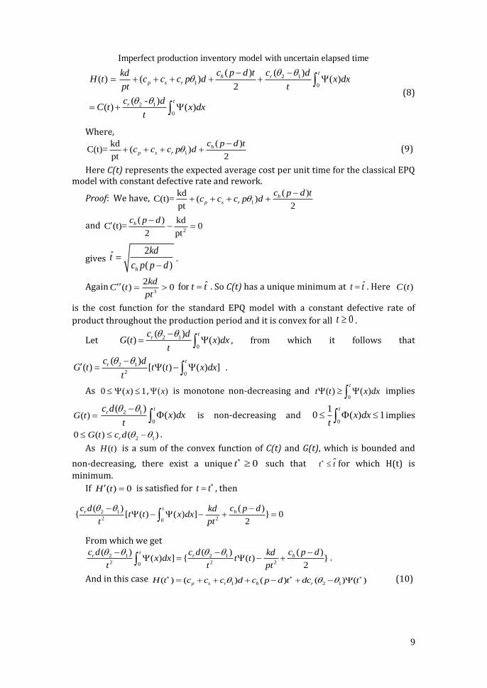
Imperfect production inventory model with uncertain elapsed time
9
2 1
10
2 1
0
( ) ( )( ) ( ) ( )
2
( - )( ) ( )
th r
p s r
tr
c p d t c dkdH t c c c p d x dx
pt t
c dC t x dx
t
(8)
Where,
1
( )kdC(t)= ( )
pt 2
h
p s r
c p d tc c c p d
(9)
Here C(t) represents the expected average cost per unit time for the classical EPQ model with constant defective rate and rework.
Proof: We have, 1
( )kdC(t)= ( )
pt 2
h
p s r
c p d tc c c p d
and 2
( ) kdC (t)= 0
2 pt
hc p d
gives 2
ˆ( )h
kdt
c p p d
.
Again3
2( ) 0
kdC t
pt ˆfor t t . So C(t) has a unique minimum at ˆ t t . Here ( )C t
is the cost function for the standard EPQ model with a constant defective rate of
product throughout the production period and it is convex for all 0t .
Let 2 1
0
( ) ( ) ( )
trc d
G t x dxt
, from which it follows that
2 1
2 0
( )( ) [ ( ) ( ) ]
trc d
G t t t x dxt
.
As 0 ( ) 1x , ( )x is monotone non-decreasing and 0
( ) ( )t
t t x dx implies
( )G t 2 1
0
( )( )
trc d
x dxt
is non-decreasing and
0
10 ( ) 1
t
x dxt
implies
2 10 ( ) ( )rG t c d .
As ( )H t is a sum of the convex function of C(t) and G(t), which is bounded and
non-decreasing, there exist a unique 0t such that t t for which H(t) is
minimum.
If ( ) 0H t is satisfied for t t , then
2 1
2 20
( )( ){ [ ( ) ( ) ] } 0
2
thr
c p dc d kdt t x dx
t pt
From which we get
2 1 2 1
2 2 20
( )( ) ( )( ) ] { ( ) }
2
thr r
c p dc d c d kdx dx t t
t t pt
.
And in this case 1 2 1( ) ( ) ( ) ( ) ( )p s r h rH t c c c d c p d t dc t (10)

Ghosh and Dey/Decis. Mak. Appl. Manag. Eng. 3 (2) (2020) 1-18
10
5. Solution
We cannot find out closed form solution of the optimum production run from the above objective function. Using the Search procedure along with the bisection method and bound of the optimum production time, a search procedure is
appliedtofind out t such that 2
( ) ( ) 0H t t F t , which gives2
r 2 10
( - )( ) t +c d( - )[ ( ) ( ) ]
2
thc p d kd
F t t t x dxp
(11)
5.1 Algorithm of the Search Procedure
Step 1: Set 0Lt and
2
( )U
h
kdt
c p p d
Where ( ) 0LF t and ( ) 0UF t , implies the existence of a value t for which( ) 0F t .
Step 2: Compute 2
L Uo
t tt
and the value of 0( )F t .
Step 3: If ( )oF t , where( 0, error tolerance).Control goes to step 5 otherwise goes to next step.
Step 4: If ( ) 0oF t , set U ot t , otherwise ( ) 0oF t , set L ot t , go to step 2.
Select the value of ot as optimum value t
. Step5. Terminate the search procedure.
6. Numerical Example
The numerical examples are given for illustrative and verification of the real world problem.
Case 1: Linear Uncertain Distribution
Consider the uncertain variable as linear with support ( , )a b , where a=2.5 and
b=10.0 and other parameters are K = 2000, 1 0.10, 2 0.20, hc 5.0, d = 50, p =
75, pc 50.0, sc 5.0., rc = 10.0.
By the search procedure, the optimum production time is t = 4.53537 and corresponding optimum cost = 3380.49.

Imperfect production inventory model with uncertain elapsed time
11
Figure 1. Expected average cost function is convex with respect to
production time
Table 1: Expected optimum production time and expected optimum cost/unit time with respect to the different change of the parameter.
Parameter
Change in
Parameter
Optimum Productio
n Time
Optimum Expected Average
Cost/Unit Time
Parameter
Change in
Parameter
Optimum Productio
n Time
Optimum Expected Average
Cost/Unit Time
P
-20% -10%
0% +10% +20%
7.71744 5.64864 4.53537 3.81795 3.30973
3220.65 3315.25 3380.49 3429.20 3467.34
1
-20% -10%
0% +10% +20%
4.51952 4.52741 4.53537 4.54340 4.55750
3371.10 3375.79 3380.49 3385.19 3389.88
D
-20% -10%
0% +10% +20%
3.46624 3.95285 4.53537 5.26842 6.25753
2851.74 3121.64 3380.49 3627.14 3859.37
2
-20% -10%
0% +10% +20%
4.56789 4.55150 4.53537 4.51952 4.50393
3379.36 3379.88 3380.49 3381.10 3381.69
K
-20% -10%
0% +10% +20%
4.06436 4.30631 4.53537 4.75341 4.96138
3318.47 3350.33 3380.49 3409.20 3436.63

Ghosh and Dey/Decis. Mak. Appl. Manag. Eng. 3 (2) (2020) 1-18
12
Figure 2. Production time with respect to the percentage change of the
different parameter
Figure 3. Optimum expected average cost/unit time with respect to the
percentage change of the different parameter.
Case 2: Zigzag Uncertain Distribution Consider the uncertain variable as zigzag Z(a, b, c) with support ( , )a c , where a =
5.0 and b = 8.0 and c=10.0 and other parameters are K = 2000, 1 0.1,
2 0.20,
hc 2.0, d=50,p=75, pc 25.0,
sc 2.0,rc = 5.0.
0
1
2
3
4
5
6
7
8
9
-30% -20% -10% 0% 10% 20% 30%
Op
tim
um
Pro
du
ctio
n T
ime
Change in Parameter
Production rate
Demand rate
Setup cost
Rate of nonconforming items in'In-control-state'
Rate of nonconforming items in'Out-of control- state'
0
500
1000
1500
2000
2500
3000
3500
4000
4500
-30% -20% -10% 0% 10% 20% 30%
Op
tim
um
To
tal c
ost
/U
nit
Tim
e
Change in Parameter
Production rate
Demand rate
Setup cost
Rate of nonconforming items in'In-control-state'
Rate of nonconforming items in'Out-of control- state'

Imperfect production inventory model with uncertain elapsed time
13
By the search procedure, the optimum production time is t = 4.55557 and
corresponding optimum cost = 3379.72.
Figure 4. Expected cost function is convex with respect to production time
Table 2. Expected optimum production time and expected optimum
cost/unit time with respect to the different change of the parameter
Parameter
Change in Parameter
Optimum
Production
Time
Optimum Expected Average
Cost/Unit Time
Paramete
r
Change in Para
meter
Optimum
Production
Time
Optimum Expected Average
Cost/Unit Time
p
-20% -10%
0% 10% 20%
7.82140 5.68945 4.55557 3.82879 3.31550
3217.68 3313.77 3379.72 3428.82 3467.18
1
-20% -10%
0% 10% 20%
4.54340 4.54947 4.55557 4.56171 4.56789
3370.19 3374.96 3379.72 3384.49 3389.26
d
-20% -10%
0% 10% 20%
3.47242 3.96434 4.55557 5.30377 6.32211
2851.56 3121.24 3379.72 3625.80 3857.09
2
-20% -10%
0% 10% 20%
4.58037 4.56789 4.55557 4.54340 4.53139
3378.79 3379.26 3379.72 3380.19 3380.64
k
-20% -10%
0% 10% 20%
4.08052 4.32457 4.55557 4.77540 4.98556
3317.97 3349.69 3379.72 3408.30 3435.62

Ghosh and Dey/Decis. Mak. Appl. Manag. Eng. 3 (2) (2020) 1-18
14
Figure 5. Production time with respect to the percentage change of
different parameters
Figure 6. Optimum cost/unit time with respect tothe percentage
change of different parameters.
7. Sensitivity Analysis
Since the shifting time point from in–control state to out-of-control state is uncertain variable in between beginning and end of the production run and it
0
1
2
3
4
5
6
7
8
9
-30% -20% -10% 0% 10% 20% 30%
Exp
ect
ed
op
tim
um
pro
du
ctio
n t
ime
Change in Parameter
Production rate (p)
Demand rate(d)
Setup Cost (k)
Rate of defective items in 'in-control state'
Rate of defective items in 'out-of-control state'
0
500
1000
1500
2000
2500
3000
3500
4000
4500
-30% -20% -10% 0% 10% 20% 30%Exp
ect
ed
op
tim
um
pro
du
ctio
n t
ime
Change in Parameter
Production rate (p)
Demand rate(d)
Setup Cost (k)
Rate of defective items in 'in-control state'
Rate of defective items in 'out-of-control state'
Imperfect production inventory model with uncertain elapsed time
15
depends on support set of uncertainty distribution, so, the optimum production time and optimum cost per unit time depending on that.
From Table-1, Figure-2 and Table-2, Figure-5, for both the cases, it is observed that optimum production time is decreased with increase of production rate and rate of reworkable defective items in ‘out-of-control’ state and it increases with the increase of other parameter demand rate, setup cost and rate of reworkable defective items in ‘in-control’ state. Similarly from Table-1, Figure-3 and Table-2, Figure-6, for both the cases, it follows that optimum cost increases with the increases of all parameters.
Optimum production time is sensitive to the change of parameters production rate (p) and demand rate (d) and optimum cost per unit time is sensitive to the change of parameter demand rate (d). Optimum production time is moderately sensitive with the change of a parameter (p), slightly sensitive to the change of a parameter (d) and insensitive to the change of all other parameters. In the same way, the optimum cost/per unit time is slightly sensitive to the changes of the parameter (d) and insensitive to all other parameters.
8. Conclusion
In this article, we have discussed an imperfect production inventory model in an uncertain environment. It is assumed that an imperfect production process has two states ‘in-control’ state and ‘out-of-control’ state. Here we also assumed that the elapsed time of the production process follow uncertain shift distribution, which is an uncertain variable follows an uncertainty distribution. The basic difference from the earlier research article is that our model is on the study of uncertain phenomena while the stochastic is about the study of stochastic phenomena. For the lack of historical data, the shifting of the production process is quantified by domain experts’ belief degree and by the principle of least square, the manager should follow a particular uncertainty distribution. The optimum production time and optimum cost depend on the type of uncertainty distribution along with the support set of that. Two case examples justify the numerical verification of theorem and propositions in this proposed model on linear and zigzag uncertainty distribution with the same support. It follows that the expected optimum cost is near about approximately the same for both the uncertainty distribution, though optimum production time is slightly different. Finally, for illustrating the procedure, an algorithm is designed to find out the optimum goal.
Inthe future, we would like to extend our modelfor the imperfect production process with random uncertain circumstances. Moreover, the possible extension of different variants of imperfect production inventory problem like demand variability and trade credit policy to uncertain single/multi-objective models will also be the area of our research interest.
Author Contributions: Each author has participated and contributed sufficiently to take public responsibility for appropriate portions of the content.
Funding: This research received no external funding.
Conflicts of Interest: The authors declare no conflicts of interest.

Ghosh and Dey/Decis. Mak. Appl. Manag. Eng. 3 (2) (2020) 1-18
16
References
Chen, C. K., & Lo, C. C. (2006). Optimal production run length for products sold with warranty in an imperfect production system with allowable shortages. Mathematical and Computer Modelling, 44, 319-331.
Chen, S. H., Wang, S. T., & Chang S. M. (2005). Optimization of fuzzy production inventory model with repairable defective products under crisp and fuzzy production quantity. International Journal of Operations Research, 2(2), 31-37.
Chen, L., Peng, J., Liu, Z., & Zaho, R. (2016). Pricing and effort decisions for a supply chain with uncertain information. International Journal of Production Research, 55(1), 264-284.
Chiu, S. W., Wang, S. L., & Chiu, Y. S. P. (2007). Determining the optimal run time for EPQ model with scrap, rework, stochastic breakdowns. European Journal of Operational Research, 180, 664-676.
Chiu, Y. S. P., Chen, K. K., Cheng, F. T., & Wu, M. F. (2010). Optimization of the finite production rate with scrap, rework and stochastic machine breakdown. Computers and Mathematics with Applications, 59, 919-932.
Gao Y., & Kar S., (2017). Uncertain solid transportation problem with product blending. International Journal of Fuzzy Systems, 19(6), 1916-1926.
Hiriga, M., & Ben Daya, M. (1998). The economic manufacturing lot-sizing problem with imperfect production process: Bounds and optimal solutions. Naval Research Logistics, 45, 423-432.
Hu, F., & Zong, Q. (2009). Optimal production run time for a deteriorating production system under an extended inspection policy. European Journal of Operational Research, 196, 979-986.
Hussain, A. Z. M. O., & Murthy, D. N. P. (2003). Warranty and Optimal Reliability Improvement through Product Development. Mathematical and Computer Modelling, 38, 1211-1217.
Jiang, Y., Yan, H., & Zhu, Y. (2016). Optimal Control Problem for uncertain linear systems with multiple input delays. Journal of Uncertainty Analysis and Applications, 4, 1-15.
Kar, M. B., Majumder, S., Kar, S., & Pal, T. (2017). Cross-entropy based multi-objective uncertain portfolio selection problem. Journal of Intelligent & Fuzzy Systems, 32(6), 4467-4483.
Ke, H., Li, Y., & Huang ,H. (2015). Uncertain pricing decision problem in closed-loop supply chain with risk-averse retailer. Journal of Uncertainty Analysis and Application, 3, 1-14.
Ke, H., & Liu, B. (2010). Fuzzy Project Scheduling problems and its hybrid intelligent Algorithm. Applied Mathematical Modeling, 34(2), 301-308.
Khouja, M., & Meherez, A (1994). An economic production lot size model with imperfect quality and variable production rate. Journal of the Operational Research Society, 45, 1405-1417.

Imperfect production inventory model with uncertain elapsed time
17
Liu, B. (2012). Why is there a need for uncertainty theory?. Journal of Uncertainty Systems, 6(1), 3-10.
Liu, B. (2015). Uncertainty theory: A branch of Mathematics for Modeling Human uncertainty. (4th ed.). Berlin: Springer-Verlag.
Liu, B. (2016). Uncertainty theory: A branch of Mathematics for Modeling Human uncertainty. In Liu, B Uncertainty Theory (pp. 1-79). Berlin: Springer-Verlag.
Liu, B. (2009). Theory and Practice of Uncertain Programming. (2nd ed.). Berlin: Springer-Verlag.
Liu, Y., & Ha, M. (2010). Expected value of function of uncertain variables. Journal of Uncertain Systems, 4(3), 181-186.
Liu,Y., Li, X., & Xiong, C. (2015). Reliability analysis of unrepairable systems with uncertain lifetimes. International Journal of Security and its Application, 9(12), 289-298.
Majumder, S., Kar, S., & Pal, T. (2018). Mean-Entropy Model of Uncertain Portfolio Selection Problem. In: JK Mandal, S, Mukhopadhyay, P, Dutta (Eds.), Multi-Objective Optimization: Evolutionary to Hybrid Framework. (pp. 25-54). Singapore: Spinger.
Majumder, S., Kundu, P., Kar, S., Pal, T. (2018). Uncertain multi-objective multi-item fixed charge solid transportation problem with budget constraint. In Majumder, S., Kundu, P., Kar, S., Pal, T (Eds.), Soft Computing (pp.3279-3301). Berlin: Springer.
Qin, Z., & Kar, S. (2013). Single-period inventory problem under uncertain environment. Applied Mathematics and Computation, 219, 9630-9638.
Qin Z., Kar, S., & Zheng, H. (2016). Uncertain portfolio adjusting model using semiabsolute deviation. Soft Computing, 20(2), 717-725.
Rosenbaltt, M. J., & Lee, H. L. (1986). Economic production cycles with imperfect production process. IIE Transactions, 17, 48-54.
Sana, S. S. (2010). An economic production lot size model in an imperfect production system. European Journal of Operational Research, 201, 158-170.
Sana, S. S. (2010). A production-inventory model in an imperfect production process. European Journal of Operational Research, 200, 451-64.
Wang, D., Qin Z., & Kar, S. (2015). A novel single period inventory problem with uncertain random demand and its application. Applied Mathematics and Computation, 269, 133-145.
Wang, X., & Tang, W. (2009). Optimal production run length in deteriorating production process with fuzzy elapsed time. Computer and Industrial Engineering, 56, 1627-1632.
Widyadana, G. A., & Wee, H. M. (2011). Optimal deteriorating items production inventory models with random machine breakdown and stochastic repair time. Applied Mathematical Modelling, 35(7), 3495-3508.
Yeh, R. H., Ho, W. T., & Tseng, S. T. (2000). Optimal production run length for products sold with warranty. European Journal of Operational Research, 120, 575-582.

Ghosh and Dey/Decis. Mak. Appl. Manag. Eng. 3 (2) (2020) 1-18
18
Yeh, R. H., Chen, M. Y., & Lin, C. Y. (2007). Optimal periodic replacement policy for repairable products under free-repair warranty. European Journal of Operational Research, 176, 1678-1686.
Yeo, W. M., & Yuan, XueMing. (2009). Optimal warranty policies for systems with imperfect repair. European Journal of Operational Research, 199, 187-197.
Yun, Won Young., Murthy, D. N. P. & Jack, N. (2008). Warranty servicing with imperfect repair. International Journal of Production Economics, 111, 159-169.
Zhou, C., Tang, W., & Zhao, R. (2014). An uncertain search model for recruitment problem with enterprise performance. Journal of Intelligent Manufacturing, 28(3), 695-704.
© 2018 by the authors. Submitted for possible open access publication under
the terms and conditions of the Creative Commons Attribution (CC BY) license
(http://creativecommons.org/licenses/by/4.0/).