implementation and integration of an experimental vehicle

Implementation and Integration of anExperimental Vehicle Sensor Setup forAutomated ParkingErtüchtigung und Aufbau eines Versuchsträger-Sensor-Setups für automatisiertes ParkenBearbeiter: Alberto Linares | 2288833Betreuer: Philipp Rosenberger, M.Sc.

Alberto LinaresMatrikelnummer: 2288833Studiengang: Allgemeiner Maschinenbau

Bachelor-Thesis Nr. 1318-18Thema: Implementation and Integration of an Experimental Vehicle Sensor Setup for Automated Parking

Eingereicht: September 17, 2018

Technische Universität DarmstadtFachgebiet FahrzeugtechnikProf. Dr. rer. nat. Hermann WinnerOtto-Berndt-Straße 264287 Darmstadt

Erklärung zur Bachelor-Thesis

Hiermit versichere ich, Alberto Linares, die vorliegende Bachelor-Thesis gemäß § 22 Abs.7 APB der TU Darmstadt ohne Hilfe Dritter nur mit den angegebenen Quellen undHilfsmitteln angefertigt zu haben. Alle Stellen, die aus Quellen entnommen wurden, sindals solche kenntlich gemacht worden. Diese Arbeit hat in gleicher oder ähnlicher Formnoch keiner Prüfungsbehörde vorgelegen.Mir ist bekannt, dass im Falle eines Plagiats (§38 Abs.2 APB) ein Täuschungsversuchvorliegt, der dazu führt, dass die Arbeit mit 5,0 bewertet und damit ein Prüfungsversuchverbraucht wird. Abschlussarbeiten dürfen nur einmal wiederholt werden.Bei der abgegebenen Thesis stimmen die schriftliche und die zur Archivierung eingereichteelektronische Fassung gemäß § 23 Abs. 7 APB überein.

Darmstadt, den 4.2.2016

(Alberto Linares)

Abstract

This thesis has been realized for the automotive engineering department of the TU-Darmstadt University.This department is currently carrying out research in the field of sensor modeling to support autonomousdriving.

During this thesis the main objective is the rear sensors Bosch parkpilot URF7 implementation andintegration, using the methodology described by the thesis1. Besides, part of the results obtained havebeen used for the modeling of ultrasonic sensors for valet parking use cases.

The thesis is divided in different stages. First of all, a documented bibliographic search will be carriedout on the ultrasonic sensors general operation and the different most important technical specificationsof an ultrasonic sensor in the field of the automotive industry as well. Among them are: the field of view,detectable objects distance ranges and accuracy of the measurement. Once the necessary information forthe thesis has been obtained, the Bosch Parkpilot URF7 has been used and the different tests previouslydescribed in the methodology research have been elaborated. Besides, imparting of the initial method-ology extra tests have been made based on the calculation of the distance between sensor and object inreal time. It should be noted that all these tests have been run without the sensor setup installation inthe car. In contrast, the position and orientation of the sensors has been fixed as in the institutes testvehicle, Honda Accord, thanks to a movable platform.

Once the system has been installed and powered with an external power supply, the basic functionalityas an user level has been checked, in other words, the system calibration and the operating mode. Toget a better understanding of the operation, the board that controls the Bosch sensor setup has beenexamined. The actual functioning of the existing hardware could not be found successfully due to thelack of information from the manufacturers. However, it is known the existence of a communication be-tween sensors and the control unit, so that, with the realization of different tests and observing its signalwith a DAQ, the signals can be read an processed. Once the operation of this Bus has been checked, thedifferent experiments are performed to determine some technical specifications of the sensors: the fieldof vision (both of a sensor and of the entire sensor setup), the distance range in which a object can bedetected, the operation of the cross echo and the accuracy in the measurement.

Finally, with an Arduino UNO the signal of the communication bus has been processed to obtain thedistance to an object as accurate as possible in real time. In addition, the sensitivity of the resultsobtained with the Arduino will also be determined.

1 Fu, J. et al.: Setup for ultrasonic models validation (2017)

Contents

1 Introduction1.1 Motivation . . . . . . . . . . . . . . . . . . . . . . . . . . . . . . . . . . . . . . . . . . . . . . . . .1.2 Methodology . . . . . . . . . . . . . . . . . . . . . . . . . . . . . . . . . . . . . . . . . . . . . . . .1.3 Concretion of Assignment . . . . . . . . . . . . . . . . . . . . . . . . . . . . . . . . . . . . . . . .

2 Ultrasonic Sensors2.1 Conversion Principles . . . . . . . . . . . . . . . . . . . . . . . . . . . . . . . . . . . . . . . . . . .

2.1.1 Piezoelectric Effect . . . . . . . . . . . . . . . . . . . . . . . . . . . . . . . . . . . . . . .2.1.2 Piezoelectric Material . . . . . . . . . . . . . . . . . . . . . . . . . . . . . . . . . . . . . .

2.2 Ultrasonic Transducer . . . . . . . . . . . . . . . . . . . . . . . . . . . . . . . . . . . . . . . . . .2.2.1 Active Element . . . . . . . . . . . . . . . . . . . . . . . . . . . . . . . . . . . . . . . . . .2.2.2 Backing and Wear Plate . . . . . . . . . . . . . . . . . . . . . . . . . . . . . . . . . . . .2.2.3 Equivalent Circuit . . . . . . . . . . . . . . . . . . . . . . . . . . . . . . . . . . . . . . . .

2.3 Distance Measurements . . . . . . . . . . . . . . . . . . . . . . . . . . . . . . . . . . . . . . . . .2.3.1 Distances Between Pulses . . . . . . . . . . . . . . . . . . . . . . . . . . . . . . . . . . .2.3.2 Object Localization and Trilateration . . . . . . . . . . . . . . . . . . . . . . . . . . . .

3 Bosch Parkpilot URF73.1 Technical Specifications . . . . . . . . . . . . . . . . . . . . . . . . . . . . . . . . . . . . . . . . .3.2 System Calibration . . . . . . . . . . . . . . . . . . . . . . . . . . . . . . . . . . . . . . . . . . . .3.3 Bosch Parkpilot URF7 Operation . . . . . . . . . . . . . . . . . . . . . . . . . . . . . . . . . . .

4 Bosch Parkpilot URF7 Tests4.1 Hardware and Software . . . . . . . . . . . . . . . . . . . . . . . . . . . . . . . . . . . . . . . . .

4.1.1 Power Supply . . . . . . . . . . . . . . . . . . . . . . . . . . . . . . . . . . . . . . . . . . .4.1.2 National Instrument DAQ and Labview . . . . . . . . . . . . . . . . . . . . . . . . . . .4.1.3 Arduino . . . . . . . . . . . . . . . . . . . . . . . . . . . . . . . . . . . . . . . . . . . . . .4.1.4 Static Tests Setup . . . . . . . . . . . . . . . . . . . . . . . . . . . . . . . . . . . . . . . .

4.2 COMM Bus Operation . . . . . . . . . . . . . . . . . . . . . . . . . . . . . . . . . . . . . . . . . .4.3 Distance Measurement Test . . . . . . . . . . . . . . . . . . . . . . . . . . . . . . . . . . . . . . .4.4 Maximum and Minimum Range Distance . . . . . . . . . . . . . . . . . . . . . . . . . . . . . .4.5 Sensor Field of View Determination . . . . . . . . . . . . . . . . . . . . . . . . . . . . . . . . . .

4.5.1 Cross Echo Operation . . . . . . . . . . . . . . . . . . . . . . . . . . . . . . . . . . . . . .4.5.2 Whole Setup Field Of View Determination . . . . . . . . . . . . . . . . . . . . . . . . .

4.6 Real Time Distance Measurement . . . . . . . . . . . . . . . . . . . . . . . . . . . . . . . . . . .4.6.1 Hardware Preparation . . . . . . . . . . . . . . . . . . . . . . . . . . . . . . . . . . . . . .4.6.2 Software Operation . . . . . . . . . . . . . . . . . . . . . . . . . . . . . . . . . . . . . . .4.6.3 Sensitivity Measurement . . . . . . . . . . . . . . . . . . . . . . . . . . . . . . . . . . . .

5 Conclusions

6 annexes

References

Version: September 17, 2018

List of Figures

1 Emitter and receiver Bosch ultrasonic sensor. . . . . . . . . . . . . . . . . . . . . . . . . . . . .2 Emitter and receiver HC-SR04 sensor. . . . . . . . . . . . . . . . . . . . . . . . . . . . . . . . .3 Vertical/Horizontal ultrasonic sensor field of view. . . . . . . . . . . . . . . . . . . . . . . . . .4 Piezoelectric effect . . . . . . . . . . . . . . . . . . . . . . . . . . . . . . . . . . . . . . . . . . . .5 Inverse piezoelectric effect . . . . . . . . . . . . . . . . . . . . . . . . . . . . . . . . . . . . . . . .6 Titanate of lead zirconate in crystalline perovskite structure. Above and below the Curie

temperature . . . . . . . . . . . . . . . . . . . . . . . . . . . . . . . . . . . . . . . . . . . . . . . .7 Different ultrasonic transducer parts . . . . . . . . . . . . . . . . . . . . . . . . . . . . . . . . .8 Transducer equivalent circuit . . . . . . . . . . . . . . . . . . . . . . . . . . . . . . . . . . . . . .9 Ultrasound wave and its envelope wave. . . . . . . . . . . . . . . . . . . . . . . . . . . . . . . .10 Trilateration obstacle distance measurement . . . . . . . . . . . . . . . . . . . . . . . . . . . .11 Bosch Parkpilot URF7. . . . . . . . . . . . . . . . . . . . . . . . . . . . . . . . . . . . . . . . . .12 LEDs distribution and sensor wiring harness . . . . . . . . . . . . . . . . . . . . . . . . . . . .13 Bosch Parkpilot URF7 operation . . . . . . . . . . . . . . . . . . . . . . . . . . . . . . . . . . .14 Final Setup for the experiments . . . . . . . . . . . . . . . . . . . . . . . . . . . . . . . . . . . .15 Experiments block diagram . . . . . . . . . . . . . . . . . . . . . . . . . . . . . . . . . . . . . . .16 Voltcracft power supply . . . . . . . . . . . . . . . . . . . . . . . . . . . . . . . . . . . . . . . . .17 NI hardware and Labview softwae implemented . . . . . . . . . . . . . . . . . . . . . . . . . .18 Arduino UNO Rev3 board . . . . . . . . . . . . . . . . . . . . . . . . . . . . . . . . . . . . . . .19 Previous static tests setup . . . . . . . . . . . . . . . . . . . . . . . . . . . . . . . . . . . . . . . .20 Layout for the setup bar. . . . . . . . . . . . . . . . . . . . . . . . . . . . . . . . . . . . . . . . .21 New setup bar . . . . . . . . . . . . . . . . . . . . . . . . . . . . . . . . . . . . . . . . . . . . . . .22 Fixing pieces for sensors . . . . . . . . . . . . . . . . . . . . . . . . . . . . . . . . . . . . . . . . .23 COMM Bus signal different pulses . . . . . . . . . . . . . . . . . . . . . . . . . . . . . . . . . .24 COMM Bus signal no object detection . . . . . . . . . . . . . . . . . . . . . . . . . . . . . . . .25 COMM Bus signal one object detection . . . . . . . . . . . . . . . . . . . . . . . . . . . . . . .26 Two objects detected in the same period . . . . . . . . . . . . . . . . . . . . . . . . . . . . . . .27 Wall test setup . . . . . . . . . . . . . . . . . . . . . . . . . . . . . . . . . . . . . . . . . . . . . . .28 Object detection probability in ten periods . . . . . . . . . . . . . . . . . . . . . . . . . . . . .29 Field of View experiment procedure . . . . . . . . . . . . . . . . . . . . . . . . . . . . . . . . . .30 Sensor position to determine both FoV . . . . . . . . . . . . . . . . . . . . . . . . . . . . . . . .31 Point objects used for the experiments . . . . . . . . . . . . . . . . . . . . . . . . . . . . . . . .32 Echo behaviour depending on the shape . . . . . . . . . . . . . . . . . . . . . . . . . . . . . . .33 Bosch sensor horizontal field of view . . . . . . . . . . . . . . . . . . . . . . . . . . . . . . . . .34 Bosch sensor vertical field of view . . . . . . . . . . . . . . . . . . . . . . . . . . . . . . . . . . .35 Cross-Echo Setup. . . . . . . . . . . . . . . . . . . . . . . . . . . . . . . . . . . . . . . . . . . . . .36 COMM Bus signal cross echo for different scenarios. . . . . . . . . . . . . . . . . . . . . . . .37 Whole system FoV metal stick . . . . . . . . . . . . . . . . . . . . . . . . . . . . . . . . . . . . .38 Whole system FoV plastic stick . . . . . . . . . . . . . . . . . . . . . . . . . . . . . . . . . . . .39 Voltage divider schematic . . . . . . . . . . . . . . . . . . . . . . . . . . . . . . . . . . . . . . . .40 Arduino connexions . . . . . . . . . . . . . . . . . . . . . . . . . . . . . . . . . . . . . . . . . . . .41 Example of a large object situation. . . . . . . . . . . . . . . . . . . . . . . . . . . . . . . . . . .42 Samples in a short distance and N=20 . . . . . . . . . . . . . . . . . . . . . . . . . . . . . . . .43 Samples in a medium distance and N=20 . . . . . . . . . . . . . . . . . . . . . . . . . . . . . .


44 Samples in a large distance and N=20 . . . . . . . . . . . . . . . . . . . . . . . . . . . . . . . .45 Samples in a short distance and N=50 . . . . . . . . . . . . . . . . . . . . . . . . . . . . . . . .46 Samples in a short distance and N=50 . . . . . . . . . . . . . . . . . . . . . . . . . . . . . . . .47 Samples in a short distance and N=50 . . . . . . . . . . . . . . . . . . . . . . . . . . . . . . . .48 Samples in a short distance and N=100 . . . . . . . . . . . . . . . . . . . . . . . . . . . . . . .49 Samples in a medium distance and N=100 . . . . . . . . . . . . . . . . . . . . . . . . . . . . .50 Samples in a large distance and N=100 . . . . . . . . . . . . . . . . . . . . . . . . . . . . . . .51 Samples in a short distance and N=200 . . . . . . . . . . . . . . . . . . . . . . . . . . . . . . .52 Samples in a medium distance and N=200 . . . . . . . . . . . . . . . . . . . . . . . . . . . . .53 Samples in a large distance and N=200 . . . . . . . . . . . . . . . . . . . . . . . . . . . . . . .54 Samples in a short distance and N=400 . . . . . . . . . . . . . . . . . . . . . . . . . . . . . . .55 Samples in a medium distance and N=400. . . . . . . . . . . . . . . . . . . . . . . . . . . . . .56 Samples in a large distance and N=400 . . . . . . . . . . . . . . . . . . . . . . . . . . . . . . .


List of Tables

1 Bosch Parkpilot URF7 tech specs. . . . . . . . . . . . . . . . . . . . . . . . . . . . . . . . . . . .2 Arduino UNO Rev3 technical specifications . . . . . . . . . . . . . . . . . . . . . . . . . . . . .3 FoV Bosch sensor measurements. . . . . . . . . . . . . . . . . . . . . . . . . . . . . . . . . . . .4 Metal stick whole FoV measurements. . . . . . . . . . . . . . . . . . . . . . . . . . . . . . . . .5 Plastic stick whole FoV measurements. . . . . . . . . . . . . . . . . . . . . . . . . . . . . . . . .6 Measured value for a short actual distance. . . . . . . . . . . . . . . . . . . . . . . . . . . . . .7 Measured value for a medium actual distance. . . . . . . . . . . . . . . . . . . . . . . . . . . .8 Measured value for a large actual distance. . . . . . . . . . . . . . . . . . . . . . . . . . . . . .9 Short distance sensitivity experiment results. . . . . . . . . . . . . . . . . . . . . . . . . . . . .10 Medium distance sensitivity experiment results. . . . . . . . . . . . . . . . . . . . . . . . . . .11 Long distance sensitivity experiment results. . . . . . . . . . . . . . . . . . . . . . . . . . . . .


1 Introduction

Nowadays there is a high interest to make cars as autonomous as possible and new technologies arehelping to achieve it. The investments for developing fully autonomous cars are increasing day by dayand did not reach their peak yet. With the responsibility of driving human beings, these cars have tobe tested absolutely carefully. However, due to the advanced technology, testing is highly costly andtime-consuming, limiting the number of testable scenarios.

Talking about parking scenarios, there are a lot of human drivers out there that can not quite handlethe parallel parking job, mainly because they lack a perspective view on the object’s surrounding them.It especially occurs in big cities with lots of cars and tight spaces for parking causing traffic tie-ups,vehicle damage. To help human drivers in such situations, Advanced Driver Assistance Systems (ADAS)have been developed. Systems which help you to drive, in this case, help you to park. ADAS warn youof the object proximity while you are parking with an acoustic signal. Others are more sophisticated anduse cameras showing the human driver a real time picture of the car’s surrounding. Latest tech systemsare even able to park the car autonomously.

1.1 Motivation

The motivation of this thesis is presented as a contribution for the before mentioned problems, sincetogether with a master thesis2 that is running in parallel, the final objective is to validate a ultrasonicsensor model in valet parking use cases. Besides, it is colaborated for the ENABLE-S3 project inthe development of simulation environments with the purpose of implementing an autonomous parkingsystem. Therefore, all those problems that the human driver has when is parking will disappear. Besides,being able to recreate with the simulations environment infinite situations in a more efficient, cheap andfast way with the purpose of improving and checking all these systems, seeing that real environmenttests are too expensive3.

1.2 Methodology

This thesis has had a duration of 5 months in which differents methods has been followed to arrive at anobjective with final results and conclusions. Note that for the collection of these results has been neededa power supply, which simulated the reverse gear feeding thus the setup. In addition, a DAQ connectedto a computer, which had a Labview script implemented for the acquisition of data from the sensor setup,was needed. Remark that the chosen software was Labview due to its easy implementation with the DAQand because it has implemented a graphical interficie that shows the information in a very visual way. Toknow the operation of the communication between sensor-ECU a deductive method was applied, sincefrom the basic general knowledge of the ultrasound sensors the operation of this was deduced. Observingthe signal while a object was placed at different distances and positions or even removing the object.Then, to determine the different technical specifications, a method of experimentation has been applied,in other words, some differents experiments were carried out to determine them. Finally, a method ofcollecting data and sampling these in real time will be realized with a microprocessor. In this case an

2 Fu, J.: Ultrasonic sensor model (2018)3 Kishonti, L.: Real and simulated tests (2017)


Arduino since the university had one and Arduino is enough fast and valid for the application to beimplemented.

1.3 Concretion of Assignment

The concrete assigment of this thesis is to build up a sensor setup to collect real data which will then beused to validate sensor models of ultrasonic sensors in valet parking use cases. In this thesis, URF7 Boschautoparking pilot are the sensors studied. The first part of the thesis consists of analyzing and knowingthe operation of the setup at a basic use level, apart from learning about the operation of ultrasoundsensors at a general level. The second part, consists of studying the setup at a more technical level. Itincludes to find out the operation of the communication signal to analyze the communication betweensensors and controller. With the purpose of getting real data, different experiments were performed suchas obtaining the exact distance between object and sensor, determining maximum and minimum rangethat a sensor is able to detect an object and determining the field of view of both sensor and whole setup.Furthermore, a method was developed for starting, collecting, saving and reproducing measurement datain real time of the ultrasonic sensors. Finally, all the information and results obtained in the differentexperiments were documented.


2 Ultrasonic Sensors

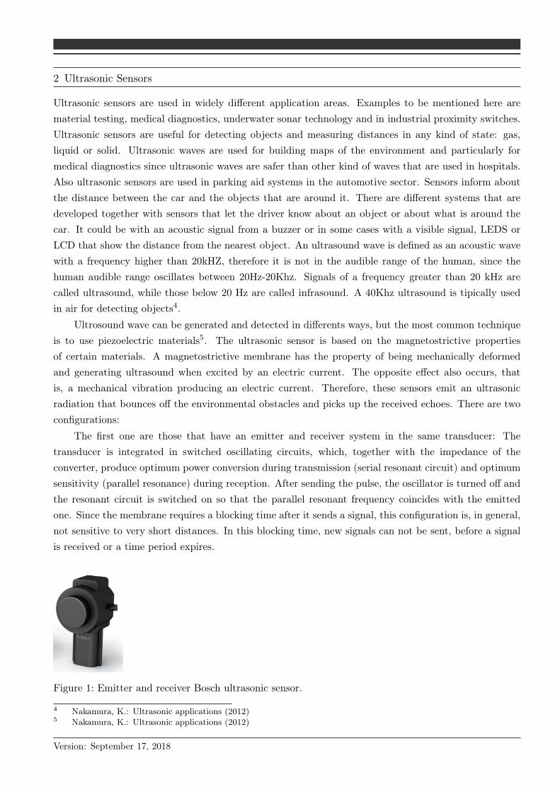
Ultrasonic sensors are used in widely different application areas. Examples to be mentioned here arematerial testing, medical diagnostics, underwater sonar technology and in industrial proximity switches.Ultrasonic sensors are useful for detecting objects and measuring distances in any kind of state: gas,liquid or solid. Ultrasonic waves are used for building maps of the environment and particularly formedical diagnostics since ultrasonic waves are safer than other kind of waves that are used in hospitals.Also ultrasonic sensors are used in parking aid systems in the automotive sector. Sensors inform aboutthe distance between the car and the objects that are around it. There are different systems that aredeveloped together with sensors that let the driver know about an object or about what is around thecar. It could be with an acoustic signal from a buzzer or in some cases with a visible signal, LEDS orLCD that show the distance from the nearest object. An ultrasound wave is defined as an acoustic wavewith a frequency higher than 20kHZ, therefore it is not in the audible range of the human, since thehuman audible range oscillates between 20Hz-20Khz. Signals of a frequency greater than 20 kHz arecalled ultrasound, while those below 20 Hz are called infrasound. A 40Khz ultrasound is tipically usedin air for detecting objects4.

Ultrosound wave can be generated and detected in differents ways, but the most common techniqueis to use piezoelectric materials5. The ultrasonic sensor is based on the magnetostrictive propertiesof certain materials. A magnetostrictive membrane has the property of being mechanically deformedand generating ultrasound when excited by an electric current. The opposite effect also occurs, thatis, a mechanical vibration producing an electric current. Therefore, these sensors emit an ultrasonicradiation that bounces off the environmental obstacles and picks up the received echoes. There are twoconfigurations:

The first one are those that have an emitter and receiver system in the same transducer: Thetransducer is integrated in switched oscillating circuits, which, together with the impedance of theconverter, produce optimum power conversion during transmission (serial resonant circuit) and optimumsensitivity (parallel resonance) during reception. After sending the pulse, the oscillator is turned off andthe resonant circuit is switched on so that the parallel resonant frequency coincides with the emittedone. Since the membrane requires a blocking time after it sends a signal, this configuration is, in general,not sensitive to very short distances. In this blocking time, new signals can not be sent, before a signalis received or a time period expires.

Figure 1: Emitter and receiver Bosch ultrasonic sensor.

4 Nakamura, K.: Ultrasonic applications (2012)5 Nakamura, K.: Ultrasonic applications (2012)


On the other hand, those that have a separate emitter and receiver system: Ultrasonic waves aregenerated with one of the membranes, while the other membrane is used to receive the ultrasonic waves.In this configuration, the receiving membrane is prepared to listen from the same instant in which thewaves have just been emitted and therefore it is usually appropriate to measure very short distances thatthe configuration of a common emitter and receiver can not reach.

Figure 2: Emitter and receiver HC-SR04 sensor.

In both configurations, sensors can be affected by the cross-talking phenomenon. What it means isthat the echo signal is received by another sensor or the same sensor from a previous shot if the waitingtimes between shots are not adequate.

Ultrasonic sensors have two sensitive detection angles, the horizontal and the vertical angles. Forthe automotive sector, it is interesting that the horizontal detection range is wide, while it is best if thevertical one is not wide, to avoid reflections with the ground 6. There are also other secondary lobes inwhich the sensor is also somewhat sensitive, but not too much.

Figure 3: Vertical/Horizontal ultrasonic sensor field of view7.

Sensors have a maximum detection distance, which depends to a large extent on the frequency ofthe ultrasonic wave, the sensitivity of the electronics and the membrane, and of course the transmissionmedium; if it is air, the wave degrades rapidly compared to aquatic environments. For the case ofultrasound in the air sensors can measure maximum distances of 3 or 4 meters.

Depending on the surface on which the signal bounces, rough or on an edge, it may be that theobject is not detected, since the bounced signal would not be detected by the receiver. Normally, crystalsand mirrors are theoretically detected, but their thickness may not be detected correctly. Colors do notaffect this sensor.6 Winner, H.: Handbook of Driver Assistance Systems (2014)7 Fu, J. et al.: Setup for ultrasonic models validation (2017)


2.1 Conversion Principles

2.1.1 Piezoelectric Effect

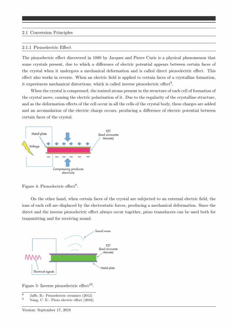
The piezoelectric effect discovered in 1880 by Jacques and Pierre Curie is a physical phenomenon thatsome crystals present, due to which a difference of electric potential appears between certain faces ofthe crystal when it undergoes a mechanical deformation and is called direct piezoelectric effect. Thiseffect also works in reverse. When an electric field is applied to certain faces of a crystalline formation,it experiences mechanical distortions, which is called inverse piezoelectric effect8.

When the crystal is compressed, the ionized atoms present in the structure of each cell of formation ofthe crystal move, causing the electric polarization of it. Due to the regularity of the crystalline structure,and as the deformation effects of the cell occur in all the cells of the crystal body, these charges are addedand an accumulation of the electric charge occurs, producing a difference of electric potential betweencertain faces of the crystal.

Figure 4: Piezoelectric effect9.

On the other hand, when certain faces of the crystal are subjected to an external electric field, theions of each cell are displaced by the electrostatic forces, producing a mechanical deformation. Since thedirect and the inverse piezoelectric effect always occur together, piezo transducers can be used both fortransmitting and for receiving sound.

Figure 5: Inverse piezoelectric effect10.

8 Jaffe, B.: Piezoelectric ceramics (2012)9 Yang, C. E.: Piezo electric effect (2016)


2.1.2 Piezoelectric Material

The piezoelectric effect can only occur in non-conductive materials. In addition, all non-conductiveferroelectric materials or permanent electric dipole materials are also piezoelectric. Only quartz is usedtoday commercially. The most important piezoelectric crystals from the practical point of view areobtained artificially.

Piezoelectric monocrystalline materials are still being developed, but the most widely used piezoelec-tric materials are polycrystalline ceramic materials and polymers. These materials present piezoelectriccharacter after having been subjected to an artificial polarization. The most commonly used piezoelectricceramic is called lead zirconate titanate (PZT)11.

Piezoceramic materials have the property of being rigid and ductile, so they are good candidatesfor use as actuators, due to their large modulus of elasticity, which facilitates the mechanical couplingwith the structure. In contrast, piezo-polymers are better prepared to act as sensors because they addminimal rigidity to the structure and are also easy to process. The most common way to use them is ascontact sensors and acoustic transducers in the form of a thin sheet 12.

Dissymmetry in the distribution of positive and negative electrical charges sets in within the latticeof a cell below the so-called Curie temperature. This results in a permanent electric dipole moment ofthe single cell (Figure 6). The ferroelectricity is given from the development of domains with uniformelectrical polarization that are aligned by the polarity, i.e., by a strong electrical constant field appliedfor a short time. The polarity is associated with a change in the length of the ceramic

The work in the field of lead-free piezoelectric ceramics has been intensive as part of the efforts notto use lead in the vehicle wherever possible. There is however no alternative to using today’s ceramicsthat can be expected in the short term from this research.

Figure 6: Titanate of lead zirconate in crystalline perovskite structure. Above and below the Curietemperature13.

10 Yang, C. E.: Piezo electric effect (2016)11 Nakamura, K.: Ultrasonic applications (2012)12 Jaffe, B.: Piezoelectric ceramics (2012)13 Winner, H.: Handbook of Driver Assistance Systems (2014)


2.2 Ultrasonic Transducer

A transducer is a device that can convert one form of energy into another, in the case of an ultrasoundtransducer converts electrical energy into mechanical waveform and mechanical into electrical energy, itis for this reason that most ultrasound transducers can be used to pulse echo application.

For ultrasound-based parking assist systems, a working frequency in the range of 40 to 50 kHz hasproven to be the best compromise between competitive demands for good system performance (sensitivity,range, etc.) on the one hand , and high robustness against strange sounds on the other hand. Higherfrequencies lead to lower echo amplitudes due to higher acoustic attenuation in the air, while for lowerfrequencies the proportion of noise sources in the vehicle environment increases more and more14.

Figure 7 shows a general scheme of an ultrasound transducer in which the main parts of it canbe observed, which are the following: Active or piezoelectric element, Backing and Wear Plate. Theimportance and functioning of them are explained below.

Figure 7: Different ultrasonic transducer parts15.

2.2.1 Active Element

The active element or piezoelectric element is responsible for carrying out the electromechanical conver-sion previously expected, which is electrically connected to the outside through welded contacts in theelectrodes that cover the piezoelectric element. Along with this element, other non-active elements arefound that determine the temporary characteristics of emission and / or reception. These elements arethe so-called "Backing" and wear plate. Among the different types of piezoelectric elements, piezoelec-tric ceramics (PZT: lead zirconate titanate) are the most commonly used due to their high conversionefficiency16.

2.2.2 Backing and Wear Plate

These passive mechanical systems named in section 2.2 have as function to perform an emission asymme-try, which is understood as follows. The piezoelectric plate vibrates, emitting mechanical energy in bothdirections. The practical applications, only use the emission in only one of the faces. To this end, the14 Winner, H.: Handbook of Driver Assistance Systems (2014)15 Olympus, N.: Ultrasonic Transducers (2006)16 Rubio, C.: Ultrasonic transducer for automated sytems (2018)


countermass is placed on the back face, whose fundamental objective is to absorb the mechanical energyin that direction and stop the oscillation of the ceramic, originating a transducer with higher resolution.

The Wear plate on its part has two functions, protecting the active element and ensuring greaterenergy transfer, the latter is achieved by manufacturing it from a material with an intermediate acousticimpedance between the active element and the material on which it is expected to use the transducer17.

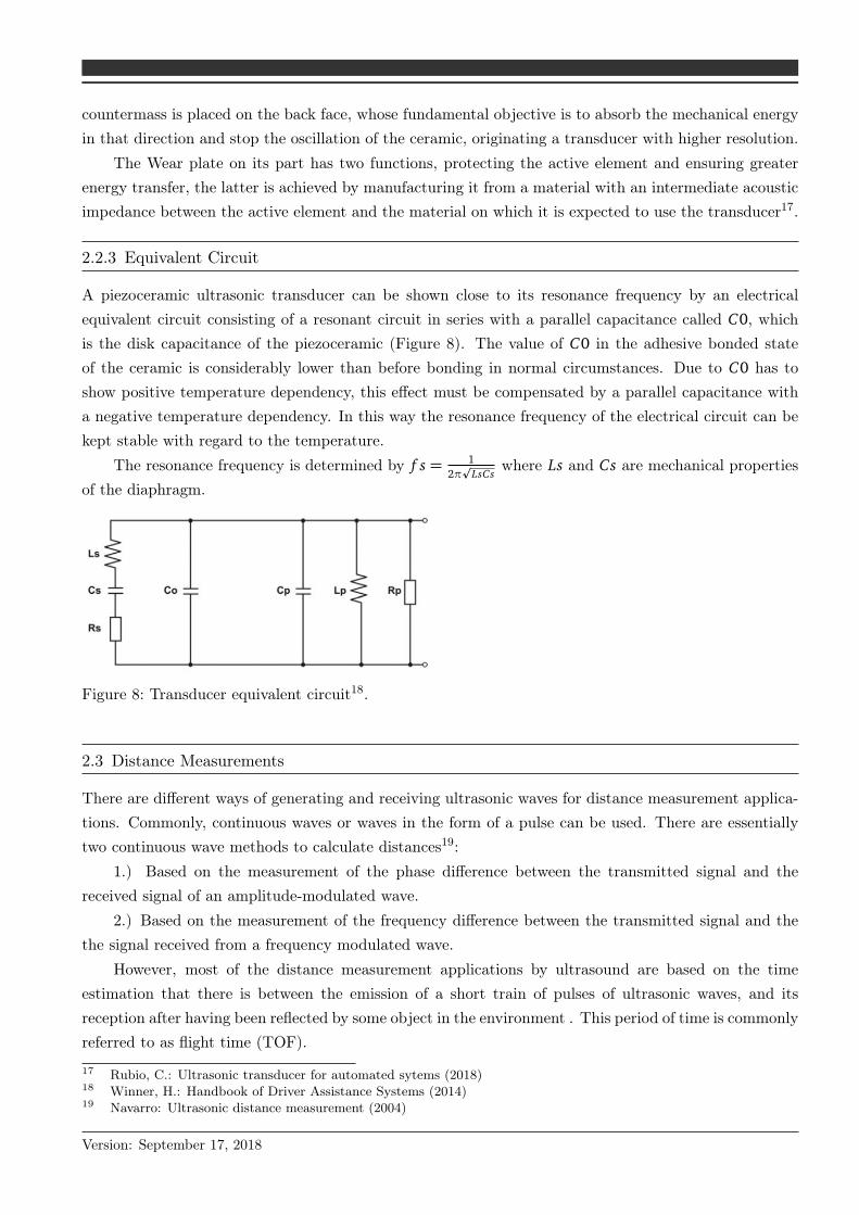
2.2.3 Equivalent Circuit

A piezoceramic ultrasonic transducer can be shown close to its resonance frequency by an electricalequivalent circuit consisting of a resonant circuit in series with a parallel capacitance called C0, whichis the disk capacitance of the piezoceramic (Figure 8). The value of C0 in the adhesive bonded stateof the ceramic is considerably lower than before bonding in normal circumstances. Due to C0 has toshow positive temperature dependency, this effect must be compensated by a parallel capacitance witha negative temperature dependency. In this way the resonance frequency of the electrical circuit can bekept stable with regard to the temperature.

The resonance frequency is determined by f s = 12πp

LsCswhere Ls and Cs are mechanical properties

of the diaphragm.

Figure 8: Transducer equivalent circuit18.

2.3 Distance Measurements

There are different ways of generating and receiving ultrasonic waves for distance measurement applica-tions. Commonly, continuous waves or waves in the form of a pulse can be used. There are essentiallytwo continuous wave methods to calculate distances19:

1.) Based on the measurement of the phase difference between the transmitted signal and thereceived signal of an amplitude-modulated wave.

2.) Based on the measurement of the frequency difference between the transmitted signal and thethe signal received from a frequency modulated wave.

However, most of the distance measurement applications by ultrasound are based on the timeestimation that there is between the emission of a short train of pulses of ultrasonic waves, and itsreception after having been reflected by some object in the environment . This period of time is commonlyreferred to as flight time (TOF).

17 Rubio, C.: Ultrasonic transducer for automated sytems (2018)18 Winner, H.: Handbook of Driver Assistance Systems (2014)19 Navarro: Ultrasonic distance measurement (2004)


2.3.1 Distances Between Pulses

Sensor generates an ultrasonic pulse which is transmitted through the medium (typically air) until it isreflected by some reflecting surface. By measuring the time between transmission and reception of theecho, the distance to the reflector can be estimated indirectly by D =

v ·t f2 , where v represents the speed

of sound in the transmission medium and the flight time20:

The accuracy in the measurement of distances using this technique depends on the knowledge of v

and the correct estimate of t f . The speed of sound in the air shows an almost linear dependence ontemperature, which can be easily determined. Sound speed in the air is 343.2 m/s at 20ºC. Then thecritical point in the measurement of distances using this technique is the determination of the time offlight. The most common way to determine flight time is by the threshold method, in which the arrivaltime is calculated when the echo received for the first time passes a certain level of given amplitude.

Figure 9: Ultrasound wave and its envelope wave21.

2.3.2 Object Localization and Trilateration

Car bumper is composed by 4-6 sensors both the front and the rear one. When it is time to measure thedistance from an object to the bumper, it is assumed that the objects are divided in two big groups. Onone hand, there are extended obstacles, these can be, for example, a wall or a vehicle. If this is the case,then the shortest measured distance also corresponds to the actual distance. Therefore, the formula thatis mentioned in the section 2.3.1 is the one that has to be used.

On the other hand, the second case is when it is a unique object. Since the distance that eachsensor calculates is not the nearest from the bumper, Pythagoras theorem (1) is applied to establishedthe distance from the object to the bumper22.

D =

√

DE12 −(d2 + DE2 + DE22)2

4d2(1)

20 Carullo, A.; Parvis, M.: Ultrasonic sensor distance measurement (2001)21 Navarro: Ultrasonic distance measurement (2004)22 Winner, H.: Handbook of Driver Assistance Systems (2014)23 Winner, H.: Handbook of Driver Assistance Systems (2014)


Figure 10: Trilateration obstacle distance measurement23.

3 Bosch Parkpilot URF7

Bosch Parkpilot URF7 setup is a parking rear aid system including four ultrasonic sensor and an ECU(Electronic Control Unit). The setup warns the driver by using an acoustic signal with a buzzer andindicative LED lights, that also indicate the range of distances. In addition, it has fixing accessories tofix the sensors in the bumper and a tutorial CD.

Figure 11: Bosch Parkpilot URF7.

The four sensors of the setup are the same. Each sensor has a cable that consists of three wireswhich are equivalent to the three pins that each sensor has. The power pin (VCC), the ground pin(GND), and the communication pin (COMM). The COMM pin is used to establish a communicationbetween the different sensors and the ECU. Moreover, the cables of each sensor are grouped into one andconnected to the ECU. On the other hand, the buzzer and the LEDs cables are directly connected to theECU. Also the setup has a diagnostic wire to know where the error comes from in case the system fails.Finally, the Bosch Parkpilot has the GND wire and the power wire, which is connected to the reversegear.


3.1 Technical Specifications

The Bosch system technical specifications24 are in the Table 1:

Table 1: Bosch Parkpilot URF7 tech specs.

Service Voltage from 9V until 16V

Maximum Current Consumption 200mA

Service Temperature -40° until +85°

Maximum Distance 1500 mm

Minimum Distance 300 mm

Beam Angle No Available

3.2 System Calibration

Once the setup is mounted in a car, a calibration of the system has to be done since each car has adifferent bumper. The following steps are the ones that are needed to calibrate it.1.) Place the car in front of a wall in a distance of approximately two meters.2.) Turn on the car and set the reverse gear. Now, LED A + D are turned on (start-up mode).3.) Drive slowly backwards in a straight line towards the wall, until the following indication can be seen:LED A + D continues to shine and, additionally, first both yellow B + C LEDs flash and then shinepermanently.4.) When the four LEDs A + B + C + D are permanently lit, stop the vehicle, set the parking brake,pull out the reverse gear and turn off the car.5.) Turn on engine.6.) Set the reverse gear. Now the automatic calibration procedure starts; which is indicated by the LEDflashing in pairs for 45 seconds. The successful calibration is shown by the following designated sequenceof LEDs: LED B + C + D + E light up.7.) Remove the reverse gear.8.) Move the vehicle away from the wall 2 meters approximately.9.) Turn off engine.10.) Cut the cable (BK = black) on the sensor wiring harness, see the Figure 12.11.) Finally, check if the system is working properly. Turn on engine.12.) Set the reverse gear. All LEDs flash briefly. The tone of service readiness is heard. The system isnow ready for use.

24 Bosch Operating Intructions.


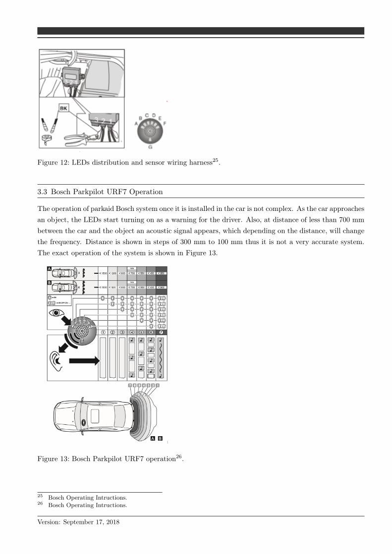
Figure 12: LEDs distribution and sensor wiring harness25.

3.3 Bosch Parkpilot URF7 Operation

The operation of parkaid Bosch system once it is installed in the car is not complex. As the car approachesan object, the LEDs start turning on as a warning for the driver. Also, at distance of less than 700 mmbetween the car and the object an acoustic signal appears, which depending on the distance, will changethe frequency. Distance is shown in steps of 300 mm to 100 mm thus it is not a very accurate system.The exact operation of the system is shown in Figure 13.

Figure 13: Bosch Parkpilot URF7 operation26.

25 Bosch Operating Intructions.26 Bosch Operating Intructions.


4 Bosch Parkpilot URF7 Tests

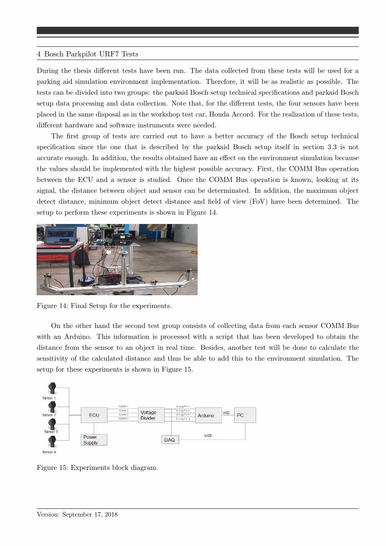
During the thesis different tests have been run. The data collected from these tests will be used for aparking aid simulation environment implementation. Therefore, it will be as realistic as possible. Thetests can be divided into two groups: the parkaid Bosch setup technical specifications and parkaid Boschsetup data processing and data collection. Note that, for the different tests, the four sensors have beenplaced in the same disposal as in the workshop test car, Honda Accord. For the realization of these tests,different hardware and software instruments were needed.

The first group of tests are carried out to have a better accuracy of the Bosch setup technicalspecification since the one that is described by the parkaid Bosch setup itself in section 3.3 is notaccurate enough. In addition, the results obtained have an effect on the environment simulation becausethe values should be implemented with the highest possible accuracy. First, the COMM Bus operationbetween the ECU and a sensor is studied. Once the COMM Bus operation is known, looking at itssignal, the distance between object and sensor can be determinated. In addition, the maximum objectdetect distance, minimum object detect distance and field of view (FoV) have been determined. Thesetup to perform these experiments is shown in Figure 14.

Figure 14: Final Setup for the experiments.

On the other hand the second test group consists of collecting data from each sensor COMM Buswith an Arduino. This information is processed with a script that has been developed to obtain thedistance from the sensor to an object in real time. Besides, another test will be done to calculate thesensitivity of the calculated distance and thus be able to add this to the environment simulation. Thesetup for these experiments is shown in Figure 15.

Figure 15: Experiments block diagram.


4.1 Hardware and Software

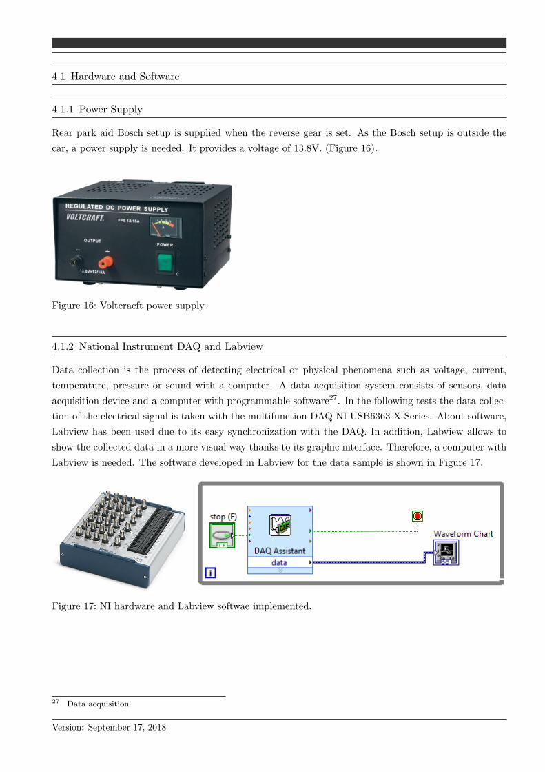
4.1.1 Power Supply

Rear park aid Bosch setup is supplied when the reverse gear is set. As the Bosch setup is outside thecar, a power supply is needed. It provides a voltage of 13.8V. (Figure 16).

Figure 16: Voltcracft power supply.

4.1.2 National Instrument DAQ and Labview

Data collection is the process of detecting electrical or physical phenomena such as voltage, current,temperature, pressure or sound with a computer. A data acquisition system consists of sensors, dataacquisition device and a computer with programmable software27. In the following tests the data collec-tion of the electrical signal is taken with the multifunction DAQ NI USB6363 X-Series. About software,Labview has been used due to its easy synchronization with the DAQ. In addition, Labview allows toshow the collected data in a more visual way thanks to its graphic interface. Therefore, a computer withLabview is needed. The software developed in Labview for the data sample is shown in Figure 17.

Figure 17: NI hardware and Labview softwae implemented.

27 Data acquisition.


4.1.3 Arduino

Arduino is an open source electronic platform based on hardware and software. Arduino will be themicrocontroller chosen for the tests since it has the following advantages in comparison to others:1.) The university owns an Arduino.2.) As an open source platform, there are many resources available on Internet.3.) Compared to other one development boards, Arduino and related products are relatively cheap butalso of excellent quality.4.) Instructions in the Arduino software language are not complex, with basic programming knowledgeone can apply Arduino quickly.5.) The program code is loaded directly on the Arduino board through a USB cable.6.) Its technical specifications are powerful enough for the application to be carried out.7.) Multi platform. The Arduino programming environment is executable in Windows, Macintosh OSXand Linux28.

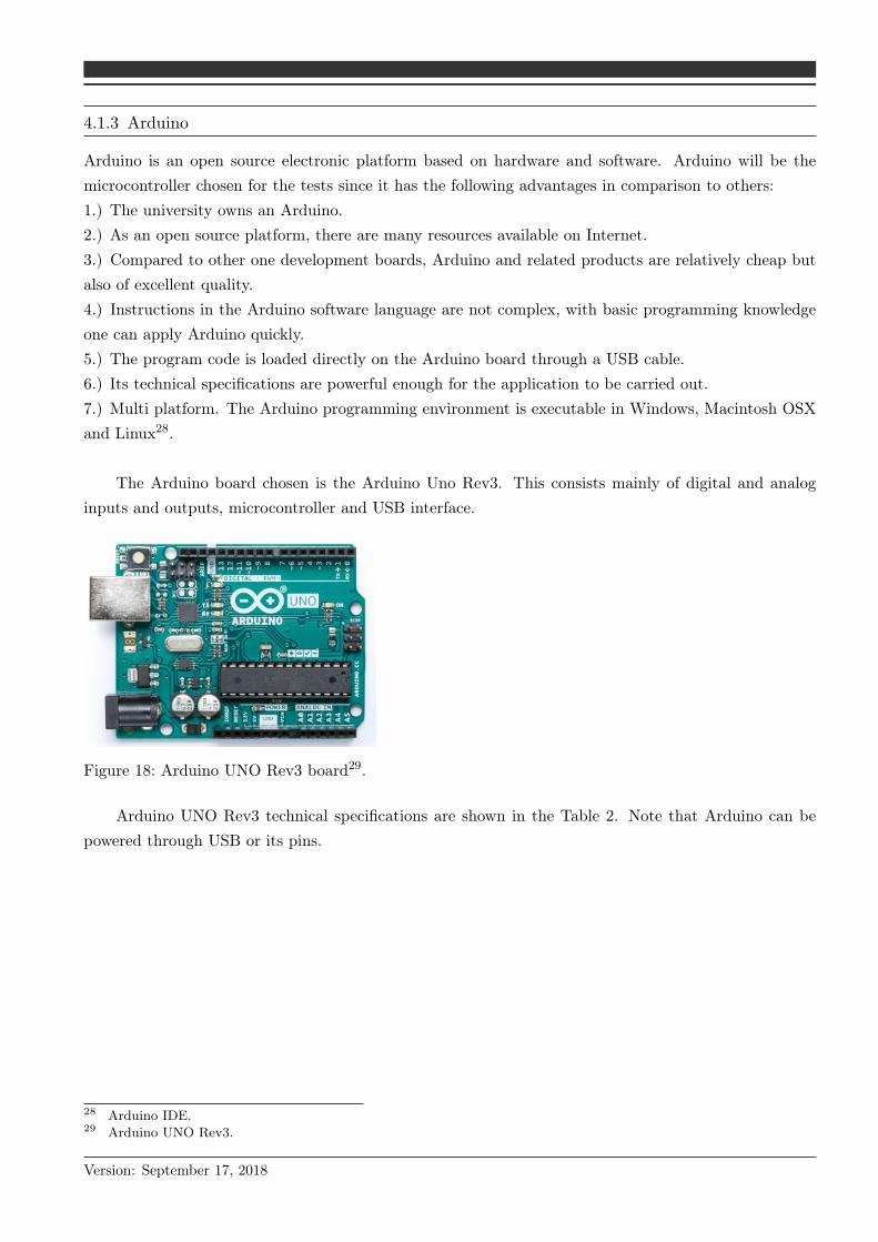
The Arduino board chosen is the Arduino Uno Rev3. This consists mainly of digital and analoginputs and outputs, microcontroller and USB interface.

Figure 18: Arduino UNO Rev3 board29.

Arduino UNO Rev3 technical specifications are shown in the Table 2. Note that Arduino can bepowered through USB or its pins.

28 Arduino IDE.29 Arduino UNO Rev3.


Table 2: Arduino UNO Rev3 technical specifications30.

microcontroller Atmega328P

Operating Voltage 5V

Input Voltage (recommended) 7-12V

Input Voltage (limit) 6-20V

Digital I/O Pins 14

Analog Input Pins 6

DC Current per I/O Pin 20mA

DC Current for 3.3V Pin 50mA

Flash Memory 32 KB

SRAM 2 KB

EEPROM 1 KB

Clock Speed 16 Mhz

Arduino IDE is the software that is used by default for programming with Arduino. This softwareuses a simplified C and C++ language, since it has different libraries included. It is based on theProcessing environment as well as a programming language based on Wiring. The Arduino IDE comeswith a code editor and integrates gcc as a compiler31.

4.1.4 Static Tests Setup

A setup previously assembled by other students is used to fix the sensors position during the experimentsand thus simulate the bumper of a car (Figure 19). The front bar of this setup has been modified in sucha way that the sensors are located in the same position as institute’s Honda Accord test car. Therefore,distances have been taken between the four rear sensors of the car and a new front bar has been designed.Note that the base can be moved small distances and the front bar can take different angles thanks to arotating mechanism.

Figure 19: Previous static tests setup32.

31 Arduino IDE.32 Fu, J. et al.: Setup for ultrasonic models validation (2017)


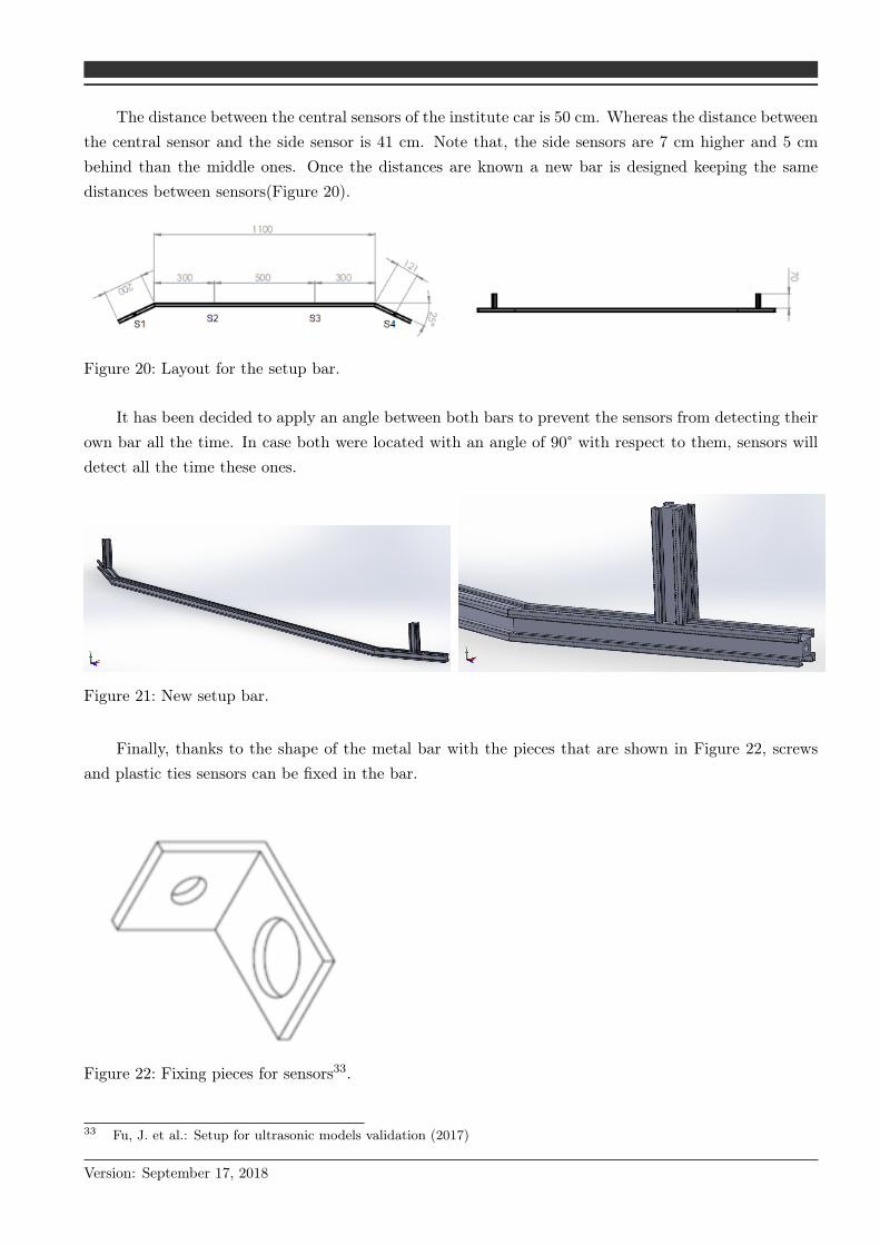
The distance between the central sensors of the institute car is 50 cm. Whereas the distance betweenthe central sensor and the side sensor is 41 cm. Note that, the side sensors are 7 cm higher and 5 cmbehind than the middle ones. Once the distances are known a new bar is designed keeping the samedistances between sensors(Figure 20).

Figure 20: Layout for the setup bar.

It has been decided to apply an angle between both bars to prevent the sensors from detecting theirown bar all the time. In case both were located with an angle of 90° with respect to them, sensors willdetect all the time these ones.

Figure 21: New setup bar.

Finally, thanks to the shape of the metal bar with the pieces that are shown in Figure 22, screwsand plastic ties sensors can be fixed in the bar.

Figure 22: Fixing pieces for sensors33.

33 Fu, J. et al.: Setup for ultrasonic models validation (2017)


4.2 COMM Bus Operation

Once the system is powered, that is, the reverse gear is set, the sensors and ECU module are ready towork. To calculate the distance both ECU and sensors communicate through the COMM Bus. Whenthis is initialized, large amount of data is sent by the ECU to the sensors. During this initialization ECUis responsible for assigning certain level of voltage gain to them. After this, the communication betweenboth ECU and sensors starts. In this communication, two types of pulses can be distinguished accordingto their voltage. Thanks to this, it can be determined which one sensor or ECU is talking in the bus.Then, when the ECU is active on the COMM Bus, it pulls the voltage from the Bus down from 8V to1V . While the sensor, when is active, pulls the voltage down to 1.5V. During this communication, theCOMM Bus signal of one of the sensors is observed with the Labview. The ECU activates each of thesensors with a ping, then the sensor sends the ultrasound signal, which is viewed as a lower voltage pulseon the COMM Bus, to detect if there is any object. In case there is an object the sensor will receive andecho. Otherwise the sensor will wait a specific time, which is called Time of Flight(TOF), and then thesame process will be repeated again.

Figure 23: COMM Bus signal different pulses.

4.3 Distance Measurement Test

The objective of this test is to measure the distance from one of the set up sensors to an object. Therefore,the remaining three sensors are turned away to avoid influencing the signal of the active sensor. For thisexperiment, the COMM Bus data is collected and analyzed. First, the COMM Bus signal is seen whenthe sensor has no object to detect. In this case the signal is shown in Figure 24. The signal is periodic.In each period, four pulses are distinguished. Due to its voltage, three come from the ECU and onefrom the sensor. The sensor pulse is equivalent to the ultrasonic signal sent by itself to detect an object.Since there is no object, the sensor receives nothing. The pulse before the sensor is sent from the ECUto activate the sensor.

Figure 24: COMM Bus signal no object detection.


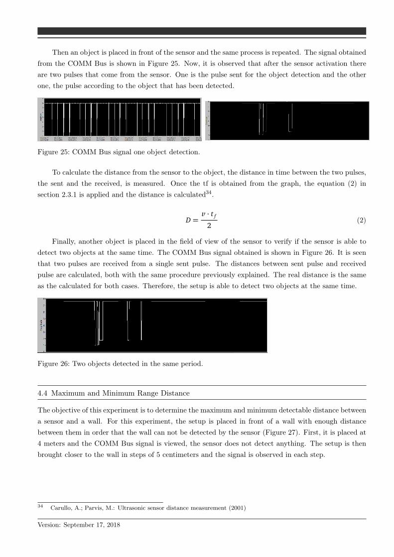
Then an object is placed in front of the sensor and the same process is repeated. The signal obtainedfrom the COMM Bus is shown in Figure 25. Now, it is observed that after the sensor activation thereare two pulses that come from the sensor. One is the pulse sent for the object detection and the otherone, the pulse according to the object that has been detected.

Figure 25: COMM Bus signal one object detection.

To calculate the distance from the sensor to the object, the distance in time between the two pulses,the sent and the received, is measured. Once the tf is obtained from the graph, the equation (2) insection 2.3.1 is applied and the distance is calculated34.

D =v · t f

2(2)

Finally, another object is placed in the field of view of the sensor to verify if the sensor is able todetect two objects at the same time. The COMM Bus signal obtained is shown in Figure 26. It is seenthat two pulses are received from a single sent pulse. The distances between sent pulse and receivedpulse are calculated, both with the same procedure previously explained. The real distance is the sameas the calculated for both cases. Therefore, the setup is able to detect two objects at the same time.

Figure 26: Two objects detected in the same period.

4.4 Maximum and Minimum Range Distance

The objective of this experiment is to determine the maximum and minimum detectable distance betweena sensor and a wall. For this experiment, the setup is placed in front of a wall with enough distancebetween them in order that the wall can not be detected by the sensor (Figure 27). First, it is placed at4 meters and the COMM Bus signal is viewed, the sensor does not detect anything. The setup is thenbrought closer to the wall in steps of 5 centimeters and the signal is observed in each step.

34 Carullo, A.; Parvis, M.: Ultrasonic sensor distance measurement (2001)


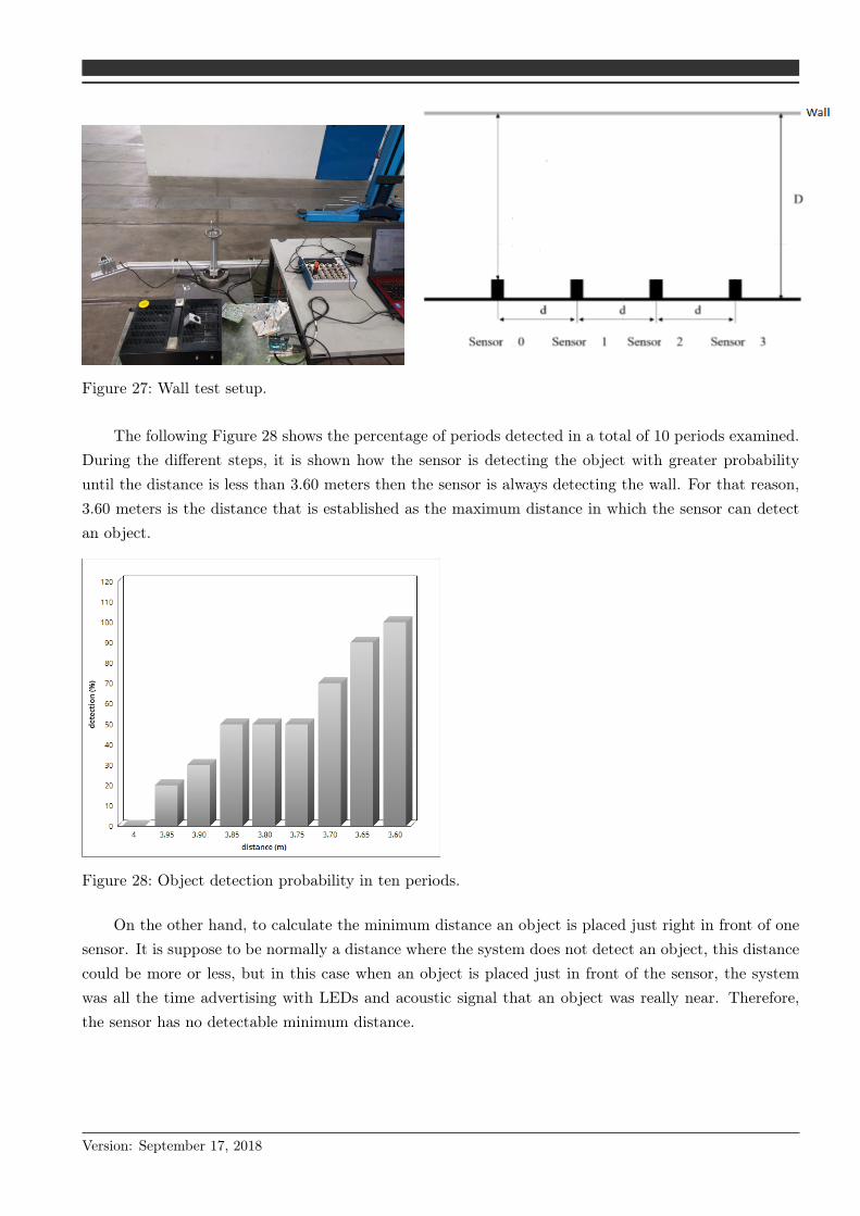
Figure 27: Wall test setup.

The following Figure 28 shows the percentage of periods detected in a total of 10 periods examined.During the different steps, it is shown how the sensor is detecting the object with greater probabilityuntil the distance is less than 3.60 meters then the sensor is always detecting the wall. For that reason,3.60 meters is the distance that is established as the maximum distance in which the sensor can detectan object.

Figure 28: Object detection probability in ten periods.

On the other hand, to calculate the minimum distance an object is placed just right in front of onesensor. It is suppose to be normally a distance where the system does not detect an object, this distancecould be more or less, but in this case when an object is placed just in front of the sensor, the systemwas all the time advertising with LEDs and acoustic signal that an object was really near. Therefore,the sensor has no detectable minimum distance.


4.5 Sensor Field of View Determination

The objective of this experiment is to determine the field of view and the cross echo operation for asensor and for the whole parkaid Bosch setup. In the procedure of this experiment a point object isused to determine both. An object is placed at a distance d and it is moved parallel through the X axis(Figure 29)35. The first point at which the sensor detects the object is fixed as the limit of the sensorfield of view. To fix the other side, the same procedure is repeated. To calculate the angle of this point,a trigonometric relationship is applied that is given by the following equation (3):

β = tan−1 x

d

(3)

Figure 29: Field of View experiment procedure.

To determine the sensor field of view, the experiment explained before has been carried out. In thisexperiment the Figure 14 setup has been used and all the sensors except one have been turned awayto avoid the cross-echo. The experiment has been run for two different positions of the sensor, havinga difference between them of 90° (Figure 30)36. Therefore, both the vertical and the horizontal field ofview have been determined.

Figure 30: Sensor position to determine both FoV.

35 Fu, J. et al.: Setup for ultrasonic models validation (2017)36 Bosch Ultrasonic Sensor.


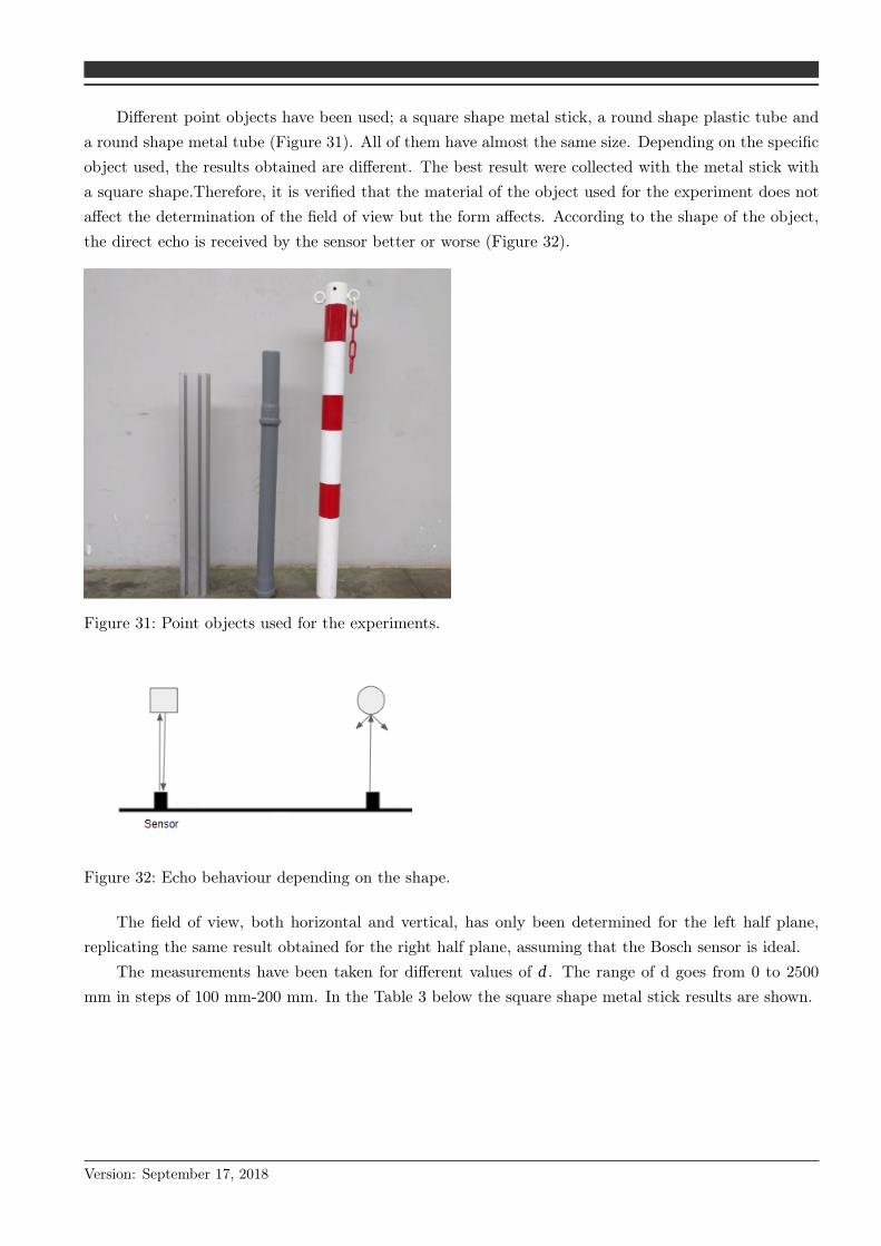
Different point objects have been used; a square shape metal stick, a round shape plastic tube anda round shape metal tube (Figure 31). All of them have almost the same size. Depending on the specificobject used, the results obtained are different. The best result were collected with the metal stick witha square shape.Therefore, it is verified that the material of the object used for the experiment does notaffect the determination of the field of view but the form affects. According to the shape of the object,the direct echo is received by the sensor better or worse (Figure 32).

Figure 31: Point objects used for the experiments.

Figure 32: Echo behaviour depending on the shape.

The field of view, both horizontal and vertical, has only been determined for the left half plane,replicating the same result obtained for the right half plane, assuming that the Bosch sensor is ideal.

The measurements have been taken for different values of d. The range of d goes from 0 to 2500mm in steps of 100 mm-200 mm. In the Table 3 below the square shape metal stick results are shown.


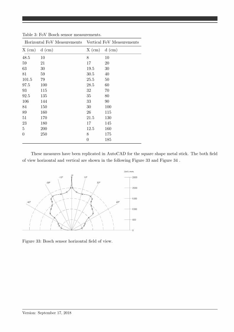
Table 3: FoV Bosch sensor measurements.

Horizontal FoV Measurements Vertical FoV Measurements

X (cm) d (cm) X (cm) d (cm)

48.5 10 8 1059 21 17 2063 30 19.5 3081 59 30.5 40101.5 79 25.5 5097.5 100 28.5 6093 115 32 7092.5 135 35 80106 144 33 9084 150 30 10089 160 26 11551 170 21.5 13023 180 17 1455 200 12.5 1600 250 8 175

0 185

These measures have been replicated in AutoCAD for the square shape metal stick. The both fieldof view horizontal and vertical are shown in the following Figure 33 and Figure 34 .

Figure 33: Bosch sensor horizontal field of view.


Figure 34: Bosch sensor vertical field of view.

4.5.1 Cross Echo Operation

The cross echo occurs when a sensor receives the signal bounced by an object and this signal came fromanother sensor.

To detect the cross echo in the COMM Bus, first an object is placed in front of one of the setupsensors, in such a way that this object is not detected by any of the other sensors in the setup. Thesensor’s 1,3 and 4 signal COMM Bus is watched with Labview Figure 24. Therefore, the sensors are notdetecting any object, while the signal of sensor 2 shows that it detects an object (Figure 25). This firstconfiguration is done just to compare the COMM bus signal when it is detecting a cross-echo.

Figure 35: Cross-Echo Setup.

To facilitate the detection of a cross echo, an object is placed between sensor 1 and sensor 2 (Fig-ure 35). While watching the COMM Bus signal of sensor 2 it can be seen that a period is formed by fivepulses that come from the ECU instead of three.


Figure 36: COMM Bus signal cross echo for different scenarios.

In the left picture of Figure 36, it is presented the COMM Bus signal of a sensor in a cross echoscenario where that sensor is receiving a cross echo from another sensor and also its own echo. It isknown because after the last two large pulses it can be viewed two short pulses, the sent and its ownecho whereas in the two middle large pulses it can be seen just one short pulse which is the cross echo.On the contrary on the right picture, the performing sensor is just receiving the cross echo.

4.5.2 Whole Setup Field Of View Determination

Even though the field of view of a sensor has been determined, replicating this for each of the four sensorcan not be applied for the whole system field of view. Since for intermediate zones between sensors, asensor is able to receive the cross-echo and not its own echo. Which means that for only one sensor thatobject would be outside of its field of view, while for the whole setup that object would be inside thefield of view. Therefore, the same experiment has been repeated as in section 4.5, but with the foursensors in operation. The four communication buses were observed at the same time to know if any ofthe sensors was receiving its own echo or cross-echo and thus determining the limit of the field of view.This experiment has been done with the metal stick with square shape and the plastic stick with roundshape. The results obtained are the following Figure 37 and Figure 38 .

Figure 37: Whole system FoV metal stick.


Figure 38: Whole system FoV plastic stick.

The measurements have been taken for several values of d, in the case of the metal stick, d has arange of 0-2500 mm in steps of 100 mm-200 mm, while for the plastic stick, d has a range from 0-1600mm in steps of 100 mm-200 mm. The plastic stick range is smaller because the setup can not detect it adistance further than 1600 mm. These measurements have been taken for the three different zones thatare pointed out in both Figure 37 and Figure 38. For zone 1, the reference plane for the measurements isthe one of sensor 1, while for zone 2 and 3 the reference plane is the one of sensor 2. All the sensors BusCOMM signal have been watched at the same time since in zones between sensors, it would be possiblethat a sensor can receive a cross echo and not its direct echo. The right half plane has been replicated,assuming the ideality of the sensors.

Table 4: Metal stick whole FoV measurements.

Zone 1 Zone 2 Zone 3

X (cm) d (cm) X (cm) d (cm) X (cm) d (cm)-44 15 -13 262 5 272-60 30 -37 236 25 285-79 47 -46 221 45 270-88 66 -54 200-92 82 -74 175-96 100 -110 163-114 120 -139 145-96 133-82 152-55 170-40 180-21 200-10 215


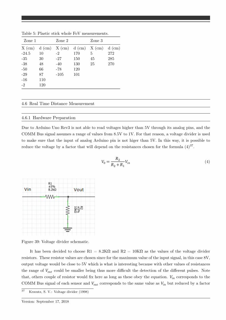
Table 5: Plastic stick whole FoV measurements.

Zone 1 Zone 2 Zone 3

X (cm) d (cm) X (cm) d (cm) X (cm) d (cm)-24.5 10 -2 170 5 272-35 30 -27 150 45 285-38 48 -40 130 25 270-50 66 -78 120-29 87 -105 101-16 110-2 120

4.6 Real Time Distance Measurement

4.6.1 Hardware Preparation

Due to Arduino Uno Rev3 is not able to read voltages higher than 5V through its analog pins, and theCOMM Bus signal assumes a range of values from 8.5V to 1V. For that reason, a voltage divider is usedto make sure that the input of analog Arduino pin is not higer than 5V. In this way, it is possible toreduce the voltage by a factor that will depend on the resistances chosen for the formula (4)37.

V0 =R2

R2 + R1Vin (4)

Figure 39: Voltage divider schematic.

It has been decided to choose R1 = 8.2KΩ and R2 = 10KΩ as the values of the voltage dividerresistors. These resistor values are chosen since for the maximum value of the input signal, in this case 8V,output voltage would be close to 5V which is what is interesting because with other values of resistancesthe range of Vout could be smaller being thus more difficult the detection of the different pulses. Notethat, others couple of resistor would fix here as long as these obey the equation. Vin corresponds to theCOMM Bus signal of each sensor and Vout corresponds to the same value as Vin but reduced by a factor

37 Krzentz, S. V.: Voltage divider (1998)


of 0.55. Therefore, the new range of values is 4.7V-0.55V. Now, Arduino is already able to read the inputsignal of its analog pins. The following figure shows the Arduino schematic (Figure 40).

Figure 40: Arduino connexions.

4.6.2 Software Operation

The software developed calculates the distance between each of the setup sensors to an object in realtime, exactly showing the distance each period T of the COMM signal. Remark that each period T lastsapproximately 250 ms. Arduino reads the COMM Bus signal from each of the sensors and processesit. It means that Arduino detects each of the different pulses, both from the ECU and from the sensorand after a sensor activation by the ECU, if Arduino detects two pulses coming from the sensor, thesent and received, it will calculate the distance in time between them by getting the timestamps of bothpulses with the micros() function. Followed by applying the formula of section 2.3.1, Arduino returnsthe distance value in length units, exactly in centimeters. The micros() function returns the time valuefrom when arduino is turned on until the instant in which the function is called. Besides, the softwaredetects the cross echo but it does not calculate the distance between the sensor that has received thecross echo and the object. Note that the software measurements range goes from 19 cm to 3 m.

Below, there are a tables comparing the actual distance with the measured distance when the objectis placed in a short, medium and long distance from the setup.


Table 6: Measured value for a short actual distance.

Real Distance (cm) Measured Distance (cm)

45 45.3645 45.5045 42.8445 42.7045 45.5045 42.8445 45.5045 45.6445 45.5045 42.84

Table 7: Measured value for a medium actual distance.


125 125.44125 125.58125 125.44125 126125 122.78125 125.58125 125.44125 128.38125 122.78125 125.72


Table 8: Measured value for a large actual distance.


235 235.20235 234.78235 235.62235 232.12235 232.68235 232.12235 232.68235 234.78235 232.68235 234.71

In the tables it is detected that for an actual distance X , the measured distance changes in a rangeof X+-3 cm. Besides, if the actual distance is changed just 1 cm the measured distance still being thesame or jump a 3 cm step. It means that the systems now has a sensibility of 3 cm. With the purposeof fix it a diagnosis has been done and have been concluded that there are three possible cases wherethese errors may come from:

1.) Arduino is not enough fast to detect the change voltage signal, so that Arduino detects the sentpulse with a delay. The equation 1

f = T is used to know how much Arduino needs to take a sample.Arduino works with a f =16Mhz. It means that Arduino takes a sample from the signal each 6,25·10−8s.If the error of the distance measured is 3 cm, maybe Arduino has a delay detecting the received pulse.Applying the equation of section 2.3.1 is known that this 3 cm in time are 0.1765 ms (where v =340 m/s).Therefore, if Arduino takes a sample every 6, 25 ·10−8s, it will take more than one sample in 0.1765 ms.For that reason, Arduino is enough fast and the measurement problem does not come from it38.

2.) The pulse that corresponds to the direct echo hides information in its width. The duration ofthe pulse is measured for different types of objects but the same width result is always obtained, 3.9 ms.Accordingly with the result obtained,the measurement problem does not come from it either.

3.) The direct echo received by the sensor comes from different points where the signal has bounced.Depends on the signal bounced, the distance change its the value. The distance is calculated from morethan one period T without moving the object position and the same distance is obtained always.

With the aim of solving this error in the measurements, it is calculated the arithmetic mean ofthe different values in order to stabilize the final result (5). Consequently, now a final measurement isacquired depending on the selected mean whereas previously a final measurement was obtained for eachperiod T of the COMM signal. The number of period T per final result is equal to N39.

Mean(X ) =−x=

∑Ni=1 X i

N(5)

38 Frequency and Period Time relation.39 Arithmetic Mean Formula.


N has value of 400, 200, 100, 50 and 20 assigned, for long to short distances. In the section 6,results that have been obtained for each N are shown. Note that for each of both N value and kind ofdistance(long, medium or short) has been taken ten samples.

In the results shown, it is observed that the distance from the sensor to the object is not a variableto taken into account. Also, the final measurements are stabilized in all cases, but logically, a greaterstabilization can be seen for the N values of 400 and 200. Finally, the N value chosen for the distancecalculation is N=20. Since for a greater N , too much time is needed by Arduino to show the finalmeasurement and this is not of interest for parking system.

Once the N value is chosen, the software is implemented in order to not calculate the distancebetween an object to a sensor, but the one between object and bumper. For this implementation, theobjects are divided into two groups, large and small. It is assumed that an object is cataloged as largewhen 3 or more sensors are detecting it, whereas when only two sensors detect it, it is classified as small.When a large object is detected, the minimum distance between sensor and object will be shown, since itwill be the same distance between object and bumper Figure 41. While when a small object is detected,the trigonometric relationship of section 2.3.2 will be applied to calculate the distance between the objectand the bumper. In case only one sensor detects an object, the distance shown is the one that goes fromthe sensor to the object.

Figure 41: Example of a large object situation.

4.6.3 Sensitivity Measurement

This experiment consists of determining the sensitivity of the setup. Note that, with setting the sensitivyof the system you also set the accuracy accordingly and it will be implemented in the environment sim-ulation. As software initial condicions for this experiment it does not contain the last part implementedabout the distance from the bumper to an object. Besides, the N value set is 400, since now the delay inobtaining the final measurement does not matter and it is useful to have a result as stable as possible.

The procedure consists of placing an object at a X distance and take the result measured by Arduino.Followed by moving the setup 2 mm away from it, this is possible thanks to the rotating mechanismthat the moveable platform of the setup has. Once the 2 mm are moved, the result are recalculatedby Arduino. The process is repeated in steps of 2 mm until the measurement obtained by Arduino haschanged to the next measurement step. Depends on this step, the sensitivity of the system based on theactual measurement is determinated. Finally it is viewed that when is changed 1 cm from the actualdistance, the next measured step changes 1 cm as well.


This process has been repeated for long, medium and short distances and the results obtained arein the following Table 9, Table 10 and Table 11:

Table 9: Short distance sensitivity experiment results.

Actual Distance (cm) Measured Distance (cm)

44.8 43.6145 43.6345.2 43.9345.4 44.0745.6 44.7345.8 44.8946 45.43

Table 10: Medium distance sensitivity experiment results.


112.8 111.95113 112.17113.2 112.31113.4 112.45113.6 112.72113.8 112.87114 113.11

Table 11: Long distance sensitivity experiment results.


224.8 223.92225 224.36225.2 224.65225.4 224.70225.6 224.96225.8 225.26226 225.28

Due to the volatility for units smaller than the centimeters, it is decided to establish 1 cm as thesensitivity of the system. Note that the results obtained will be always one centimeter less than theactual distance.


5 Conclusions

Once the methodology was followed and the different experiments were elaborated, the results that wereobtained, will be discussed below.

Regarding the field of view (FoV) determination experiment, it should be noted that the experimenthas been carried out with three different objects, in particular: a round shaped metal stick, a roundshaped plastic stick and a square shaped metal stick. In addition, it was experimented with a squareshaped wooden stick, but the experiment could not be validated for the reason that its thickness wasconsiderable and the FoV could not be determined with accuracy. Once obtained the results with thedifferent point objects, it has been concluded that the material does not affect the FoV determination,but the form alters the result seeing that for a square shape better results have been obtained. This isbecause the echo of the signal sent by the sensor is easier to receive when it bounces on a square objectthan a round one. The results achieved are the following: a horizontal FoV of 60 degrees and verticalaround about 30 degrees and a maximum length of 2.6 m as well. About the FoV width , the resultshave been similar to what was expected, while the FoV length has been better than expected in previousstudies.

With respect to the experiment of maximum and minimum length, it has been viewed that the Boschsensor is able to detect objects at a distance of 4 meters, but is not very reliable since at these distancesit is not able to detect the object at 100% of the time. Therefore, to achieve 100% effectiveness, themaximum distance detectable by the sensor is reduced to 3.6m. Note that in this experiment a greatermaximum length has been obtained than in the FoV experiment because in this experiment the setuphas been placed in front of a wall and not a point object, so that the wall is easier to detect due to itssize.

On the other hand it has also been demonstrated if these sensors have implemented the cross echodetection. The cross echo is the signal that comes from another sensor after it has bounced on anobject. During the experiments, its operation has been confirmed, in such a way that with the crossecho functionality implemented, the whole sensor setup FoV improves.

Finally, the calculation of the distance between object and sensor has been tested in such a way thatthe result obtained was as accurate as possible. This has been achieved without any problem readingthe communication signal between sensor and control unit. Later, the script implementation for Arduinowas carried out, which was able to calculate the distance to an object in real time without having toobserve the communication Bus signal. Initially, the results obtained had an measurement failure about3 cm with respect to the actual measurement approximately, even though this failure was not alwaysobtained in the measurement. To solve this error in the measurement, it has been proposed to calculatethe average of N results to get a mean value measured and thus improve the measure accuracy, reachinga maximum error of 1 cm. This mean calculation implementation is used to get a better sensitivity aswell.

To sum up, remark that the Bosch sensors are very powerful which is not reflected in the user-levelfunctionality. It is because a parking assistance system does not require this accuracy and these wideranges of vision. On the other hand, a system for autonomous driving need it, and according to theresults obtained, Bosch sensors are good to do it. Emphasize that all the information or results collected


during the experiments are good enough to create a simulation environment for valet parking use casesthat contribute to autonomous driving.

As aspects to improve, results more reliable could have been obtained if the sensors had beeninstalled in the car. Since in the test setup an attempt has been made to imitate Honda’s bumper interms of distance between sensors, both vertical and horizontal, but the exact sensor orientation couldnot be replicated.

Finally, the work to be carried out in the future could be to develop dynamic tests, possibly withthe sensors in the car, since the experiments have been run in static. The information of which could beimplemented to improve the simulation environment.


6 annexes

Figure 42: Samples medium distance and N=20.

Figure 43: Samples medium distance and N=20.

Figure 44: Samples large distance and N=20.


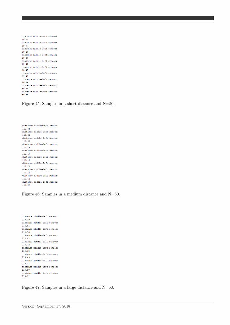
Figure 45: Samples in a short distance and N=50.

Figure 46: Samples in a medium distance and N=50.

Figure 47: Samples in a large distance and N=50.


References

Arduino IDE. Arduino IDE. URL: https://www.arduino.cc/en/Main/Software.Arduino UNO Rev3. Arduino UNO Rev3 Tech Specs. URL: https://store.arduino.cc/arduino-uno-rev3.

Arithmetic Mean Formula. URL: https://en.wikipedia.org/wiki/Arithmetic_mean.Bosch Operating Intructions. Bosch operating intructions. 2009.Bosch Ultrasonic Sensor. URL: https://www.bosch-mobility-solutions.com/en/products-and-services/passenger-cars-and-light-commercial-vehicles/driver-assistance-systems/

construction-zone-assist/ultrasonic-sensor/.Carullo, A. et al.: Ultrasonic sensor distance measurement (2001)

Carullo, Alessio; Parvis, Marco: Ultrasonic sensor for distance measurement in automotive applications,in: IEEE Sensors journal, 1, p. 143, (2001)

Data acquisition. Data acquisition. URL: https://www.ni.com/data-acquisition/d/.Frequency and Period Time relation. URL: https://en.wikipedia.org/wiki/Frequency.Fu, J.: Diss., Ultrasonic sensor model (2018)

Fu, Junfeng: Auswahl und Implementation eines Ultraschall-Sensormodells für die Fahrzeuganwen-dung, (2018)

Fu, J. et al.: Diss., Setup for ultrasonic models validation (2017)Fu, Junfeng; She, Jiahao; Shen, Liwen; Wanf, Qin,; Zuo, Yueyao: Aufbau eines geeigneten Test-Setupszur Validierung von Ultraschallsensor-Modellen, (2017)

Jaffe, B.: Piezoelectric ceramics (2012)Jaffe, Bernard: Piezoelectric ceramics, Elsevier, (2012)

Kishonti, L.: Real and simulated tests (2017)Kishonti, László: In autonomous driving, real-world testing is taking a backseat, (2017)

Krzentz, S. V.: Voltage divider (1998)Krzentz, Steven V: Resistance voltage divider circuit, Google Patents, (1998)

Nakamura, K.: Ultrasonic applications (2012)Nakamura, Kentaro: Ultrasonic Transducers: Materials and Design for Sensors, Actuators and medicalapplications, Elsevier, (2012)

Navarro: Ultrasonic distance measurement (2004)Navarro: Sensores de Ultrasonido usados en Robótica Móvil para la Medición de Distancias, in: Scientiaet Technica, 273, (2004)

Olympus, N.: Ultrasonic Transducers (2006)Olympus, NDT: Ultrasonic transducers technical notes, in: Technical brochure: Olympus NDT,Waltham, MA, pp. 40–50, (2006)

Real and Simulation car tests. URL: https://mashable.com/2017/07/14/autonomous-driving-real-cars-simulations/?europe=true#FSNdrlOXsgqS.

Rubio, C.: Ultrasonic transducer (2010)Rubio, Carlos: Fabricación de Transductores Ultrasónicos para Equipos automatizados de inspecciónde líneas de Tuberías, (2010)

Rubio, C.: Diss., Ultrasonic transducer for automated sytems (2018)Rubio, Carlos: Transductores Ultrasónicos para Equipos automatizados, (2018)

Winner, H.: Handbook of Driver Assistance Systems (2014)Winner, Hermann: Handbook of Driver Assistance Systems, ISBN: 978-3-319-09840-1, (2014)

Yang, C. E.: Piezo electric effect (2016)Yang, Carmen Emily: What is the piezo electric effect?, (2016)


https://www.arduino.cc/en/Main/Software

https://store.arduino.cc/arduino-uno-rev3

https://store.arduino.cc/arduino-uno-rev3

https://en.wikipedia.org/wiki/Arithmetic_mean

https://www.bosch-mobility-solutions.com/en/products-and-services/passenger-cars-and-light-commercial-vehicles/driver-assistance-systems/construction-zone-assist/ultrasonic-sensor/



https://www.ni.com/data-acquisition/d/

https://en.wikipedia.org/wiki/Frequency

https://mashable.com/2017/07/14/autonomous-driving-real-cars-simulations/?europe=true#FSNdrlOXsgqS

https://mashable.com/2017/07/14/autonomous-driving-real-cars-simulations/?europe=true#FSNdrlOXsgqS

implementation and integration of an experimental vehicle

Documents