implementation and validation of the spalart …

ICAS 2002 CONGRESS

IMPLEMENTATION AND VALIDATION OF THESPALART-ALLMARAS TURBULENCE MODEL FOR HIGH

SPEED FLOWS

R. Marsilio, D. GrilloDIASP-Politecnico di Torino, Corso Duca degli Abruzzi 24, 10129 TORINO - ITALY

Keywords: Turbulence Modeling,Air Breathing Propulsion

Abstract

The aim of this paper is to develop an axysim-metric numerical procedure, easily extendible to3-D configurations, based on the Reynolds av-eraged Navier-Stokes equations coupled with aturbulence model to compute the external flowof a plug nozzle. The governing equations arediscretized in the physical domain according afinite-volume technique with second order accu-racy. The turbulence equation written in integralform is solved together with the flow equations.Complex shock-slip surfaces, shock-boundary-layer interactions appear in the flowfield and allthe flow discontinuities will be numerically cap-tured.

1 Introduction

Since the direct numerical simulation of turbu-lence is not possible for practical flow prob-lems due to computer limitations, and as large-eddy simulation has not yet become a practi-cal tool in aerodynamics, the only way to simu-late high speed and high Reynolds-number flowsis to solve the Reynolds-averaged Navier-Stokes(RANS) equations together with a turbulencemodel. Turbulence modeling has become oneof the key problems in CFD. In aerodynamics,simple algebraic turbulence models have beenwidely used with fair success. However, the alge-braic model are not suitable for handling complexflow situations including flow separation, mul-tiple surfaces with turbulent regions near each

other, or wakes etc. Therefore, the developmentof turbulence models has been most intensive inthe area of transport equation models. The modeldevelopment has gone towards physically morerealistic models on the one hand, to increasingcomplexity on the other hand.

In practical aerodynamics, a gap has appearedbetween simple algebraic models with many re-strictions and complex transport equation modelswith difficulty of use and many anomalies. Theidea behind the Spalart-Allmaras model [11] isto fill this gap by creating a ”local” type trans-port equation model, which is more sophisticatedthan algebraic models, but more robust and eas-ier to use than traditional two-equation, or higherdegree model. Here the term ”local” means thatthe equation at one point does not depend on thesolution at the other points. A typical example ofnon locality is found in the algebraic Baldwin-Lomax model, where the maximum value of acertain function is found by traversing throughthe boundary layer and this maximum value isthen used as a model parameter. The searchfor the maximum is typically performed alonggrid lines perpendicular to the boundary layer.Therefore, these kinds of models are only suitedto structured and sufficiently orthogonal grids,and to rather simple boundary-layer-type flows.A local-type model does not suffer from sucha restriction and is thus much better suited tohandling complex flow problems, where multi-ple surfaces, multiple boundary layers, separatedflow regions, free shear layers or wakes occur.

1

R. MARSILIO, D. GRILLO

This paper discusses the implementation ofthe Spalart-Allmaras turbulence model to a nu-merical methodology developed to solve com-plex two-dimensional or axisymmetric flowsconfigurations, [6]. The numerical approach pre-sented is based on a time-dependent integrationof the full Navier-Stokes equations where thephysical domain is discretized according to afinite volume technique. The convective partof the equations (inviscid fluxes) is treated fol-lowing a flux difference splitting method withan approximate solution of a Riemann problemat each cell interface [8], [5]. The diffusiveterms (viscous fluxes) are calculated using a cen-tered scheme. Second order accuracy is achievedfollowing the guidelines of the essentially non-oscillatory schemes (ENO) [2], with linear recon-struction of the solution inside each cell and ateach step of integration. Complex shock-shockand shock-slip surface interactions appear in theflow fields. In our methodology all the shocksand the slip surfaces are numerically captured.

To validate the functionality of the Spalart-Allmaras model the numerical method has beenused to solve the turbulent flat plate boundarylayer and to solve the turbulent flow over abackward-facing step [7].

All the numerical results carried-out havebeen compared with theoretical, experimentaland direct numerical simulations (DNS) data.The performances of the model in complex flowsituations involving shear layer, shock-boundarylayer interactions and recirculating flows will betested by studying the geometry proposed by ON-ERA [10] for turbulent flows validation where theexperimental data are available for comparison.

2 Numerical Method

2.1 Governing Equations

Compressible viscous flows are governed by theNavier-Stokes equations and in particular bythe Reynolds-Averaged Navier-Stokes (RANS)equations coupled with the one-equation turbu-lent equation. All this set of equations may bewritten in a compact integral conservative form

as:

∂∂t

�

v

�Wdv��

s

�FI ��nds��

s

�FV ��nds ��

v

�Hdv

(1)where v represents an arbitrary volume en-

closed in a surface s. System (1) can be re-duced to non-dimensional form with the help ofthe following reference values: L for length, ρ∞for density, T∞ for temperature,

�RT∞ for veloc-

ity, RT∞ for energy per unit mass and µ∞ for vis-cosity. Therefore, from now the flowfield vari-ables should be considered as non-dimensional.In particular, �W is the hyper-vector of conser-vative variables, tensor �FI contains the inviscidfluxes, tensor �FV contains the viscous fluxes andtensor �H contains the non-homogeneous part ofthe equations due to the turbulent model:

�W � �ρ�ρ�q�E� ν̃T�T

�FI ��

ρ�q� p¯̄I�ρ�q��q��E� p��q� ν̃T�q�T

�FV ��

γM∞Re∞

��0�� ¯̄τ��K∇T � ¯̄τ ��q��ν�ν̃T

σ ∇ν̃T

�T

�H �

��0��0��0�cb1S̃ν̃T �

cb2σ �∇ν̃T �

2� cw1 fw�

ν̃Td

�2�T

(2)Quantities ρ, p and �q � �u�v�w�T are the lo-cal density, pressure and velocity, respectively; Erepresents the total energy per unit volume:

E � ρ�

e�q2

2

�(3)

where e is the internal energy per unit mass, M∞and Re∞ are the freestream Mach number and theReynolds number, γ is the ratio of the specificheats, ν̃T is the modified eddy viscosity and fi-nally ¯̄I is the unit matrix. The viscous stresses ¯̄τare contained in tensor , given by:

τi j � µ

�∂q j

∂xi�

∂qi

∂x j� 2

3�∇ ��q�δi j

�ρq��i q��j (4)

The Reynolds-stresses �ρq��i q��j are mod-eled according to the Boussinesq approximation,which allows one to take the Reynolds-stresses

2

Implementation and Validation of the Spalart-Allmaras Turbulence Model for High Speed Flows

into account simply by modifying the viscosity.Thus, the viscous stresses can be written as:

τi j � �µ�µT �

�∂q j

∂xi�

∂qi

∂x j� 2

3�∇ ��q�δi j

(5)

where µT � ρνT is a turbulent viscosity co-efficient obtained from µ̃T � ρν̃T . The thermalconductivity K is calculated in non-dimensionalform as

K �γ

γ�1

�µPr

�µT

PrT

�(6)

where Pr and PrT are the laminar and turbu-lent Prandtl numbers. The laminar viscosity µ iscomputed via Sutherland’s law

µ � T 3�2�

1�Tre f

T �Tre f

�(7)

with

Tre f �110�4

T∞(8)

Finally, the perfect gas relationship p � ρT com-pletes the set of equations.

2.2 Convective and Diffusive Fluxes

The collapse of such a discontinuity generates intime a pattern of waves along which signals prop-agate. The waves split the domain in the vicin-ity of the discontinuity in a set of uniform re-gions where the values of the flowfield variablesare to be computed. Inviscid fluxes �FI are eval-uated defining and solving an appropriate Rie-mann problem across each lateral surface. Thedefinition of the Riemann problem consists, atfirst, in fixing a direction a direction X joiningthe centroids of the two finite volume that areconnected by the considered lateral surface (seeFig.1, left). Then, the variation of the flowfieldvariables along X is to be considered. Due to thediscretization, two piecewise constant (first orderaccuracy Fig.1, right up) or piecewise linear (sec-ond order accuracy, Fig.1, right down) distribu-tions of the flow field variables are present be-tween cells A and B, separated by a discontinuityin correspondence with lateral surface.

I+1/2,J

I+1/2,J

I,J

I+1,J

I+1,J

I,J

I,J

I+1,JA

B

U

U

x

x

y

x

Xηξ

2nd oder

1st order

Fig. 1 Riemann problem

The collapse of such a discontinuity gener-ates in time a pattern of waves along which sig-nals propagate. The waves split the domain inthe vicinity of the discontinuity in a set of uni-form regions where the values of the flowfieldvariables are to be found, generating in this waya Riemann problem. To obtain waves directionsand corresponding signals, the equations govern-ing the inviscid part of the flowfield are writtenin quasi-linear form in a new local frame of ref-erence constituted by direction ξ and η, whichare normal and tangent to the considered lateralsurface, respectively. Here an approximated so-lution of the Riemann problem [8] is sought for,where the shocks which could be generated bythe collapse of the initial discontinuities are ap-proximated by compression waves, but the con-servative form of the equations ensures that thecorrect jump and entropy conditions are satis-fied. Moreover, the Riemann problem is solvedfor simplicity in one spatial dimension rather thantwo, so that only temporal variations of the flow-field variables along the ξ direction are consid-ered. Velocity and temperature gradients neededto evaluate viscous fluxes �FV in correspondencewith lateral surface are computed through a stan-dard technique that uses central differences andapplies the Gauss’s Theorem.

Second order accuracy in space and time isachieved following the guideline of the Essen-tially Non Oscillatory schemes for shock cap-turing technique [2]. No slip and isothermalor adiabatic conditions are applied to the wall.Freestream conditions are enforced at the inlet,while zero-gradient assumed at the exit boundaryfor conservative variables.

3


The eddy viscosity νT is obtained from themodified eddy viscosity ν̃T , which is solved bythe last of the system (1). This equation which ishere called the turbulence equation, is basicallyof similar form to the equations for basic flowvariable: mass, momentum and total energy. Theonly major difference is that the turbulence equa-tion also contains a source term Q inside the vec-tor �H. The basic source term without transitionterms is

Q � cb1S̃ν̃T ��γM∞Re∞

cw1 fw�

ν̃Td

�2�

�γM∞Re∞

cb2σ �∇ν̃T �

2(9)

where the first term represents production andthe second term represents destruction of ν̃T .The third term is called the first-order diffusionterm. The modified magnitude of vorticity is

S̃ � S��γM∞

Re∞

ν̃T

κ2d2 fv2 (10)

where S is the magnitude of vorticity

S �

∂v∂x� ∂u

∂y

(11)

and d is the distance to the nearest wall. Thefunction:

fv1 �χ3

χ3� c3v1

fv2 � 1� χ1�cv1 fv1

(12)

where χ � ν̃T�ν. In the distruction term, fw isdefined as:

fw � g

�1� c6

w3

g6� c6w3

�1/6(13)

where

g � r� cw2�r6� r�� (14)

with

r ��γM∞

Re∞

ν̃T

S̃κ2d2(15)

The model coefficients are:

cb1 � 0�1355� cb2 � 0�6222�

σ � 2�3� κ � 0�41�

cw1 � cb1�κ2��1� cb2��σ� cv1 � 7�1� (16)

cw2 � 0�3� cw3 � 2�0

The eddy viscosity, or turbulent viscosity, neededin the viscous stress tensor (5) is obtained from

µT � ρ fv1ν̃T (17)

As boundary conditions free-stream eddy viscos-ity is specified by setting a value for χ at the free-stream boundaries. Usually it can be set to zero.The eddy viscosity is equal to zero on the sur-faces, so its inviscid flux is also zero on the walls.

3 Model validation

3.1 Boundary layer flow

The first test case, used for validation, corre-sponds to a M∞ � 0�3 flow over an insulated flateplate. In table 1 the freestream conditions for theflow parameters for this case are reported.

M∞ 0.3T∞ 300 KRe�m 106 1/mR 287 J/(Kg K)γ 1.4Pr 0.72PrT 0.90

The viscosity is assumed constant in the flowfield and its value has been computed with theSutherland’s law at 300K. In these conditions theunit Reynolds number is about 106/m. The com-putational domain is a rectangular area wherethe length is 5m whereas the width is 0�2m (seeFig.2)

The dimension of the computational domainis such as to assure a negligible influence on theboundary layer computation. The numerical so-lution has been computed on a 100�50 grid. Themesh is characterized by a wall stretching definedby

y j � h

1�β

ea�1� j∆hh ��1

ea�1� j∆hh ��1

�(18)

4


0 5

0.5

x

y

Fig. 2 Flat plate computational grid

where

∆h �hny

� a ��log

�β�1β�1

�(19)

j being the node index, h the domain width,ny the total number of cells in y-direction, βa stretching parameter whose value has to begreather than 1. In the present test case thestretching parameter value is set at 1.0001. Thisvalue assures that the y� value at the first gridpoint near the wall is approximately 1. Sincefor this test case the freestream Mach numberis very low, the compressibility effects are neg-ligible. For this reason it is possible to comparethe numerical results with incompressible bound-ary layer data. In Fig. 3 the c f distribution isshown as a function of the Reynolds number Rex

based on the properties at the edge of the bound-ary layer and the distance from the leading ledge.

Spalart−Allmaras

Re x

1e + 078e + 066e + 064e + 062e + 060

0:008

0:007

0:006

0:005

0:004

0:003

0:002

0:001

0

Theoretical lawExp. data

Cf

Fig. 3 Turbulent susbsonic boundary layer

The results computed by the code are com-pared with the analytical skin friction coefficient

law for the incompressible turbulent boundarylayer flow:

c f �0�0592�Rx�0�2 (20)

and the experimental c f distribution measured byWieghardt and Tilmann [12]. It is clear that theresults are in good agreement with the referencedata. In Figs. 4 and 5 the u�U∞ and u� profilescorresponding to the test section at x � 0�4m areshown. As reference data have been considered

Spalart−Allmaras

y

0 : 140:120:10:080:060:040:020

1:2

1

0:8

0:6

0:4

0:2

0

Exp. data

u/U θ

Fig. 4 Velocity profile at x � 0�4m

the analytical sublayer law

u� � y� (21)

and the log layer law:

u� �1k

log�y��5 (22)

and the u� profile computed by Wieghardt andTielmann’s experimental data [1]. The dataagreement is excellent.

3.2 Turbulent flow over a backward-facingstep

Separation and reattachment of turbulent flowsoccur in many practical engineering application,both in internal flow systems such as diffusers,combustors and channels with sudden expansionsand external flows like those around airfoils andbuildings. In these situations, the flow experi-ences an adverse pressure gradient, the pressure

5


Spalart−Allmaras

y +

u +

1000010001001010:1

30

25

20

15

10

5

0

Log lawsublam. layer law

Exp. data

Fig. 5 u� profile at x � 0�4m

increase in the direction of the flow, which causesthe boundary layer to separate from solid sur-face. The flow subsequently reattaches down-stream forming a recirculation bubble. Amongthe flow geometries used for the studies of sep-arated flows, the most frequently selected is thebackward/facing step. Considerable work hasbeen carried out on this flow due to its geomet-rical simplicity. For such a reason we used thisgeometry to validate our numerical methodology.Figure 6 shows a schematic view of the flow do-main used in this computation.

y

U

x/h0

h Xr

Fig. 6 Backward-facing step configuration

For semplicity, we used a rectangular compu-tational domain starting at the edge of the step(x � 0). The coordinate system is placed at thelower step corner as shown in Fig. 6. Themean inflow velocity profile u�y�, imposed at theleft boundary (x � 0) is a computed flat-plateboundary layer profile. To validate the computa-tional results the numerical simulations were car-ried out for Reynolds number (Reh � 5100) and

compared with the experimental and DNS results[9], [7], [4]. A stretched computational grid inboth x and y directions was used. The computedmean reattachment length is Xr � 6�0h compa-rable with the experimental Xr � 5�39h, and theDNS, Xr � 6�28h, Xr � 6�0h. The reattachmentlength was demonstrated by Kuen [3] to increaseas the expansion ratio increases.

In Fig. 7, the average Cf is compared withDNS and experimental data. Good agreement is

Spazzini et allJovic−Driver

Le−Moin−KimSpalart−Allmaras

2520151050

0:004

0:003

0:002

0:001

0

0:001

0:002

0:003

0:004

0:005

0:006

0:007

y/h

Cf

Fig. 7 Comparison between computation DNSand experimental

obtained between computational and experimen-tal data. A striking from previous measurementsand the DNS is the large peak of negative skinfriction in the recirculation region see in both inour computation and DNS experiment. The Peaknegative Cf obtained with our method is about2 times larger than other results. The secondaryvortex in the recirculation bubble is smallest. Infact the Spalart-Allmaras model tends to over es-timate the skin friction coefficient when there is alack of points close to the walls. Figure 8 presentsthe comparison between computational results,experimental and DNS data. The comparison ismade st four representative locations in the re-circulation (a), reattachment (b) and recovery re-gions (c) and (d). Figure 9 compares the com-putational results with the DNS measurements atx�h � 19�0. All profiles are below the universallog-law even at 20h downstream of the step. Pre-

6


10 : 80:60:40:200:2

3

2:5

2

1:5

1

0:5

0

(a) = 4 : 0

10:80:60:40:20

3

2:5

2

1:5

1

0:5

0

(b) = 6:0

10:80:60:40:20

3

2:5

2

1:5

1

0:5

0

(c) = 10:0

10:80:60:40:20

3

2:5

2

1:5

1

0:5

0

(d) = 19:0

Jovic−DriverLe−Moin−Kim

Spalart−Allmaras

y/h

u/uo

y/h

y/h y/h

u/uo

u/uo u/uo

x/h x/h

x/h x/h

Fig. 8 Mean streamwise velocity profile

vious experimental studies reported a recovery ofthe log-law profile as early as 6 step heights afterthe reattachment. The good agreement betweenthe computation and DNS profile at x�h � 19�0confirms that the deviation from the univeral log-law is a real effect in this flow. The apparent dis-crepancy between the present near wall profilesand the experiments is attributed to the methodof obtaining the wall-shear velocity uτ.

4 Plug nozzle results

The numerical simulations of plug nozzle con-cern a reference plug geometries based on dif-ferent characteristics of the flow exhausting onthe plug wall. The FLOWNET Test-Case P02,proposed by ONERA for CFD validation [10](P02) has been used. The P02 geometry shownin Fig.10 has been computed with the following

Jovic−DriverLe−Moin−Kim

Spalart−Allmaras

u+

y +

1000010001001010:1

25

20

15

10

5

0

Subvisc. layerLog−law

Fig. 9 Mean streamwise velocity profiles in wallcoordinates at x�h � 19�0

flow conditions, which correspond to the experi-mental ones: for the external flow we have M∞ �

Fig. 10 Flownet Test-Case P02

1�95, stagnation pressure Po � 1� 105 Pa andstagnation temperature of 295K; in the jet flowthe total pressure is 5� 105 Pa and the stagna-tion temperature is 297 K. The Reynolds numberis 12�27� 106, referenced to the external plug-diameter (40mm). All the computations havebeen carried out working with cold air (γ � 1�4).Laminar and turbulent Prandtl number are 0.72and 0.9 respectively. Adiabatic wall boundarycondition has been assumed for the temperature.In Fig.11 the computed Mach number contour-lines are shown. The visualization shows a shockinteracting with the external boundary-layer de-

7


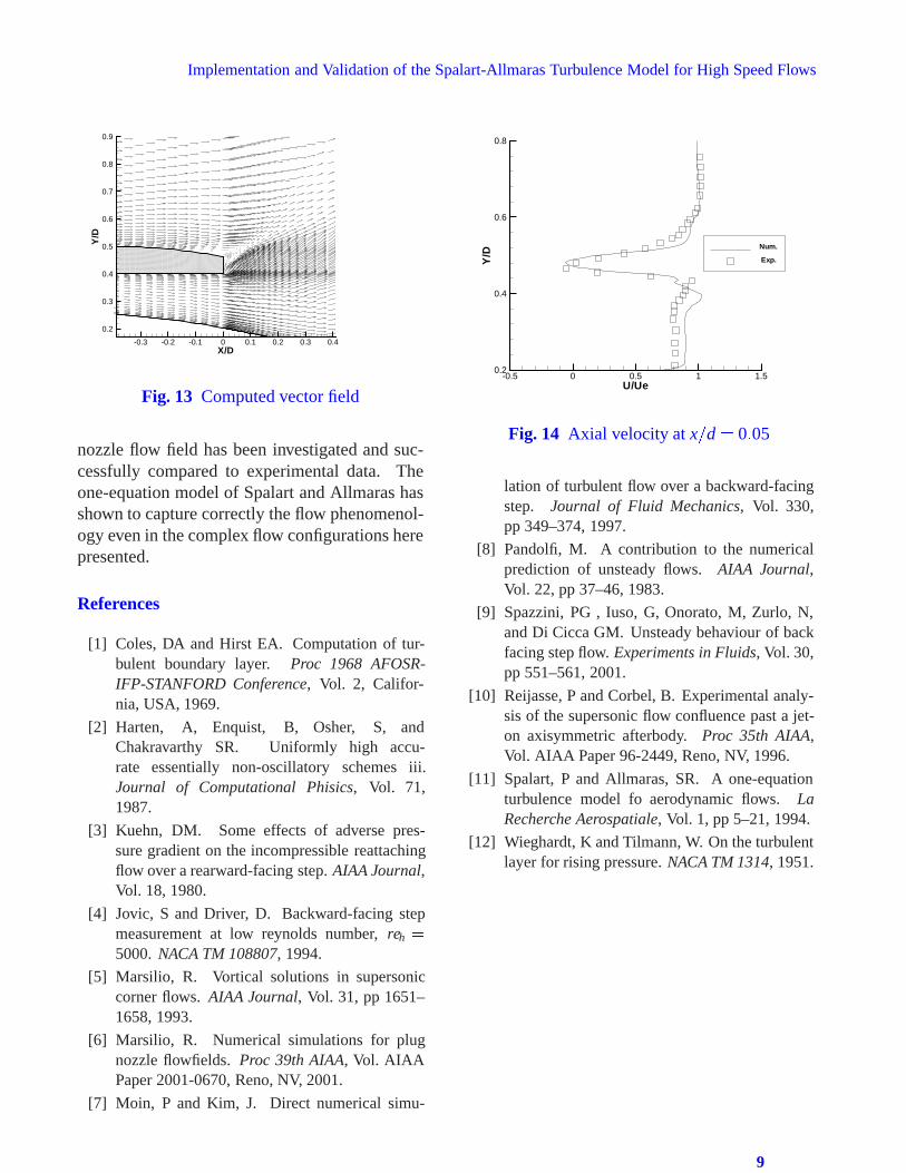
veloping on the boattail. Figure 12 shows thestreamlines patterns. After flow separations, oc-curring near the end of the boattail for the ex-ternal stream and the nozzle lip for the jet, theflow frontiers envelop a dead water region be-fore co-flowing. The confluence process startsthe development of a wake that ensures the mu-tual adaptation of the flow. In the nozzle exit re-gion, we distinguish the expansion fan centerednear the nozzle lip. It is followed by a wave fo-calization process that creates the classical bar-rel shock structure of an underexpanded jet. Aqualitative analysis with the schlieren photographtaken from Ref.[10] shows a good agreement onthe wave behavior. Figure 13 shows a generalview of the coumputed velocity vector field closeto the boat-tail region. It is possible to observethe main flow deviation induced by the crossingof either the outer confluence shock or the barrelshock and the progressive mutual adaption of theco-flowing streams along a wake region and thedevelopment of the mixing layer.

1.98

1.98

1.981.42

2.831.13

3.40

4.25

1.42

X/D

Y/D

-0.5 0 0.5 1

0.5

1

1.5

2

Fig. 11 Mach Number

The comparisons between experimental andnumerical data are shown in Figs. 14, 15, 16and 17. Figures 14 and 15 refer to the compar-ison of the computed turbulent streamwise veloc-ity (straight lines) and the experimental mean ve-locity (squares) [10] at stations x�d � 0�05 andx�d � 0�1. The numerical data for the turbulent

X/D

Y/D

-0.5 0 0.5 1

0.5

1

1.5

2

Fig. 12 Streamlines

case agrees very well with the experimental onesand the recirculating bubble close to the boattailis captured correctly. Figure 16 shows also thecomparisons in terms of the radial velocity com-ponent at the station x�d � 0�05 .

Figure 17 presents a comparison between thewall computed and the experimental pressure onthe boattail, and normalized by the upstreamstatic pressure p∞ The aspect of the pressure dis-tribution on the same generating line is typicalof an interaction between the external boundarylayer and a shock. At first, the approach staticpressure is nearly constant and close to 1. Theflow expansion induced by the boattail makes thestatic pressure decrease. Then, at certain locationX0 between �6 and �10mm, the pressure goesup rapidly when the boundary layer crosses a nar-row compression wave system located at the footof the shock. Figure 18 shows a 3-D sketch ofthe flow pattern. system located at the foot of theshock.

5 Conclusion

A numerical method based on the integration ofthe unsteady Reynolds Averaged Navier-StokesEquation has shown to be a suitable tool for plugnozzle analysis and for investigation of the super-sonic flow past an axisymmetric afterbody.

The numerical solution of a full length plug

8


X/D

Y/D

-0.3 -0.2 -0.1 0 0.1 0.2 0.3 0.4

0.2

0.3

0.4

0.5

0.6

0.7

0.8

0.9

Fig. 13 Computed vector field

nozzle flow field has been investigated and suc-cessfully compared to experimental data. Theone-equation model of Spalart and Allmaras hasshown to capture correctly the flow phenomenol-ogy even in the complex flow configurations herepresented.

References

[1] Coles, DA and Hirst EA. Computation of tur-bulent boundary layer. Proc 1968 AFOSR-IFP-STANFORD Conference, Vol. 2, Califor-nia, USA, 1969.

[2] Harten, A, Enquist, B, Osher, S, andChakravarthy SR. Uniformly high accu-rate essentially non-oscillatory schemes iii.Journal of Computational Phisics, Vol. 71,1987.

[3] Kuehn, DM. Some effects of adverse pres-sure gradient on the incompressible reattachingflow over a rearward-facing step. AIAA Journal,Vol. 18, 1980.

[4] Jovic, S and Driver, D. Backward-facing stepmeasurement at low reynolds number, reh �

5000. NACA TM 108807, 1994.

[5] Marsilio, R. Vortical solutions in supersoniccorner flows. AIAA Journal, Vol. 31, pp 1651–1658, 1993.

[6] Marsilio, R. Numerical simulations for plugnozzle flowfields. Proc 39th AIAA, Vol. AIAAPaper 2001-0670, Reno, NV, 2001.

[7] Moin, P and Kim, J. Direct numerical simu-

U/Ue

Y/D

-0.5 0 0.5 1 1.50.2

0.4

0.6

0.8

Num.

Exp.

Fig. 14 Axial velocity at x�d � 0�05

lation of turbulent flow over a backward-facingstep. Journal of Fluid Mechanics, Vol. 330,pp 349–374, 1997.

[8] Pandolfi, M. A contribution to the numericalprediction of unsteady flows. AIAA Journal,Vol. 22, pp 37–46, 1983.

[9] Spazzini, PG , Iuso, G, Onorato, M, Zurlo, N,and Di Cicca GM. Unsteady behaviour of backfacing step flow. Experiments in Fluids, Vol. 30,pp 551–561, 2001.

[10] Reijasse, P and Corbel, B. Experimental analy-sis of the supersonic flow confluence past a jet-on axisymmetric afterbody. Proc 35th AIAA,Vol. AIAA Paper 96-2449, Reno, NV, 1996.

[11] Spalart, P and Allmaras, SR. A one-equationturbulence model fo aerodynamic flows. LaRecherche Aerospatiale, Vol. 1, pp 5–21, 1994.

[12] Wieghardt, K and Tilmann, W. On the turbulentlayer for rising pressure. NACA TM 1314, 1951.

9


U/Ue

Y/D

-0.5 0 0.5 1 1.50.2

0.4

0.6

0.8

Num.

Exp.

Fig. 15 Axial velocity at x�d � 0�1

V/Ue

Y/D

-0.5 0 0.5 1 1.50.2

0.4

0.6

0.8

Num.

Exp.

Fig. 16 Radial velocity at x�d � 0�05

X (mm)

P/P

e

-40 -35 -30 -25 -20 -15 -10 -5 00.4

0.6

0.8

1

1.2

1.4

Num.

Exp.

Fig. 17 Wall pressure distribution

Y

X

Z

Fig. 18 3-D flow configuration

10

implementation and validation of the spalart …

Documents