Implementation of a Stationary Navier StokesEquation Solver

Florian Reichl, Oliver Meister

September 21, 2007

i

Contents1 Introduction 2

2 Preparation 32.1 Installation . . . . . . . . . . . . . . . . . . . . . . . . . . . . . . . . . 32.2 Using PETSc . . . . . . . . . . . . . . . . . . . . . . . . . . . . . . . . 32.3 Testing . . . . . . . . . . . . . . . . . . . . . . . . . . . . . . . . . . . . 3

3 Wrapping the PETSc Methods 53.1 The Navier-Stokes Equations . . . . . . . . . . . . . . . . . . . . . . . . 53.2 Peano . . . . . . . . . . . . . . . . . . . . . . . . . . . . . . . . . . . . 53.3 The PETSc Nonlinear Solver . . . . . . . . . . . . . . . . . . . . . . . . 63.4 Data Transfer . . . . . . . . . . . . . . . . . . . . . . . . . . . . . . . . 73.5 Peano Adapters . . . . . . . . . . . . . . . . . . . . . . . . . . . . . . . 7

4 Optimization 94.1 Adding Time Steps . . . . . . . . . . . . . . . . . . . . . . . . . . . . . 94.2 Tuning the Jacobian Matrix Calculation . . . . . . . . . . . . . . . . . . 94.3 Configuring the Linear Solver . . . . . . . . . . . . . . . . . . . . . . . 10

5 Conclusion And Prospects 12

A Test Cases 13A.1 Free Channel . . . . . . . . . . . . . . . . . . . . . . . . . . . . . . . . 13A.2 Cylinder Obstacle . . . . . . . . . . . . . . . . . . . . . . . . . . . . . . 14A.3 Driven Cavity . . . . . . . . . . . . . . . . . . . . . . . . . . . . . . . . 15

Bibliography16

1

1 IntroductionAt the ”Lehrstuhl Informatik 5” at the TU Munchen, a research project in the field ofefficient fluid simulation called ”Peano” is being developed. Peano concentrates on in-compressible flows in two and three dimensions and uses a finite element method for theapproximation of the solution to a problem. The API PETSc (Portable Extensible Toolkitfor Scientific Computation) is used for that purpose.

Subject of this project is the implementation of a solver which has the special task offinding those steady state solutions by solving the (discrete) Navier-Stokes Equation im-plicitly. Therefore a wrapper is needed to link the non-linear functionality of PETSc toPeano.

The project itself was divided into seven steps:

1. Familiarization with the problem:The first step was getting familiar with solving non-linear equation systems. Thisincludes collecting several equations which can be used to test a solver’s behaviorin some selected cases.

2. Testing PETSc:The test equations collected in step one should be implemented using PETSc. Sev-eral solution methods are to be tested and compared to each other.

3. Wrapping all necessary PETSc methods:The necessary PETSc methods are wrapped into classes and integrated into thePeano project. These classes have to be consistent with the Peano coding standards.

4. Setting up the Navier-Stokes equations:The continuous stationary Navier-Stokes equations are to be implemented in a dis-cretized form on a regular grid in 2D.

5. Solving several test scenarios:Several test scenarios should be implemented, documented and compared to eachother.

6. Alternative calculation of the Jacobian matrix:If necessary, the calculation of the Jacobian matrix should be optimized.

7. Linking the calculation to the time step based solver:The new solver is linked to the existing one to improve the initial value for betterperformance.

2 Preparation

2.1 InstallationThe first step of the project was getting a windows computer ready to compile Peano. Weused Cygwin 1.5.24-2 on Windows XP SP2 with the gcc 3.4.4 compiler. Make, Pythonand gcc containing g++ and g77 have to be installed.After that, we created two different PETSc builds for debug and release purposes usingthe following commands:

./config/configure.py --with-cc=gcc --with-fc=g77 --download-f-blas-lapack=1--with-mpi=0

./config/configure.py --with-cc=gcc --with-fc=g77 --download-f-blas-lapack=1--with-mpi=0 --with-debugging=0 COPTFLAGS="-O3"

For Peano we had to write our own makefile based on a sample makefile for PETSc sincesome libraries differed from those used under native linux. We included our makefile onthe enclosed CD, so we will abstain from a library listing at this point.

2.2 Using PETScPETSc itself is fairly easy to handle: Basically, all it needs is a pointer to a method thatevaluates a mathematical function f : Rn→ Rn at a point z ∈ Rn. Additionally, one maypass a pointer to another method evaluating the Jacobian function J : Rn→ Rn×n of f inz ∈ Rn - if no such function is given, PETSc offers a set of methods for calculating theJacobian using finite differences.Given these informations and provided an initial value x0 ∈Rn, PETSc tries to find a rootx ∈ Rn of the function f using a Newton technique. Therefore, in the n-th iteration apoint xn ∈ Rn is determined, which should be a closer approximation to x than xn−1. Forthat purpose, J(xn) must be calculated and f - possibly multiple times - evaluated in eachiteration.

2.3 TestingAmongst others we tested the PETSc functionality with the following 2-dimensional func-tion:

f :

R2 → R2

(xy

)7→

(x2−4y+7

3x2 + log(x)−2

) (1)

PETSc offers two different non-linear solvers: the trust region and the line search tech-nique, although the implementation of trust regions is still in an ”experimental” state.

3

Additionally, it turned out to be much slower than line search and was therefore ignoredby us for the rest of the project.Line search is provided with four different variants: ”cubic”, ”quadratic”, ”basic” and”basic with no norms”. As shown in table 1, all line search techniques converge in ap-proximately the same time, though the ”basic with no norms” variant did not deliver anyviable results in any of our tests. Thus we chose to use the cubic variant which is thedefault PETSc method as it is considered the most stable one.

trust region line search - cubic line search - quadratic line search - basictime[s] 0.32363 0.0069520 0.0091453 0.0062743

Table 1: Convergence times

The non-linear solver of PETSc uses an internal linear solver which can also be config-ured, but as stability and performance cannot be judged appropriately for low dimensionalequations like our test equation, we will postpone this topic to section 4.3 and appendixA.1, where the test results of the Navier-Stokes equation are discussed.

4

3 Wrapping the PETSc MethodsAs mentioned in the introduction, Peano uses a finite element method to approximate thesolution of the Navier Stokes equations. Therefore, a discrete grid is needed, which canbe either adaptive or regular.By now only regular grids are supported by the components of this project, so the adap-tive components are ignored in the following explanations though Peano offers supportfor both grid types.

3.1 The Navier-Stokes EquationsThe continuous, incompressible Navier-Stokes equations are defined by

∇ ·u = 0 (2)

(u ·∇) ·u− 1Re·∆u+∇p = 0 (3)

Those equations are discretized, resulting in the following equation:

B(u,p) :=(

M ·uC(u) ·u+D ·u−MT ·p

)= 0 (4)

where

• B : Rm×Rn → R is the discrete Navier-Stokes function, with m being the griddimension times the number of vertices and n the number of cells in the grid

• u is a vector containing the x and y components of the fluid velocity in every gridvertex

• p is a vector containing the pressure value in every cell

• M is an n×m matrix

• D is an n×n matrix

• C is a linear function from Rn to Rn×n

Additionally, we define J : Rm×Rn→ R(m+n)×(m+n) as the Jacobian of B.

3.2 PeanoThe whole Peano implementation is object oriented, therefore all necessary methods haveto be wrapped in classes. Figure 1 shows a simplified layout of the fluid component andthe nonlinear solver component.

5

Figure 1: Simplified Peano class diagram

PETScNonLinearEquations essentially contains the methods evaluating B and J, func-tion() and jacobianGrid(), which are used by the PETScNonLinearSolver class. ThePETScNonLinearSolver class itself is independent of the fluid component - merely apointer to the FluidSimulation class is passed through to function() and jacobianGrid().FluidSimulation contains wrapping methods for access to the grid, whereas their func-tionality is provided by TrivialgridFluidSimulation for regular grids.TrivialgridFluidRunner triggers the calculation in FluidSimulation, deciding whether atime step based or a steady state simulation will be executed.

3.3 The PETSc Nonlinear SolverThe PETScNonLinearSolver class provides wrapper methods for PETSc that can be usedto solve equation systems without detailed knowledge about the PETSc API. The Usageof this class is explained in the doxyS documentation, so we’ll focus on the mathematicaldetails at this point.

When the solver is started, it performs the following actions, described in pseudocode:

Listing 1: PETScNonLinearSolver functionality1 x := i n i t i a l v a l u e

l i n e a r s o l v e r := ”GMRES” or ”LSQR” or ”GMRES wi th SPAI”FOR i = 1 TO maximum number o f n o n l i n e a r i t e r a t i o n s DO

4 Se tup a LSE J ( x ) ∗ d = b ( x ) u s i n g l i n e s e a r c hSo lve LSE u s i n g l i n e a r s o l v e rC a l c u l a t e s t e p wid th lambda

7 x := x + lambda ∗ d

IF t o l e r a n c e c o n d i t i o n s a r e met THEN EXIT FOR

6

10 END FOR

where b(x) is a vector determined by line search.

Note: GMRES with SPAI is not yet supported.

3.4 Data TransferAs PETSc stores its information in vectors, these data have to be passed back and forthfrom and to the Peano grid. In every iteration, the current values for u and p are stored intoan array and uploaded to the grid, where B and J are computed using the existing peanogrid functionality. Once the calculation is complete, B is read from the grid, stored intoan array and handed back to PETSc as a result of the Navier Stokes equations, whereas Jis stored into a matrix and made available to PETSc.

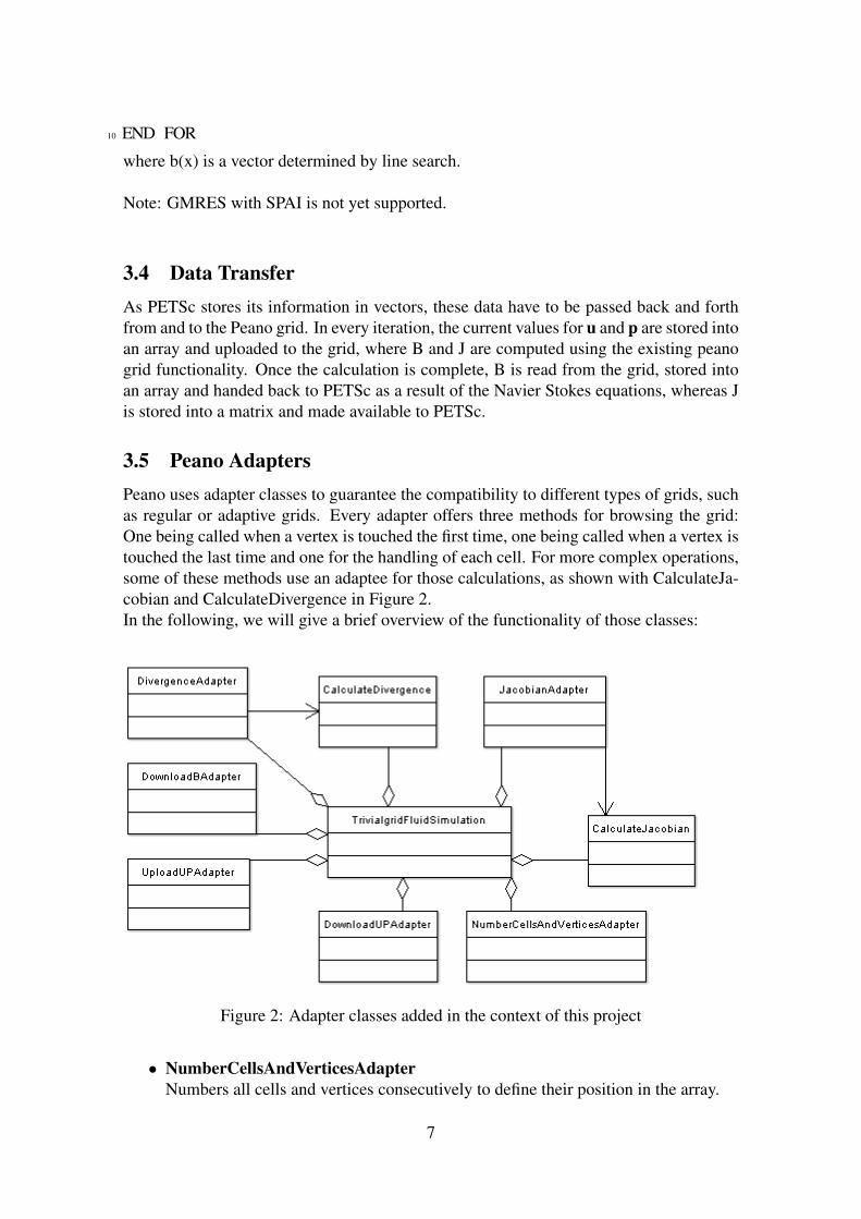
3.5 Peano AdaptersPeano uses adapter classes to guarantee the compatibility to different types of grids, suchas regular or adaptive grids. Every adapter offers three methods for browsing the grid:One being called when a vertex is touched the first time, one being called when a vertex istouched the last time and one for the handling of each cell. For more complex operations,some of these methods use an adaptee for those calculations, as shown with CalculateJa-cobian and CalculateDivergence in Figure 2.In the following, we will give a brief overview of the functionality of those classes:

Figure 2: Adapter classes added in the context of this project

• NumberCellsAndVerticesAdapterNumbers all cells and vertices consecutively to define their position in the array.

7

• DownloadUPAdapterReads current u and p from the grid to create an initial value for PETSc.

• UploadUPAdapterCopies the values of u and p from an array into the grid. This Adapter is calledbefore the calculation begins.

• DivergenceAdapterUses the CalculateDivergence class to calculate the divergence of every cell. Thedivergence in a point is defined by ∇ ·u. In discretized form, this means it’s calcu-lated for a cell by multiplying an element matrix with the velocities of the verticessurrounding the cell and adding up the results.

• DownloadBAdapterDownloads the value of B from the grid into an array. This Adapter is called afterthe calculation of B has finished.

• JacobianAdapterCalculates the Jacobian matrix. This is described in detail in section 4.2.

Note: For the trivial grid, all adapters have the prefix ”TrivialgridEventHandle2” attachedto their names. As adaptive grids are not supported by now, only the trivial grid eventhandle adapters exist.

8

4 OptimizationAs our tests have shown at this point, the implementation was much too slow and partiallyunstable by now, so several optimizations to improve performance and stability were nec-essary.

4.1 Adding Time StepsThe first step to improve the stability was tuning the initial value. In spite of generallyusing 0, Peano performs a number of time steps given by the configuration. The resultingvalues for u and p are used as an initial value for the calculation of the steady state after-wards.After this change the solver worked more stable, as intended, however we could not ob-serve any speed improvements.

4.2 Tuning the Jacobian Matrix CalculationPETSc’s built-in finite differences calculation turned out to be slow as it does not have anyknowledge about the underlying grid of the scenario. Therefore it does not know whichcomponents in the array (u,p) contribute to one component of B(u,p) and assumes thatall entries do when in fact only a small number does, which is independent of the grid size(≤ 22 values per component for 2D).

It is possible in PETSc to color the matrix columns for a more efficient calculation, butthis optimization works only to a certain degree. There is still a lot of obsolete calculationwhich can be avoided.

The final matrix has the following layout:

J =

∂imp1

∂u1

∂imp1∂u2

∂imp1∂p

∂imp2∂u1

∂imp2∂u2

∂imp2∂p

∂div∂u1

∂div∂u2

∂div∂p

where:

• u1, u2 are x, y components of u

• p = pressure values

• imp1, imp2 are x, y components of the discrete impulse equation left hand side (seechapter 3.1, second component of B(u,p) in equation (4))

• div = divergence values

9

Note that ∂div∂p = 0 for the whole block, as the divergence is independent of the pressure.

We considered two simple options how to arrange u and p in the input array: either as(u,p) (variant A) or (p,u) (variant B), of which variant A proved to be more stable thanB. Though it might seem odd that we deliberately chose to set a large number of diagonalentries to 0, the advantage of variant A lies in all other diagonal entries being guaranteednon-zeros. Variant B has neither the advantage nor the disadvantage of variant A, but ithas a higher probability of zero diagonal entries.

As mentioned before, it is only necessary to compute the influence on each component ofB(u,p) for a limited number of components of (u,p). For div in a cell these are u1 and u2of the vertices adjacent to the cell (≤ 8 for 2D). For imp1 and imp2 in a vertex v these areall velocities of the vertices that share a cell with v (≤ 9 ·2 = 18 for 2D) and the pressurevalues of the surrounding cells (≤ 4 for 2D).

We use finite differences for the computation, so for a function f and scalar x, ∂ f∂x would

be calculated as f (x+h)− f (x)h . The default value for h is 10−7 if ||x||< 1, else ||x|| ·10−7.

So at first, we calculate ∂div∂u1

and ∂div∂u2

where div is calculated on a cell c and u1 and u2 arechanged on all the vertices surrounding the cell c.

Next, we calculate ∂imp1∂p and ∂imp2

∂p where p is changed on the cell c and imp1 and imp2are calculated on all the vertices surrounding the cell c.

Finally, for every pair of vertices (v, w) that share the cell c, we calculate ∂imp1∂u1

, ∂imp1∂u2

,∂imp2

∂u1and ∂imp2

∂u2where u1 and u2 are changed on v and imp1 and imp2 are calculated on

w. The resulting values are added to the Jacobian entries.’Added’, because all vertices surrounding all cells adjacent to a vertex w contribute to thederivation in w, not just those of one cell. So the added contributions of each cell result inthe derivation.

The result was a speed increase of the Jacobian calculation of up to factor 5 in comparisonto the standard method, which confirmed our assumptions.

4.3 Configuring the Linear SolverAs mentioned in section 2.3, the PETSc non linear solver uses an internal linear solverwhich can be extracted and configured. Initially a least squares linear solver was used- this method solves the system AT ·A · x = AT · b. Its advantage lies in its stability, asAT ·A is guaranteed not to have zeros in the diagonal if the rank of A is full. However thismethod usually converges slowly, as κ(AT ·A) = κ(A)2.We added the possibility to use GMRES as a linear solver instead. This method solvesthe system A ·P−1 ·P ·x = b using right side ILU(dt) preconditioning. ILU(dt) is a variantof the ILU preconditioning method which drops values beneath a certain tolerance forimproved performance and less memory requirement. As demonstrated in appendix A.1,this solver offers a better performance than LSQR for most problems and should therefore

10

be used if possible.

Here, we were able to increase the overall computation speed up to a factor of 4.

11

5 Conclusion And ProspectsIn conclusion, one can say that all set goals have been achieved satisfactorily. Most testcases were solved with adequate stability, precision and speed, although there are still afew stability issues that could be addressed.By now, the calculation of the steady state is limited to 2D regular grids, the solver isalready prepared to handle adaptive and / or higher dimensional grids. The CalculateJa-cobian adapter would have to be extended to support higher dimensions, whereas it shouldrequire no changes for the adaptive grid. CalulateDivergence, PETScNonLinearEquationsand the trivialgrid adapters would also need to be extended, but this should be a minoreffort.Parts of the functionality provided by TrivialgridFluidSimulation could also be moved toits super class FluidSimulation to support both grid types.

12

A Test CasesAll test cases were run on a AMD Athlon 64 3500+ (2,20 GHz) with 2 GB RAM un-der Windows XP SP2, using a release build of both Peano and PETSc. We chose threedifferent scenarios to present: The free channel, a channel containing a cylinder-shapedobstacle and the driven cavity scenario.

A.1 Free ChannelThis scenario was chosen mostly to show the difference between the GMRES and LSQRlinear solver. As you can see, using GMRES results in a much faster calculation for thisexample. Also an analytical solution exists for this scenario, so we had the possibility ofvalidating the correctness of our computation.

Configuration: resolution 220 x 41, Re = 20, relative tolerance = 10−7

Figure 3: Free channel steady state

linear solver runtime number of iterationsGMRES 61 s 3

LSQR 283 s 19

Table 2: Test results free channel

13

A.2 Cylinder ObstacleFor this scenario, a reference value for the forces that affect the cylinder obstacle exists(see [2]). Thus it offers an excellent opportunity to check the precision of the computedsolution, as also small differences which do not show up in other tests are noticeable.

Configuration: resolution 440 x 82 and 220 x 41, Re = 20, relative tolerance = 10−7

Figure 4: Cylinder obstacle, resolution 220 x 41

resolution runtime number of iterations force vector x force vector y220 x 41 73 s 4 0.00991225 4.21583 ·10−05

440 x 82 760 s 4 0.00941885 2.21526 ·10−05

Force reference 0.01116 2.14 ·10−05

Table 3: Test results cylinder obstacle

14

A.3 Driven CavityAlthough this scenario does not provide any further information, we included it just toverify the functionality of our solver through an additional test.

Configuration: resolution 81 x 81, Re = 1, relative tolerance = 10−7

Figure 5: Driven cavity steady state

test case runtime number of iterationsDriven cavity 39 s 2

Table 4: Test results driven cavity

15

References[1] http://www-unix.mcs.anl.gov/petsc/petsc-as/.

[2] M. Schafer and S. Turek. Flow Simulation with High-Performance Computers II, vol-ume 52 of Notes on Numerical Fluid Mechanics, chapter Benchmark Computationsof Laminar Flow Around a Cylinder, pages 547–566. Vieweg, 1996.