implementation of continuum-based plasticity …gvsets.ndia-mich.org/documents/mstv/2014...such a...

UNCLASSIFIED: Distribution Statement A. Approved for public release

UNCLASSIFIED: Distribution Statement A. Approved for public release

2014 NDIA GROUND VEHICLE SYSTEMS ENGINEERING AND TECHNOLOGY

SYMPOSIUM MODELING & SIMULATION, TESTING AND VALIDATION (MSTV) TECHNICAL SESSION

AUGUST 12-14, 2014 - NOVI, MICHIGAN

IMPLEMENTATION OF CONTINUUM-BASED PLASTICITY FORMULATION FOR VEHICLE/SOIL INTERACTION IN MULTIBODY

SYSTEM ALGORITHMS

Ulysses Contreras Computational Dynamics Inc

Berwyn, IL

Antonio M. Recuero Department of Mechanical and

Industrial Engineering University of Illinois at Chicago

Chicago, IL

Ashraf M. HamedDepartment of Mechanical and


Chicago, IL

Cheng Wei

Department of Aerospace Engineering, Harbin Institute of

Technology Harbin, China

Craig FosterDepartment of Civil and Materials

Engineering University of Illinois at Chicago

Chicago, IL

Paramsothy Jayakumar U.S. Army RDECOM-TARDEC

Warren, MI

Michael D. Letherwood U.S. Army RDECOM-TARDEC

Warren, MI

David J. Gorsich U.S. Army RDECOM-TARDEC

Warren, MI

Ahmed A. ShabanaDepartment of Mechanical and


Chicago, IL

ABSTRACT

Recent advances in the capabilities of personal, workstation, and cloud computing platforms have spurred developments in many computational fields. Terramechanics, involving the study of the dynamic interactions between vehicle and terrain, could, to great benefit, leverage existing compute power towards the use of higher fidelity models. In this paper, we outline the formulation and implementation of an inelastic continuum based soil model in a multibody system (MBS) simulation environment. Such a new computational environment will allow for the simulation of the complex and dynamic interactions occurring at the interface between tracks and wheels, and the ground. The soil model is developed using the absolute nodal coordinate formulation (ANCF) finite elements. In deformable terrain, soil is modeled as a set of 8-node brick ANCF elements whose mechanical behavior may be defined by a suitable constitutive model. A Drucker-Prager plasticity material, which is used to model the behavior of the soil, is proper for the simulation of a number of types of soils and offers a good starting point for computational plasticity in terramechanics applications. Such higher fidelity terramechanics simulations can be fruitfully applied towards the investigation of complex dynamic phenomena in terramechanics. The proposed ANCF/Drucker-Prager soil model is implemented in a MBS computer code. This implementation is demonstrated using an Armored Personnel Carrier (APC) model.

1. INTRODUCTION

The mechanical behavior of soils depends on many factors including the loading and soil conditions. The accuracy of the solution of the vehicle/soil interaction problems for given loading conditions depends on the assumptions used in and the details captured by the specific model. As reported by [1], some approximations are based on simple discrete elastic models that do not capture the distributed elasticity and inertia of soil. On the other hand, more detailed soil models employ a continuum mechanics approach that

captures the soil elastic and plastic behaviors. The successful implementation of continuum mechanics-based soil models requires the use of finite element (FE) algorithms. Nonetheless, existing MBS commercial computer programs cannot be used to study vehicle/soil interaction using continuum based soil models. This is mainly due to the challenging problems encountered in the implementation of continuum-based soil models in computational MBS algorithms. The successful integration of continuum-based soil models with MBS algorithms is necessary in order to be

Proceedings of the 2014 Ground Vehicle Systems Engineering and Technology Symposium (GVSETS) UNCLASSIFIED: Distribution Statement A. Approved for public release

Implementation of Continuum-Based Plasticity Formulation for Vehicle/Soil Interaction in Multibody…, Contreras, et al. UNCLASSIFIED: Distribution Statement A. Approved for public release

of 19

able to develop more detailed and more accurate vehicle/terrain dynamic interaction models. This work aims at integrating a variety of physics-based phenomena making use of an MBS framework. Using this approach, complex multibody systems which may comprise mechanical components modeled as flexible bodies, such as a tracked vehicle, can interact with flexible ground. The deformation of the soil may be described using any of the available soil formulations, whose equations are solved within the same framework as the MBS vehicle model. This approach avoids the use of co-simulation techniques and simplifies significantly the building of the vehicle/soil models.

In this paper, a continuum-based Drucker-Prager soil model that can be integrated with computational MBS algorithms is developed. In the procedure described in this paper, the elastic/plastic soil forces are determined using numerical integration. ANCF finite elements will be used to model the soil deformation. ANCF Cholesky coordinates are employed leading to an identity inertia matrix associated with the Cholesky generalized coordinates [2]. The MBS system algorithm for solving the resulting tracked vehicle/soil dynamic equations is also described.

This paper is organized as follows. Section 2 highlights the state of the art of soil modeling from a vehicle/soil interaction viewpoint and discusses its main challenges. The Drucker-Prager yield function and its associative flow rule are detailed in Section 3. Section 4 describes some necessary modifications to the expressions shown in Section 3 aiming to include linear hardening of the plastic material; this section also provides some basic expressions for non-associative plastic flow. Section 5 gives an overview on the absolute nodal coordinate formulation (ANCF) and summarizes the definition of elastic-plastic material forces that will be used in the section of numerical results. Section 6 is devoted to analyzing the form and terms of the equations of motion, which include a MBS model of the tracked vehicle and its interaction with the elastic-plastic soil. The algorithms used for solving perfect and linear hardening plasticity are discussed in Section 7. The numerical results, contained in Section 8, analyze the motion of the vehicle and elastic-plastic deformation of the soil under the passage of a tracked vehicle. Several soil parameters are considered to determine their influence on the final deformation. Finally, conclusions and future work are summarized in Section 9.

2. SOIL MODELING CHALLENGES AND

STATE OF THE ART Developing a high fidelity vehicle/soil model is necessary

in order to capture important details of the interaction between tires or tracks and soil. This can be a very challenging task, particularly if continuum-based soil models are used. When dealing with continuum-based soil models, the following issues must be addressed [1]:

Strength and deformation characteristics: Shearing of soil materials can have a significant impact on its deformation characteristics and shear strength. Due to interlocking effects, some soils demonstrate an increase in shear strength directly proportional to an increase in mean stress (or applied pressure). In contrast, sands often exhibit an increase in density as the interlocking behavior increases. Other phenomena, such as grain crushing or pore collapse, contribute to soil failure or yielding at very high mean stresses. Plasticity behavior: Soils often exhibit a very small elastic region. Beyond or near the elastic limit the soil undergoes irrecoverable deformation. The inelastic behavior of soils differs between soil types and compositions of each type (amount of gasses and liquids present in the soil). Strain-hardening/softening: A change in the size, shape, and location of the yield surface of the soil can indicate strain-hardening or strain softening behavior. Dense granular materials and over-consolidated clays exhibit strain-softening during dilation, while loose granular materials and normally consolidated clays exhibit strain-hardening during compaction.

Other issues of soil modeling, such as tensile strength, temperature dependency, and drainage effects, etc., can be important in particular simulation scenarios. Moreover, the particularities of the kinematics of plastic deformation require special attention to finite elements technology [3].

The simulation of the interaction between soft soil and vehicle (or vehicle components) has been studied by a number of researchers. For a summary of simulations composed of rigid and deformable tires on soft terrain, see [4] or [5]. Examples of finite element based simulation of terramechanics applications can be found in [6-12]. For an example of a full vehicle on soft soil refer to [13].

The main goal of this paper is to develop continuum mechanics-based soil models and discuss its integration with FE/MBS simulation algorithms. The paper also explains how this FE soil/MBS vehicle integration can be achieved. The literature is weak in this area because there are few investigations that are focused on the use of continuum-based soil mechanics in the study of the vehicle/terrain interaction. This weakness of the literature was supported by many facts as discussed by [1].

3. DRUCKER-PRAGER MODEL

In this section, the Drucker-Prager plasticity model used in this investigation is described. The Drucker-Prager model is based on the strain additive decomposition, and therefore, can be used in the case of small soil deformations [14].

Basic Plasticity Equations

The elastic constitutive equations used in this small deformation model are



of 19

: eσ = E ε (1) where σ is the second-order stress tensor, E is the fourth

order tensor of elastic coefficients, and eε is the second order elastic Green-Lagrange strain tensor. Using the assumptions of the additive strain decomposition, one can write the total strain tensor ε as e p ε ε ε , where pε is the second-order plastic strain tensor. The yield function for the Drucker-Prager model can be written as [15]

1

3tf Q P P (2)

In this yield function,

6e ev sP K , Q G (3)

where K is bulk modulus, G is the elastic shear modulus,

tP is a constant of isotropic hardening parameter, is a

constant, P is the hydrostatic pressure, Q is a deviatoric

stress invariant, ev is the volumetric elastic strain, and

e es s ε is the deviatoric elastic strain norm. Equation (2)

defines a smooth surface in the principal state space as displayed in Figure 1. The following equation shows some basic relations necessary to compute algorithmically Eqs. (2) and (3):

1 3 3tr

3 2 21

tr3

e e e e ev s v

P ( ), Q P ,

P ,

σ σ I S

S σ I ε ε ε I (4)

where S is the deviatoric stress tensor. The flow rule based on associative plasticity may

be defined by the following relationship:

p f

εσ

(5)

in which is the consistency parameter or plastic

multiplier rate.

Solution Algorithm It is assumed that the total strain ε is known from the

solution of the system equations of motion. Therefore, the system of plasticity equations that consist of the constitutive equations, the flow rule, and the yield function has the following unknowns: σ , pε and . If the consistency

parameter can be determined, the plastic strains pε can be

determined using the flow rule. Knowing the plastic strains and the total strains, the elastic strains eε can be determined and used to evaluate the stress tensor σ .

The efficient solution of the plasticity equations presented in this section can be accomplished by reducing these equations to one linear equation which can be solved for the consistency parameter. Note that

tre e e pv : : ε I ε I ε ε , and consequently

pP K : I ε ε . It follows that

pP K : K : f σI ε ε I ε (6)

One can also write

e e e e p ps s s s s s s s: : ε ε ε ε ε ε ε , which upon

differentiation with respect to time leads to

1

1 1

3

e e es s se

s

p p ps s se

s

:

: :

ε εε

ε ε ε ε I ε Iε

(7)

Using the flow rule, one has

1 1

3e ps s s se

s

: f : f

σ σε ε ε I Iε

(8)

Using the yield function and the fact that in the plastic

region 0f , one has the following equation:

1

2 03

e es vf Q P G K (9)

The preceding two equations and the flow rule lead to

2 1

3

0

ps s sp

s s

GF f : f : f

K : f

σ σ

σ

ε ε ε I Iε ε

I ε

(10)

This equation can also be written as

1

3

0

ps s s

ps s

F : f : f

: f

σ σ

σ

ε ε ε I I

ε ε I ε

(11)

Dividing by ps sε ε , one has

Figure 1: Drucker-Prager yield surface in principal stress space and P-Q space.



of 19

1

3

0

sˆF : f : f

: f

σ σ

σ

n ε I I

I ε

(12)

where 2K G , and e e p ps s s s s s

ˆ n ε ε ε ε ε ε .

It is shown in Appendix A (Equation (A.10)) that

2

2

2

1

3 22

e trtrs

sne trs

trtr tr tr

tr

ˆ , G ,

f , J :J

σ

εS Sn S S ε

S ε S

SI S S

(13)

Therefore, the equation for F is a linear algebraic equation in which can be solved in a straight forward

manner to determine the consistency parameter as

1

3

sˆ : :

ˆ ˆ: f : f : : f

σ σ σ

n ε I ε

n I n I I

(14)

Knowing the value of and recognizing that n̂ and fσ

can be expressed in terms of the trial state which is based on information from the previous step, one can make the assumption that the plastic strain rate p f ε σ

remains constant over a given time increment. For most loading scenarios, this assumption is an approximation, and

f σ must be chosen at a given point in the time interval

to create an approximate solution. This allows for having closed form integration for the flow rate equation

p f ε σ as

p p

n

ft

ε εσ

(15)

Knowing the plastic strain pε and the total strain ε , the

elastic strain e p ε ε ε can be determined and used in the calculation of the stress tensor σ . The stress tensor σ can be used in the formulation of the elastic forces. The plastic

state is determined using 2tr tr tr

tf J P P , where

2 2tr tr trJ : S S as defined in Appendix A, and

3trvn

P P KI I ε= + .

An Alternate Approach

As another alternative to the procedure proposed in the preceding section for the solution of the Drucker-Prager plasticity equations is described in this section. Nonetheless, similar results to Eq. (15) can be obtained.

By letting , one has the following three rate

equations:

1

3

e p

s

f,

ˆ : :

ˆ ˆ: f : f : : f

σ σ σ

σ = E : ε εσ

n ε I ε

n I n I I

(16)

These equations can be solved for the unknowns ,σ ε , and . Note that the preceding equations lead to

1 1

3

e p p p

n n n

sn n

f: : : ,

ˆ : :

ˆ ˆ: f : f : : f

σ σ σ

σ = σ E ε E ε E ε ε εσ

n ε I ε

n I n I I

(17)

Again, the approximation that f σ is constant is used

here, and some approximation must be employed. Using the third expression in Eq. (17), one can determine which

can be substituted in the second equation to determine pε

from which p p p

n ε ε ε can be determined. Using this

result, the current stress state can be determined as

e

n n

f: : :

σ = σ E ε E ε Eσ

. Note that the

second equation p p

nf ε ε σ in the preceding

equation when substituting t implies linear

variation of the plastic strain, which is the same result previously given by Eq. (15).

The above algorithms, based on 0f are currently not

favored in plasticity modeling. The primary reason for this is that the approximation in f σ results in the stress state

drifting from the yield surface during plastic flow. This drift can result in spurious non-smooth stress evolution in the numerical results.

4. ISOTROPIC LINEAR HARDENING AND NON-ASSOCIATIVE PLASTICITY

The perfect plasticity model previously presented can be modified to capture linear or nonlinear hardening. In this section, we present the modifications necessary for linear isotropic hardening. The majority of what follows is based on the mathematical theory of plasticity. Interested readers can consult, for example, [14, 16, 17]. Moreover, a non-associative plastic flow rule is described at the end of this section.

Non-Linear Hardening

Strain hardening and work hardening are two approaches that are often used to describe isotropic hardening. The most frequently used choice of strain hardening is considered [17]. In this case, a scalar hardening internal variable is



of 19

selected as an appropriate measure of the strain. A typical selection for this hardening internal variable is the accumulated plastic strain defined as [14]

0 0

2 2

3 3

t tp p p p: dt dt ε ε ε (18)

At the smooth portion of the cone, the evolution of the accumulated plastic strain is given by [14]

p (19)

where is a material constant. Similarly, at the apex, the

evolution of the accumulated plastic strain is governed by volumetric strain changes

p pv

(20)

The above equations are taken as the definitions of the evolution of the hardening internal variable, the accumulated plastic strain, of associative hardening Drucker-Prager model. It is convenient for Drucker-Prager plasticity with hardening to formulate the yield function as an explicit function of the cohesion of the material. It is assumed that

tP c , where c is the cohesion defined as the intercept

of the Mohr-Coulomb failure envelope of the material with the shear axis (shown in Figure 1 for a Drucker-Prager yield surface). The dependence of the cohesion with accumulated plastic strain can be defined using the linear equation

0p pc c H , where 0c and H are constants chosen

to approximate experimentally obtained material hardening response. The modified yield function is then given by

1

3

pcf Q P

(21)

This function can be written at the current time step as

1

1 1 1

1

3

p

n

n n n

cf Q P

(22)

The substitution of the return mapping update equations into the above equation results in

1

1

13

3

0

tr

n

p

ntr

f Q G

cP K

(23)

Substitution of the discretized flow rule, for the smooth portion of the cone, gives us a scalar equation in one unknown. The solution for is

2 2

trf

G K H

(24)

Similarly for the apex of the Drucker-Prager cone, one has

1

1 1 1

10

3

p

n

n n n

cf Q P

(25)

Since at the apex 10

nQ

, the above equation reduces

to

1

10

p

n

n

cP

(26)

Upon substitution of the return mapping update equations, it follows that

0 0tr p p pv vn

P K c H

(27)

Substitution of the discretized flow rule, for the apex of the cone, leads to a scalar equation in one unknown. The solution for p

v is

0

2

tr p

np

v

P c H

H K

(28)

More details on the case of linear hardening are presented in Appendix B of this paper.

Non-Associative Flow rule

The over-prediction of dilation in soil materials can be mitigated by the consideration of a non-associative flow rule. Non-associative flow rules, in contrast to associative flow rules, do not require normal (perpendicular) return mapping to the yield surface. This non-normality violates the principle of maximum plastic dissipation, but is necessary to accurately predict dilation in soils. Replacing the flow rule with

p g

εσ

(29)

where g is normally taken to be a function analogous to the yield surface, and all other variables are as previously defined. In this instance, g is taken as

1

3g Q P b (30)

where and b are constants. For non-associative linear

hardening flow, the increment of the plastic volumetric strain can be shown to be

0

2

tr p

np

v

P c H

H K

(31)



of 19

The plasticity algorithms presented below can be modified with the above considerations to account for non-associative material response.

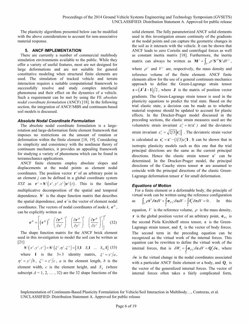
5. ANCF IMPLEMENTATION

There are currently a number of commercial multibody simulation environments available to the public. While they offer a variety of useful features, most are not designed for large deformations and are not suitable for general constitutive modeling when structural finite elements are used. The simulation of tracked vehicle and terrain interaction requires a suitable computational framework to successfully resolve and study complex interfacial phenomena and their effect on the dynamics of a vehicle. Such a requirement can be met by using the FE absolute nodal coordinate formulation (ANCF) [18]. In the following section, the integration of ANCF/MBS and continuum-based soil models is discussed.

Absolute Nodal Coordinate Formulation

The absolute nodal coordinate formulation is a large-rotation and large-deformation finite element framework that imposes no restrictions on the amount of rotation or deformation within the finite element [18, 19]. Considering its simplicity and consistency with the nonlinear theory of continuum mechanics, it provides an appealing framework for studying a variety of phenomena which can be found in terramechanics applications.

ANCF finite elements employ absolute slopes and displacements at the nodal points as element nodal coordinates. The position vector jr of an arbitrary point in an element j can be defined in a global coordinate system

XYZ as j j j j j jx , y ,z tr S e . This is the familiar

multiplicative decomposition of the spatial and temporal dependence. jS is the shape function matrix that describes

the spatial dependence, and je is the vector of element nodal

coordinates. The vectors of nodal coordinates of node k, jke , can be explicitly written as

TT T Tjk jk jk

Tjk jkj j jx y z

r r re r (32)

The shape function matrix for the ANCF brick element used in this investigation to model the soil can be written as [21]

1 2 32j j j j j j j jx , y ,z , , S S ... S S S I I I (33)

where I is the 3 3 identity matrix, j jx a , j jy b , j jz c , a is the element length, b is the

element width, c is the element height, and AS (where

subscript A = 1, 2, … , 32) are the 32 shape functions of the

solid element. The fully parameterized ANCF solid elements used in this investigation ensure continuity of the gradients at the nodal points and can capture the geometric changes in the soil as it interacts with the vehicle. It can be shown that ANCF leads to zero Coriolis and centrifugal forces as well as constant inertia matrix [18]. Furthermore, the inertia

matrix can always be written as j

j j jT j j

VdV M S S ,

where j and jV are, respectively, the mass density and

reference volume of the finite element. ANCF finite elements allow for the use of a general continuum mechanics approach to define the Green-Lagrange strain tensor

2T ε J J I , where J is the matrix of position vector

gradients. The Green-Lagrange strain tensor is used in the plasticity equations to predict the trial state. Based on the trial elastic state, a decision can be made as to whether material response should be updated to account for plastic effects. In the Drucker-Prager model discussed in the preceding sections, the elastic strain measures used are the volumetric strain invariant tre e

v ( ) ε and the deviatoric

strain invariant 2 3e es s ε . The deviatoric strain vector

is calculated as 1 3e e es v ε ε I . It can be shown that in

isotropic plasticity models such as this one that the trial principal directions are the same as the current principal directions. Hence the elastic strain tensor eε can be determined. In the Drucker-Prager model, the principal directions of the Cauchy stress tensor σ are assumed to coincide with the principal directions of the elastic Green-Lagrange deformation tensor eε for small deformation.

Equations of Motion

For a finite element or a deformable body, the principle of virtual work can be written using the reference configuration

as 2: 0T TP bV

V V

dV dV dV r r σ ε f r . In this

equation, V is the reference volume, is the mass density,

r is the global position vector of an arbitrary point, 2Pσ is

the second Piola Kirchhoff stress tensor, ε is the Green-Lagrange strain tensor, and bf is the vector of body forces.

The second term in the preceding equation can be recognized as the virtual work of the internal forces. This equation can be rewritten to define the virtual work of the

internal forces, that is 2: Ts P s

V

W dV σ ε Q e , where

e is the virtual change in the nodal coordinates associated with a particular ANCF finite element or a body, and sQ is

the vector of the generalized internal forces. The vector of internal forces often takes a fairly complicated form,



of 19

especially in the case of plasticity formulations, and is obtained using numerical integration methods. The principle of virtual work leads to the equations of motion

+ =s eMe Q Q 0 , where M is the constant symmetric

mass matrix, and eQ is the vector of applied body nodal

forces. As previously mentioned, the plasticity equations of the Drucker-Prager model are formulated in terms of the invariants of the Green-Lagrange deformation tensor eε and the invariants of the Cauchy stress tensor σ . These invariants are used in the formulation of the yield function, the flow rule, and the hardening law. The ANCF implementation allows for systematically developing the elasto-plastic force of such a Drucker-Prager model in a straightforward manner using fully parameterized ANCF solid elements. As previously explained, in the small deformation Drucker-Prager model discussed in this investigation as an implementation example, the yield function f is expressed in terms of two invariants, the mean

normal and deviatoric effective stress invariants, P and Q ,

as 1 3 tf Q P P , where is a material

parameter, tP is a isotropic hardening parameter dependent

on the accumulated plastic strain p , 1 3 tr( )P σ ,

3 2Q S , and P S σ I . In this model, the elastic

shear and bulk modulus are defined as material constants which can be related to Young’s modulus and Poisson’s ratio. Fully parameterized ANCF finite elements as the solid element used in this investigation have a complete set of gradient vectors allowing for the evaluation of all components of the Green-Lagrange strain tensor as well as the components of the Second Piola-Kirchhoff stress tensor.

The Drucker-Prager model, as previously mentioned, leads to a constitutive model that has certain features that can be exploited in the design of the solution algorithm. The isotropic property, which is assumed in this model, makes the principal directions of Cauchy stress tensor σ the same as the principal directions of the elastic Green-Lagrange deformation tensor. As previously explained in this paper, the Drucker-Prager model analysis shows that if e

v and es

are known, one can determine the mean normal and deviatoric effective stress invariants P and Q . If n̂ is

known, then the Cauchy stress tensor σ can be calculated. This tensor can then be used with the Green-Lagrange strain tensor to formulate the ANCF force vector sQ . The

procedure for determining ev , e

s , and n̂ using ANCF finite

elements will be discussed in the following section.

6. MBS VEHICLE/SOIL INTERACTION

Full coupling of a complex multibody system of an armored personnel carrier and soil can be achieved through the use of a common computational framework. In this work, elasto-plastic soil composed of ANCF brick elements interacts through contact forces with the tracked vehicle containing two sets of tracks. Each track system of the vehicle used in this investigation (see Figure 2) is composed of an idler, one sprocket, 5 road-wheels, and 64 track links. In this investigation, the track links are regarded as rigid bodies. The motion of the vehicle and the soil deformation form a coupled system whose analysis is necessary for the study of vehicle mobility.

Solution of the System Equations

The equations of motion of the entire system may be written in an augmented matrix form including Lagrange multipliers which can be used to determine the constraint forces. Such equations can be expressed in matrix form as

T

T

T

r

f

a

r f a

rr rfrr

fr ff ff

aaaa

c

q

q

q

q q q

M M 0 C QqM M 0 C Qq

Qq0 0 M C

QλC C C 0

(34)

where subscripts r , f and a refer, respectively, to

reference, elastic, and absolute nodal coordinates, rrM ,

rfM , frM , ffM are the inertia sub-matrices that appear in

the floating frame of reference (FFR) formulation, aaM is

the ANCF constant symmetric mass matrix, qC is the

constraint Jacobian matrix, λ is the vector of Lagrange

Figure 2: Multibody system model of an Armored Personnel Carrier and ANCF soil model (Snapshot taken from the multibody software SIGMA/SAMS).



of 19

multipliers, rQ , fQ , and aQ are the generalized forces

associated with the reference, elastic, and absolute nodal coordinates, respectively, and cQ is a quadratic velocity

vector that results from the differentiation of the kinematic constraint equations twice with respect to time, that is

cqC q Q . The generalized coordinates rq and fq are used

in the FFR formulation to describe the motion of rigid and flexible bodies that experience small deformations. In the numerical results section of this investigation, no FFR flexible coordinates are used; therefore, the reference coordinates vector rq contains the Cartesian location and

global orientation of the bodies parameterized using Euler parameters. The vector aq is the vector of absolute nodal

coordinates used to describe the motion of flexible bodies that may undergo large rigid body displacements and rotations as well as large and plastic deformations as in the case of soils.

The vector aq includes the ANCF coordinates, which can

be the nodal coordinates e of all ANCF bodies including the ANCF soil coordinates or the ANCF Cholesky coordinates. Similarly, the mass matrix aaM includes the soil inertia

matrix as well as the inertia of the vehicle components modeled using ANCF finite elements. This mass matrix can be made into an identity mass matrix using Cholesky coordinates, leading to an optimum sparse matrix structure. To this end, the Cholesky transformation cB is used to write

the nodal coordinates e in terms of the Cholesky coordinates p as ce B p . Using this Cholesky

transformation, the mass matrix aaM reduces to an identity

mass matrix [20]. The generalized force vector aQ includes

also the contributions of the external and internal forces, eQ

and sQ , respectively. The vectors eQ and sQ account for

the vehicle/soil interaction forces. The solution of the augmented matrix form of the

equations of motion defines the vector of accelerations and Lagrange multipliers. The independent accelerations can be integrated to determine the coordinates and velocities including those of the soil. The soil coordinates can be used to determine the total strain components that enter into the formulation of the soil constitutive equations. Knowing the strains, the soil properties, yield function, and the flow rule; the state of soil deformation (elastic or plastic) can be determined as previously discussed in this paper. Knowing the state of deformation, the constitutive model appropriate for this state can be used to determine the elasto-plastic force vector sQ . Therefore, the structure of the augmented

equations of motion allows for systematically integrating soil models into MBS algorithms used in the virtual prototyping of complex vehicle systems.

Solution of the Soil Plasticity Equations

As explained in the preceding section, in the Drucker-Prager model [14], one needs to determine e

v and es ,

which can be used to determine the mean normal and deviatoric effective stress invariants P and Q . If n̂ is

known then the Cauchy stress tensor σ can be calculated. This tensor can then be used with the Green-Lagrange strain tensor to formulate the ANCF force vector sQ . In this

section, the procedure for determining ev , e

s , and n̂ will

be discussed. Using the ANCF coordinates at the current time step, the

matrix of position vector gradients J can be evaluated. In order to solve the Drucker-Prager plasticity equations, one defines the trial elastic Cauchy-Green Lagrange deformation

tensor tre p

n ε ε ε , where subscript n refers to

previous time step. Clearly, using ANCF coordinates at the

current time step, one can evaluate treε . In the Drucker-

Prager model, it is known that the principal directions of trε

are the same as the principal directions of ε . Similarly, trn̂ can be shown to be the same as n̂ . Therefore, the solution of the plasticity equations is complete if e

v and es are

determined along with the consistency parameter and the accumulated plastic strain p .

As previously mentioned, the rate form of the constitutive equations can, in general, be used with other plasticity equations to define a set of differential equations that can be integrated using implicit integration methods or the return

Figure 3: Schematic drawing of the interaction of an Armored Personnel Carrier and deformable, flat soil (dimensions 12m x 6m x 2m).



of 19

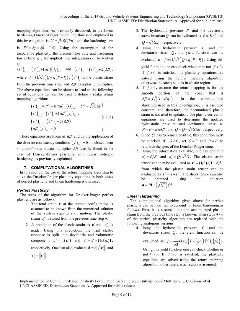
mapping algorithm. As previously discussed, in the linear hardening Drucker-Prager model, the flow rule employed in

this investigation is p f ε σ and the hardening law

is p [14]. Using the assumption of the

associative plasticity, the discrete flow rule and hardening law at time 1nt for implicit time integration can be written

as

11

p p

nn nf

σε ε and

1

p p

n n

,

where 1 3 tf Q P P , p

nε is the plastic strain

from the previous time step, and is a plastic multiplier.

The above equations can be shown to lead to the following set of equations that can be used to define a scalar return mapping algorithm:

1 1

11

1

1

3

0

tr tr

n n

p p

nn n

p p

n n

n

P P K , Q Q G

f ,

f

σε ε

=

(35)

These equations are linear in and by the application of

the discrete consistency condition 10

nf

, a closed form

solution for the plastic multiplier can be found in the

case of Drucker-Prager plasticity with linear isotropic hardening, as previously explained.

7. COMPUTATIONAL ALGORITHMS In this section, the use of the return mapping algorithm to

solve the Drucker-Prager plasticity equations in both cases of perfect plasticity and linear hardening is discussed.

Perfect Plasticity

The steps of the algorithm for Drucker-Prager perfect plasticity are as follows:

1. The total strain ε at the current configuration is assumed to be known from the numerical solution of the system equations of motion. The plastic strain p

nε is stored from the previous time step n.

2. A prediction of the elastic strain as e pn ε ε ε is

made. Using this prediction, the trial elastic response is split into deviatoric and volumetric

components tre ev ε and 1 3e e e

s vε ε I ,

respectively. One can also evaluate e es sn̂ ε ε= and

e es s .

3. The hydrostatic pressure P and the deviatoric stress invariant Q can be evaluated as e

vP K and

6 esQ G , respectively.

4. Using the hydrostatic pressure P and the deviatoric stress Q , the yield function can be

evaluated as 1 3 tf Q P P . Using this

yield function one can check whether or not 0f .

If 0f is satisfied, the plasticity equations are

solved using the return mapping algorithm, otherwise the stress state is in elastic region.

5. If 0f , assume the return mapping is for the

smooth portion of the cone, that is

2f G K . In the computational

algorithm used in this investigation, c is assumed constant, and therefore, the accumulated plastic strain is not used to update c . The plastic correction equations are used to determine the updated hydrostatic pressure and deviatoric stress as

P P K , and 3Q Q G , respectively.

6. Since Q has to remain positive, this condition must

be checked. If 0Q , set 0Q and tP P to

return to the apex of the Drucker-Prager cone. 7. Using the information available, one can compute

ev P K and 6e

s Q G . The elastic strain

tensor can then be evaluated as 1 3e e ev s

ˆ ε I n+ ,

from which the plastic strain tensor can be evaluated as p eε ε ε . The stress tensor can also be obtained using the equation

2 3 ˆP Qσ I n+ .

Linear Hardening

The computational algorithm given above for perfect plasticity can be modified to account for linear hardening as follows. First, it is assumed that the accumulated plastic strain from the previous time step is known. Then steps 4 - 6 of the perfect plasticity algorithm are replaced with the following analogous versions:

4. Using the hydrostatic pressure P and the deviatoric stress Q , the yield function can be

evaluated as 1

3p

nf Q P c .

Using this yield function one can check whether or not 0f . If 0f is satisfied, the plasticity

equations are solved using the return mapping algorithm, otherwise elastic region is assumed.



of 19

5. If 0f , assume the return mapping is for the

smooth portion of the cone, that is

2 2trf G K H . The accumulated

plastic strain is updated using the equation

1

p p

n n

and stored for use in the

next time step. The plastic correction equations are used to determine the updated hydrostatic pressure and deviatoric stress as P P K , and

3Q Q G , respectively.

6. Since Q has to remain positive, this condition must

be checked. If 0Q , set 0Q and

1 1

p

n nP c

to return to the apex of

the Drucker-Prager cone (see Figure 1). In this paper,

2

0p tr p

v nP c H H K

is used to update 01 1

p p

n nc c H

,

where 1

p p pvn n

.

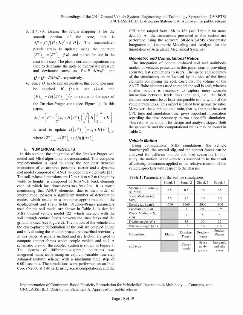
8. NUMERICAL RESULTS

In this section, the integration of the Drucker-Prager soil model and MBS algorithms is demonstrated. This computer implementation is used to study the nonlinear dynamic interaction of an armored personnel carrier and a dynamic soil model composed of ANCF 8-noded brick elements [21]. The soil, whose dimensions are 12 m x 6 m x 2 m (length by width by height), is composed of 36 ANCF brick elements each of which has dimensions1m 2m 2m . It is worth mentioning that ANCF elements, due to their order of interpolation, possess a significant number of deformation modes, which results in a smoother approximation of the displacement and strain fields. Drucker-Prager parameters used for the soil model are shown in Table 1. A detailed MBS tracked vehicle model [22] which interacts with the soil through contact forces between the track links and the ground is used (see Figure 2). The motion of the vehicle and the elasto-plastic deformation of the soil are coupled online and solved using the solution procedure described previously in this paper. A penalty method and dry friction are used to compute contact forces which couple vehicle and soil. A schematic view of the coupled system is shown in Figure 3. The system of differential-algebraic equations was integrated numerically using an explicit, variable time step Adams-Bashforth scheme with a maximum time step of 0.001 seconds. The simulations were performed on an Intel Core i7-2600 at 3.40 GHz using serial computations, and the

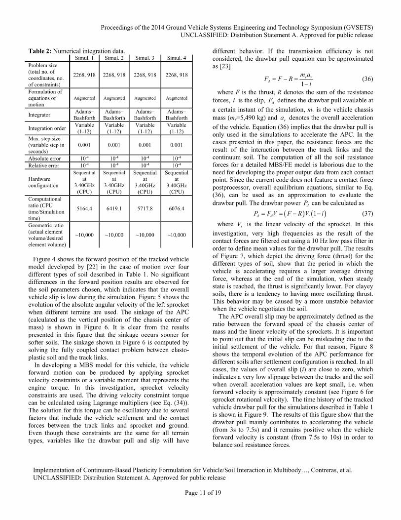
CPU time ranged from 15h to 18h (see Table 2 for more details). All the simulations presented in this section are performed using the software SIGMA/SAMS (Systematic Integration of Geometric Modeling and Analysis for the Simulation of Articulated Mechanical Systems). Geometric and Computational Ratios

The integration of continuum-based soil and multibody models of vehicles presented in this paper aims at providing accurate, fast simulations to users. The speed and accuracy of the simulations are influenced by the size of the finite elements composing the soil. Currently, the volume of the ANCF finite elements used to model the soil is 4m3, whereas smaller volume is necessary to capture more accurate interaction between track links and soil, i.e., the brick element size must be at least comparable to the width of the vehicle track links. This aspect is called here geometric ratio. Moreover, the computational ratio, that is, the ratio between CPU time and simulation time, gives important information regarding the time necessary to run a specific simulation. This ratio is paramount for design and analysis stages. Both the geometric and the computational ratios may be found in Table 2.

Vehicle Motion

Using computational MBS simulations, the vehicle drawbar pull, the overall slip, and the contact forces can be analyzed for different motion and load scenarios. In this study, the motion of the vehicle is assumed to be the result of velocity constraints applied to the relative rotation of the vehicle sprockets with respect to the chassis.

Table 1: Parameters of the soil for simulations. Simul. 1 Simul. 2 Simul. 3 Simul. 4

Modulus of Elasticity (E, MPa)

8.5 8.5 8.5 8.5

Shear Modulus (G, MPa)

3.5 3.5 3.5 3.5

Density (, kg/m3) 1760 1760 2000 1900 Cohesion (c, kPa) 3 0.01 0.75 Plastic Modulus (H, kPa)

5 5 5

Friction angle (,) 35 50 27 Dilatancy angle (,) 1.5 3.5 0.5

Formulation Elastic Drucker-

Prager Drucker-

Prager

Drucker-Prager

Soil type Clayey sands

Dense sandy

gravels

Inorganic and silty

clays



of 19

Table 2: Numerical integration data. Simul. 1 Simul. 2 Simul. 3 Simul. 4 Problem size (total no. of coordinates, no. of constraints)

2268, 918 2268, 918 2268, 918 2268, 918

Formulation of equations of motion

Augmented Augmented Augmented Augmented

Integrator Adams–

Bashforth Adams–

Bashforth Adams–

Bashforth Adams–

Bashforth

Integration order Variable (1-12)

Variable (1-12)

Variable (1-12)

Variable (1-12)

Max. step size (variable step in seconds)

0.001 0.001 0.001 0.001

Absolute error 10-4 10-4 10-4 10-4 Relative error 10-4 10-4 10-4 10-4

Hardware configuration

Sequential at

3.40GHz (CPU)

Sequential at

3.40GHz (CPU)

Sequential at

3.40GHz (CPU)

Sequential at

3.40GHz (CPU)

Computational ratio (CPU time/Simulation time)

5164.4 6419.1 5717.8 6076.4

Geometric ratio (actual element volume/desired element volume)

~10,000 ~10,000 ~10,000 ~10,000

Figure 4 shows the forward position of the tracked vehicle

model developed by [22] in the case of motion over four different types of soil described in Table 1. No significant differences in the forward position results are observed for the soil parameters chosen, which indicates that the overall vehicle slip is low during the simulation. Figure 5 shows the evolution of the absolute angular velocity of the left sprocket when different terrains are used. The sinkage of the APC (calculated as the vertical position of the chassis center of mass) is shown in Figure 6. It is clear from the results presented in this figure that the sinkage occurs sooner for softer soils. The sinkage shown in Figure 6 is computed by solving the fully coupled contact problem between elasto-plastic soil and the track links.

In developing a MBS model for this vehicle, the vehicle forward motion can be produced by applying sprocket velocity constraints or a variable moment that represents the engine torque. In this investigation, sprocket velocity constraints are used. The driving velocity constraint torque can be calculated using Lagrange multipliers (see Eq. (34)). The solution for this torque can be oscillatory due to several factors that include the vehicle settlement and the contact forces between the track links and sprocket and ground. Even though these constraints are the same for all terrain types, variables like the drawbar pull and slip will have

different behavior. If the transmission efficiency is not considered, the drawbar pull equation can be approximated as [23]

1v v

d

m aF F R

i

(36)

where F is the thrust, R denotes the sum of the resistance forces, i is the slip, dF defines the drawbar pull available at

a certain instant of the simulation, mv is the vehicle chassis mass (mv=5,490 kg) and va denotes the overall acceleration

of the vehicle. Equation (36) implies that the drawbar pull is only used in the simulations to accelerate the APC. In the cases presented in this paper, the resistance forces are the result of the interaction between the track links and the continuum soil. The computation of all the soil resistance forces for a detailed MBS/FE model is laborious due to the need for developing the proper output data from each contact point. Since the current code does not feature a contact force postprocessor, overall equilibrium equations, similar to Eq. (36), can be used as an approximation to evaluate the drawbar pull. The drawbar power dP can be calculated as

1d d tP F V F R V i (37)

where tV is the linear velocity of the sprocket. In this

investigation, very high frequencies as the result of the contact forces are filtered out using a 10 Hz low pass filter in order to define mean values for the drawbar pull. The results of Figure 7, which depict the driving force (thrust) for the different types of soil, show that the period in which the vehicle is accelerating requires a larger average driving force, whereas at the end of the simulation, when steady state is reached, the thrust is significantly lower. For clayey soils, there is a tendency to having more oscillating thrust. This behavior may be caused by a more unstable behavior when the vehicle negotiates the soil.

The APC overall slip may be approximately defined as the ratio between the forward speed of the chassis center of mass and the linear velocity of the sprockets. It is important to point out that the initial slip can be misleading due to the initial settlement of the vehicle. For that reason, Figure 8 shows the temporal evolution of the APC performance for different soils after settlement configuration is reached. In all cases, the values of overall slip (i) are close to zero, which indicates a very low slippage between the tracks and the soil when overall acceleration values are kept small, i.e. when forward velocity is approximately constant (see Figure 6 for sprocket rotational velocity). The time history of the tracked vehicle drawbar pull for the simulations described in Table 1 is shown in Figure 9. The results of this figure show that the drawbar pull mainly contributes to accelerating the vehicle (from 3s to 7.5s) and it remains positive when the vehicle forward velocity is constant (from 7.5s to 10s) in order to balance soil resistance forces.



of 19

0 2 4 6 8 10-3

-2

-1

0

1

2

3

4

5F

orw

ard

posi

tion

(m

)

Time (s) Figure 4: Forward position of the chassis center of mass.

( Elastic, Clayey sand, Dense gravels, Silty clays)

0 2 4 6 8 10-5.5

-5.0

-4.5

-4.0

-3.5

-3.0

-2.5

-2.0

-1.5

-1.0

-0.5

0.0

0.5

Spr

ocke

t rot

atio

nal v

eloc

ity

(rad

/s)

Time (s) Figure 5: Sprocket rotational velocity. ( Elastic,

Clayey sand, Dense gravels, Silty clays)

0 2 4 6 8 10-0.02

-0.01

0.00

0.01

0.02

0.03

0.04

Sin

kage

(m

)

Time (s) Figure 6: Sinkage of the chassis center of mass. ( Elastic, Clayey sand, Dense gravels,

Silty clays)

3 4 5 6 7 8 9 10-1

0

1

2

3

4

5

6

7

8

9

10

Thr

ust (

kN)

Time (s) Figure 7: Tracked vehicle thrust. ( Elastic, Clayey sand, Dense gravels, Silty clays)

3 4 5 6 7 8 9 10-3

-2

-1

0

1

2

3

4

5

6

% S

lip

(i)

Time (s) Figure 8: Tracked vehicle slip. ( Elastic, Clayey sand, Dense gravels, Silty clays)

3 4 5 6 7 8 9 10-1

0

1

2

3

4

5

6

7

8

9

Dra

wba

r pu

ll (

kN)

Time (s) Figure 9: Drawbar pull. ( Elastic, Clayey sand,

Dense gravels, Silty clays)



of 19

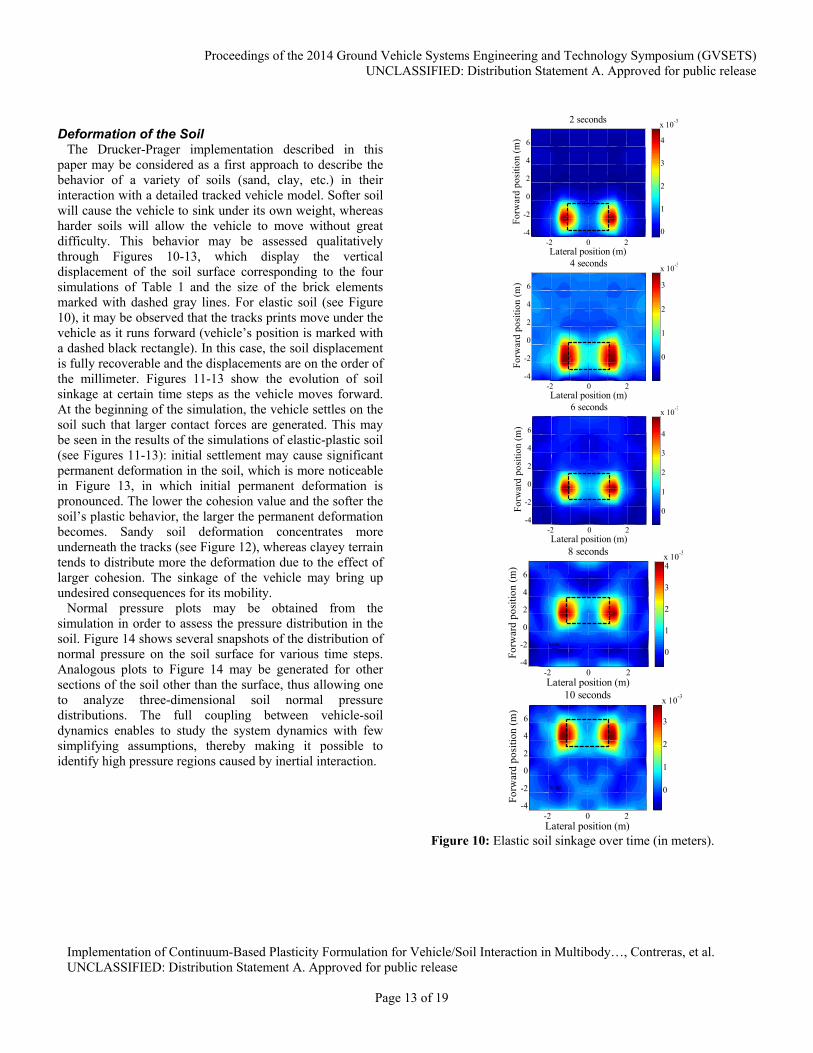
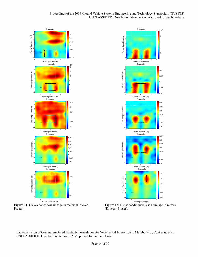
Deformation of the Soil

The Drucker-Prager implementation described in this paper may be considered as a first approach to describe the behavior of a variety of soils (sand, clay, etc.) in their interaction with a detailed tracked vehicle model. Softer soil will cause the vehicle to sink under its own weight, whereas harder soils will allow the vehicle to move without great difficulty. This behavior may be assessed qualitatively through Figures 10-13, which display the vertical displacement of the soil surface corresponding to the four simulations of Table 1 and the size of the brick elements marked with dashed gray lines. For elastic soil (see Figure 10), it may be observed that the tracks prints move under the vehicle as it runs forward (vehicle’s position is marked with a dashed black rectangle). In this case, the soil displacement is fully recoverable and the displacements are on the order of the millimeter. Figures 11-13 show the evolution of soil sinkage at certain time steps as the vehicle moves forward. At the beginning of the simulation, the vehicle settles on the soil such that larger contact forces are generated. This may be seen in the results of the simulations of elastic-plastic soil (see Figures 11-13): initial settlement may cause significant permanent deformation in the soil, which is more noticeable in Figure 13, in which initial permanent deformation is pronounced. The lower the cohesion value and the softer the soil’s plastic behavior, the larger the permanent deformation becomes. Sandy soil deformation concentrates more underneath the tracks (see Figure 12), whereas clayey terrain tends to distribute more the deformation due to the effect of larger cohesion. The sinkage of the vehicle may bring up undesired consequences for its mobility.

Normal pressure plots may be obtained from the simulation in order to assess the pressure distribution in the soil. Figure 14 shows several snapshots of the distribution of normal pressure on the soil surface for various time steps. Analogous plots to Figure 14 may be generated for other sections of the soil other than the surface, thus allowing one to analyze three-dimensional soil normal pressure distributions. The full coupling between vehicle-soil dynamics enables to study the system dynamics with few simplifying assumptions, thereby making it possible to identify high pressure regions caused by inertial interaction.

Lateral position (m)

Forw

ard

posi

tion

(m)

2 seconds

-2 0 2-4

-2

0

2

4

6

0

1

2

3

4

x 10-3


Forw

ard

posi

tion

(m)

4 seconds

-2 0 2-4

-2

0

2

4

6

0

1

2

3

x 10-3


Forw

ard

posi

tion

(m)

6 seconds

-2 0 2-4

-2

0

2

4

6

0

1

2

3

4

x 10-3


Forw

ard

posi

tion

(m)

8 seconds

8.002

-2 0 2-4

-2

0

2

4

6

0

1

2

3

4x 10

-3


Forw

ard

posi

tion

(m)

10 seconds

10.002

-2 0 2-4

-2

0

2

4

6

0

1

2

3

x 10-3

Figure 10: Elastic soil sinkage over time (in meters).



of 19


Forw

ard

posi

tion

(m)

2 seconds

2.002

-3 -2 -1 0 1 2 3-4

-2

0

2

4

6

-0.005

0

0.005

0.01

0.015

0.02

0.025


Forw

ard

posi

tion

(m)

4 seconds

4.002

-2 0 2-4

-2

0

2

4

6

-5

0

5

10

15

20x 10

-3


Forw

ard

posi

tion

(m)

6 seconds

6.002

-3 -2 -1 0 1 2 3-4

-2

0

2

4

6

-0.01

-0.005

0

0.005

0.01

0.015


Forw

ard

posi

tion

(m)

8 seconds

8.002

-3 -2 -1 0 1 2 3-4

-2

0

2

4

6

-0.01

-0.005

0

0.005

0.01

0.015

0.02

0.025


Forw

ard

posi

tion

(m)

10 seconds

10.002

-2 0 2-4

-2

0

2

4

6

-0.01

0

0.01

0.02

Figure 11: Clayey sands soil sinkage in meters (Drucker-Prager).


Forw

ard

posi

tion

(m)

2 seconds

2.002

-3 -2 -1 0 1 2 3-4

-2

0

2

4

6

-5

0

5

10

x 10-3


Forw

ard

posi

tion

(m)

4 seconds

4.002

-3 -2 -1 0 1 2 3-4

-2

0

2

4

6

-0.01

-0.005

0

0.005

0.01


Forw

ard

posi

tion

(m)

6 seconds

6.002

-3 -2 -1 0 1 2 3-4

-2

0

2

4

6

-0.01

-0.005

0

0.005

0.01

0.015

0.02


Forw

ard

posi

tion

(m)

8 seconds

8.002

-3 -2 -1 0 1 2 3-4

-2

0

2

4

6

-0.01

-0.005

0

0.005

0.01

0.015

0.02

0.025


Forw

ard

posi

tion

(m)

10 seconds

10.002

-3 -2 -1 0 1 2 3-4

-2

0

2

4

6

-0.02

-0.01

0

0.01

0.02

0.03

Figure 12: Dense sandy gravels soil sinkage in meters (Drucker-Prager).



of 19


Forw

ard

posi

tion

(m)

2 seconds

2.002

-2 0 2-4

-2

0

2

4

6

-5

0

5

10

15

x 10-3


Forw

ard

posi

tion

(m)

4 seconds

4.002

-3 -2 -1 0 1 2 3-4

-2

0

2

4

6

-5

0

5

10

15

x 10-3


Forw

ard

posi

tion

(m)

6 seconds

6.002

-3 -2 -1 0 1 2 3-4

-2

0

2

4

6

0

5

10

x 10-3


Forw

ard

posi

tion

(m)

8 seconds

8.002

-3 -2 -1 0 1 2 3-4

-2

0

2

4

6

-5

0

5

10

15

20x 10

-3


Forw

ard

posi

tion

(m)

10 seconds

10.002

-3 -2 -1 0 1 2 3-4

-2

0

2

4

6

-0.005

0

0.005

0.01

0.015

0.02

0.025

0.03

Figure 13: Silty clays soil sinkage in meters (Drucker-Prager).


Forw

ard

posi

tion

(m)

2 seconds

-2 0 2-4

-2

0

2

4

6

0

5000

10000

15000


Forw

ard

posi

tion

(m)

4 seconds

-2 0 2-4

-2

0

2

4

6

0

5000

10000

15000


Forw

ard

posi

tion

(m)

6 seconds

-2 0 2-4

-2

0

2

4

6

-5000

0

5000

10000

15000


Forw

ard

posi

tion

(m)

8 seconds

-2 0 2-4

-2

0

2

4

6

-5000

0

5000

10000

15000


Forw

ard

posi

tion

(m)

10 seconds

-2 0 2-4

-2

0

2

4

6

-5000

0

5000

10000

15000

Figure 14: Elastic soil normal pressure on the surface in Pa (positive pressure means compression).



of 19

9. SUMMARY AND CONCLUSIONS In this paper, the formulation and implementation of an

inelastic continuum-based soil model in a general multibody system (MBS) simulation environment is developed. Such a new computational environment will allow for the simulation of the complex and dynamic vehicle-soil interactions. The soil model is developed using ANCF finite elements. A Drucker-Prager plasticity material is used to model the constitutive behavior of the soil. As mentioned in the paper, the Drucker-Prager plasticity models are suitable for the simulation of a number of types of soils and offer a good starting point for computational plasticity in terramechanics applications. Such higher fidelity terramechanics simulations can be fruitfully applied towards the investigation of complex dynamic phenomena in terramechanics. The proposed ANCF/Drucker-Prager soil model is currently being subjected to further testing and improvements in the MBS computer code SIGMA/SAMS. The simulation of higher fidelity soil models and the consideration of flexible track links in the vehicle-soil interaction remain as topics of research for future work. Likewise, there is a need for finer meshes in order to capture the soil pressure produced by each roller in the vehicle. Furthermore, the development of ANCF finite elements specially devised for plasticity formulations and contact interaction is another field of research with a great number of applications in vehicle/soil interaction, which can be exploited in the near future. The simulation of the full coupling between tracked vehicle and soil opens up a range of possibilities for the improvement of design and study of a wide variety of scenarios. Further investigation may also be aimed at refining soil models and more detailed analysis of vehicle performance and soil behavior.

DISCLAIMER Reference herein to any specific commercial products,

process, or service by trade name, trademark, manufacturer, or otherwise, does not necessarily constitute or imply its endorsement, recommendation, or favoring by the United States Government or the Department of the Army (DoA). The views and opinions of authors expressed herein do not necessarily state or reflect those of the United States Government or the DoA, and shall not be used for advertising or product endorsement purposes.

REFERENCES

[1] Contreras, U., Li, G.B., Foster, C.D., Shabana, A.A., Jayakumar, P., and Letherwood, M., 2013, “Soil Models and Vehicle System Dynamics”, Applied Mechanics Reviews, Vol. 65(4), doi:10.1115/1.4024759.

[2] Yakoub, R.Y. and Shabana, A.A., 1999, “Use of Cholesky Coordinates and the Absolute Nodal Coordinate Formulation in the Computer Simulation of Flexible Multibody Systems”, Nonlinear Dynamics, Vol. 20, pp. 267-282.

[3] de Borst, R., and Groen, A.E., 1999, “Towards Efficient and Robust Elements for 3D-Soil Plasticity”, Computers and Structures, Vol. 70, pp. 23-34.

[4] Shoop, S.A., 2001, “Finite Element Modeling of Tire-Terrain Interaction”, U.S. Army Corps of Engineers, Engineer Research and Development Center, Technical Report ERDC/CRREL TR-01-16.

[5] Liu, C.H., and Wong, J.Y., 1996, “Numerical Simulations of Tire-Soil Interaction Based on Critical State Soil Mechanics”, Journal of Terramechanics, 33(5), pp. 209-221.

[6] Xia, K., and Yang, Y., 2012, “Three‐Dimensional Finite Element Modeling of Tire/Ground Interaction”, International Journal for Numerical and Analytical Methods in Geomechanics, 36(4), pp. 498-516.

[7] Hambleton, J.P., and Drescher, A., 2009, “On Modeling a Rolling Wheel in the Presence of Plastic Deformation as a Three-or Two-Dimensional Process”, International Journal of Mechanical Sciences, 51(11), pp. 846-855.

[8] Nankali, N., Namjoo, M., and Maleki, M.R., 2012, “Stress Analysis of Tractor Tire Interaction with Soft Soil using 2D Finite Element Method”, International Journal of Advanced Design and Manufacturing Technology, 5(3), pp. 107-111.

[9] Xia, K., 2011, “Finite element modeling of tire/terrain interaction: Application to Predicting Soil Compaction and Tire Mobility”, Journal of Terramechanics, 48(2), pp. 113-123.

[10] Shoop, S.A., Kestler, K., and Haehnel, R., 2006, “Finite Element Modeling of Tires on Snow”, Tire science and technology, 34(1), pp. 2-37.

[11] Pruiksma, J.P., Kruse, G.A.M.,Teunissen, J.A.M., and van Winnendael, M.F.P., 2011, “Tractive Performance Modelling of the Exomars Rover Wheel Design on Loosely Packed Soil Using the Coupled Eulerian-Lagrangian Finite Element Technique”, 11th Symposium on Advanced Space Technologies in Robotics and Automation, 12-14 April, Noordwijk, The Netherlands.



of 19

[12] Mohsenimanesh, A., Ward, S.M., Owende, P.O.M., and Javadi, A., 2009, “Modelling of Pneumatic Tractor Tyre Interaction with Multi-Layered Soil”, Biosystems Engineering, 104(2), pp. 191-198.

[13] Grujicic, M., Bell, W.C., Arakere, G., and Haque, I., 2009, “Finite Element Analysis of the Effect of Up-Armouring on the Off-Road Braking and Sharp-Turn Performance of a High-Mobility Multi-Purpose Wheeled Vehicle”, Proceedings of the Institution of Mechanical Engineers, Part D: Journal of Automobile Engineering, 223(11), pp. 1419-1434.

[14] de Souza Neto, E.A., Peric, D., and Owen, D.R.J., 2008, Computational Methods for Plasticity: Theory and Applications, Wiley, New York.

[15] Drucker, D.C., and Prager, W., 1952, “Soil Mechanics and Plastic Analysis or Limit Design”, Division of Applied Mathematics, Brown University.

[16] Simo, J.C., and Hughes, T.J.R., 1998, Computational Inelasticity, Springer, New York.

[17] Borja, R.I., 2013, Plasticity: Modeling & Computation, Springer, New York.

[18] Shabana, A.A., 2012, Computational Continuum Mechanics, 2nd ed., Cambridge University Press, Cambridge, UK.

[19] Gerstmayr, J., Sugiyama, H., and Mikkola, A., 2013, “Review on the Absolute Nodal Coordinate Formulation for Large Deformation Analysis of Multibody Systems”, Journal of Computational and Nonlinear Dynamics, 8(3), 031016.

[20] Shabana, A.A., 1998, “Computer Implementation of the Absolute Nodal Coordinate Formulation for Flexible Multibody Dynamics”, Nonlinear Dynamics, Vol. 16, No. 3, pp. 293-306.

[21] Olshevskiy, A., Dmitrochenko, O., and Kim, C.W., 2013, “Three-Dimensional Solid Brick Element Using Slopes in the Absolute Nodal Coordinate Formulation”, ASME Journal of Computational and Nonlinear Dynamics, Vol. 9(2), 021001, doi:10.1115/1.4024910.

[22] Hamed, A.M., Jayakumar, P., Letherwood, M.D., Gorsich, D.J., Recuero, A.M., and Shabana, A.A., 2014, “Ideal Compliant Joints and Integration of Computer Aided Design and Analysis”, ASME Journal of Computational and Nonlinear Dynamics (Accepted for publication)

[23] Wong, J.Y., 2010, Terramechanics and off-road vehicle engineering, 2nd ed., Butterworth - Heinemann, Oxford, UK.

APPENDIX A Perfect Plasticity

It is shown in this appendix that n̂ and fσ can be

evaluated from information obtained from the previous step defined by the subscript n . This result allows reducing the plasticity equations to one linear algebraic equation that can be solved for the consistency parameter which is assumed

to be the same as .

A.1 Yield Function

Using the flow rule p f ε σ and the assumption of

the additive decomposition of the strain e p ε ε ε , the deviatoric elastic strain at the current state can be expressed in terms of the deviatoric elastic strain at the previous step referred to as n as

tre e e e p es s s s s s s sn n

t f σε ε ε ε ε ε ε (A.1)

where tre es s sn

ε ε ε . The yield function can be

written as

2

1

3t tf Q P P J P P (A.2)

It follows that

2

2

2

2

1

2

Jf f Pf : :

J P

J P: :

J

σ σσ σ

σ σσ σ

(A.3)

Using the identities

22

1 1

2 3

J PJ : , ,

S S S I

σ σ (A.4)

where P S σ I is the deviatoric stress tensor, it follows that

2

10

2f : :

J S σ I σ (A.5)

This is a scalar rate equation expressed in terms of the stress tensor rate.

A.2 Stresses

The stress tensor can be written as

3 2

3 2

e ev s

p pv v s s

P K G

K G

σ I S ε ε

ε ε ε ε (A.6)

In this equation, 1 3e ev vε I , where tre e

v ε , and

1 3e e es vε ε I . The deviatoric stress tensor S can be

written as



of 19

2 2p es s sG G S ε ε ε (A.7)

This equation shows that the tensors S and esε are in the

same direction and they vary by a scalar multiplier. Using the preceding equation and the definition of fσ given in Eq.

(A.12) below, one can write

2

2

2 2

ps sn

sn s

tr

G

G G t f

G t

J

σ

S S ε ε

S ε

S S

(A.8)

where the tensor 2trsn

G S S ε . The preceding

equation shows that

2

1 trG t

J

S S (A.9)

It follows that tr,S S , and esε are in the same direction and

e trs

e trs

ˆ εS S

nS ε S

(A.10)

Using the fact that 22 JS and 22tr trJS , one

has

2 2

tr

trJ J

S S (A.11)

Using the Drucker-Prager yield function, one can then write

2 2

3 32 2

tr

tr

ff

J J

σ

S SI I

σ (A.12)

The analysis presented in this appendix shows that n̂ and fσ can be evaluated using the trial state which is based on

results obtained from the previous step. Using Eqs. (A.8) and (A.11), one also has

2 2

1tr tr tr

tr tr

G t G t

J J

S S S S (A.13)

This identity is used in the development presented in this paper.

A.3 Hydrostatic Pressure P

The following equation can be written for the hydrostatic pressure P

3 pv vP K I ε ε = (A.14)

It follows that 1

3 3 pv vn n

P P K K

I I ε ε= + (A.15)

One can define 3trvn

P P KI I ε= + . Using this

definition, Eq. (A.15) can be written as 1

3tr pvn

P P K

I I = (A.16)

Using Eq. (A.12), one has 3: f σI . It follows that

1

tr

nP P K

I I I= , which leads to

1

tr

nP P K

= (A.17)

In this equation, t .

APPENDIX B Linear Hardening

In this appendix, the details of the derivation of the basic equations used to develop the computational algorithm in the case of linear hardening are provided.

B.1 Smooth Portion of Cone

The accumulated plastic strain can be written as p . It follows that p . This leads to

1

p p

n n

(B.1)

The cohesion coefficient can be written as

0p pc c H . It follows that 01 1

p p

n nc c H

which leads to

01

p p

n nc c H

(B.2)

Substituting in the yield function leads to

1

1 1 1

10

3

p

n

n n n

cf Q P

(B.3)

This equation can be written in terms trP and trQ as

1

1

13

3

0

tr

n

p

ntr

f Q G

cP K

(B.4)

which upon the use of Eq. (B.2) leads to

2

1

0

1

3

0

tr tr

n

p

n

f Q G P K

c H H

(B.5)

or

2 2

0

1

3

tr tr

p

n

G K H Q P

c H

(B.6)

This equation can be solved for as



of 19

0

2 2

2 2

1

3

1

3

tr tr p

n

tr tr p

n

Q P c H

G K H

Q P c

G K H

(B.7)

One can show that this equation leads to

2 2 2 2

1

3

p

tr tr n

tr

cQ P

f

G K H G K H

(B.8)

B.2 Apex of Cone

At the apex of the cone, one has p pv , which can

be used to write p pv . It follows that

1

p p pvn n

(B.9)

Using the assumption of linear hardening

0p pc c H , one can write 01 1

p p

n nc c H

which leads to

01

p p pvn n

c c H

(B.10)

Substituting in the yield function leads to

1

1 1 1

10

3

p

n

n n n

cf Q P

(B.11)

Since 1 10p

n nP c

(see Equation (A.16) for

definition of the hydrostatic pressure return mapping formula), one can write

0

2

0 0

p pvn

tr pv

tr p p pv vn

c H

P K

P K c H H

(B.12)

This equation can be written as

2

0p tr p

v nH K P c H

(B.13)

Using this equation, one can solve for pv as

0

2

0

2

2

0

2

tr p

npv

tr p

n

tr p

n

P c H

H K

P c H

H K

P c H

H K

(B.14)

implementation of continuum-based plasticity …gvsets.ndia-mich.org/documents/mstv/2014...such a...

Documents