implementation of control strategies for sterile insect
TRANSCRIPT

HAL Id: hal-01943683https://hal.inria.fr/hal-01943683v2
Submitted on 18 Dec 2020
HAL is a multi-disciplinary open accessarchive for the deposit and dissemination of sci-entific research documents, whether they are pub-lished or not. The documents may come fromteaching and research institutions in France orabroad, or from public or private research centers.
L’archive ouverte pluridisciplinaire HAL, estdestinée au dépôt et à la diffusion de documentsscientifiques de niveau recherche, publiés ou non,émanant des établissements d’enseignement et derecherche français ou étrangers, des laboratoirespublics ou privés.
Implementation of Control Strategies for Sterile InsectTechniques
Pierre-Alexandre Bliman, Daiver Cardona-Salgado, Yves Dumont, OlgaVasilieva
To cite this version:Pierre-Alexandre Bliman, Daiver Cardona-Salgado, Yves Dumont, Olga Vasilieva. Implementationof Control Strategies for Sterile Insect Techniques. Mathematical Biosciences, Elsevier, 2019, 314,pp.43-60. �10.1016/j.mbs.2019.06.002�. �hal-01943683v2�

Implementation of Control Strategies for Sterile InsectTechniques
Pierre-Alexandre Bliman
Sorbonne Universite, Universite Paris-Diderot SPC, Inria, CNRS
Laboratoire Jacques-Louis Lions, equipe Mamba, Paris, France
Daiver Cardona-Salgado
Universidad Autonoma de Occidente, Cali, Colombia
Yves Dumont
CIRAD, Umr AMAP, Pretoria, South Africa
AMAP, Univ Montpellier, CIRAD, CNRS, INRA, IRD, Montpellier, France
University of Pretoria, Department of Mathematics and Applied Mathematics, South Africa
Olga Vasilieva
Universidad del Valle, Cali, Colombia
Abstract
In this paper, we propose a sex-structured entomological model that serves as abasis for design of control strategies relying on releases of sterile male mosquitoes(Aedes spp) and aiming at elimination of the wild vector population in sometarget locality. We consider different types of releases (constant and periodicimpulsive), providing sufficient conditions to reach elimination. However, themain part of the paper is focused on the study of the periodic impulsive con-trol in different situations. When the size of wild mosquito population cannotbe assessed in real time, we propose the so-called open-loop control strategythat relies on periodic impulsive releases of sterile males with constant releasesize. Under this control mode, global convergence towards the mosquito-freeequilibrium is proved on the grounds of sufficient condition that relates the sizeand frequency of releases. If periodic assessments (either synchronized with thereleases or more sparse) of the wild population size are available in real time,we propose the so-called closed-loop control strategy, under which the releasesize is adjusted in accordance with the wild population size estimate. Finally,we propose a mixed control strategy that combines open-loop and closed-loopstrategies. This control mode renders the best result, in terms of overall timeneeded to reach elimination and the number of releases to be effectively carriedout during the whole release campaign, while requiring for a reasonable amountof released sterile insects.
1

Keywords: Sterile Insect Technique, periodic impulsive control, open-loopand closed-loop control, global stability, exponential convergence, saturatedcontrol.
1. Introduction
Since decades, the control of vector-borne diseases has been a major issuein Southern countries. It recently became a major issue in Northern countriestoo. Indeed, the rapid expansion of air travel networks connecting regions ofendemic vector-borne diseases to Northern countries, and the rapid invasion5
and establishment of mosquitoes population, like Aedes albopictus, in Northernhemisphere have amplified the risk of Zika, Dengue, or Chikungunya epidemics1.
For decades, chemical control was the main tool to control or eradicatemosquitoes. Taken into account resistance development and the impact of in-secticides on the biodiversity, other alternatives have been developed, such as10
biological control tools, like the Sterile Insect Technique (SIT).Sterile Insect Technique (SIT) is a promising control method that has been
first studied by E. Knipling and collaborators and first experimented successfullyin the early 1950’s by eradicating screw-worm population in Florida. Since then,SIT has been applied on different pest and disease vectors (see [1] for an overall15
presentation of SIT and its applications).The classical SIT relies on massive releases of males sterilized by ionizing
radiations. However, another technique, called the Wolbachia technique, is un-der consideration. Wolbachia [2] is a symbiotic bacterium that infects manyArthropods, including some mosquito species in nature. These bacteria have20
many particular properties, including one that is very useful for vector control:the cytoplasmic incompatibility (CI) property [3, 4]. CI can be used for twodifferent control strategies:
• Incompatible Insect Technique (IIT): males infected with CI-inducing Wol-bachia produce altered sperms that cannot successfully fertilize uninfected25
eggs. This can result in a progressive reduction of the target population.Thus, IIT can be seen as equivalent to classical SIT.
• Population Replacement (PR): in this case, males and females, infectedwith CI-inducing Wolbachia, are released in a susceptible (uninfected) pop-ulation, such that Wolbachia-infected females will produce more offspring30
∗Corresponding authorEmail addresses: [email protected] (Pierre-Alexandre Bliman),
[email protected] (Daiver Cardona-Salgado), [email protected] (Yves Dumont),[email protected] (Olga Vasilieva)
1See, for instance, the most recent distribution map of Aedes albopictus provided byECDC (European Centre for Disease Prevention and Control, https://ecdc.europa.eu/en/
publications-data/aedes-albopictus-current-known-distribution-june-2018)
Preprint submitted to Elsevier December 18, 2020
than uninfected females. Because Wolbachia is maternally inherited, thiswill result in a population replacement by Wolbachia-infected mosquitoes(such replacements or invasions have been observed in natural popula-tion, see [5] for the example of Californian Culex pipiens). Recent studieshave shown that PR may be very interesting with Aedes aegypti, shorten-35
ing their lifespan (see for instance [6]), or more interesting, cutting downtheir competence for dengue virus transmission [7]. However, it is alsoacknowledged that Wolbachia infection can have fitness costs, so that theintrogression of Wolbachia into the field can fail [6].
Based on these biological properties, classical SIT and IIT (see [8, 9, 10, 11, 12,40
13] and references therein) or population replacement (see [14, 15, 16, 17, 18, 19,20, 6, 21] and references therein) have been modeled and studied theoretically ina large number of papers, in order to derive results to explain the success or fail-ure of these strategies using discrete, continuous or hybrid modeling approaches,temporal and spatio-temporal models. More recently, the theory of monotone45
dynamical systems [22] has been applied efficiently to study SIT [23, 13] orpopulation replacement [24, 25, 26] systems.
In this paper, we derive and study a dynamical system to model the re-lease and elimination process for SIT/IIT. We analyze and compare constantcontinuous/periodic impulsive releases and derive conditions relating the sizes50
and frequency of the releases that are sufficient to ensure successful elimination.Such conditions enable the design of SIT-control strategies with constant orvariable number of sterile males to be released that drive the wild population ofmosquitoes towards elimination. Among all the previous strategies, we are alsoable to derive the best strategy, meaning the one that needs to release the least55
amount of sterile males to reach elimination. This can be of utmost importancefor field applications.
The outline of the paper is as follows. In Section 2, we first develop andbriefly study a simple entomological model that describes the natural evolutionof mosquitoes. Then, in Section 3, we introduce a constant continuous SIT-60
control and determine the size of constant releases that ensures global elimina-tion of wild mosquitoes in the target locality. In Section 4, periodic impulsiveSIT-control with constant impulse amplitude is considered, and a sufficient con-dition relating the size and frequency of periodic releases is derived to ensureglobal convergence towards the mosquito-free equilibrium. This condition en-65
ables the design of open-loop (or feedforward) strategies that ensure mosquitoelimination in finite time and without assessing the size of wild mosquito pop-ulation. Alternatively, Section 5 is focused on the design of closed-loop (orfeedback) SIT-control strategies, which are achievable when periodic measure-ments (either synchronized with releases or more sparse) of the wild population70
size are available in real time. Notice that such estimates may be obtained inpractice e.g. by use of Mark-Release-Recapture (MRR) technique [27]. In suchsituation, the release amplitude is computed on the basis of these measurements.Thorough analysis of the feedback SIT-control implementation mode leads toanother sufficient condition to reach mosquito elimination. This condition re-75
3

lates not only the size and frequency of periodic releases but also the frequencyof sparse measurements. Finally, in Section 6 we propose a mixed control strat-egy for periodic impulsive SIT-control. The latter is essentially based on theuse of the smallest of the release values proposed by the previous open-loop andclosed-loop strategies. It turns out that this control mode renders the best result80
from multiple perspectives: in terms of overall time needed to reach elimina-tion and of peak-value of the input control, but also in terms of total amount ofreleased sterile insects and of number of releases to be effectively carried out dur-ing a whole SIT-control campaign. The paper ends with numerical simulationshighlighting the key features and outcomes of periodic impulsive SIT-control85
strategies (Section 7) followed by discussion and conclusions.
2. A sex-structured entomological model
We consider the following 2-dimensional system to model the dynamics ofmosquito populations. It involves two state variables, the number of males Mand the number of females F .90 {
M = rρFe−β(M+F ) − µMM,
F = (1− r)ρFe−β(M+F ) − µFF.(1a)
(1b)
All the parameters are positive, and listed in Table 1. The model assumesthat all females are equally able to mate. It includes direct and/or indirect com-petition effect at different stages (larvae, pupae, adults), through the parameterβ. The latter may be seen as the ratio, σ
K , between σ, a quantity characterizingthe transition between larvae and adults under density dependence and larvalcompetition, and a carrying capacity K, typically proportional to the breedingsites capacity. The primary sex ratio in offspring is denoted by r ∈ (0, 1), and ρrepresents the mean number of eggs that a single female can deposit in averageper day. Last, µM and µF represent, respectively, the mean death rate of maleand female adult mosquitoes. As a rule, it is observed that in general the malemortality is larger, and we assume throughout the paper that:
µM ≥ µF . (2)
Parameter Description Unitr Primary sex ratio −−ρ Mean number of eggs deposited per female per day day−1
µM , µF Mean death rates for males & females per day day−1
β Characteristic of the competition effect per individual −−
Table 1: Parameters of the sex-structured entomological model (1)
4

Existence and uniqueness of the solutions of the Cauchy problem for dynam-ical system (1) follow from standard theorems, ensuring continuous differentia-bility of the latter with respect to time. System (1) is dissipative: there existsa bounded positively invariant set D with the property that, for any boundedset in E ⊂ R2
+, there exists t∗ = t(D, E) such that(M(0), F (0)
)∈ E implies(
M(t), F (t))∈ D for all t > t∗. The set D is called an absorbing set. In our
case, it may be taken, e.g., as:
D = {(M,F ) : 0 ≤M ≤ C, 0 ≤ F ≤ C} (3)
for some C > 0.
Remark 1. Population models of the form N = B(N)N −µN for several birthrate functions, including B(N) = e−βN , have been studied in [28]. Maturationdelay can also be included [28].
Obviously E∗0 = (0, 0) is a trivial equilibrium of system (1), called themosquito-free equilibrium. Being the state to which one desires to drag thesystem by adequate releases of sterile insects, it will play a central role in thesequel. Denote for future use
NF :=(1− r)ρµF
, NM :=rρ
µM. (4)
These positive constants represent basic offspring numbers related to the wild95
female and male populations, respectively. The first of them governs the numberof equilibria, as stated by the following result, whose proof presents no difficultyand is left to the reader.
Theorem 1 (Equilibria of the entomological model).
• If NF≤1, then system (1) possesses E∗0 as unique equilibrium.100
• If NF > 1, then system (1) also possesses a unique positive equilibriumE∗ := (M∗, F ∗), namely
F ∗ =NF
NF +NM1
βlnNF , M∗ =
NMNF +NM
1
βlnNF .
Notice that the total population at the nonzero equilibrium is given by
M∗ + F ∗ =1
βlnNF . It depends upon the basic offspring number and the
competition parameter β. As an example, mechanical control through reduc-tion of the breeding sites induces an increase of β and consequently a decrease ofthe population at equilibrium. Analogously, altering biological parameters may105
modify the basic offspring number, and therefore the size of the population.The stability of the equilibria is addressed by the following result.
Theorem 2 (Stability properties of the entomological model).
5

• If NF≤1, then the (unique) equilibrium E∗0 is Globally Asymptotically Sta-ble (GAS) for system (1).110
• If NF > 1, then E∗0 is unstable for system (1), and E∗ is GAS in D \{(M, 0),M ∈ R+}.
Figure 1 shows the convergence of all trajectories to the positive equilibriumin the viable case, when NF > 1 (the pertinent case for the applications we havein mind).115
0 M*
0
F*
Figure 1: Phase portrait of model (1) when NF > 1. The positive equilibrium appears at theintersection of the two curves on which F (in red) and M (in blue) vanish.
Proof of Theorem 2.• Assume first NF < 1. Rewriting equation (1b) as follows:
F =(
(1− r)ρe−β(M+F ) − µF)F ≤
((1− r)ρ− µF
)F
one deduces that F < −εF for some positive ε. The state variable F beingnonnegative, it then converges to 0. Using now equation (1a), we deduce thatM converges to 0 too, and the GAS of E∗0 follows.• Assume NF = 1. From equation (1b), F = 0 iff F = 0, otherwise F > 0.
We also derive
F ≤ µF(NF e−βF − 1
)F ≤ µF
(e−βF − 1
)F. (5)
Let 0 < δ. As long as F ≥ δ, then F < −µF(1 − e−βδ
)F and F is (strictly)120
decreasing. When F < δ, using an asymptotic expansion of the right-hand side
6

of (5), we obtain that F ≤ −µFβF 2 +O(F 3), such that 0 is LAS within [0, δ).Altogether, we infer that F converges to 0 and so does M . Thus E∗0 is GASwhen NF = 1.• Assume now that NF > 1. Let us compute the Jacobian matrix related to
entomological system (1), page 4:
J(M,F ) =
−βrρFe−β(M+F ) − µM rρ(1− βF )e−β(M+F )
−β(1− r)ρFe−β(M+F ) (1− r)ρ(1− βF )e−β(M+F ) − µF
.
so that
J(E∗0 ) =
(−µM rρ
0 (1− r)ρ− µF
),
from which we deduce that E∗0 is unstable, as NF > 1.125
For the positive equilibrium E∗, using the fact that e−β(M∗+F∗) =
1
NF, we
have:
J(E∗)
=
−βrρNF
F ∗ − µMrρ
NF(1− βF ∗
)−β(1− r)ρ
NFF ∗ −β(1− r)ρ
NFF ∗
.
Obviously trace{J(E∗)
}< 0 and
det J(E∗)
=β
NF(1− r)ρF ∗
(µM +
rρ
NF
)> 0
so that E∗ is LAS when NF > 1.Using Dulac criterion [29], we now show that system (1) has no closed orbits
wholly contained in the attracting set D defined in (3). Indeed, setting
ψ1(F ) :=1
F, f1(M,F ) := rρFe−β(M+F ) − µMM,
g1(M,F ) := (1− r)ρFe−β(M+F ) − µFF,
let us study the sign of the function
D1(M,F ) :=∂
∂M
(ψ1(F )f1(M,F )
)+
∂
∂F
(ψ1(F )g1(M,F )
).
We have∂
∂M
(ψ1(F )f1(M,F )
)= −βrρe−β(M+F ) − µM
F,
∂
∂F
(ψ1(F )g1(M,F )
)= −β(1− r)ρe−β(M+F ),
and thusD1(M,F ) = −βρe−β(M+F ) − µM
F< 0
7
for all (M,F ) ∈ D such that F > 0. Therefore, Dulac criterion [29] applies,demonstrating that system (1) possesses no nonconstant periodic solutions.Thus, using the fact that E∗ is LAS, by the Poincare-Bendixson theorem, alltrajectories in D \ {(M, 0) : M ≥ 0} converge towards E∗.130
Convergence towards E∗0 clearly occurs in absence of females, i.e. whenF (0) = 0. (Notice that for this reason, the point E∗0 cannot be repulsive.)Consider on the contrary a trajectory such that F (0) > 0. As F ≥ −µFF , thisinduces that F (t) ≥ 0 for any t ≥ 0. We will show that convergence to E∗0 isimpossible, so convergence towards E∗ occurs. First of all, one deduces from(1) and the continuity of F that
M(t) = e−µM tM(0) + rρ
t∫0
e−µM (t−s)F (s)e−β(M(s)+F (s)) ds > 0
for any t > 0. The ratioF
Mis therefore well defined and remains positive along
this trajectory. It is moreover continuously differentiable, and
d
dt
(F
M
)=
F
M
(µM − µF + ρe−β(M+F )
(1− r − r F
M
))> (µM − µF )
F
M
ifF
M≤ 1− r
r. From (2), it is deduced immediately that there exists for this
trajectory a real number T ≥ 0, such that
∀ t ≥ T, F
M>
1− rr
.
Then it holds for any t ≥ T that
F =(
(1− r)ρe−β(M+F ) − µF)F ≥
((1− r)ρe−
β1−rF − µF
)F .
The right-hand side of the previous formula is a continuous function of F whichis positive on (0, 1−rβ lnNF ) and negative on ( 1−r
β lnNF ,+∞). As F (t) > 0 for
any t ≥ 0 (see above), one deduces that
lim inft→+∞
F ≥ 1− rβ
lnNF > 0. (6)
As the compact set D is absorbing, the trajectory is ultimately uniformlybounded. We deduce from this and the uniform bound (6), the existence ofcertain T ′ ≥ T (whose precise value depends upon the considered trajectory)and δ > 0, such that
∀ t ≥ T ′, Fe−βF ≥ δ > 0.
Now, we have for any t ≥ T ′
M ≥ rρδe−βM − µMM,
8

which is strictly positive in a neighborhood of M = 0. The trajectory un-der study therefore stays at a positive distance from the point E∗0 , and, beingconvergent, has to converge to the other equilibrium, namely E∗. This showsthat any trajectory departing with F (0) > 0 converges towards E∗, and finallyconcludes the proof of Theorem 2.135
3. Elimination with constant releases of sterile insects
We now extend system (1), in order to incorporate continuous, constantreleases driven by an equation for MS , the number of sterile males:
M = rρFM
M + γMSe−β(M+F ) − µMM,
F = (1− r)ρ FM
M + γMSe−β(M+F ) − µFF,
MS = Λ− µSMS .
(7a)
(7b)
(7c)
The positive constants µS and γ represent, respectively, the mortality rateof sterile insects, and their relative reproductive efficiency or fitness (comparedto the wild males), which is usually smaller than 1. The nonnegative quantity Λis the number of sterile insects released at the beginning of each release period140
(so that it is a “number of released mosquitoes per time unit”). It is takenconstant over time in the present section. The other parameters are the sameas for model (1), see Table 1.
The mortality of the sterile males is usually larger than that of wild males,so in complement to (2), we also have:
µS ≥ µM . (8)
Assuming t large enough, we may suppose MS(t) at its equilibrium value
M∗S :=Λ
µSin (7c), and the previous system then reduces to
M = rρ
FM
M + γM∗Se−β(M+F ) − µMM,
F = (1− r)ρ FM
M + γM∗Se−β(M+F ) − µFF.
(9a)
(9b)
System (9) is dissipative too, with all trajectories converging towards the sameset D introduced in (3). It admits the same mosquito-free equilibrium E∗0 .145
We are interested here in the issues of existence and stability of positiveequilibria. Driven by the application in view, we assume that the mosquitopopulation is viable (that is NF > 1, see Theorem 1), and focus on conditionssufficient for its elimination.
9

3.1. Existence of positive equilibria150
The mosquito-free equilibrium E∗0 is always an equilibrium of system (9).The following result is concerned with possible supplementary equilibria.
Theorem 3 (Existence of positive equilibria for the SIT entomological modelwith constant releases). Assume NF > 1. Then
• there exists Λcrit > 0 such that system (7) admits two positive distinct155
equilibria if 0 < Λ < Λcrit, one positive equilibrium if Λ = Λcrit, and nopositive equilibrium if Λ > Λcrit;
• the value of Λcrit is uniquely determined by the formula
Λcrit := 2µSβγ
φcrit(NF )
1 + NFNM
, (10)
where φ = φcrit(NF ) is the unique positive solution to the equation
1 + φ
(1 +
√1 +
2
φ
)= NF exp
− 2
1 +
√1 +
2
φ
. (11)
Theorem 3 provides a characterization of the constant release rate abovewhich no positive equilibrium may appear. We prove in the next section (Section3.2) that in such a situation, convergence towards the mosquito-free equilibrium160
E∗0 occurs, which ensures elimination of the wild population.
Proof of Theorem 3.Clearly, nullity of M at equilibrium is equivalent to nullity of F . In order tofind possible nonzero equilibria, let (M∗, F ∗) with M∗ > 0, F ∗ > 0 be one ofthem. The populations at equilibrium have to fulfill:
rρF ∗
M∗ + γM∗Se−β(M
∗+F∗) = µM , (1− r)ρ M∗
M∗ + γM∗Se−β(M
∗+F∗) = µF .
In particular, we have, for NF ,NM defined in (4),
M∗
M∗ + γM∗Se−β(M
∗+F∗) =1
NF,
F ∗
M∗ + γM∗Se−β(M
∗+F∗) =1
NM, (12)
which implies the relation:F ∗
M∗=NFNM
.
Injecting this value in the first equation of (12), the number of males M∗ atequilibrium has to fulfil the equation
M∗
M∗ + γM∗Se−β(1+NFNM
)M∗
=1
NF
10

or again
1 +γM∗SM∗
= NF e−β(1+NFNM
)M∗
. (13)
The study of equation (13) is done through the following result, whose proof isgiven in Appendix.
Lemma 1. Let NF > 1, then equation (11) admits a unique positive root,denoted φcrit. Moreover, for any a, c positive, the equation
f(x) := 1 +a
x−NF e−cx = 0 (14)
admits two positive distinct roots if 0 < ac < 2φcrit; one positive root if ac =165
2φcrit; no positive root otherwise.
Using Lemma 1 with the two positive constants
a := γM∗S = γΛ
µS, c := β
(1 +NFNM
),
one deduces that equation (13) admits exactly one positive root when the root
of (11) is equal to φcrit = ac2 = 1
2βγ(
1 + NFNM
) Λcrit
µS, which implies (10) and
thus achieves the proof of Theorem 3.
3.2. Asymptotic stability of the equilibria170
Assume NF > 1. We first study the asymptotic stability of the mosquito-free equilibrium E∗0 in the case where it is the unique equilibrium, that is whenΛ > Λcrit.
Theorem 4 (Stability of the mosquito-free equilibrium of the SIT entomologicalmodel with constant releases). If system (7) admits no positive equilibrium (that175
is, if Λ > Λcrit), then the mosquito-free equilibrium E∗0 is globally exponentiallystable.
Proof of Theorem 4. The Jacobian matrix J(M,F ) of the reduced system (9)is defined by its four coefficients
J21 :=(1− r)ρFM + γM∗S
e−β(M+F )
(1− βM − M
M + γM∗S
), J11 :=
r
1− rJ21 − µM ,
J12 :=rρM
M + γM∗Se−β(M+F )(1− βF ), J22 :=
1− rr
J12 − µF .
Its value at the mosquito-free equilibrium E∗0 is just diag{−µM ;−µF }, whichguarantees local asymptotic stability at this point.
11
We use again Dulac criterion to show that system (9) has no closed orbitswholly contained in the set D. We set
ψ2(M,F ) :=M + γM∗SMF
,
f2(M,F ) := rρFM
M + γM∗Se−β(M+F ) − µMM,
g2(M,F ) := (1− r)ρ FM
M + γM∗Se−β(M+F ) − µFF,
and then study the sign of the function
D2(M,F ) :=∂
∂M
(ψ2(M,F )f2(M,F )
)+
∂
∂F
(ψ2(M,F )g2(M,F )
).
As∂
∂M
(ψ2(M,F )f2(M,F )
)= −βrρe−β(M+F ) − µM
F,
∂
∂F
(ψ2(M,F )g2(M,F )
)= −β(1− r)ρe−β(M+F ),
one hasD2(M,F ) = −βρe−β(M+F ) − µM
F< 0,
for all (M,F ) ∈ D such that F > 0. Thus, by the Poincare-Bendixson theorem,180
since E∗0 is the only asymptotically stable equilibrium, all trajectories in Dapproach the equilibrium E∗0 . This concludes the proof of Theorem 4.
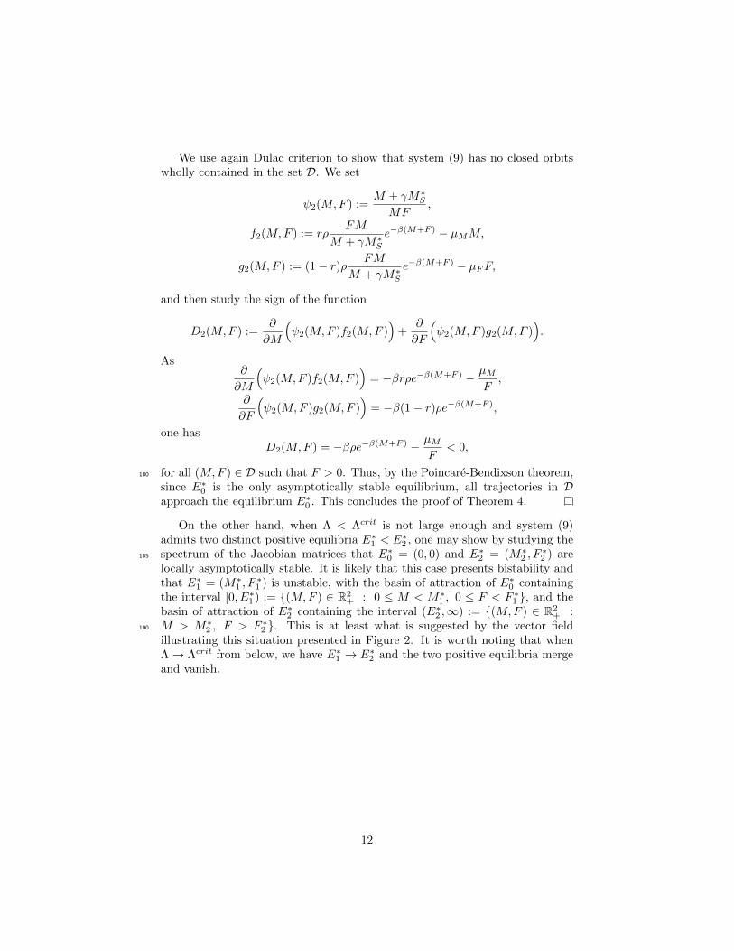
On the other hand, when Λ < Λcrit is not large enough and system (9)admits two distinct positive equilibria E∗1 < E∗2 , one may show by studying thespectrum of the Jacobian matrices that E∗0 = (0, 0) and E∗2 = (M∗2 , F
∗2 ) are185
locally asymptotically stable. It is likely that this case presents bistability andthat E∗1 = (M∗1 , F
∗1 ) is unstable, with the basin of attraction of E∗0 containing
the interval [0, E∗1 ) := {(M,F ) ∈ R2+ : 0 ≤ M < M∗1 , 0 ≤ F < F ∗1 }, and the
basin of attraction of E∗2 containing the interval (E∗2 ,∞) := {(M,F ) ∈ R2+ :
M > M∗2 , F > F ∗2 }. This is at least what is suggested by the vector field190
illustrating this situation presented in Figure 2. It is worth noting that whenΛ→ Λcrit from below, we have E∗1 → E∗2 and the two positive equilibria mergeand vanish.
12
0 M*
M1*
M2*
0
F*
F1*
F2*
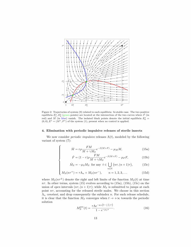
Figure 2: Trajectories of system (9) related to each equilibria: bi-stable case. The two positiveequilibria E∗
1 , E∗2 (green points) are located at the intersection of the two curves where F (in
red) and M (in blue) vanish. The isolated black points denote the initial equilibria E∗0 =
(0, 0), E∗ = (M∗, F ∗) of the system (1), present when no control is applied.
4. Elimination with periodic impulsive releases of sterile insects
We now consider periodic impulsive releases Λ(t), modeled by the followingvariant of system (7):
M = rρFM
M + γMSe−β(M+F ) − µMM,
F = (1− r)ρ FM
M + γMSe−β(M+F ) − µFF,
MS = −µSMS for any t ∈⋃n∈N
(nτ, (n+ 1)τ
),
MS(nτ+) = τΛn +MS(nτ−), n = 1, 2, 3, . . .
(15a)
(15b)
(15c)
(15d)
where MS(nτ±) denote the right and left limits of the function MS(t) at timenτ . In other terms, system (15) evolves according to (15a), (15b), (15c) on theunion of open intervals (nτ, (n+ 1)τ); while MS is submitted to jumps at eachpoint nτ , accounting for the released sterile males. We choose in this sectionΛn constant, and drop consequently the subindex n. For such release schedule,it is clear that the function MS converges when t → +∞ towards the periodicsolution
MperS (t) =
τΛe−µS(t−b tτ cτ)
1− e−µSτ. (16)
13

We therefore introduce now the following periodic system:M = rρ
FM
M + γMperS (t)
e−β(M+F ) − µMM,
F = (1− r)ρ FM
M + γMperS (t)
e−β(M+F ) − µFF.
(17a)
(17b)
Existence and uniqueness of continuously differentiable solutions of system (17)on the interval [0,+∞) may be shown by standard arguments, as well as theforward invariance of the positive orthant. Notice that the mosquito-free equilib-rium E∗0 previously introduced is still an equilibrium of (17). We are interestedhere in studying the conditions under which E∗0 is globally asymptotically sta-ble. For future use, we note that the mean value of 1/Mper
S corresponding to(16) verifies:⟨
1
MperS
⟩:=
1
τ
∫ τ
0
1
MperS (t)
dt =1− e−µSτ
τ2Λ
∫ τ
0
eµStdt =2(
cosh (µSτ)− 1)
µSτ2Λ.
(18)
Theorem 5 (Sufficient condition for elimination by periodic impulses). For anygiven τ > 0, assume that Λ is chosen such that
Λ ≥ Λcritper
:=cosh (µSτ)− 1
µSτ21
eβγmin
{2NM , 2NF ,max{r, 1− r}max
{NMr,NF
1− r
}}.(19)
Then every solution of system (17) converges globally exponentially to the mosquito-195
free equilibrium E∗0 .
Notice that in (19) and in the sequel, e = e1. The previous result providesa simple sufficient condition for stabilization of the mosquito-free equilibrium,through an adequate choice of the amplitude of the releases, Λ, for given periodτ .200
Remark 2. When r = 1−r and NF > NM (which is the case of the applicationwe are interested in), the expression of Λcritper simplifies as follows:
Λcritper =2(
cosh (µSτ)− 1)
µSτ2NFeβγ
.
The function τ 7→ 2 cosh (µSτ)− 1
µSτ2is increasing and tends towards µS when
τ → 0. Making τ → 0+, we derive the following sufficient condition for stabi-lization:
Λcritper ≥µSNFeβγ
,
to be compared to Λcrit = 2µSβγ
φcrit(NF )
1+NFNM
(see Theorem 3).
14

Proof of Theorem 5. First rewrite (17) as
M =
(rρ
F
M + γMperS
e−β(M+F ) − µM)M,
F =
((1− r)ρ M
M + γMperS
e−β(M+F ) − µF)F,
(20a)
(20b)
in order to emphasize the factorization of M and F .
• 1. Notice that, for any M,F ≥ 0 and any t ≥ 0,
M
M + γMperS
e−β(M+F ) ≤ M
M + γMperS
e−βM ≤ α
M + γMperS
≤ α
γMperS
,
(21)
where we write for simplicity
α := max{xe−βx : x ≥ 0
}=
1
eβ. (22)
Integrating (20b) between nτ and t > nτ leads to
F(t)≤ e
∫ t
nτ
((1− r)ρ M
M + γMperS
e−β(M+F ) − µF)dsF (nτ)
≤ e
∫ t
nτ
((1− r)ρα
γ
1
MperS (s)
− µF)dsF (nτ).
Thus, taking t = (n+ 1)τ , for any n ∈ N, we deduce that
F((n+ 1)τ
)≤ e
((1−r)ρ
α
γ
⟨1
MperS
⟩−µF
)τ
F (nτ).
Therefore, the sequence{F (nτ)
}n∈N decreases towards 0, provided that
(1− r)ραγ
⟨1
MperS
⟩< µF ,
that is ⟨1
MperS
⟩<γ
α
µF(1− r)ρ
= eβγ1
NF, (23)
This is sufficient to ensure that F converges towards 0, and this induces thesame behavior for M : condition (23) implies that E∗0 is GAS.205
• 2. The same argument may be conducted from (20a) rather than (20b), leadingto:
F
M + γMperS
e−β(M+F ) ≤ F
M + γMperS
e−βF ≤ α
M + γMperS
≤ α
γMperS
(24)
15
Global asymptotic stability is thereby guaranteed if⟨1
MperS
⟩<γ
α
µMrρ
= eβγ1
NM. (25)
• 3. Define the positive definite function
V(M,F ) :=1
2(M2 + F 2) (26)
and write its derivative along the trajectories of (17) as
V = MM + FF = −µMM2 − µFF 2 + ρFM(rM + (1− r)F )
M + γMperS
e−β(M+F ). (27)
On the one hand, we have
−µMM2 − µFF 2 ≤ −min{µM , µF }(M2 + F 2) = −2 min{µM , µF }V.
On the other hand,
FM(rM + (1− r)F )
M + γMperS
e−β(M+F ) ≤ max{r, 1− r}FM(M + F )
M + γMperS
e−β(M+F )
≤ max{r, 1− r}α FM
M + γMperS
≤ max{r, 1− r}α 1
M + γMperS
V
≤ max{r, 1− r}α 1
γMperS
V.
Coming back to (27), we deduce that
V ≤(
max{r, 1− r}α 1
γMperS
− 2 min{µM , µF })V.
One may conclude that E∗0 is GAS provided that
max{r, 1− r}ραγ
⟨1
MperS
⟩< 2 min{µM , µF },
that is,⟨1
MperS
⟩< 2
γ
α
min{µM , µF }max{r, 1− r}ρ
= 2eβγ1
max{r, 1− r}min
{r
NM,
1− rNF
}.
(28)
16
• 4. Finally, putting together the sufficient conditions in (23), (25) and (28)yields the following sufficient condition for global asymptotic stability of E∗0 :210 ⟨
1
MperS
⟩< eβγmax
{1
NM,
1
NF,
2
max{r, 1− r}min
{r
NM,
1− rNF
}}.
Expressing the mean value as a function of Λ with the help of (18), oneestablishes that E∗0 is GAS if
Λ >2
eβγ
cosh(µSτ)− 1
µSτ21
max{
1NM ,
1NF ,
2max{r,1−r} min
{rNM ,
1−rNF
}}=
2
eβγ
cosh(µSτ)− 1
µSτ2min
NM ,NF , max{r, 1− r}
2 min{
rNM ,
1−rNF
}
=2
eβγ
cosh(µSτ)− 1
µSτ2min
{NM ,NF ,
max{r, 1− r}2
max
{NMr,NF
1− r
}},
which is exactly the formula (19). This concludes the proof of Theorem 5.
Remark 3. A rough upper bound estimate for Λcritper can be obtained using theresult from the constant continuous release case: if Λ is chosen such that Λ >
Λcrit := 2µSβγ
φcrit(NF )
1 + NFNM
, then E∗0 is GAS for the constant continuous release
system (7). Thus, using a comparison principle, a sufficient condition to ensureglobal asymptotic stability of E∗0 is to choose
MperS ≥ Λcrit
µS,
where MperS = min
t∈[0,τ ]MperS (t) = τΛ
e−µSτ
1− e−µSτ. Thus, we derive that, for a given
τ , if
Λ ≥ ΛcriteµSτ − 1
µSτ, (29)
then E∗0 is GAS. When τ → 0+, we recover the result for the constant continuousrelease (cf. Theorem 3).215
5. Elimination by feedback control
We now assume that measurements are available, providing real time es-timates of the number of wild males and females M(t), F (t), at least for anyt = nτ, n ∈ N. One thus has the possibility to choose the number τΛn ofmosquitoes released at time nτ in view of this information: this is a closed-loop220
control option. We study in the sequel this strategy.
17

5.1. Principle of the method
The principle of the stabilization method that we introduce now is basedon two steps. The first one (Section 5.1.1) consists in solving the stabilizationproblem under the hypothesis that one can directly actuate on MS . The second225
one (Section 5.1.2) consists in showing how to realize, through adequate choiceof Λn, the prescribed behavior of MS defined in Step 1. The formal statementand proof are provided later, in Section 5.2.
5.1.1. Step 1 – Setting directly the sterile population level
We first suppose to be capable of directly controlling the quantity MS . We230
will rely on the following key property.
Proposition 1. Let k be a real number such that
0 < k <1
NF. (30)
Then every solution of (7a)-(7b) such that
M(t)
M(t) + γMS(t)≤ k, t ≥ 0 , (31)
converges exponentially to E∗0 .
The idea behind formula (30) is quite natural: it suffices to impose a fixed
upper bound k on the ratioM
M + γM∗Sin order to make the ‘apparent’ basic
offspring number kNF smaller than 1, and consequently to render inviable the235
wild population. Notice that this condition corresponds exactly to the stabilityof the system linearized around the origin. It may be excessively demanding forlarge population sizes, as it ignores the effects of competition modeled by theexponential term. We shall come back to this point in Section 6 and introducesaturation.240
Proof of Proposition 1. From equations (7a) and (7b), we have, for any solutionthat fulfils (31):
M = rρFM
M + γMSe−β(M+F ) − µMM
≤ rρ FM
M + γMS− µMM ≤ −µMM + rρkF (32a)
and
F = (1− r)ρ FM
M + γMSe−β(M+F ) − µFF ≤ ((1− r)ρk − µF )F. (32b)
The linear autonomous system(M ′
F ′
)=
(−µM rρk
0 −µF + (1− r)ρk
)(M ′
F ′
)(33)
18

is monotone [22] (it involves a Metzler matrix) and may thus serve as a com-parison system for the evolution of (7a)-(7b). Thus, it is deduced that
0 ≤M(t) ≤M ′(t), 0 ≤ F (t) ≤ F ′(t), t ≥ 0,
where (M ′, F ′) is the solution of (33) generated by the same initial values asthe underlying solution (M,F ) of (7a)-(7b).
On the other hand, system (33) is asymptotically stable when (30) holds. Inother words, M ′(t) and F ′(t) converge to E∗0 asymptotically. In consequence,M(t) and F (t) also converge to E∗0 asymptotically when (30) is in force. This245
achieves the proof of Proposition 1.
5.1.2. Step 2 – Shaping an impulsive control compliant with Step 1
We now want to ensure that condition (31) is fulfilled, through an adequatechoice of the impulse amplitude Λn. In virtue of (15c)-(15d), the value of MS
on the interval(nτ, (n+ 1)τ
]is given by
MS(t) = MS(nτ+)e−µS(t−nτ) =(Λnτ +MS(nτ)
)e−µS(t−nτ), (34)
and we would like to choose Λn in such a way that (31) stays in force. However,instead of computing the (nonlinear) evolution of M(t) on the interval
(nτ, (n+
1)τ], we will impose, rather than (31), the stronger condition
γMS(t) ≥(
1
k− 1
)M ′(t), t ≥ 0 (35)
where M ′(t) refers to the super-solution of M(t) introduced in the proof ofProposition 1. (Notice that the conservatism introduced in this step remainsreasonable when the original nonlinear system evolves in region where β(M +250
F )� 1.) Due to its linearity, system (33) may be solved explicitly on(nτ, (n+
1)τ]
using the following result.
Lemma 2. The solution of system (33) on(nτ, (n + 1)τ
]with initial values(
M ′(nτ), F ′(nτ))
=(M(nτ), F (nτ)
)is given by(
M ′(t)F ′(t)
)= P
(M(nτ)F (nτ)
)(36a)
where
P :=
e−µM (t−nτ) rρk
µM − µF + (1− r)ρk(e−(µF−(1−r)ρk)(t−nτ) − e−µM (t−nτ))
0 e−(µF−(1−r)ρk)(t−nτ)
(36b)
19

The proof of Lemma 2 presents no difficulty and is left to the reader.All the components of the matrix in (36a) are nonnegative provided that µF ,255
µM , ρ and k are chosen such that µF − µM − (1− r)ρk ≤ 0. It is worthwhile torecall that µF ≤ µM (see (2), page 4); therefore, the former condition is indeedverified for any positive ρ and k.
We now come back to the control synthesis. Using (34) and (36a), condition(35) is equivalent, on any interval
(nτ, (n+ 1)τ
], with the condition260
γ(Λnτ +MS(nτ)
)e−µS(t−nτ) = γMS(t) ≥
(1
k− 1
)M ′(t)
=1− kk
(e−µM (t−nτ)M(nτ)
+rρk
µM − µF + (1− r)ρk
(e−(µF−(1−r)ρk)(t−nτ) − e−µM (t−nτ)
)F (nτ)
).(37)
This condition is equivalent to
Λnτ ≥ −MS(nτ) +1− kγk
e(µS−µM )s(M(nτ)
+rρk
µM − µF + (1− r)ρk
(e(µM−µF+(1−r)ρk)s − 1
)F (nτ)
)(38)
for any s ∈ [0, τ ]. In virtue of the relationships (2) and (8), the right-hand sideof previous inequality (38) is increasing in s. Therefore, condition (38) has tobe checked only for s = τ .
5.2. Stabilization result
5.2.1. Synchronized measurements and releases265
We now state and prove the stabilization result suggested by the previousconsiderations.
Theorem 6 (Sufficient condition for stabilization by impulsive feedback con-
trol). For a given k ∈(
0, 1NF
), assume that for any n ∈ N:
τΛn ≥∣∣∣∣K (M(nτ)
F (nτ)
)−MS(nτ)
∣∣∣∣+
K :=1
γ
(1−kk e(µS−µM )τ
rρ(1−k)µM−µF+(1−r)ρk
(e(µS−µF+(1−r)ρk)τ − e(µS−µM )τ
))T
(39a)
(39b)
Then every solution of system (15) converges exponentially towards E∗0 , witha convergence rate bounded from below by a value independent of the initialcondition.270
If moreover
τΛn ≤ K
(M(nτ)F (nτ)
)(39c)
then the series of impulses+∞∑n=0
Λn converges.
20

In (39a), the notation |z|+ := max{0, z} represents the positive part of thereal number z. Notice that the row vector K defined in (39b) has positivecomponents.
Implementing the previous control law necessitates the measurement ofM(nτ),F (nτ) (or their upper estimates), and of MS(t) (or its lower estimate). A possi-bility to have (39a) fulfilled, is to ignore the population of sterile males alreadypresent at time nτ and to take simply the linear control law
τΛn = K
(M(nτ)F (nτ)
).
Notice that this expression corresponds to the value in the right-hand side of275
(39c).On the other hand, (39a) means that the release of sterile males at time
t = nτ is not (really) necessary if the sterile males population is large enough,
more precisely if MS(nτ) ≥ K
(M(nτ)F (nτ)
). Using this result, one may avoid
unnecessary releases, thereby reducing the overall cumulative number of released280
males and the underlying cost of SIT control.
Proof of Theorem 6. When(M(nτ), F (nτ)
)= (0, 0), an impulsion Λn has no
effect on the evolution of (M,F ): the origin is an equilibrium point of system(15). We now consider the case
(M(nτ), F (nτ)
)6= (0, 0).
• 1. Assume first that (39a) is fulfilled with a strict inequality. By construction,one has:
∀ t ∈(nτ, (n+ 1)τ
], γMS(t) >
1− kk
M ′(t) (40)
where (M ′, F ′) stands for solution of (33) departing from(M(nτ), F (nτ)
)at285
time nτ .We will first establish that this implies:
∀ t ∈[nτ, (n+ 1)τ
], M(t) ≤M ′(t), F (t) ≤ F ′(t). (41)
For this, let t0 be any element of[nτ, (n + 1)τ
)such that M(t0) ≤ M ′(t0),
F (t0) ≤ F ′(t0) with at least one equality. Let us show the existence of t1 suchthat t0 < t1 < (n+ 1)τ and
∀ t ∈ (t0, t1), M(t) < M ′(t), F (t) < F ′(t). (42)
Indeed, due to (40) and by definition of t0, one has
γMS(t0) >1− kk
M ′(t0) ≥ 1− kk
M(t0),
where we write by convention MS(t0) := MS(nτ+) when t0 = nτ . By continuityof the functions M(t) and MS(t) on the open interval
(nτ, (n+ 1)τ
), there thus
exists t1 such that t0 < t1 < (n+ 1)τ and
∀ t ∈ (t0, t1), γMS(t) >1− kk
M(t).
21
In such conditions, it can be shown as in Proposition 1 that(M ′(t), F ′(t)
)≥(
M(t), F (t))
for any t ∈ (t0, t1), and even that(M ′(t), F ′(t)
)>(M(t), F (t)
),
because the functions defining the right-hand sides of (15a) and (15b) take onstrictly smaller values than those defining the right-hand sides of (33). There-290
fore, for any t0 ∈{nτ+
}∪(nτ, (n + 1)τ
), there exists t1 > t0 such that (42)
holds.From (42) and the fact that
(M(nτ), F (nτ)
)=(M ′(nτ), F ′(nτ)
), one de-
duces that (42) is true for t1 = (n+1)τ , and therefore that (41) is true. Finally,putting together (40) and (41) yields the following key property:
∀ t ∈(nτ, (n+ 1)τ
], γMS(t) >
1− kk
M(t). (43)
• 2. Assume now that (39a) is fulfilled (with the original non-strict inequality).Considering values of Λn converging from above towards the quantity in theright-hand side of this inequality and relying on the continuity of the flow withrespect to Λn, yields instead of (43) the non-strict inequality:
∀t ∈ (nτ, (n+ 1)τ ], γMS(t) ≥ 1− kk
M(t). (44)
• 3. Let us now study F . In view of (44), we have that for any t ∈(nτ, (n+1)τ
]it holds that
M(t)
M(t) + γMS(t)e−β(M(t)+F (t)) ≤ M(t)
M(t) + γMS(t)≤ k.
Therefore,
F = (1− r)ρ FM
M + γMSe−β(M+F ) − µFF ≤
((1− r)ρk − µF
)F.
Due to (39b), there exists ε > 0 such that
µF − (1− r)ρk > ε
and then F ≤ −εF . This property ensures that F (t) decreases with time, and295
converges exponentially towards 0. It is then deduced from (15a) that M(t) alsoconverges exponentially towards 0: overall,
(M(t), F (t)
)converges towards E∗0 .
• 4. Last, choose now Λn fulfilling (39a) and (39c). From the property ofexponential stability previously demonstrated, there exist C, ε > 0 such that300
22

M(t) < Ce−εt and F (t) < Ce−εt for any t ≥ 0. We then deduce that
Λn ≤ 1
γτ
(1− kk
e(µS−µM )τM(nτ)
+rρ(1− k)
µM − µF + (1− r)ρk
(e(µS−µF+(1−r)ρk)τ − e(µS−µM )τ
)F (nτ)
)≤ C
γτ
(1− kk
e(µS−µM )τ
+rρ(1− k)
µM − µF + (1− r)ρk
(e(µS−µF+(1−r)ρk)τ − e(µS−µM )τ
))e−nετ ,
and one gets by summation
+∞∑n=0
Λn ≤C
γτ
(1− kk
e(µS−µM )τ
+rρ(1− k)
µM − µF + (1− r)ρk
(e(µS−µF+(1−r)ρk)τ − e(µS−µM )τ
)) 1
1− e−ετ.
This shows the convergence of the series and concludes the proof of Theorem 6.
5.2.2. Sparse measurements
The feedback control approach requires to assess the size of mosquito pop-305
ulation at every time t ∈ τN. As mentioned in the Introduction, rough esti-mates of a wild population are achievable through direct capture and counting,or through more sophisticated methods such as Mark-Release-Recapture [27].However, this protocol is long and costly. We now show how it is possible toreduce its frequency and to complete measurements only with a period pτ for310
some p ∈ N∗ := N \ {0}. The values of the (p − 1) intermediate releases arecomputed using the last sampled information.
The following result adapts in consequence the control laws given in Theorem6 to sparse measurements.
Theorem 7 (Stabilization by impulsive control with sparse measurements). Let
p ∈ N∗. For a given k ∈(
0, 1NF
), assume for any n ∈ N, m = 0, 1, . . . , p− 1,
τΛnp+m ≥
∣∣∣∣∣Kp
(M(nτ)F (nτ)
)−MS(npτ)e−mµSτ −
m−1∑i=0
Λnp+ie−µS(m−i)τ
∣∣∣∣∣+
Kp :=eµSτ
γ
(1−kk e−(m+1)µMτ
rρ(1−k)µM−µF+(1−r)ρk
(e−(µF−(1−r)ρk)(m+1)τ − e−µM (m+1)τ
))T
(45a)
(45b)
Then every solution of system (15) converges exponentially towards E∗0 , with315
a convergence speed bounded from below by a value independent of the initialcondition.
23

If moreover
τΛnp+m ≤ Kp
(M(nτ)F (nτ)
), (45c)
then the series of impulses+∞∑n=0
Λn converges.
Notice that Theorem 7 represents an extension of Theorem 6, recovered inthe case p = 1 (and thus m = 0): in this case, (45a) boils down to (39a).320
Proof of Theorem 7. The demonstration comes from a slight adaptation of theproof of Theorem 6. Indeed, it suffices to verify that, under the conditions inTheorem 7, property (37) holds on the interval (npτ, (n + 1)pτ ], of length pτ .Let m ∈ {0, 1, . . . , p− 1}. One has for any s ∈ (0, τ ] that
MS
(s+ (np+m)τ
)=(
Λnp+mτ +MS
((np+m)τ
))e−µSs
=(
Λnp+mτ + Λnp+m−1τe−µSτ + . . .
+ Λnpτe−mµSτ +MS(npτ)e−mµSτ
)e−µSs.
Inequality (37) is thus true on((np + m)τ, (np + m + 1)τ
]if and only if it
is imposed that, for any m ∈ {0, 1, . . . , p − 1} and any s ∈ (0, τ ], γ(
Λnp+mτ +
Λnp+m−1τe−µSτ+· · ·+Λnpτe
−mµSτ+MS(npτ)e−mµSτ)e−µSs ≥ 1−k
k
(e−µM (s+mτ)
M(nτ) + rρkµM−µF+(1−r)ρk
(e−(µF−(1−r)ρk)(s+mτ) − e−µM (s+mτ)
)F (nτ)
), that is,
Λnp+mτemµSτ + Λnp+m−1τe
(m−1)µSτ + · · ·+ Λnpτ +MS(npτ)
≥ 1− kγk
(e(µS−µM )(s+mτ)M(nτ)
+rρk
µM−µF + (1−r)ρk
(e(µS−µF+(1−r)ρk)(s+mτ)−e(µS−µM )(s+mτ)
)F (nτ)
)(46)
In virtue of the relationships (2) and (8), the right-hand side of (46) is an325
increasing function of s. Therefore, (46) is more restrictive when taken at s = τ .This yields (45a) and shows the first part of the result. The convergence of theseries of impulses is demonstrated similarly to Theorem 6.
6. Mixed impulsive control strategies
The results obtained in the previous sections for open-loop and closed-loop330
SIT control allow us to compare several SIT release strategies. Here, we consideronly periodic impulsive control, which is more realistic than continuous control.
The open-loop approach (developed in Section 4), is based on the determi-nation of a sufficient size of sterile males to be released, in order to eradicate thewild population. This choice is made according to (19). Under this approach,335
24

even though the previous formula is ‘tight’, the same amount of sterile insectsis used during the whole release campaign.
On the contrary, the closed-loop control approach (exposed in Section 5)is based on estimates of the wild population and thereby it enables fitting therelease sizes. As evidenced by (39a), under this approach the released volume340
is essentially chosen as proportional to the measured population. However, thiscondition is certainly too demanding for large values of M,F (see the commentspreceding Lemma 2). Taking advantage of the apparent complementarity of thetwo approaches, we propose here mixed impulsive control strategies, combiningthe two previous modes. They gather the advantages of both approaches, guar-345
anteeing convergence to the mosquito-free equilibrium with releases that remainbounded (like the periodic impulsive control strategies, Section 4) and vanishingwith the wild population (like the feedback control strategies, Section 5).
Theorem 8. Let p ∈ N∗. Assume that, for any n ∈ N, Λn is chosen at leastequal to the smallest of the right-hand side of (45a) and of a positive constant350
Λ that verifies one of the following cases:• Case 1.
Λ = 2(cosh (µSτ)− 1)
µSτ21
eβγNF if k ∈
(0,
µF(1− r)ρ
). (47)
• Case 2.
Λ =(cosh (µSτ)− 1)
µSτ21
eβγmax{r, 1− r}max
{NMr,NF
1− r
}
if k ∈
0, 2µMρ
1− rr2
√1 +µFµM
(r
1− r
)2
− 1
. (48)
Then every solution of system (15) converges globally exponentially to E∗0 .
The interest of the previous result is of course to consider the smallest ofthe two values of Λ and of the value provided by the closed-loop control law: it355
results in saturated control laws.The main issue of the proof (presented below) is to establish convergence
in the occurrence of infinitely many switches between the two modes. Thedemonstration is based on the use of common Lyapunov functions, that decreasealong the trajectories of the system, regardless of the mode in use. Different360
Lyapunov functions are required for the two cases.
Remark 4. Notice that
2µMρ
1− rr2
√1 +µFµM
(r
1− r
)2
− 1
< 2
µMρ
1− rr2
1
2
µFµM
(r
1− r
)2
=µF
(1− r)ρ, (49)
so the condition on k contained in (48) is more restrictive than the one in (47).
25

Remark 5. The values of Λ that appear in (47) and (48) are two of the threethat appear in (19), corresponding to (23) and (28) in the proof of Theorem 5,page 14. See the proof for more explanations.365
Proof of Theorem 8. For simplicity, we consider here the case where p = 1. Thecase with p > 1 is treated in a similar way.
• 1. For the Case 1, consider the evolution of F . As shown in the proof ofTheorem 5, item 1, it holds that
F((n+ 1)τ
)≤ e−ετF (nτ) (50)
for a certain ε > 0 (independent of n) when Λn is at least equal to Λ given in(47). On the other hand, it is shown in the proof of Theorem 6, item 3, thatF also decreases exponentially according to (50) when Λn is chosen according370
to (39a) (which is (45a) in the case p = 1). Therefore, regardless of the modecommutations, F (t) converges exponentially towards zero for every trajectory.As substantiated in the proof of Theorem 6, this is sufficient to deduce theconvergence of M(t) towards zero. Thereby, Theorem 8 is proved in the Case1.375
• 2. For the Case 2, let V be the positive definite function V(M,F ) := 12 (M2 +
F 2) introduced in (26), page 16. It was shown in the proof of Theorem 5, item3, that property (50) also holds for some ε > 0 when Λn is chosen according to(39a).
On the other hand, when Λn is taken smaller than the value in (19), due toTheorem 6, one has for all t ∈
(nτ, (n+ 1)τ)
], see (37), that
γMS(t) ≥(
1
k− 1
)M(t), that is:
M(t)
M(t) + γMS(t)≤ k. (51)
Therefore, on the same interval, it holds:380
V = MM + FF
= ρFM(rM + (1− r)F )
M + γMSe−β(M+F ) − µMM2 − µFF 2
≤ ρkF (rM + (1− r)F )e−β(M+F ) − µMM2 − µFF 2
≤ ρkF (rM + (1− r)F )− µMM2 − µFF 2
= −(µMM
2 − ρkrMF + (µF − ρk(1− r))F 2).
The discriminant of the previous quadratic form is
∆′ = r2ρ2k2 + 4µM (1− r)ρk − 4µMµF , (52)
which is negative when k is taken according to (48). In such case, V is negativedefinite. One concludes that V decreases exponentially to zero, and this ensuresthe global exponential stability of the mosquito-free equilibrium E∗0 . The resultis thus also proved in the Case 2. This achieves the proof of Theorem 8.
26
7. Numerical illustrations385
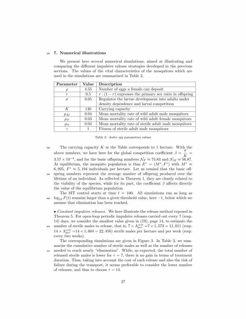
We present here several numerical simulations, aimed at illustrating andcomparing the different impulsive release strategies developed in the previoussections. The values of the vital characteristics of the mosquitoes which areused in the simulations are summarized in Table 2.
Parameter Value Descriptionρ 4.55 Number of eggs a female can depositr 0.5 r : (1− r) expresses the primary sex ratio in offspringσ 0.05 Regulates the larvae development into adults under
density dependence and larval competitionK 140 Carrying capacityµM 0.04 Mean mortality rate of wild adult male mosquitoesµF 0.03 Mean mortality rate of wild adult female mosquitoesµS 0.04 Mean mortality rate of sterile adult male mosquitoesγ 1 Fitness of sterile adult male mosquitoes
Table 2: Aedes spp parameters values
The carrying capacity K in the Table corresponds to 1 hectare. With the390
above numbers, we have here for the global competition coefficient β =σ
K=
3.57× 10⁻⁴, and for the basic offspring numbers NF ≈ 75.83 and NM ≈ 56.87.At equilibrium, the mosquito population is thus E∗ = (M∗, F ∗) with M∗ ≈6, 925, F ∗ ≈ 5, 194 individuals per hectare. Let us remind that the basic off-spring numbers represent the average number of offspring produced over the395
lifetime of an individual. As reflected in Theorem 1, they are closely related tothe viability of the species, while for its part, the coefficient β affects directlythe value of the equilibrium population.
The SIT control starts at time t = 100. All simulations run as long aslog10 F (t) remains larger than a given threshold value, here −1, below which we400
assume that elimination has been reached.
• Constant impulsive releases. We here illustrate the release method exposed inTheorem 5. For open-loop periodic impulsive releases carried out every 7 (resp.14) days, we consider the smallest value given in (19), page 14, to estimate thenumber of sterile males to release, that is, 7× Λcritper =7× 1, 573 = 11, 011 (resp.405
14× Λcritper =14× 1, 604 = 22, 456) sterile males per hectare and per week (resp.every two weeks).
The corresponding simulations are given in Figure 3. In Table 3, we sum-marize the cumulative number of sterile males as well as the number of releasesneeded to reach nearly “elimination”. While, as expected, the total number of410
released sterile males is lower for τ = 7, there is no gain in terms of treatmentduration. Thus, taking into account the cost of each release and also the risk offailure during the transport, it seems preferable to consider the lower numberof releases, and thus to choose τ = 14.
27

0 100 200 300 400 500 600 700
time (days)
-3
-2
-1
0
1
2
3
4
5
Log
10(N
um
ber
of In
div
iduals
)Male
Female
Sterile Male
0 100 200 300 400 500 600 700 800
time (days)
-3
-2
-1
0
1
2
3
4
5
Log
10(N
um
ber
of In
div
iduals
)
Male
Female
Sterile Male
(a) (b)
Figure 3: Open-loop periodic impulsive SIT control of system (15) with a period of: (a) 7days, (b) 14 days.
Period (days) Cumulative Number of Nb of Weeksreleased sterile males to reach elimination
τ = 7 924,627 84τ = 14 942, 869 84
Table 3: Cumulative number of released sterile males for each open-loop periodic SIT controltreatment.
The closed-loop approach can be used to reduce the cumulative number of415
released sterile insects and the number of effective releases. Further on, we willconsider several sub-cases.
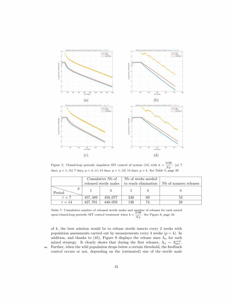
• Impulsive feedback control. We now show application of the algorithms givenin Theorems 6 and 7. Here and in the study of all feedback methods, we considermeasurements of the wild population every τ days or every pτ days for p = 4.Also, in order to display the tradeoff between treatment duration and controleffort, we investigate two values of k, namely
kNF = 0.2 and kNF = 0.99. (53)
With the smaller value k = 0.2/NF , the control effort is larger and one expectsfaster convergence toward E0 = (0, 0), at the price of larger releases of sterilemales, i.e. higher costs. On the contrary, for larger k = 0.99/NF , the control420
effort is smaller and convergence should be slower, with smaller total number ofreleased insects.
The size Λn of the n-th release is taken equal to the right-hand side offormula (39a) for p = 1 (of (45a) for p = 4): if, at the moment of the estimate,the size of the sterile male population is sufficiently large, Λn may be small or425
even null.Simulations presented in Figures 4 (page 30) and 5 (page 31) clearly show
that the choice of k and p, as well as the period τ of the releases play an
28

important role in the convergence of the wild population to E∗0 . Tables 4 and5 provide the total cumulative number of released sterile males, the number of430
weeks of SIT treatment needed to reach elimination, and the number of effective
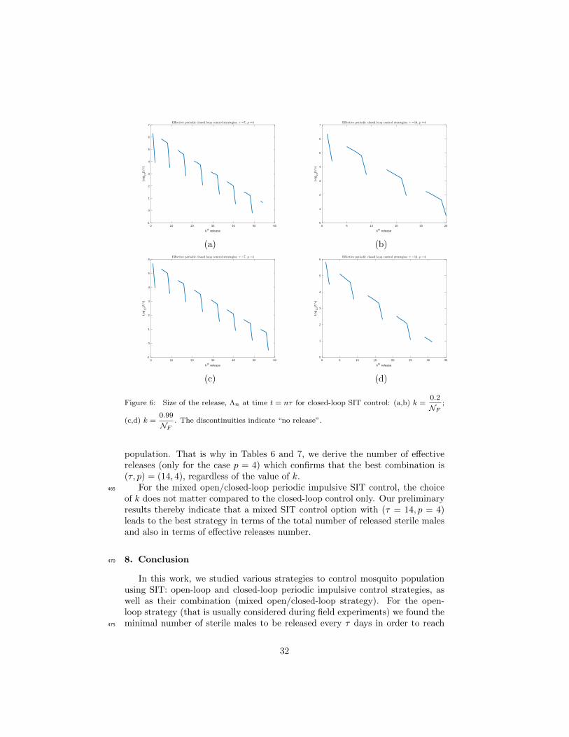
(that is nonzero) releases. For instance, when (τ, p) = (14, 4) and k =0.2
NFis
relatively small, elimination of wild mosquitoes can be achieved in 56 weeks,with only 17 effective releases, as shown in Fig. 6(b), page 32. However, thisoption requires to release significant number of sterile insects per hectare (close435
to 2.9× 10⁶ for the whole treatment).
For the larger k =0.99
NFand with (τ, p) = (7, 1) (see Figure 5(a)), the
convergence is slower: more than 240 weeks of SIT treatment are required toreach nearly elimination. For p = 4 (see Figure 5(b)), the wild population isclose to extinction after 58 weeks of SIT treatment. However, based on Table440
5, it seems that the choice (τ, p) = (14, 4) leads to the best result in terms oftiming (62 weeks) and also in terms of cumulative size encompassing 20 effectivereleases.
The parameter k is of main importance: when p = 4, while the number ofweeks to reach elimination is quite similar for both values of τ , the cumulative445
number of released sterile males is clearly smaller when k is closer to 1/NF .
Cumulative Nb of Nb of weeks toreleased sterile males reach elimination Nb of nonzero releases
Periodp
1 4 1 4 4
τ = 7 2, 251, 052 4, 363, 430 64 54 34τ = 14 2, 390, 676 2, 896, 835 64 56 17
Table 4: Cumulative number of released sterile males and number of releases for each closed-
loop periodic SIT control treatment when k =0.2
NF. See Figure 4, page 30.
Cumulative Nb of Nb of weeks neededreleased sterile males to reach elimination Nb of nonzero releases
Periodp
1 4 1 4 4
τ = 7 794, 807 1, 221, 593 240 58 37τ = 14 909, 344 1, 043, 107 130 62 20
Table 5: Cumulative number of released sterile males and number of releases for each closed-
loop periodic SIT control treatment when k =0.99
NF. See Figure 5, page 31
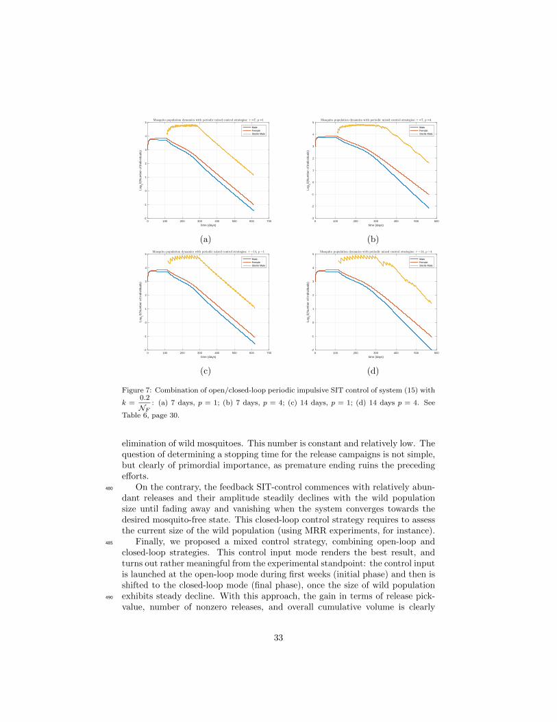
• Mixed control. We now consider mixed control strategies as exposed in Section6 (Theorem 8). In Figures 7 and 8 (pages 33 and 34, respectively) are shown thesimulations obtained with the same two underlying values of k given in (53).
29

0 100 200 300 400 500 600
time (days)
-2
-1
0
1
2
3
4
5
6
7
Log
10(N
umbe
r of
Indi
vidu
als)
MaleFemaleSterile Male
0 50 100 150 200 250 300 350 400 450 500
time (days)
-3
-2
-1
0
1
2
3
4
5
6
7
Log
10(N
umbe
r of
Indi
vidu
als)
MaleFemaleSterile Male
(a) (b)
0 100 200 300 400 500 600
time (days)
-2
-1
0
1
2
3
4
5
6
7
Log
10(N
umbe
r of
Indi
vidu
als)
MaleFemaleSterile Male
0 100 200 300 400 500 600
time (days)
-3
-2
-1
0
1
2
3
4
5
6
7
Log
10(N
umbe
r of
Indi
vidu
als)
MaleFemaleSterile Male
(c) (d)
Figure 4: Closed-loop periodic impulsive SIT control of system (15) with k =0.2
NF: (a) 7 days,
p = 1; (b) 7 days, p = 4; (c) 14 days, p = 1; (d) 14 days, p = 4. See Table 4, page 29
Cumulative Nb of Nb of weeks neededreleased sterile males to reach elimination Nb of nonzero releases
Periodp
1 4 1 4 4
τ = 7 450, 668 534, 849 72 65 53τ = 14 465, 187 499, 497 72 66 25
Table 6: Cumulative number of released sterile males and number of releases for each mixed
open/closed-loop periodic SIT control treatment when k =0.2
NF. See Figure 7, page 33.
Except for the case with (τ, p) = (7, 1) and k =0.99
NF(see Table 6, page 30),450
where the convergence to E∗0 is slow, it turns out that the mixed open/closed-loop control strategies derive the best results, not only in terms of releasesnumber but also in terms of overall cumulative number of sterile males to bereleased.
According to Tables 6 and 7 (pages 30 and 31, respectively), for both values455
30
0 200 400 600 800 1000 1200 1400 1600 1800
time (days)
-2
-1
0
1
2
3
4
5
6
Log
10(N
umbe
r of
Indi
vidu
als)
MaleFemaleSterile Male
0 100 200 300 400 500 600
time (days)
-2
-1
0
1
2
3
4
5
6
Log
10(N
umbe
r of
Indi
vidu
als)
MaleFemaleSterile Male
(a) (b)
0 200 400 600 800 1000 1200
time (days)
-2
-1
0
1
2
3
4
5
6
Log
10(N
umbe
r of
Indi
vidu
als)
MaleFemaleSterile Male
0 100 200 300 400 500 600
time (days)
-2
-1
0
1
2
3
4
5
6
Log
10(N
umbe
r of
Indi
vidu
als)
MaleFemaleSterile Male
(c) (d)
Figure 5: Closed-loop periodic impulsive SIT control of system (15) with k =0.99
NF: (a) 7
days, p = 1; (b) 7 days, p = 4; (c) 14 days, p = 1; (d) 14 days, p = 4. See Table 5, page 29
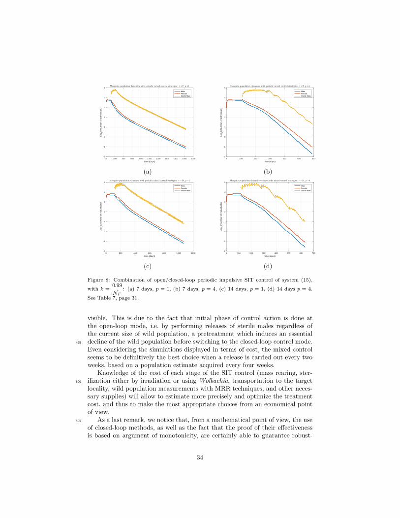
Cumulative Nb of Nb of weeks neededreleased sterile males to reach elimination Nb of nonzero releases
Periodp
1 4 1 4 4
τ = 7 457, 489 450, 077 246 69 53τ = 14 427, 701 449, 059 136 74 28
Table 7: Cumulative number of released sterile males and number of releases for each mixed
open/closed-loop periodic SIT control treatment when k =0.99
NF. See Figure 8, page 34.
of k, the best solution would be to release sterile insects every 2 weeks withpopulation assessments carried out by measurements every 4 weeks (p = 4). Inaddition, and thanks to (45), Figure 9 displays the release sizes Λn for eachmixed strategy. It clearly shows that during the first releases, Λn = Λcritper .Further, when the wild population drops below a certain threshold, the feedback460
control occurs or not, depending on the (estimated) size of the sterile male
31
0 10 20 30 40 50 60
kth release
-1
0
1
2
3
4
5
6
7
Log
10(
*)
0 5 10 15 20 25
kth release
0
1
2
3
4
5
6
7
Log
10(
*)
(a) (b)
0 10 20 30 40 50 60
kth release
-1
0
1
2
3
4
5
6
Log
10(
*)
0 5 10 15 20 25 30 35
kth release
0
1
2
3
4
5
6
Log
10(
*)
(c) (d)
Figure 6: Size of the release, Λn at time t = nτ for closed-loop SIT control: (a,b) k =0.2
NF;
(c,d) k =0.99
NF. The discontinuities indicate “no release”.
population. That is why in Tables 6 and 7, we derive the number of effectivereleases (only for the case p = 4) which confirms that the best combination is(τ, p) = (14, 4), regardless of the value of k.
For the mixed open/closed-loop periodic impulsive SIT control, the choice465
of k does not matter compared to the closed-loop control only. Our preliminaryresults thereby indicate that a mixed SIT control option with (τ = 14, p = 4)leads to the best strategy in terms of the total number of released sterile malesand also in terms of effective releases number.
8. Conclusion470
In this work, we studied various strategies to control mosquito populationusing SIT: open-loop and closed-loop periodic impulsive control strategies, aswell as their combination (mixed open/closed-loop strategy). For the open-loop strategy (that is usually considered during field experiments) we found theminimal number of sterile males to be released every τ days in order to reach475
32
0 100 200 300 400 500 600 700
time (days)
-2
-1
0
1
2
3
4
5
Log
10(N
umbe
r of
Indi
vidu
als)
MaleFemaleSterile Male
0 100 200 300 400 500 600
time (days)
-3
-2
-1
0
1
2
3
4
5
Log
10(N
umbe
r of
Indi
vidu
als)
MaleFemaleSterile Male
(a) (b)
0 100 200 300 400 500 600 700
time (days)
-2
-1
0
1
2
3
4
5
Log
10(N
umbe
r of
Indi
vidu
als)
MaleFemaleSterile Male
0 100 200 300 400 500 600
time (days)
-2
-1
0
1
2
3
4
5
Log
10(N
umbe
r of
Indi
vidu
als)
MaleFemaleSterile Male
(c) (d)
Figure 7: Combination of open/closed-loop periodic impulsive SIT control of system (15) with
k =0.2
NF: (a) 7 days, p = 1; (b) 7 days, p = 4; (c) 14 days, p = 1; (d) 14 days p = 4. See
Table 6, page 30.
elimination of wild mosquitoes. This number is constant and relatively low. Thequestion of determining a stopping time for the release campaigns is not simple,but clearly of primordial importance, as premature ending ruins the precedingefforts.
On the contrary, the feedback SIT-control commences with relatively abun-480
dant releases and their amplitude steadily declines with the wild populationsize until fading away and vanishing when the system converges towards thedesired mosquito-free state. This closed-loop control strategy requires to assessthe current size of the wild population (using MRR experiments, for instance).
Finally, we proposed a mixed control strategy, combining open-loop and485
closed-loop strategies. This control input mode renders the best result, andturns out rather meaningful from the experimental standpoint: the control inputis launched at the open-loop mode during first weeks (initial phase) and then isshifted to the closed-loop mode (final phase), once the size of wild populationexhibits steady decline. With this approach, the gain in terms of release pick-490
value, number of nonzero releases, and overall cumulative volume is clearly
33
0 200 400 600 800 1000 1200 1400 1600 1800 2000
time (days)
-2
-1
0
1
2
3
4
5
Log
10(N
umbe
r of
Indi
vidu
als)
MaleFemaleSterile Male
0 100 200 300 400 500 600
time (days)
-2
-1
0
1
2
3
4
5
Log
10(N
umbe
r of
Indi
vidu
als)
MaleFemaleSterile Male
(a) (b)
0 200 400 600 800 1000 1200
time (days)
-2
-1
0
1
2
3
4
5
Log
10(N
umbe
r of
Indi
vidu
als)
MaleFemaleSterile Male
0 100 200 300 400 500 600 700
time (days)
-2
-1
0
1
2
3
4
5
Log
10(N
umbe
r of
Indi
vidu
als)
MaleFemaleSterile Male
(c) (d)
Figure 8: Combination of open/closed-loop periodic impulsive SIT control of system (15),
with k =0.99
NF: (a) 7 days, p = 1, (b) 7 days, p = 4, (c) 14 days, p = 1, (d) 14 days p = 4.
See Table 7, page 31.
visible. This is due to the fact that initial phase of control action is done atthe open-loop mode, i.e. by performing releases of sterile males regardless ofthe current size of wild population, a pretreatment which induces an essentialdecline of the wild population before switching to the closed-loop control mode.495
Even considering the simulations displayed in terms of cost, the mixed controlseems to be definitively the best choice when a release is carried out every twoweeks, based on a population estimate acquired every four weeks.
Knowledge of the cost of each stage of the SIT control (mass rearing, ster-ilization either by irradiation or using Wolbachia, transportation to the target500
locality, wild population measurements with MRR techniques, and other neces-sary supplies) will allow to estimate more precisely and optimize the treatmentcost, and thus to make the most appropriate choices from an economical pointof view.
As a last remark, we notice that, from a mathematical point of view, the use505
of closed-loop methods, as well as the fact that the proof of their effectivenessis based on argument of monotonicity, are certainly able to guarantee robust-
34

0 10 20 30 40 50 60 70
kth release
-0.5
0
0.5
1
1.5
2
2.5
3
3.5
4
4.5
Log
10(
*)
0 5 10 15 20 25 30 35
kth release
0.5
1
1.5
2
2.5
3
3.5
4
4.5
5
Log
10(
*)
(a) (b)
0 10 20 30 40 50 60 70
kth release
-1
0
1
2
3
4
5
Log
10(
*)
0 5 10 15 20 25 30 35 40
kth release
0.5
1
1.5
2
2.5
3
3.5
4
4.5
5
Log
10(
*)
(c) (d)
Figure 9: Size of the release, Λn, at time t = nτ for mixed open/closed-loop SIT control:
(a,b) k =0.2
NF; (c,d) k =
0.99
NF. The discontinuities indicate “no release”.
ness of the proposed closed-loop algorithms with respect to several uncertaintiespresent in the problem under study. In particular, it is believed that the frame-work developed here could most certainly be extended to consider the effects510
of modeling and measurement errors, as well as imprecision and delay in thecontrol-loop.
Acknowledgments
Support from the Colciencias – ECOS-Nord Program (Colombia: ProjectCI-71089; France: Project C17M01) is kindly acknowledged. DC and OV515
were supported by the inter-institutional cooperation program MathAmsud (18-MATH-05). This study was part of the Phase 2A ‘SIT feasibility project againstAedes albopictus in Reunion Island’, jointly funded by the French Ministry ofHealth (Convention 3800/TIS) and the European Regional Development Fund
35

(ERDF) (Convention No. 2012-32122 and Convention No. GURDTI 2017-0583-520
0001899). YD was (partially) supported by the DST/NRF SARChI Chair inMathematical Models and Methods in Biosciences and Bioengineering at theUniversity of Pretoria (grant 82770). YD also acknowledges the support ofthe Visiting Professor Granting Scheme from the Office of the Deputy Vice-Chancellor for Research Office of the University of Pretoria.525
[1] V. A. Dyck, J. Hendrichs, A. S. Robinson, The Sterile Insect Tech-nique, Principles and Practice in Area-Wide Integrated Pest Management,Springer, Dordrecht, 2006.
[2] M. Hertig, S. B. Wolbach, Studies on rickettsia-like micro-organisms ininsects, The Journal of medical research 44 (3) (1924) 329.530
[3] K. Bourtzis, Wolbachia-based technologies for insect pest population con-trol, in: Advances in Experimental Medicine and Biology, Vol. 627,Springer, New York, NY, 2008.
[4] S. P. Sinkins, Wolbachia and cytoplasmic incompatibility in mosquitoes,Insect Biochemistry and Molecular Biology 34 (7) (2004) 723 – 729, molec-535
ular and population biology of mosquitoes.
[5] J. L. Rasgon, T. W. Scott, Wolbachia and cytoplasmic incompatibilityin the California Culex pipiens mosquito species complex: parameter es-timates and infection dynamics in natural populations, Genetics 165 (4)(2003) 2029–2038.540
[6] J. G. Schraiber, A. N. Kaczmarczyk, R. Kwok, M. Park, R. Silverstein,F. U. Rutaganira, T. Aggarwal, M. A. Schwemmer, C. L. Hom, R. K. Gros-berg, S. J. Schreiber, Constraints on the use of lifespan-shortening Wol-bachia to control dengue fever, Journal of Theoretical Biology 297 (2012)26 – 32.545
[7] L. A. Moreira, I. Iturbe-Ormaetxe, J. A. Jeffery, G. Lu, A. T. Pyke, L. M.Hedges, B. C. Rocha, S. Hall-Mendelin, A. Day, M. Riegler, L. E. Hugo,K. N. Johnson, B. H. Kay, E. A. McGraw, A. F. van den Hurk, P. A. Ryan,S. L. O’Neill, A Wolbachia symbiont in Aedes aegypti limits infection withdengue, chikungunya, and plasmodium, Cell 139 (7) (2009) 1268 – 1278.550
[8] C. Dufourd, Y. Dumont, Modeling and simulations of mosquito dispersal.the case of Aedes albopictus, Biomath 1209262 (2012) 1–7.
[9] C. Dufourd, Y. Dumont, Impact of environmental factors on mosquito dis-persal in the prospect of sterile insect technique control, Comput. Math.Appl. 66 (9) (2013) 1695–1715.555
[10] Y. Dumont, J. M. Tchuenche, Mathematical studies on the sterile insecttechnique for the Chikungunya disease and Aedes albopictus, Journal ofMathematical Biology 65 (5) (2012) 809–855.
36

[11] M. Huang, X. Song, J. Li, Modelling and analysis of impulsive releases ofsterile mosquitoes, Journal of Biological Dynamics 11 (1) (2017) 147–171.560
[12] J. Li, Z. Yuan, Modelling releases of sterile mosquitoes with different strate-gies, Journal of Biological Dynamics 9 (1) (2015) 1–14.
[13] M. Strugarek, H. Bossin, Y. Dumont, On the use of the sterile insect releasetechnique to reduce or eliminate mosquito populations, Applied Mathe-matical Modellingdoi:https://doi.org/10.1016/j.apm.2018.11.026.565
URL http://www.sciencedirect.com/science/article/pii/
S0307904X18305638
[14] D. E. Campo-Duarte, D. Cardona-Salgado, O. Vasilieva, EstablishingwMelPop Wolbachia infection among wild Aedes aegypti females by op-timal control approach, Applied Mathematics and Information Sciences570
11 (4) (2017) 1011–1027. doi:10.18576/amis/110408.
[15] D. E. Campo-Duarte, O. Vasilieva, D. Cardona-Salgado, M. Svinin, Opti-mal control approach for establishing wMelPop Wolbachia infection amongwild Aedes aegypti populations, Journal of mathematical biology 76 (7)(2018) 1907–1950.575
[16] J. Z. Farkas, S. A. Gourley, R. Liu, A.-A. Yakubu, Modelling Wolbachiainfection in a sex-structured mosquito population carrying West Nile virus,Journal of Mathematical Biology 75 (3) (2017) 621–647.
[17] J. Z. Farkas, P. Hinow, Structured and unstructured continuous modelsfor Wolbachia infections, Bulletin of Mathematical Biology 72 (8) (2010)580
2067–2088.
[18] A. Fenton, K. N. Johnson, J. C. Brownlie, G. D. D. Hurst, Solving theWolbachia paradox: modeling the tripartite interaction between host, Wol-bachia, and a natural enemy, The American Naturalist 178 (2011) 333–342.
[19] H. Hughes, N. F. Britton, Modeling the Use of Wolbachia to Control585
Dengue Fever Transmission, Bull. Math. Biol. 75 (2013) 796–818.
[20] G. Nadin, M. Strugarek, N. Vauchelet, Hindrances to bistable front propa-gation: application to Wolbachia invasion, Journal of Mathematical Biology76 (6) (2018) 1489–1533. doi:10.1007/s00285-017-1181-y.URL https://doi.org/10.1007/s00285-017-1181-y590
[21] M. Strugarek, N. Vauchelet, J. Zubelli, Quantifying the survival uncer-tainty of Wolbachia-infected mosquitoes in a spatial model, MathematicalBiosciences and Engineering 15(4) (2018) 961–991.
[22] H. L. Smith, Monotone Dynamical Systems: An Introduction to the The-ory of Competitive and Cooperative Systems, Providence, R.I.: American595
Mathematical Society, 1995.
37

[23] R. Anguelov, Y. Dumont, J. Lubuma, Mathematical modeling of sterileinsect technology for control of Anopheles mosquito, Comput. Math. Appl.64 (3) (2012) 374–389.
[24] J. Koiller, M. Da Silva, M. Souza, C. Codeco, A. Iggidr, G. Sallet, Aedes,600
Wolbachia and Dengue, Research Report RR-8462, Inria Nancy - GrandEst (Villers-les-Nancy, France) (Jan. 2014).URL https://hal.inria.fr/hal-00939411
[25] P.-A. Bliman, M. S. Aronna, F. C. Coelho, M. A. H. B. da Silva, Ensur-ing successful introduction of Wolbachia in natural populations of Aedes605
aegypti by means of feedback control, Journal of Mathematical Biology76 (5) (2018) 1269–1300.
[26] P.-A. Bliman, Feedback control principles for biological control of denguevectors, arXiv preprint arXiv:1903.00730.
[27] L. Gouagna, J. Dehecq, D. Fontenille, Y. Dumont, S. Boyer, Seasonal vari-610
ation in size estimates of Aedes albopictus population based on standardmark-release-recapture experiments in an urban area on Reunion Island,Acta Tropica 143 (2015) 89–96.
[28] K. Cooke, P. van den Driessche, X. Zou, Interaction of maturation delayand nonlinear birth in population and epidemic models, Journal of Math-615
ematical Biology 39 (4) (1999) 332–352. doi:10.1007/s002850050194.URL https://doi.org/10.1007/s002850050194
[29] L. Perko, Differential Equations and Dynamical Systems, Springer-Verlag,2006.
38

Appendix: Proof of Lemma 1, page 11620
First, it is easy to check that function f , defined in (14), page 11, is firstdecreasing and then increasing, and, thus, may solely have no root, one root ortwo zeros.
On the other hand, the number of roots of f(x) = 0 is clearly non-increasingwith respect to a > 0: it has two roots for ‘small values’ of a, no root for ‘largevalues’ of a, and exactly one root for a certain critical value acrit separatingthe two previous regions. This critical value is characterized by the fact that itpossesses a double root xcrit > 0, such that f(xcrit) = f ′(xcrit) = 0, that is:
1 +acrit
xcrit= NF e−cx
crit
,acrit
(xcrit)2= NF ce−cx
crit
. (A-1)
Eliminating the exponential term in the previous formulas yields the second-
order polynomial equation in1
xcrit(1
xcrit
)2
− c
xcrit− c
acrit= 0.
Its unique positive root is
1
xcrit=
c+
√c2 + 4
c
acrit
2=c
2
(1 +
√1 +
4
acritc
),
that is:
xcrit :=2
c
1
1 +
√1 +
4
acritc
.
Introducing this expression back in (A-1), leads to
1 +acritc
2
(1 +
√1 +
4
acritc
)= NF exp
− 2
1 +√
1 + 4acritc
.Thus φcrit :=
acritc
2is solution of (11), page 10, such that, at the critical point,
the parameters acrit,NF , c are interrelated.625
For positive values of a smaller than acrit, the equation f(x) = 0 has tworoots, and no root whenever a > acrit. This achieves the proof of Lemma 1.
39