Implementation of the Nitrate Pollution Prevention Regulations 2015 in England Method for designating Nitrate Vulnerable Zones for groundwaters December 2016

© Crown copyright 2016

You may re-use this information (excluding logos) free of charge in any format or medium, under the terms of the Open Government Licence v.3. To view this licence visit www.nationalarchives.gov.uk/doc/open-government-licence/version/3/ or email PSI@nationalarchives.gsi.gov.uk

This publication is available at www.gov.uk/government/publications

Any enquiries regarding this publication should be sent to us at

enquiries@environment-agency.gov.uk

www.gov.uk/defra

Contents

1. Introduction and overview ............................................................................................. 1

1.2 Background ............................................................................................................ 1

1.3 Criteria for identifying polluted waters ..................................................................... 1

1.4 Evolution of assessment methodology ................................................................... 2

1.5 Structure of the report ............................................................................................. 2

2. Overview of the Method ................................................................................................ 2

2.1 Introduction ............................................................................................................. 2

2.2 Base mapping and other basic environmental datasets ......................................... 3

2.3 Nitrate loads applied to ground ............................................................................... 3

2.4 Monitored nitrate concentrations ............................................................................. 4

2.5 Interpolated nitrate concentrations .......................................................................... 6

2.6 Risk assessment – national scale ........................................................................... 7

2.7 Local Area workshops ............................................................................................ 8

2.8 Final mapping ......................................................................................................... 9

2.9 Method summary .................................................................................................... 9

3. Combining the evidence ............................................................................................. 13

3.1 Introduction ........................................................................................................... 13

3.2 Risk model components, scores and weightings .................................................. 14

3.3 Combined risk assessment ................................................................................... 19

4. Identifying land draining to polluted waters ................................................................. 20

References ........................................................................................................................ 21

Appendix A ........................................................................................................................ 22

A1 What form of nitrogenous compounds do we refer to in this assessment? ........... 22

A2 Why do we use the 95th percentile to characterise water quality for NVZs? ......... 22

A3 Explanation of the Weibull method ....................................................................... 23

Appendix B Nitrate attenuation and dilution ....................................................................... 24

B1 What is denitrification? .......................................................................................... 25

B2 What is groundwater mixing?................................................................................ 25

Appendix C Hard boundary conversion rule ...................................................................... 26

1

1. Introduction and overview The Nitrates Directive (91/676/EEC) require nitrate vulnerable zones to be reviewed every four years. This report sets out the method used to derive and delineate Nitrate Vulnerable Zones (NVZs) for groundwaters for the 2017 review in England. This is referred to as the 2017 review because the resulting designations are due to come into force in January 2017.

The method uses a range of national datasets (for example, geological and hydrological maps) combined with analysis of farm-derived nitrate loadings (from farm census returns) and monitored concentrations in groundwater. In line with standard practice, the method depends on a conceptual understanding of the groundwater in a particular location, as well the local knowledge of our Area operational staff.

Short summary diagrams are included to give a quick overview of the process, but the report is intended for a broadly technical readership.

1.2 Background The Nitrates Directive (91/676/EEC) is intended to protect waters against nitrate pollution from agricultural sources. Member States are required to identify waters which are, or could become, polluted by nitrates and to designate all land draining to these waters and contributing to the pollution as Nitrate Vulnerable Zones (NVZs). Farmers in designated areas must then follow an Action Programme to reduce pollution from agricultural sources of nitrate. The criteria for identifying waters as polluted are established in the Directive. The Nitrate Pollution Prevention Regulations 2015, which transpose the Directive into domestic law, require the Agency to make recommendations to the Secretary of State as to areas of land which should be, or should continue to be, designated as NVZs.

The assessment method described here builds on the experience of earlier NVZ designation rounds (Defra, 2008 and Environment Agency, 2008). It adopts a weight of evidence approach that aims to protect groundwater where needed whilst not imposing regulation where not needed.

1.3 Criteria for identifying polluted waters The Nitrate Pollution Prevention Regulations 2015 require us to identify groundwater which contains more than 50 mg/l nitrate (as NO3), or could do so if preventative measures are not adopted. In making the assessment we take into account:

• the physical and environmental characteristics of the water and land;

2

• the behaviour of nitrogen compounds in the environment ;

• our understanding of the impact of preventative action.

• changes and factors unforeseen at the previous review .

The periodic nature of reviewing NVZs means that each review presents an assessment of nitrate pollution up to the time of the review.

1.4 Evolution of assessment methodology NVZ reviews were carried out in 1993, 1996, 2002, 2008 and 2013. For 2008 a new risk model approach was adopted and this method, with some modifications was also used for 2013. We have adopted a similar approach for NVZ 2017 designations but using updated datasets where these are available and modifying the method to take account of some of the lessons learned in the previous rounds and relevant developments in scientific understanding of nitrate in the environment.

1.5 Structure of the report The remainder of this report is divided into an overview of the method and then the detailed description of the risk parameters used. Further technical material is presented in the Appendices. Much of the statistical analysis used in the assessment was carried out under contract by WRc plc and a detailed report of this work is available (WRc 2015).

2. Overview of the Method

2.1 Introduction The method for determining the groundwater NVZ designations relies on combining a number of datasets and uses our understanding of the behaviour of groundwater and nitrate both in general and in particular locations.

The method generates geological, geographical or hydrological boundaries, which we call ‘soft boundaries’. In NVZs, since the measures farmers take are at field scale, these boundaries are then aligned to the nearest field boundaries to form the final ‘hard boundary’.

3

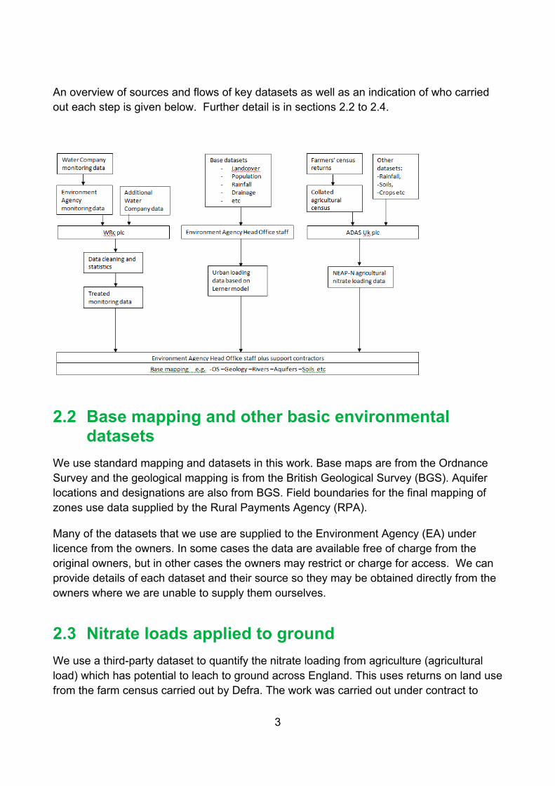
An overview of sources and flows of key datasets as well as an indication of who carried out each step is given below. Further detail is in sections 2.2 to 2.4.

2.2 Base mapping and other basic environmental datasets

We use standard mapping and datasets in this work. Base maps are from the Ordnance Survey and the geological mapping is from the British Geological Survey (BGS). Aquifer locations and designations are also from BGS. Field boundaries for the final mapping of zones use data supplied by the Rural Payments Agency (RPA).

Many of the datasets that we use are supplied to the Environment Agency (EA) under licence from the owners. In some cases the data are available free of charge from the original owners, but in other cases the owners may restrict or charge for access. We can provide details of each dataset and their source so they may be obtained directly from the owners where we are unable to supply them ourselves.

2.3 Nitrate loads applied to ground We use a third-party dataset to quantify the nitrate loading from agriculture (agricultural load) which has potential to leach to ground across England. This uses returns on land use from the farm census carried out by Defra. The work was carried out under contract to

4

Defra by ADAS UK plc and the results supplied to the Environment Agency in digital form. A fuller description of the work is given in the report from ADAS (Lee et al, 2015) but a brief summary is provided here.

Nitrate leaching from agricultural land was calculated using NEAP-N (Lord and Anthony 2000) based on agricultural census data from the ADAS National Land Use database, soils data from the NSRI LAND-IS database and climate data from the UK-CIP. Nitrate losses were calculated at a spatial resolution of 1 km2 under average climate conditions. NEAP-N calculates agricultural loads using a single maximum potential nitrogen loss coefficient for individual crop and livestock types, modified by soil type and hydrologically effective rainfall (HER). Total values for agricultural nitrate were calculated and losses were standardised by dividing by rainfall for each 1 km2 cell. To deal with uncertainty in the data coverage, each cell was averaged with its direct neighbouring cells.

The data from ADAS is in the form of a 1 km grid across England with nitrate concentrations from the different sources identified. The 1 km scale is important and determines the scale for considering the monitored nitrate concentrations in groundwater below.

Nitrate leaching from non-agricultural “urban” land areas (non-agricultural or urban loads) was calculated according to the component model of Lerner (2000). Nitrate losses to groundwater are expressed as export coefficients per hectare of each urban land cover type. The model identifies 14 components of runoff, although not all were included in the data for this method. We updated the urban loading using the same procedure as in previous reviews but replaced the Land Cover map (CEH) from 2000 with the latest dataset 2007 and the CORINE data (European Environment Agency, 2000 updated to 2006). This is converted to concentrations using the Hydrologically Effective Rainfall (HER) values from the Continuous Estimation of River Flows (CERF) model developed by the Centre for Ecology and Hydrology. Population data from 2001 census was updated with 2011 census data.

2.4 Monitored nitrate concentrations The EA maintains a strategic groundwater quality monitoring network that is designed to help deliver the requirements of the WFD. In addition, we collect groundwater samples associated with a range of activities and for a range of other purposes.

Water quality monitoring data was supplied from the EA’s Water Information Management System (WIMS) database with additional data supplied by Water Companies in England and Wales. The data was cleaned and then analysed by WRc plc under contract. The output was a calculation of the current and future 95th percentile nitrate concentration at each individual monitoring point. For an explanation of why we use the 95th percentile refer to Appendix A.

5

All groundwater monitoring points with sufficient data were analysed using a suite of tools similar to those used in previous reviews. However, these have been recoded into “R” where this would improve efficiency. Full details of the analyses are given in the accompanying WRc report (WRc 2015) but some of the changes made from the 2013 review are highlighted here.

The tool “AntC2” was discontinued. This is very rarely used and WRc advised based on the experience in the 2013 designations that predictions from AntC2 typically provide no improved predictions compared to the simpler direct estimation of the mean. Only 15 sites were analysed by AntC2 for the 2013 review, and only 28 GW sites meet the criteria for AntC2 in this 2017 review. These sites were still analysed but using one of the other approaches.

The statistical methods used in the 2013 review assumed that the measured groundwater nitrate concentrations from an individual sampling point are from a single population with a normal distribution. That is, the samples taken at different times from the same borehole (or spring) are related. Whilst this is a reasonable assumption in most cases, there are a few sites where this appears not to be true. It is possible for different groundwater pathways to become activated (or quiescent) under different flow conditions, for example high water table versus low water table. As a result, groundwater from different locations, ages and chemistry may enter a single borehole at different times. We have introduced a statistical test to identify such sites. These sites were flagged for discussion at the local Area workshops.

The groundwater method compares the threshold of 50 mg/l (nitrate as NO3) with the lower 90% confidence limit (LCL) around the 95th percentile of the monitored nitrate sample distribution calculated using the Weibull method (see Appendix A for a description of this method). However, many groundwater monitoring points lack sufficient data to estimate the 95%ile concentration using this method. The solution, first used in the review for NVZ 2008, calculated the mean concentration for monitoring points lacking sufficient data and estimated the LCL based on a relationship calculated from all the sample points where there was sufficient data.

For the NVZ 2008 review the value of 42 or 43mg/l was determined and then adopted as 45 mg/l the “45 mg rule”. For the NVZ 2013 review an updated analysis again showed that the ratio between the mean and the LCL is always 1.16 and so when the LCL exactly equals the 50 mg/l threshold, the mean concentration is expected to be 43 mg/l. We adopted the threshold calculated from the analysis for NVZ 2013, that is, 43mg/l. Therefore in estimating the LCL for the 2017 designations we adopt the convention that: LCL = Mean x 1.16. Following this change WRc have updated this analysis with the new data (WRc 2016).

Note that, in common with our own and most external analytical laboratories, we have adopted the convention of reporting nitrate concentrations in terms of the mass of nitrogen present in nitrate (“nitrate as N”). Hence the drinking water standard of 50mg/l “nitrate as

6

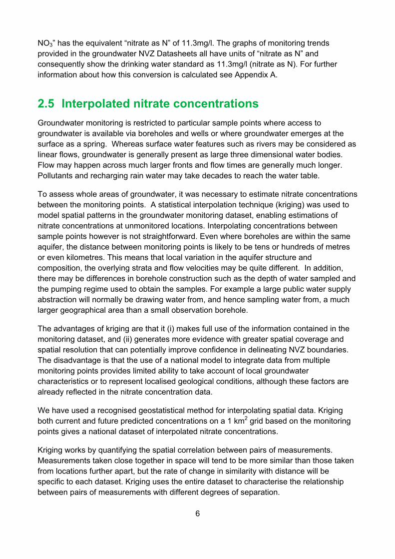
NO3” has the equivalent “nitrate as N” of 11.3mg/l. The graphs of monitoring trends provided in the groundwater NVZ Datasheets all have units of “nitrate as N” and consequently show the drinking water standard as 11.3mg/l (nitrate as N). For further information about how this conversion is calculated see Appendix A.

2.5 Interpolated nitrate concentrations Groundwater monitoring is restricted to particular sample points where access to groundwater is available via boreholes and wells or where groundwater emerges at the surface as a spring. Whereas surface water features such as rivers may be considered as linear flows, groundwater is generally present as large three dimensional water bodies. Flow may happen across much larger fronts and flow times are generally much longer. Pollutants and recharging rain water may take decades to reach the water table.

To assess whole areas of groundwater, it was necessary to estimate nitrate concentrations between the monitoring points. A statistical interpolation technique (kriging) was used to model spatial patterns in the groundwater monitoring dataset, enabling estimations of nitrate concentrations at unmonitored locations. Interpolating concentrations between sample points however is not straightforward. Even where boreholes are within the same aquifer, the distance between monitoring points is likely to be tens or hundreds of metres or even kilometres. This means that local variation in the aquifer structure and composition, the overlying strata and flow velocities may be quite different. In addition, there may be differences in borehole construction such as the depth of water sampled and the pumping regime used to obtain the samples. For example a large public water supply abstraction will normally be drawing water from, and hence sampling water from, a much larger geographical area than a small observation borehole.

The advantages of kriging are that it (i) makes full use of the information contained in the monitoring dataset, and (ii) generates more evidence with greater spatial coverage and spatial resolution that can potentially improve confidence in delineating NVZ boundaries. The disadvantage is that the use of a national model to integrate data from multiple monitoring points provides limited ability to take account of local groundwater characteristics or to represent localised geological conditions, although these factors are already reflected in the nitrate concentration data.

We have used a recognised geostatistical method for interpolating spatial data. Kriging both current and future predicted concentrations on a 1 km2 grid based on the monitoring points gives a national dataset of interpolated nitrate concentrations.

Kriging works by quantifying the spatial correlation between pairs of measurements. Measurements taken close together in space will tend to be more similar than those taken from locations further apart, but the rate of change in similarity with distance will be specific to each dataset. Kriging uses the entire dataset to characterise the relationship between pairs of measurements with different degrees of separation.

7

This modelled relationship (variogram) is then applied to estimate the measured variable at unmonitored locations from the values observed at surrounding locations. This is achieved by taking a weighted average of the measurements surrounding the unmonitored location. Decreasing weight is given to measurements further away from the unmonitored location, as determined by the spatial correlation relationship. This interpolation process is repeated for every cell of a grid to build up a complete two-dimensional map. It is possible to create and fit a number of relationships to the available data. We have chosen an approach that aims to reflect as closely as possible the presence of high concentration results in grid squares where monitored results are directly available. In addition, for grid squares containing a sample location exhibiting higher nitrate concentrations than the kriging interpolation, the concentration in that location has been adjusted to reflect the current or future concentration corresponding to that sample. The observed risk score is then calculated using the adjusted value.

Again the statistical calculations and kriging were carried out by WRc and details are in their report (WRc, 2015).

2.6 Risk assessment – national scale A numerical risk model was used to integrate the N loading and monitoring datasets and then incorporate any additional factors such as evidence of denitrification or unrepresentative monitoring. Weighted scores were applied to each 1 km square across England based on the values from the sections above. One of three levels of risk was assigned to each:

• High risk – both the N loading data and the monitored concentrations agree that nitrate concentrations exceed or were likely to exceed 11.3mg/l, and that agriculture was a significant source of the pollution identified.

• Medium risk– either the N loading data or the monitored concentrations show that nitrate concentrations exceed, or were likely to exceed, 11.3mg/l.

• Low risk– both the N loading data and the monitored concentrations agree that nitrate concentrations were not likely to exceed 11.3mg/l.

The scores were compiled as data for use in a geographical information system (GIS). We provided them to our local Area staff as GIS files or paper maps for discussion in local workshops. At the workshops scores could be modified to take account of additional local knowledge.

8

2.7 Local Area workshops A series of workshops with local EA staff provide more detailed local knowledge input to the review. Prior to the workshops our local staff received evidence from the national work detailed above. In general, discussions on individual zones were resolved at these face to face meetings. In some cases where further information or analysis was required, discussions continued via email or video conferences.

Various national datasets were used to inform this “ground-truthing” process, including: information on the sampling site (e.g. borehole construction details), knowledge of any local land use changes or concerns, local studies (e.g. porous pot sampling of recharge), solid geology, superficial geology (thickness, permeability), solution features, depth of unsaturated zone, groundwater head, surface water nitrate concentrations.

Modifications to the level of risk were made on the basis of local knowledge of the land and/or hydrogeology, for example through:

• Identification of point source pollution – if samples from a monitoring point were suspected of being unduly influenced by some non-agricultural, point source pollution then the level of risk could be downgraded.

• Understanding of the hydrogeology –the level of risk could be either downgraded or upgraded depending on the hydrogeological setting. For example:

o if a monitoring point takes samples from a deep confined aquifer it would not be representative of shallow unconfined groundwater quality above it, in this case the level of risk could be downgraded; or,

o if the monitoring data is for groundwater in a deep unconfined aquifer, with long lag times between pollution leaving the ground surface and being monitored in the groundwater, in this case the level of risk in the recharge area could be upgraded.

• If surface water monitoring is available in areas with infrequent groundwater monitoring then this data could be used to upgrade the level of risk where the data is representative of groundwater quality.

• If the processes of de-nitrification or mixing act to decrease nitrate concentrations before it reaches the groundwater then the level of risk could be downgraded.

Our Area groundwater specialists also identified appropriate zone boundaries based on the criteria set out below. Note that land that is directly above polluted groundwater does not necessarily drain into it. Similarly, groundwater may receive recharge water from land not directly above it. There are a number of factors affecting the path of water from the surface downwards into a groundwater body including, for example, the presence of

9

impermeable layers. Similarly, land that is not directly above a polluted groundwater may drain into it due to lateral flow within the soil or subsoil. Many of these factors are best understood by our local EA Area staff so determining what feature to use as a boundary was discussed with local EA staff. The boundaries so chosen became the “soft” boundaries for the proposed zones.

2.8 Final mapping The soft boundaries, in general, reflect geological or hydrological divides but these may not always be apparent at the land surface and hence could cause some difficulty in explaining and regulating on a farm by farm basis. Therefore, as a final step we map the soft zone boundaries to existing field boundaries based on map data provided by the Rural Payments Agency. The method used was developed for the 2013 designation round and is described in more detail in Appendix C.

2.9 Method summary The following 3 pages give a summary of the various stages of the method outlined above with comments.

The subsequent sections each give more detail about particular aspects of the method and the scoring system.

10

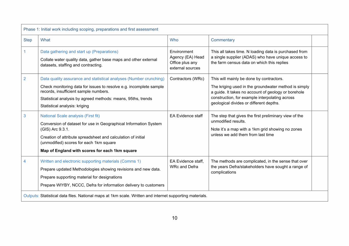
Phase 1: Initial work including scoping, preparations and first assessment

Step What Who Commentary

1 Data gathering and start up (Preparations)

Collate water quality data, gather base maps and other external datasets, staffing and contracting.

Environment Agency (EA) Head Office plus any external sources

This all takes time. N loading data is purchased from a single supplier (ADAS) who have unique access to the farm census data on which this replies

2 Data quality assurance and statistical analyses (Number crunching)

Check monitoring data for issues to resolve e.g. incomplete sample records, insufficient sample numbers.

Statistical analysis by agreed methods: means, 95ths, trends

Statistical analysis: kriging

Contractors (WRc) This will mainly be done by contractors.

The kriging used in the groundwater method is simply a guide. It takes no account of geology or borehole construction, for example interpolating across geological divides or different depths.

3 National Scale analysis (First fit)

Conversion of dataset for use in Geographical Information System (GIS) Arc 9.3.1.

Creation of attribute spreadsheet and calculation of initial (unmodified) scores for each 1km square

Map of England with scores for each 1km square

EA Evidence staff The step that gives the first preliminary view of the unmodified results.

Note it’s a map with a 1km grid showing no zones unless we add them from last time

4 Written and electronic supporting materials (Comms 1)

Prepare updated Methodologies showing revisions and new data.

Prepare supporting material for designations

Prepare WIYBY, NCCC, Defra for information delivery to customers

EA Evidence staff, WRc and Defra

The methods are complicated, in the sense that over the years Defra/stakeholders have sought a range of complications

Outputs: Statistical data files. National maps at 1km scale. Written and internet supporting materials.

11

Phase 2: Local workshops

Step What Who Commentary

6 Local workshops ( Face to face)

National team travel to each Area in turn to discuss and ‘groundtruth’ the first fit results from Phase 1.

Identify and confirm locations where zones are needed (or not) based on reaching a consensus understanding from groundwater there.

As we do not automatically use WFD boundaries for groundwater an important part of the workshop is to discuss the appropriate boundary locations based on the expert knowledge of the Area hydrogeologists. Likely boundaries are discussed in the Methodology.

Draft ’soft’ zone boundaries based on geology, hydrology etc

EA Area staff plus EA Evidence staff plus any external observers

This is intended as a very interactive and open discussion, We use multiple Agency and other datasets to help us understand the groundwater setting and results. For example, our information systems for boreholes, wells and springs contains details of borehole construction. We can look this up and consider issues such as depth to water, screening, liner etc to contrast with the kriging results. The process of designation is really about an expert judgement with some of the data formalised by the method.

7 Follow up (Clarification and snagging)

Resolve any outstanding issues that were raised at the workshops.

Collate a national set of soft zone boundaries

EA Evidence staff plus Contractors

We are unlikely to resolve all the issues in the workshop itself. This follow up work is to continue until each issue is resolved. It may mean additional visits to Area staff or may be resolved by email etc.

Outputs: Soft boundary map. Any notes from workshops

12

Phase 3: Mapping

Step What Who Commentary

8 Map conversion codes (Preparations 3)

Generate GIS routines to match soft boundary to known field boundaries from Rural Payments Agency (RPA) dataset

EA Evidence staff plus contractors

9 Field boundary conversion (Soft to hard)

Run code from step 8 and generate hard boundary datasets for each of surface water, groundwaters and eutrophic waters. Generate amalgam combined match of all three together.

Draft ‘hard’ zone boundaries

EA Evidence staff Any process has an error rate. The automatic routines used here on rare occasions will create odd boundaries around roads or other features. Unintended ‘islands’ inside or ‘offshore’ of zones are possible. We aim to correct these where we can identify them but visual inspection of every mapped track, field, gateway or other feature in England is not possible.

10 Map and supporting material (Comms 2)

Provide the hard boundaries to Defra for publication. Generate external supporting documentation as required.

EA Evidence staff plus Contractors

External supporting documentation again in general need to be generated automatically else it would require a large resource to write bespoke reports for each zone (@700)

Outputs: Final proposed hard boundary zones. Supporting documents for internet dissemination

13

3. Combining the evidence

3.1 Introduction The groundwater assessment involves a weighted scoring system and largely reproduced the method used in earlier NVZ reviews. A geographical information system (GIS) was used to store, view and combine the data and generate a national risk map at a scale of 1 km2.

There are several components to the risk analysis (Table 3.1). Two of these describe “pressure” risks and reflect the loading of nitrate onto the land. The remaining components describe the “observed” risk and draw upon a combination of water quality monitoring data and local Environment Agency evidence.

Table 3.1 Components of the risk analysis

Pressure Risks1 Observed Risks1

Agricultural nitrate loading (National) Groundwater nitrate concentration (National)

Urban nitrate loading model (National) Future nitrate concentration (National)

Monitored nitrate is unduly influenced by point source pollution (Area)

Monitored nitrate data does not fully represent groundwater quality risks (Area)

Surface water – groundwater interactions identify that surface water quality is a good indicator of groundwater quality (Area)

Attenuations act to decrease the nitrate from agriculture to groundwater (Area)

1 Information in parentheses shows National lines of evidence or lines of evidence potentially modified by Area specialists

Each component was given a score and weight. The weighted scores together give an overall risk score, indicating the strength of evidence that the groundwater is polluted by nitrate from agricultural sources.

14

3.2 Risk model components, scores and weightings

3.2.1 Pressure Risks

These components are the assessed nitrate loadings from both agricultural and urban (non-agricultural) sources. They are derived as described earlier at a 1 km grid resolution. Scores for both are then assigned into groups of: below 5.65 mg/l (25 mg/l as NO3), between 5.65 and 11.3 mg/l, above 11.3 mg/l, respectively.

Table 3.2 Agriculture pressure scoring

Agricultural Pressure Nitrate mg/l Weight

Category < 5.65 5.65 – 11.3 >11.3

Score 0 1 2 3

The urban pressure (loading) is given a negative weighting; that is, the non-agricultural sources of nitrate act in the risk assessment to detract from the risk directly attributed to agriculture. However, this was only applied where the agricultural loading accounts for less than 20% of the total (agriculture + urban) loading. This approach is designed to address circumstances where most nitrate pollution is from non-agricultural sources and the input from agriculture is not significant. No clear guidance is available on what minimum contribution from agriculture is required to justify an NVZ designation. However, a 2005 European Court of Justice (ECJ) ruling (Case C 221/03, Commission v Kingdom of Belgium) deemed that a 17% contribution to pollution from agriculture was not insignificant when considering designation of NVZs. We used a conservative figure of 20% for ease of calculation.

Table 3.3 Urban pressure scoring

Urban Pressure Nitrate mg/l Weight

Category < 5.65 5.65 – 11.3 >11.3

Score 0 1 2 -2

The scores from these components are summed to provide an overall pressure score. Where urban loading outweighs the agricultural load such that a negative score would result then the overall pressure score is set to zero.

15

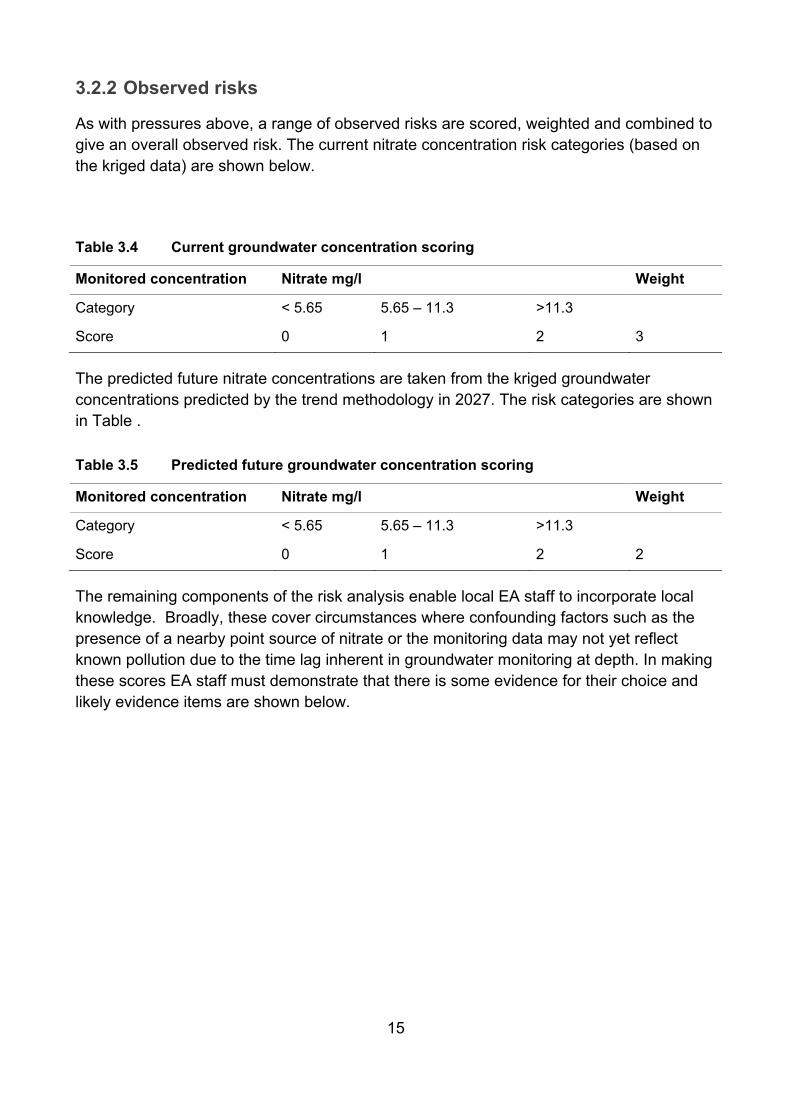
3.2.2 Observed risks

As with pressures above, a range of observed risks are scored, weighted and combined to give an overall observed risk. The current nitrate concentration risk categories (based on the kriged data) are shown below.

Table 3.4 Current groundwater concentration scoring

Monitored concentration Nitrate mg/l Weight

Category < 5.65 5.65 – 11.3 >11.3

Score 0 1 2 3

The predicted future nitrate concentrations are taken from the kriged groundwater concentrations predicted by the trend methodology in 2027. The risk categories are shown in Table .

Table 3.5 Predicted future groundwater concentration scoring

Monitored concentration Nitrate mg/l Weight

Category < 5.65 5.65 – 11.3 >11.3

Score 0 1 2 2

The remaining components of the risk analysis enable local EA staff to incorporate local knowledge. Broadly, these cover circumstances where confounding factors such as the presence of a nearby point source of nitrate or the monitoring data may not yet reflect known pollution due to the time lag inherent in groundwater monitoring at depth. In making these scores EA staff must demonstrate that there is some evidence for their choice and likely evidence items are shown below.

16

Point source pollution

Table 3.6 Point source pollution scoring

Point source risk

Groundwater concentration is unduly influenced by point source pollution Weight

Category Yes, good evidence Maybe some evidence No evidence

Score 2 1 0 -5

Identifiable point source of nitrate AND groundwater concentrations significantly higher than soil leaching concentrations.

Identifiable point source of nitrate OR groundwater concentrations significantly higher than soil leaching concentrations.

Monitoring data does not fully represent groundwater quality risks

In some cases the monitored (and kriged) nitrate concentrations derived may not fully represent relevant groundwater nitrate concentrations. In the case of the kriged concentrations; some instances may occur where a change in geology or borehole construction may extend the influence of high concentration beyond what is reasonable. Alternatively, observed nitrate concentrations may be unrealistically low for a number of possible reasons, for example:

• Deep abstractions sample older, cleaner water that is not representative of shallower groundwater nitrate such as locations where nitrate pollution has not passed through the unsaturated zone; it is on its way but has not yet been detected by monitoring

• Uncertainty in predicted nitrate values caused either by short duration of monitoring or a significant variation in the dataset.

This modification is only possible if the observed groundwater concentration is less than 11.3 mg/l. Examples of the evidence expected are shown although this is not intended to be an exhaustive list. The risk categories are shown in the table below.

17

Table 3.7 Groundwater monitoring scoring

Monitoring not fully representative

Monitored nitrate concentrations not fully representative Weight

Category Yes, good evidence

Yes, some evidence

No evidence

No, maybe some

evidence

No, good evidence

Score 2 1 0 -1 -2 3

Additional data from WFD assessments

OR

Water company has abandoned a source nearby due to high NO3

OR

Unsaturated zone > 30 m delaying nitrate measurement

OR

Aquifer is layered or the sampling is at depth

Large uncertainty in trend analysis

OR

Significant drift > 10 m delaying nitrate measure-ment

Expert view is that kriging is not sufficient in this setting

OR

large

uncertainty in trend analysis

results

Expert view is that kriging is not sufficient in this setting

AND

large uncertainty in trend analysis

results

18

Surface water interactions

If it can be identified that surface water quality is a reasonable indicator of groundwater quality then this data may be used to complement the groundwater monitoring dataset. This is only appropriate for situations where surface water and groundwater interaction is significant and surface water quality is not dominated by point source discharges. The risk categories are shown below.

Table 3.8 Use of surface water monitoring data

Surface water monitoring

Surface water quality is representative of groundwater quality Weight

Category Yes, good evidence Yes, some evidence No evidence

Score 2 1 0 1

Confident fail and >2 point source discharges in surface water.

OR

Marginal fail and <2 point source discharges in surface water.

Face value fail and <2 point source discharges in surface water.

OR

Face value pass and <2 point source discharges in surface water.

Attenuation

In some circumstances either denitrification or mixing may act to decrease the nitrate concentration in groundwater (these terms are explained in Appendix B). Where this is known to be protective of groundwater quality local staff may use the scores set out below. Nitrate leaching from agriculture must be greater than 25 mg/l and firm evidence of denitrification or mixing should be supplied. The risk categories are shown below.

19

Table 3.9 Summary of categories for de-nitrification or mixing (Area)

De-nitrification or mixing

NO3 is either de-nitrified or diluted by mixing Weighting

Category Yes, good evidence Maybe some evidence No evidence

Score 2 1 0 -1

Baseline report indicating de-nitrification or mixing. Lack of impacted groundwater monitoring sites. Local report, indicating as above.

Quantifiable source of dilution e.g. forested recharge area. Drift > 10m thick and clay rich.

3.3 Combined risk assessment The overall pressure and observed risk scores are added together and classified. Broadly, if the risk that groundwater nitrate concentration is exceeding 11.3 mg/l and agriculture is the cause, the score will be higher than 8. This will lead to potential groundwater NVZ designations.

Where the score is between 3 and 8 this suggests that either the water quality monitoring data or the agricultural loading data show high nitrate concentrations and these areas are likely to be included in potential designation areas around high risk areas dependent on the hydrogeological setting (see Section 7 on identifying land draining to polluted waters).

A low score is lower than 3 where both assessments show that nitrate concentrations were not likely to exceed 11.3 mg/l. These are generally not considered for designation and any low risk areas within a zone that are repeatedly shown to be so may be considered for removal from designation.

Areas scoring higher than 8 and currently not in an NVZ have been highlighted and presented at the workshops to understand local factors that could affect the final score for these areas. Similarly, areas of low score within existing zones have been highlighted and examined at the same workshops.

20

Table 3.4 Summary of categories for final risk score

What is the risk that groundwater nitrate is >11.3 mg/l or will be in future and agriculture is the main source?

Category High - Designate Medium

Low – No action (consider for de-designation)

Score >8 3-8 <3

4. Identifying land draining to polluted waters

Once an area of high risk has been identified from the loading and water quality monitoring above the question of where the draw the zone boundaries arises. This relies heavily on the professional judgement of our local EA staff to delineate the recharge area based on their local and scientific knowledge. In general, we have used a combination of the following:

• Coastlines

• WFD water body boundaries

• Solid and drift geology (1:50,000).

• Geological features such as faults where these are thought to provide a barrier to groundwater flow.

• Surface water feature (e.g. rivers and lakes) – these features could define a groundwater divide.

• Urban areas where there is no agricultural nitrate contribution.

• Groundwater flow lines to delineate groundwater bodies within an aquifer.

• Solution features (1:50,000 risk map) that may act as preferential pathways to the aquifer. If the rock at the surface is prone to solution features then it is important that the NVZ is extended to include this area.

These features became the “soft” boundaries for the proposed zones. Following this a software based process was used to translate these soft boundaries to individual field

21

boundaries based data from the RPA. A technical description of the process is given in Appendix C.

References Defra (2008) Description of the methodology applied in identifying waters and designating Nitrate Vulnerable Zones in England.

EA (2008) Technical Note E: The groundwater risk model and how it was used to support designation of NVZs.

Ellis, J.C., van Dijk, P.A.H. and Kinley, R.D. 1993. Codes of Practice for Data Handling – Version 1. WRc Report No. NR 3203/1/4224 for The National Rivers Authority.

Lee D., Gooday R., Seteven A., Whiteley I. (2015), “Modelling Nitrate Concentrations in Groundwater: Neap-N Nitrate leaching for 1970 and 2014”. Project ref: WT1550 Adas report for Defra and the Environment Agency.

Lerner, D.N., 2000. Guidelines for Estimating Urban Loads of Nitrogen to Groundwater. Defra Project Report, NT1845, 21 pp.

Lord, E. and Anthony, S., 2000. MAGPIE: A modelling framework for evaluating nitrate losses at national and catchment scales. Soil Use and Management, 16, 167–174.

R Core development Team (2009) R: A language and environment for statistical computing. Vienna, Austria. http://www.r-project.org

Rivett, M.O., Buss, S.R., Morgan, P., Smith, J.W.N. and Bemment, C.C. (2008). “Nitrate attenuation in groundwater: A review of biogeochemical controlling processes”. Water Research, 42, 4215–4232.

WRc. 2015. Statistical methods for Nitrate Vulnerable Zone Review 2017. WRc report reference UC10943.07 Unpublished.

WRc (2016). Review of the 43 mg/l threshold for groundwater NVZ assessment. WRc Report reference 11460.01. Unpublished

22

Appendix A

A1 What form of nitrogenous compounds do we refer to in this assessment?

Article 2 in the Nitrates Directive defines the forms of nitrogen which should be measured with the statement 'nitrogen compound: means any nitrogen-containing substance except for gaseous molecular nitrogen’

When we measure nitrogen compounds, including nitrate, we measure the compound as the nitrogen content in the sample, i.e. mgN/l. This is because for water quality monitoring purposes, we are interested in all the nitrogen compounds, and we sum these per sample to calculate losses in terms of Total Inorganic Nitrogen (TIN). This can cause confusion as the standard is given as 50 mg/l of nitrate.

Nitrogen, and therefore nitrate as N, is much lighter than nitrate because of the additional oxygen in the nitrate compound. To relate the values of TIN we use in our assessment to the Nitrates Directive standard of 50mg/l of nitrate, we must convert TIN to NO3 using the atomic weight of nitrogen (14) compared to the total weight of a nitrate molecule (62). This means that nitrogen is 22.6% of the total weight of the nitrate molecule and;

• To calculate the nitrogen content of a measurement of nitrate, you must multiply by 14/62 (22.6%)

• To calculate the weight of the nitrate molecule with a nitrogen content of x mg/l, you must

multiply this number by 4.43 ( ( )62/141

).

So 50 mg/l as NO3 = 11.3 mg/l as N or TIN

A2 Why do we use the 95th percentile to characterise water quality for NVZs?

A percentile is a summary statistic that provides information about the distribution (spread) of values in a defined population; for example, the sample data over time from a particular monitoring location. If you measured 100 values from a population, the 95%ile would be the value that was exceeded only 5% of the time. EC drinking water legislation stipulates a 95th percentile statistic. The 95th percentile is well-suited to standards where we need to be precautionary (where exceedence would risk harm to human health).

23

A3 Explanation of the Weibull method The Weibull method is an established statistical technique for ranking data and calculating robust percentile estimates.The method uses the rth ranked value within the observation dataset to provide an estimate of the 95th percentile, where r = 0.95(n + 1) and n is the number of samples. When r is not an integer, r is rounded down and up to the nearest whole number, and the corresponding concentration values for these ranks are interpolated to estimate the 95th percentile. Conservative 90% and 50% confidence intervals are calculated using binomial distribution theory, as described in the Environment Agency Codes of Practice for Data Handling (Ellis et al. 1993). A minimum of 28 and 59 samples are required to calculate the upper 50% and 90% confidence limits, respectively, so for some sites it was possible only to demonstrate with medium or low confidence that the 95th percentile was below the threshold. If the lower 90% confidence limit exceeds 11.3 mgN/l TIN as N, the monitoring point is deemed to have failed the test with high confidence; if the lower 50% confidence limit exceeds 11.3 mgN/l TIN as N, the monitoring point is deemed to have failed the test with medium confidence; if the 95th percentile estimate exceeds 11.3 mgN/l TIN as N, the monitoring point is deemed to have failed the test with low confidence.

We use the Weibull method because it’s relatively insensitive to outliers and doesn’t require data to fit a particular distribution. An example of how the Weibull estimates relate to the data is shown below in Figure A1, where:

• The dark green solid horizontal line 2009-2014 marks the Weibull 95th percentile estimate

• The green shaded band indicates the 50% confidence interval around the Weibull 95th percentile estimate and

• The wider, light green shaded band indicates the 90% confidence interval around the Weibull 95th percentile estimate.

24

Figure A1 - Current 95th percentile prediction using the Weibull method

Appendix B Nitrate attenuation and dilution An understanding of the fate of nitrate in groundwater is vital for managing risks associated with nitrate pollution. Nitrate is commonly thought of as behaving conservatively in groundwater. Although retardation of nitrate has been observed in some soils, it has not been observed in groundwater. Consequently processes that cause nitrate mass removal are the principal focus for nitrate attenuation, with denitrification generally recognised as the most significant mass removal process (Rivett et al., 2008).

As well as attenuation, nitrate concentrations in groundwater can be reduced by mixing. Usually simply by diluting groundwater with a high concentration with water of a lower concentration.

25

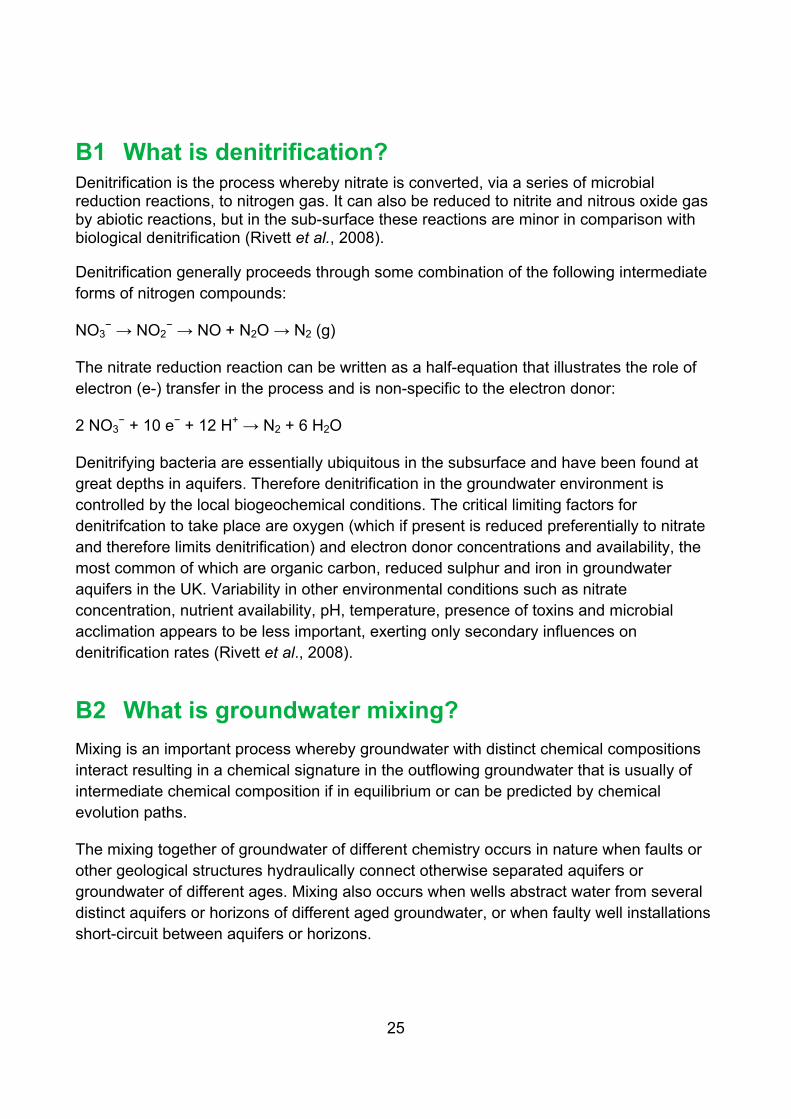
B1 What is denitrification? Denitrification is the process whereby nitrate is converted, via a series of microbial reduction reactions, to nitrogen gas. It can also be reduced to nitrite and nitrous oxide gas by abiotic reactions, but in the sub-surface these reactions are minor in comparison with biological denitrification (Rivett et al., 2008).

Denitrification generally proceeds through some combination of the following intermediate forms of nitrogen compounds:

NO3− → NO2

− → NO + N2O → N2 (g)

The nitrate reduction reaction can be written as a half-equation that illustrates the role of electron (e-) transfer in the process and is non-specific to the electron donor:

2 NO3− + 10 e− + 12 H+ → N2 + 6 H2O

Denitrifying bacteria are essentially ubiquitous in the subsurface and have been found at great depths in aquifers. Therefore denitrification in the groundwater environment is controlled by the local biogeochemical conditions. The critical limiting factors for denitrifcation to take place are oxygen (which if present is reduced preferentially to nitrate and therefore limits denitrification) and electron donor concentrations and availability, the most common of which are organic carbon, reduced sulphur and iron in groundwater aquifers in the UK. Variability in other environmental conditions such as nitrate concentration, nutrient availability, pH, temperature, presence of toxins and microbial acclimation appears to be less important, exerting only secondary influences on denitrification rates (Rivett et al., 2008).

B2 What is groundwater mixing? Mixing is an important process whereby groundwater with distinct chemical compositions interact resulting in a chemical signature in the outflowing groundwater that is usually of intermediate chemical composition if in equilibrium or can be predicted by chemical evolution paths.

The mixing together of groundwater of different chemistry occurs in nature when faults or other geological structures hydraulically connect otherwise separated aquifers or groundwater of different ages. Mixing also occurs when wells abstract water from several distinct aquifers or horizons of different aged groundwater, or when faulty well installations short-circuit between aquifers or horizons.

26

Appendix C Hard boundary conversion rule

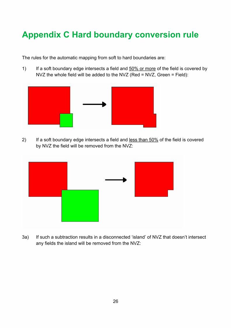
The rules for the automatic mapping from soft to hard boundaries are:

1) If a soft boundary edge intersects a field and 50% or more of the field is covered by NVZ the whole field will be added to the NVZ (Red = NVZ, Green = Field):

2) If a soft boundary edge intersects a field and less than 50% of the field is covered by NVZ the field will be removed from the NVZ:

3a) If such a subtraction results in a disconnected ‘island’ of NVZ that doesn’t intersect any fields the island will be removed from the NVZ:

27

3b) However, if an entire NVZ does not intersect any fields (i.e. it was not created by rule 4, but already existed as a distinct NVZ) then it will be kept.

3c) If an entire NVZ intersects with <50% of any field it will be removed, e.g.

field 1

N VZ field 2

4) Where the soft boundary crosses the coastline the hard boundary must follow the Mean High Water Line.

5) If a soft boundary edge does not intersect a field it will be retained where it is – edges follow field boundary, or in the absence of a field boundary, follow the soft NVZ boundary.