1

Implementing a Graph

• Implement a graph in three ways:

– Adjacency List

– Adjacency-Matrix

– Pointers/memory for each node (actually a form

of adjacency list)

Adjacency List

• List of pointers for each vertex

1 2

3 4

5

1 2 3

2

3 4

4 1

5 2 4

2

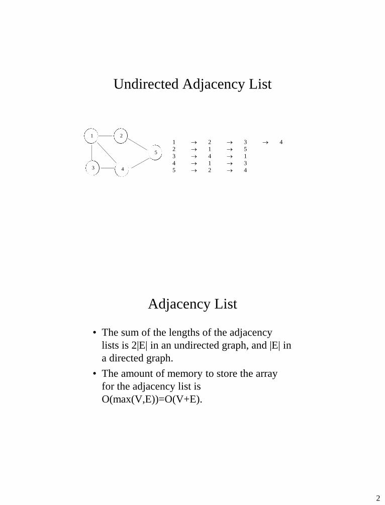
Undirected Adjacency List

1 2

3 4

5

1 2 3 4

2 1 5

3 4 1

4 1 3

5 2 4

Adjacency List

• The sum of the lengths of the adjacency

lists is 2|E| in an undirected graph, and |E| in

a directed graph.

• The amount of memory to store the array

for the adjacency list is

O(max(V,E))=O(V+E).

3

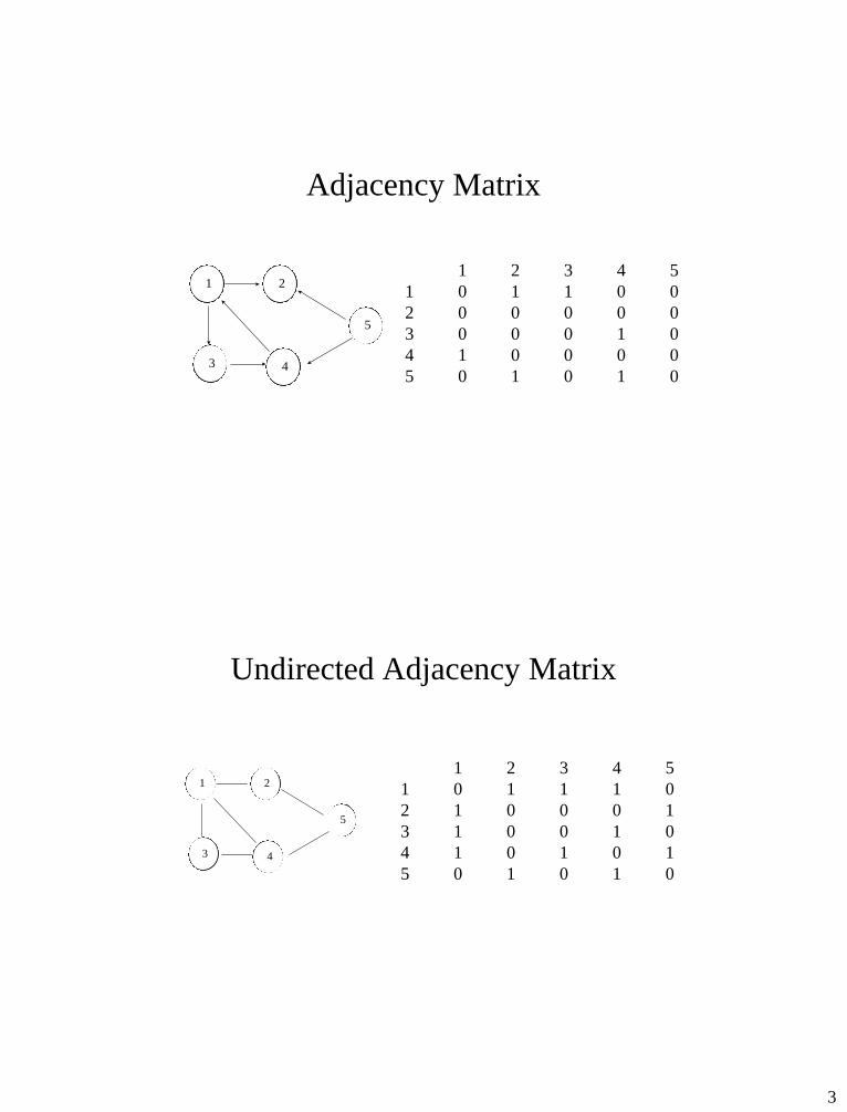
Adjacency Matrix

1 2

3 4

5

1 2 3 4 5

1 0 1 1 0 0

2 0 0 0 0 0

3 0 0 0 1 0

4 1 0 0 0 0

5 0 1 0 1 0

Undirected Adjacency Matrix

1 2

3 4

5

1 2 3 4 5

1 0 1 1 1 0

2 1 0 0 0 1

3 1 0 0 1 0

4 1 0 1 0 1

5 0 1 0 1 0

4

Adjacency Matrix vs. List?

• The matrix always uses Θ(v2) memory. Usually easier to implement and perform lookup than an adjacency list.

• Sparse graph: very few edges.

• Dense graph: lots of edges. Up to O(v2) edges if fully connected.

• The adjacency matrix is a good way to represent a weighted graph. In a weighted graph, the edges have weights associated with them. Update matrix entry to contain the weight. Weights could indicate distance, cost, etc.

Searching a Graph

• Search: The goal is to methodically explore

every vertex and every edge; perhaps to do

some processing on each.

• For the most part in our algorithms we will

assume an adjacency-list representation of

the input graph.

5

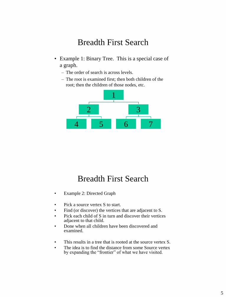
Breadth First Search

• Example 1: Binary Tree. This is a special case of

a graph.

– The order of search is across levels.

– The root is examined first; then both children of the

root; then the children of those nodes, etc.

1

2

4 5

3

6 7

Breadth First Search

• Example 2: Directed Graph

• Pick a source vertex S to start.

• Find (or discover) the vertices that are adjacent to S.

• Pick each child of S in turn and discover their vertices adjacent to that child.

• Done when all children have been discovered and examined.

• This results in a tree that is rooted at the source vertex S.

• The idea is to find the distance from some Source vertex by expanding the “frontier” of what we have visited.

6

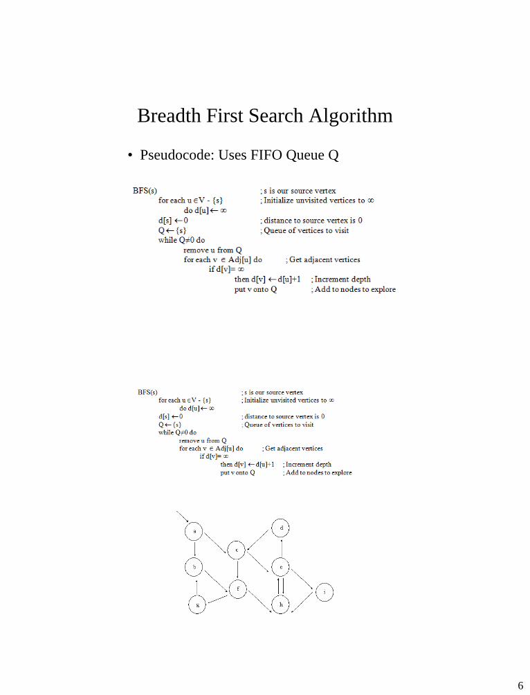
Breadth First Search Algorithm

• Pseudocode: Uses FIFO Queue Q

7

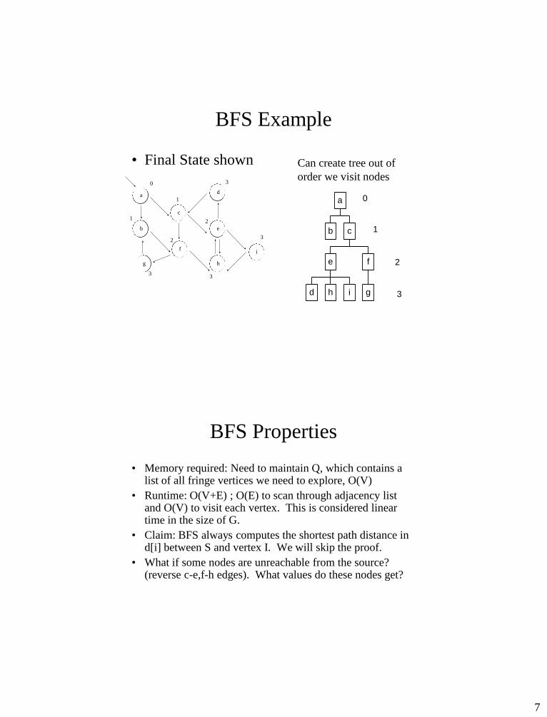
BFS Example

• Final State shown

a

b

g

c

f

d

e

h

i

0

1

1

3

2

33

2

3

0

1

2

3

b

d h i

e

g

f

c

a

Can create tree out of

order we visit nodes

BFS Properties

• Memory required: Need to maintain Q, which contains a list of all fringe vertices we need to explore, O(V)

• Runtime: O(V+E) ; O(E) to scan through adjacency list and O(V) to visit each vertex. This is considered linear time in the size of G.

• Claim: BFS always computes the shortest path distance in d[i] between S and vertex I. We will skip the proof.

• What if some nodes are unreachable from the source? (reverse c-e,f-h edges). What values do these nodes get?

8

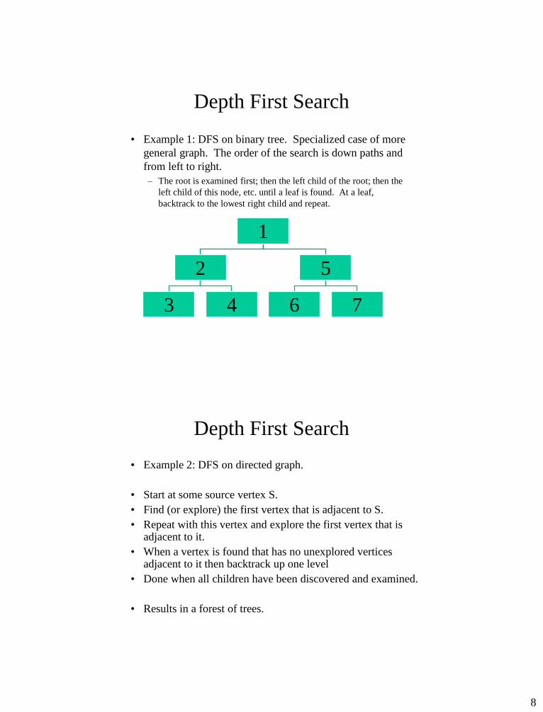
Depth First Search

• Example 1: DFS on binary tree. Specialized case of more

general graph. The order of the search is down paths and

from left to right.

– The root is examined first; then the left child of the root; then the

left child of this node, etc. until a leaf is found. At a leaf,

backtrack to the lowest right child and repeat.

1

2

3 4

5

6 7

Depth First Search

• Example 2: DFS on directed graph.

• Start at some source vertex S.

• Find (or explore) the first vertex that is adjacent to S.

• Repeat with this vertex and explore the first vertex that is adjacent to it.

• When a vertex is found that has no unexplored vertices adjacent to it then backtrack up one level

• Done when all children have been discovered and examined.

• Results in a forest of trees.

9

DFS Algorithm

• Pseudocode

DFS(s)

for each vertex uV

do color[u]White ; not visited

time1 ; time stamp

for each vertex uV

do if color[u]=White

then DFS-Visit(u,time)

DFS-Visit(u,time)

color[u] Gray ; in progress nodes

d[u] time ; d=discover time

time time+1

for each v Adj[u] do

if color[u]=White

then DFS-Visit(v,time)

color[u] Black

f[u] time time+1 ; f=finish time

10

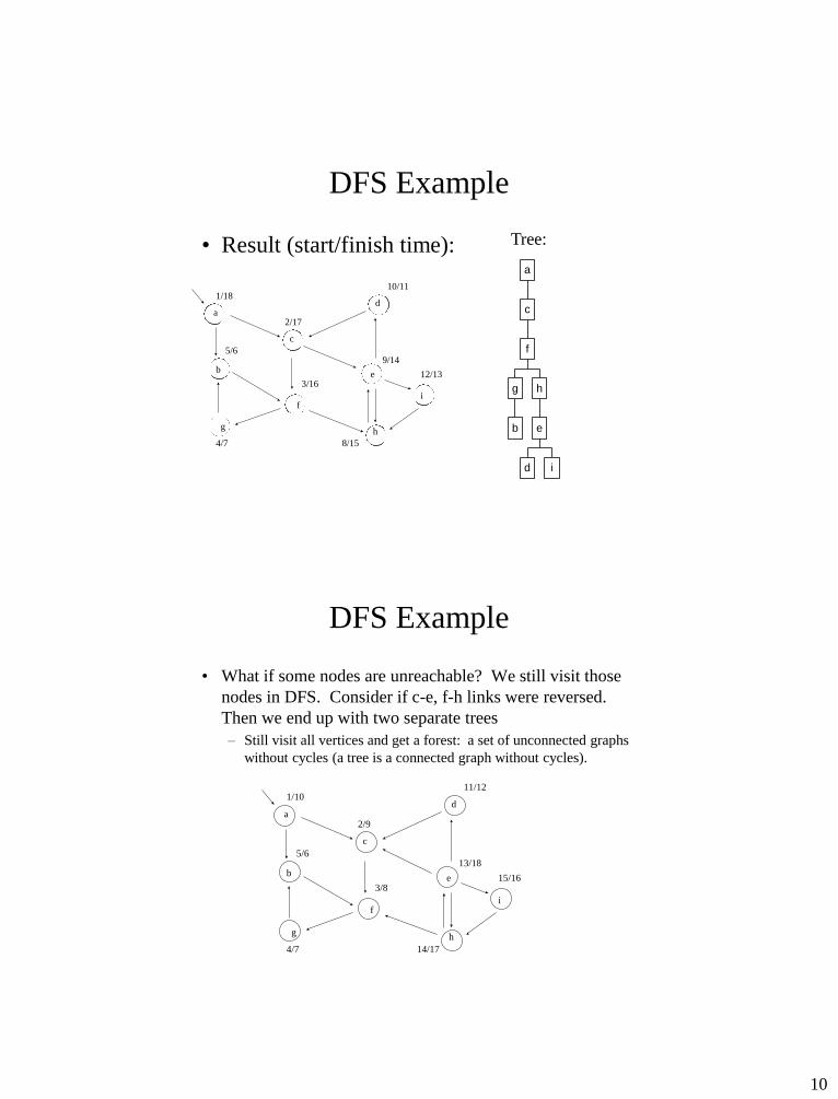
DFS Example

• Result (start/finish time):

a

c

b

g

d

e

f

h

i

1/18

2/17

3/16

4/7

5/6

8/15

9/14

10/11

12/13

Tree:

b

g

d i

e

h

f

c

a

DFS Example

• What if some nodes are unreachable? We still visit those

nodes in DFS. Consider if c-e, f-h links were reversed.

Then we end up with two separate trees

– Still visit all vertices and get a forest: a set of unconnected graphs

without cycles (a tree is a connected graph without cycles).

a

c

b

g

d

e

f

h

i

1/10

2/9

3/8

4/7

5/6

14/17

13/18

11/12

15/16

11

DFS Runtime

• O(V2) - DFS loop goes O(V) times once for each vertex (can’t be more than once, because a vertex does not stay white), and the loop over Adj runs up to V times.

• But… – The for loop in DFS-Visit looks at every element in Adj once. It is

charged once per edge for a directed graph, or twice if undirected. A small part of Adj is looked at during each recursive call but over the entire time the for loop is executed only the same number of times as the size of the adjacency list which is (E).

– Since the initial loop takes (V) time, the total runtime is (V+E).

• Note: Don’t have to track the backtracking/fringe as in BFS since this is done for us in the recursive calls and the stack. The amount of storage needed is linear in terms of the depth of the tree.

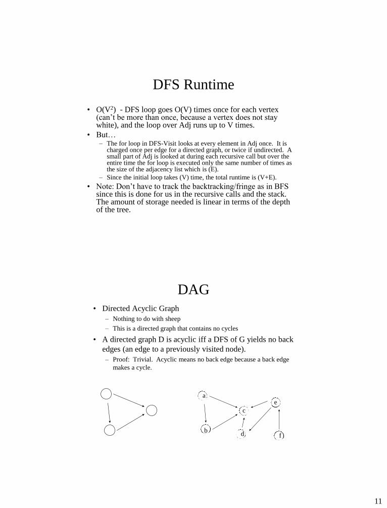
DAG • Directed Acyclic Graph

– Nothing to do with sheep

– This is a directed graph that contains no cycles

• A directed graph D is acyclic iff a DFS of G yields no back

edges (an edge to a previously visited node).

– Proof: Trivial. Acyclic means no back edge because a back edge

makes a cycle.

a

b

c

d

e

f

12

DAG

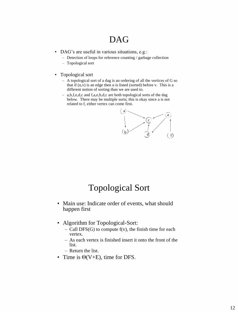
• DAG’s are useful in various situations, e.g.: – Detection of loops for reference counting / garbage collection

– Topological sort

• Topological sort – A topological sort of a dag is an ordering of all the vertices of G so

that if (u,v) is an edge then u is listed (sorted) before v. This is a different notion of sorting than we are used to.

– a,b,f,e,d,c and f,a,e,b,d,c are both topological sorts of the dag below. There may be multiple sorts; this is okay since a is not related to f, either vertex can come first.

a

b

c

d

e

f

Topological Sort

• Main use: Indicate order of events, what should happen first

• Algorithm for Topological-Sort: – Call DFS(G) to compute f(v), the finish time for each

vertex.

– As each vertex is finished insert it onto the front of the list.

– Return the list.

• Time is Θ(V+E), time for DFS.

13

Topological Sort Example

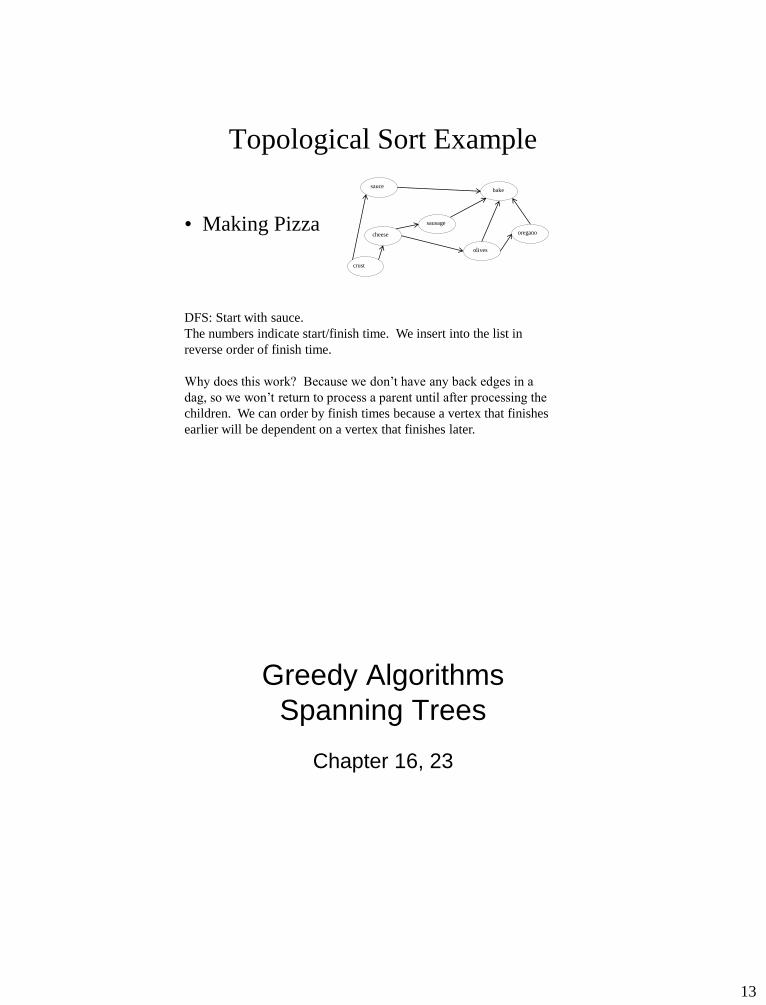
• Making Pizza

DFS: Start with sauce.

The numbers indicate start/finish time. We insert into the list in

reverse order of finish time.

Why does this work? Because we don’t have any back edges in a

dag, so we won’t return to process a parent until after processing the

children. We can order by finish times because a vertex that finishes

earlier will be dependent on a vertex that finishes later.

sauce bake

cheese

sausage

olives

oregano

crust

Greedy Algorithms

Spanning Trees

Chapter 16, 23

14

What makes a greedy algorithm?

• Feasible – Has to satisfy the problem’s constraints

• Locally Optimal – The greedy part

– Has to make the best local choice among all feasible choices available on that step

• If this local choice results in a global optimum then the problem has optimal substructure

• Irrevocable – Once a choice is made it can’t be un-done on subsequent steps of the

algorithm

• Simple examples: – Playing chess by making best move without lookahead

– Giving fewest number of coins as change

• Simple and appealing, but don’t always give the best solution

Simple Example of a Greedy

Algorithm • Consider the 0-1 knapsack problem. A thief is robbing a

store that has items 1..n. Each item is worth v[i] dollars and weighs w[i] pounds. The thief wants to take the most amount of loot but his knapsack can only hold weight W. What items should he take? – Greedy algorithm: Take as much of the most valuable item first.

Does not necessarily give optimal value!

15

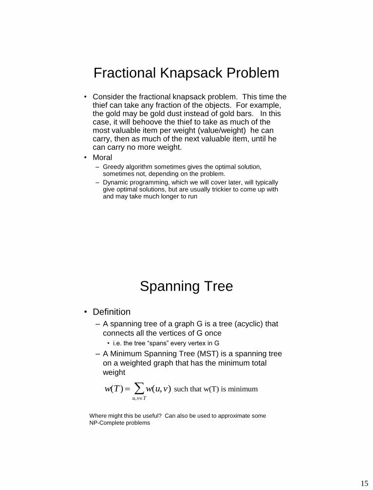
Fractional Knapsack Problem

• Consider the fractional knapsack problem. This time the thief can take any fraction of the objects. For example, the gold may be gold dust instead of gold bars. In this case, it will behoove the thief to take as much of the most valuable item per weight (value/weight) he can carry, then as much of the next valuable item, until he can carry no more weight.

• Moral – Greedy algorithm sometimes gives the optimal solution,

sometimes not, depending on the problem.

– Dynamic programming, which we will cover later, will typically give optimal solutions, but are usually trickier to come up with and may take much longer to run

Spanning Tree

• Definition

– A spanning tree of a graph G is a tree (acyclic) that

connects all the vertices of G once

• i.e. the tree “spans” every vertex in G

– A Minimum Spanning Tree (MST) is a spanning tree

on a weighted graph that has the minimum total

weight

w T w u vu v T

( ) ( , ),

such that w(T) is minimum

Where might this be useful? Can also be used to approximate some

NP-Complete problems

16

Sample MST

• Which links to make this a MST?

6

5

4

2

9

15

14

10

38

Optimal substructure: A subtree of the MST must in turn be a MST of the

nodes that it spans.

MST Claim

• Claim: Say that M is a MST

– If we remove any edge (u,v) from M then this

results in two trees, T1 and T2.

– T1 is a MST of its subgraph while T2 is a MST

of its subgraph.

– Then the MST of the entire graph is T1 + T2 +

the smallest edge between T1 and T2

– If some other edge was used, we wouldn’t

have the minimum spanning tree overall

17

Greedy Algorithm

• We can use a greedy algorithm to find the

MST.

– Two common algorithms

• Kruskal

• Prim

Kruskal’s MST Algorithm

• Idea: Greedily construct the MST

– Go through the list of edges and make a

forest that is a MST

– At each vertex, sort the edges

– Edges with smallest weights examined and

possibly added to MST before edges with

higher weights

– Edges added must be “safe edges” that do

not ruin the tree property.

18

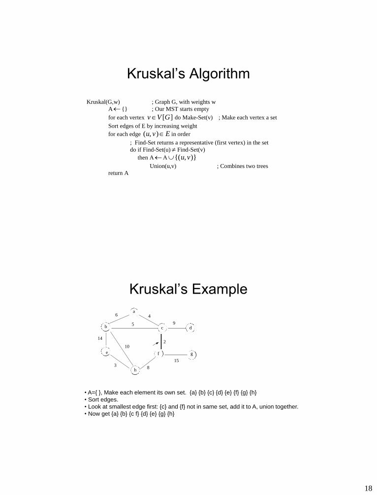
Kruskal’s Algorithm

Kruskal(G,w) ; Graph G, with weights w

A{} ; Our MST starts empty

for each vertex v V G [ ] do Make-Set(v) ; Make each vertex a set

Sort edges of E by increasing weight

for each edge ( , )u v E in order

; Find-Set returns a representative (first vertex) in the set

do if Find-Set(u) Find-Set(v)

then AA{( , )}u v

Union(u,v) ; Combines two trees

return A

Kruskal’s Example

6

5

4

2

9

15

14

10

38

a

b c d

e f g

h

• A={ }, Make each element its own set. {a} {b} {c} {d} {e} {f} {g} {h}

• Sort edges.

• Look at smallest edge first: {c} and {f} not in same set, add it to A, union together.

• Now get {a} {b} {c f} {d} {e} {g} {h}

19

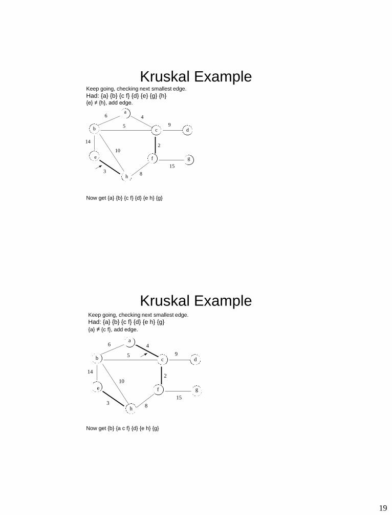
Kruskal Example Keep going, checking next smallest edge.

Had: {a} {b} {c f} {d} {e} {g} {h} {e} ≠ {h}, add edge.

6

5

4

2

9

15

14

10

38

a

b c d

e f g

h

Now get {a} {b} {c f} {d} {e h} {g}

Kruskal Example Keep going, checking next smallest edge.

Had: {a} {b} {c f} {d} {e h} {g}

{a} ≠ {c f}, add edge.

6

5

4

2

9

15

14

10

38

a

b c d

e f g

h

Now get {b} {a c f} {d} {e h} {g}

20

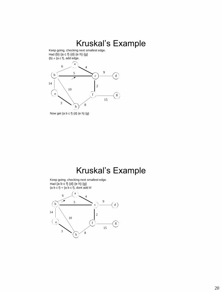
Kruskal’s Example Keep going, checking next smallest edge.

Had {b} {a c f} {d} {e h} {g} {b} {a c f}, add edge.

6

5

4

2

9

15

14

10

38

a

b c d

e f g

h

Now get {a b c f} {d} {e h} {g}

Kruskal’s Example Keep going, checking next smallest edge.

Had {a b c f} {d} {e h} {g} {a b c f} = {a b c f}, dont add it!

6

5

4

2

9

15

14

10

38

a

b c d

e f g

h

21

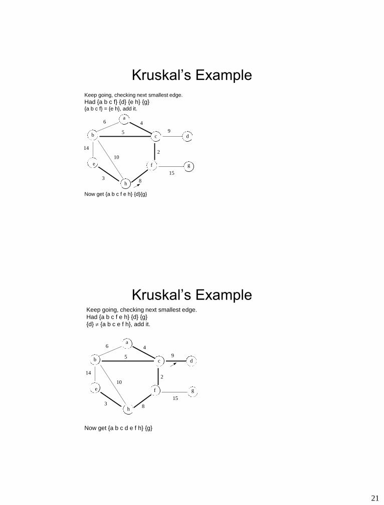
Kruskal’s Example Keep going, checking next smallest edge.

Had {a b c f} {d} {e h} {g} {a b c f} = {e h}, add it.

6

5

4

2

9

15

14

10

38

a

b c d

e f g

h

Now get {a b c f e h} {d}{g}

Kruskal’s Example Keep going, checking next smallest edge.

Had {a b c f e h} {d} {g}

{d} {a b c e f h}, add it.

6

5

4

2

9

15

14

10

38

a

b c d

e f g

h

Now get {a b c d e f h} {g}

22

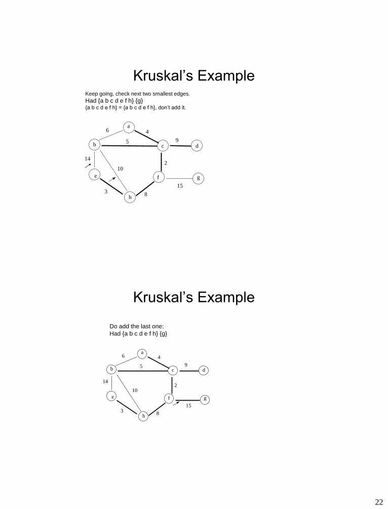
Kruskal’s Example Keep going, check next two smallest edges.

Had {a b c d e f h} {g} {a b c d e f h} = {a b c d e f h}, don’t add it.

6

5

4

2

9

15

14

10

3 8

a

b c d

e f g

h

Kruskal’s Example

Do add the last one:

Had {a b c d e f h} {g}

6

5

4

2

9

15

14

10

38

a

b c d

e f g

h

23

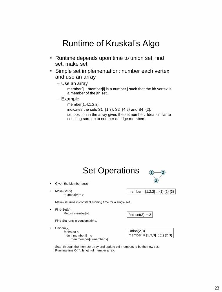
Runtime of Kruskal’s Algo

• Runtime depends upon time to union set, find set, make set

• Simple set implementation: number each vertex and use an array – Use an array

member[] : member[i] is a number j such that the ith vertex is a member of the jth set.

– Example member[1,4,1,2,2]

indicates the sets S1={1,3}, S2={4,5} and S4={2};

i.e. position in the array gives the set number. Idea similar to counting sort, up to number of edge members.

Set Operations

• Given the Member array

• Make-Set(v)

member[v] = v

Make-Set runs in constant running time for a single set.

• Find-Set(v)

Return member[v]

Find-Set runs in constant time.

• Union(u,v)

for i=1 to n

do if member[i] = u

then member[i]=member[v]

Scan through the member array and update old members to be the new set.

Running time O(n), length of member array.

1 2

3

member = [1,2,3] ; {1} {2} {3}

find-set(2) = 2

Union(2,3)

member = [1,3,3] ; {1} {2 3}

24

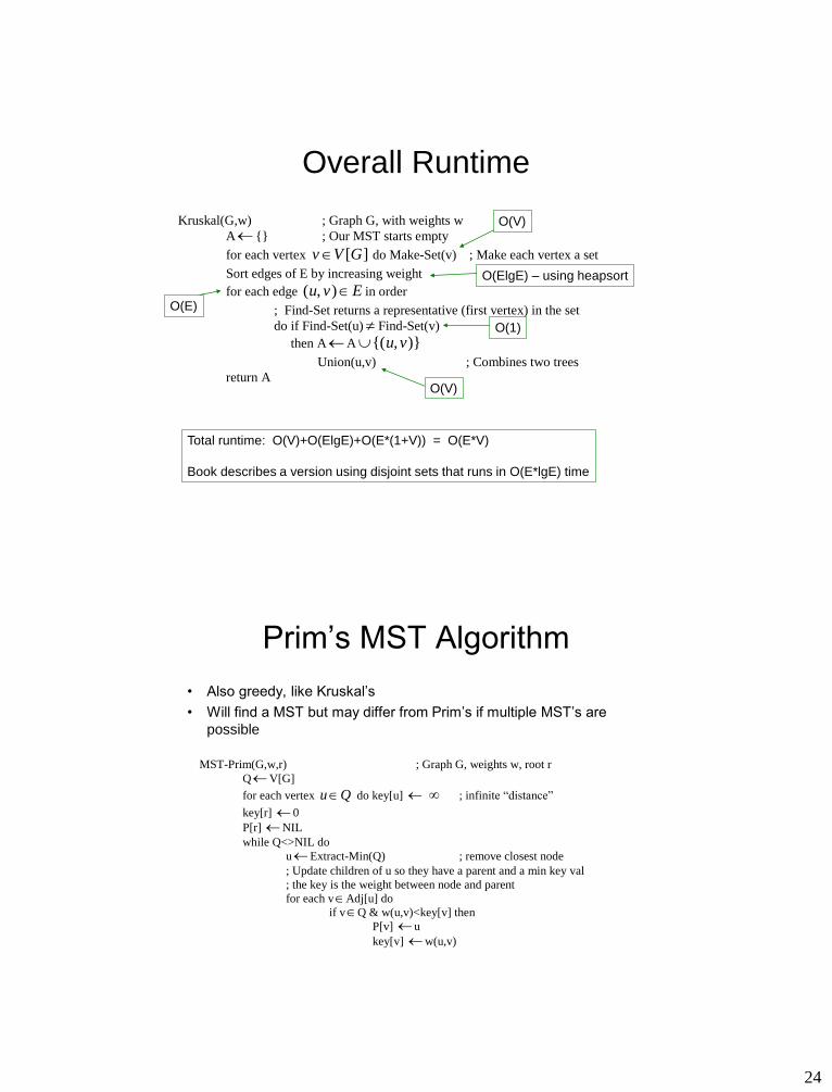
Overall Runtime

Kruskal(G,w) ; Graph G, with weights w

A{} ; Our MST starts empty

for each vertex v V G [ ] do Make-Set(v) ; Make each vertex a set

Sort edges of E by increasing weight

for each edge ( , )u v E in order

; Find-Set returns a representative (first vertex) in the set

do if Find-Set(u) Find-Set(v)

then AA{( , )}u v

Union(u,v) ; Combines two trees

return A

O(V)

O(ElgE) – using heapsort

O(1)

O(V)

Total runtime: O(V)+O(ElgE)+O(E*(1+V)) = O(E*V)

Book describes a version using disjoint sets that runs in O(E*lgE) time

O(E)

Prim’s MST Algorithm

• Also greedy, like Kruskal’s

• Will find a MST but may differ from Prim’s if multiple MST’s are

possible

MST-Prim(G,w,r) ; Graph G, weights w, root r

QV[G]

for each vertex u Q do key[u] ; infinite “distance”

key[r] 0

P[r] NIL

while Q<>NIL do

uExtract-Min(Q) ; remove closest node

; Update children of u so they have a parent and a min key val

; the key is the weight between node and parent

for each vAdj[u] do

if vQ & w(u,v)<key[v] then

P[v] u

key[v] w(u,v)

25

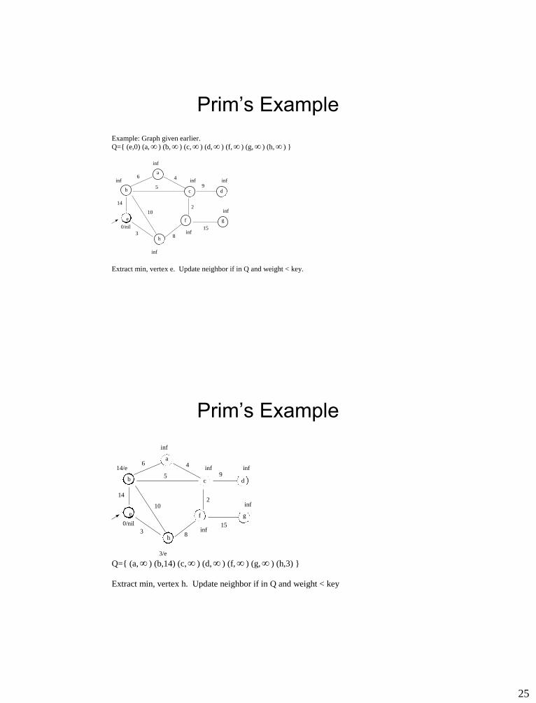
Prim’s Example

Example: Graph given earlier.

Q={ (e,0) (a, ) (b, ) (c, ) (d, ) (f, ) (g, ) (h, ) }

6

5

4

2

9

15

14

10

38

a

b c d

e f g

h

0/nil

inf

inf

inf

inf

inf

inf

inf

Extract min, vertex e. Update neighbor if in Q and weight < key.

Prim’s Example

6

5

4

2

9

15

14

10

38

a

b c d

e f g

h

0/nil

14/e

inf

3/e

inf

inf

inf

inf

Q={ (a, ) (b,14) (c, ) (d, ) (f, ) (g, ) (h,3) }

Extract min, vertex h. Update neighbor if in Q and weight < key

26

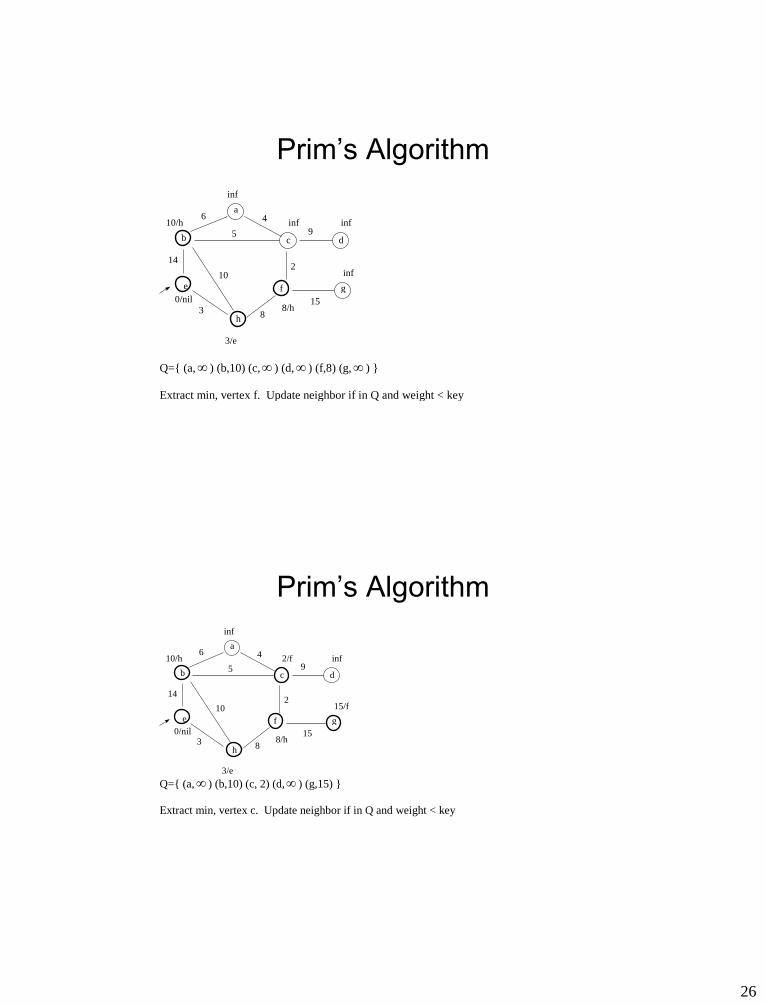
Prim’s Algorithm

6

5

4

2

9

15

14

10

38

a

b c d

e f g

h

0/nil

10/h

inf

3/e

inf

8/h

inf

inf

Q={ (a, ) (b,10) (c, ) (d, ) (f,8) (g, ) }

Extract min, vertex f. Update neighbor if in Q and weight < key

Prim’s Algorithm

6

5

4

2

9

15

14

10

38

a

b c d

e f g

h

0/nil

10/h

inf

3/e

2/f

8/h

inf

15/f

Q={ (a, ) (b,10) (c, 2) (d, ) (g,15) }

Extract min, vertex c. Update neighbor if in Q and weight < key

27

Prim’s Algorithm

6

5

4

2

9

15

14

10

3 8

a

b c d

e f g

h

0/nil

5/c

4/c

3/e

2/f

8/h

9/c

15/f

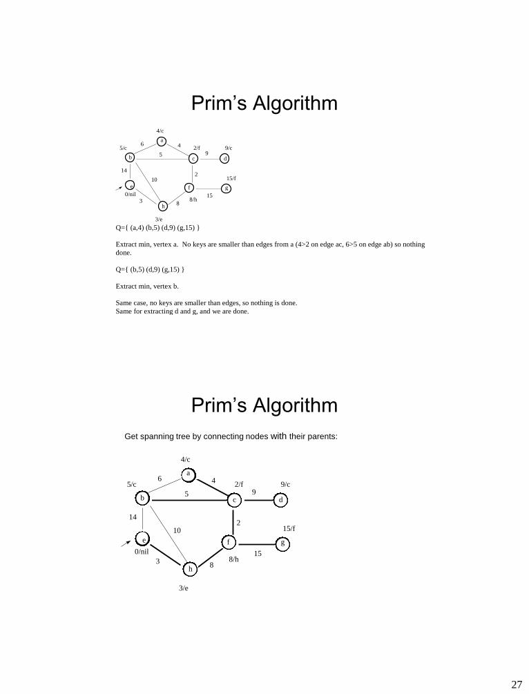
Q={ (a,4) (b,5) (d,9) (g,15) }

Extract min, vertex a. No keys are smaller than edges from a (4>2 on edge ac, 6>5 on edge ab) so nothing

done.

Q={ (b,5) (d,9) (g,15) }

Extract min, vertex b.

Same case, no keys are smaller than edges, so nothing is done.

Same for extracting d and g, and we are done.

Prim’s Algorithm

Get spanning tree by connecting nodes with their parents:

6

5

4

2

9

15

14

10

38

a

b c d

e f g

h

0/nil

5/c

4/c

3/e

2/f

8/h

9/c

15/f

28

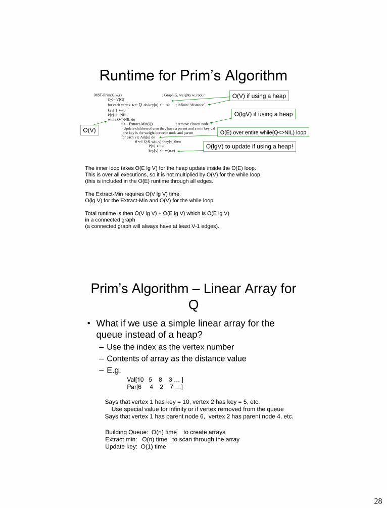
Runtime for Prim’s Algorithm MST-Prim(G,w,r) ; Graph G, weights w, root r

QV[G]

for each vertex u Q do key[u] ; infinite “distance”

key[r] 0

P[r] NIL

while Q<>NIL do

uExtract-Min(Q) ; remove closest node

; Update children of u so they have a parent and a min key val

; the key is the weight between node and parent

for each vAdj[u] do

if vQ & w(u,v)<key[v] then

P[v] u

key[v] w(u,v)

The inner loop takes O(E lg V) for the heap update inside the O(E) loop.

This is over all executions, so it is not multiplied by O(V) for the while loop

(this is included in the O(E) runtime through all edges.

The Extract-Min requires O(V lg V) time.

O(lg V) for the Extract-Min and O(V) for the while loop.

Total runtime is then O(V lg V) + O(E lg V) which is O(E lg V)

in a connected graph

(a connected graph will always have at least V-1 edges).

O(V) if using a heap

O(V)

O(lgV) if using a heap

O(E) over entire while(Q<>NIL) loop

O(lgV) to update if using a heap!

Prim’s Algorithm – Linear Array for

Q

• What if we use a simple linear array for the

queue instead of a heap?

– Use the index as the vertex number

– Contents of array as the distance value

– E.g. Val[10 5 8 3 … ]

Par[6 4 2 7 …]

Says that vertex 1 has key = 10, vertex 2 has key = 5, etc.

Use special value for infinity or if vertex removed from the queue

Says that vertex 1 has parent node 6, vertex 2 has parent node 4, etc.

Building Queue: O(n) time to create arrays

Extract min: O(n) time to scan through the array

Update key: O(1) time

29

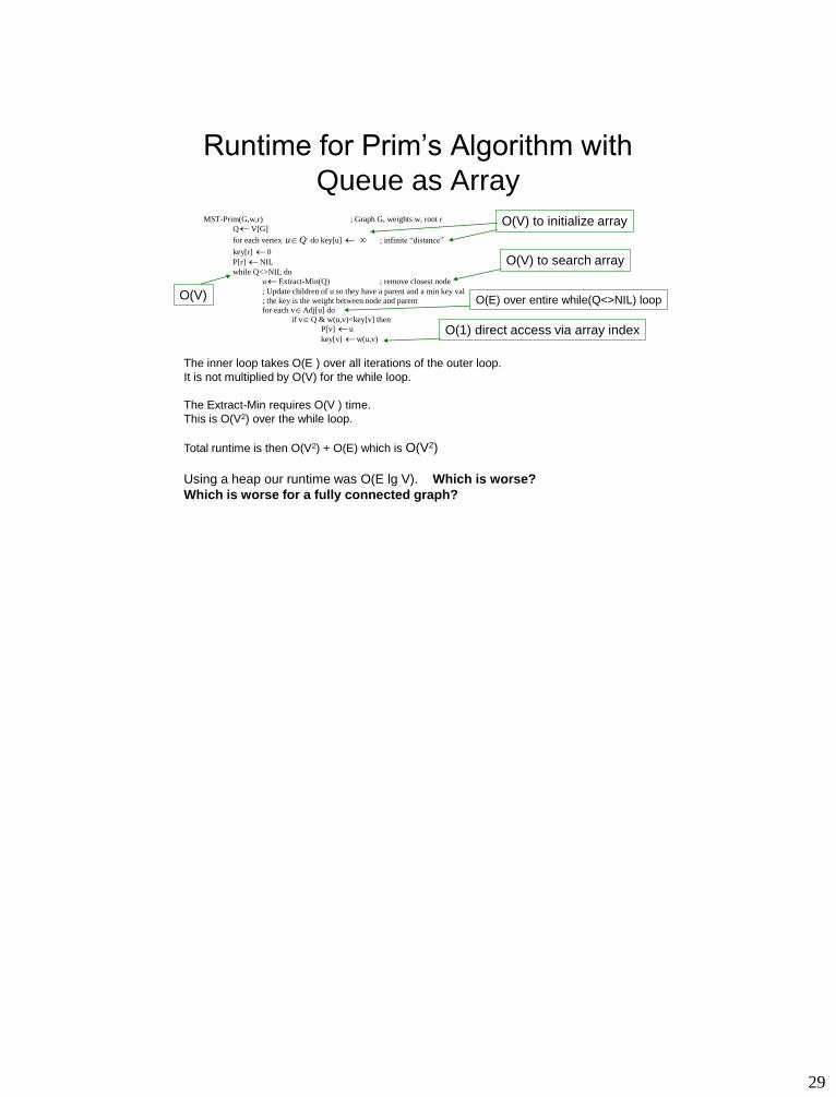
Runtime for Prim’s Algorithm with

Queue as Array MST-Prim(G,w,r) ; Graph G, weights w, root r

QV[G]

for each vertex u Q do key[u] ; infinite “distance”

key[r] 0

P[r] NIL

while Q<>NIL do

uExtract-Min(Q) ; remove closest node

; Update children of u so they have a parent and a min key val

; the key is the weight between node and parent

for each vAdj[u] do

if vQ & w(u,v)<key[v] then

P[v] u

key[v] w(u,v)

The inner loop takes O(E ) over all iterations of the outer loop.

It is not multiplied by O(V) for the while loop.

The Extract-Min requires O(V ) time.

This is O(V2) over the while loop.

Total runtime is then O(V2) + O(E) which is O(V2)

Using a heap our runtime was O(E lg V). Which is worse?

Which is worse for a fully connected graph?

O(V) to initialize array

O(V)

O(V) to search array

O(E) over entire while(Q<>NIL) loop

O(1) direct access via array index