implementing a solvency ii internal model: bayesian stochastic reserving and parameter ... ·...

Implementing a Solvency II internal model:

Bayesian stochastic reserving and

parameter estimation

Marco Pirra1, Salvatore Forte2, and Matteo Ialenti2

1 Department of Business Administration, University of CalabriaPonte Bucci cubo 3 C - 87030, Rende (CS), Italy

[email protected] Department of Statistics, Sapienza University of Roma

Viale Regina Elena, 295 - Palazzina G - 00161, Roma, Italy{Salvatore.Forte, Matteo.Ialenti}@uniroma1.it

Abstract. Often in non-life insurance claims reserves are the largestposition on the liability side of the balance sheet. Therefore, the estima-tion of adequate claims reserves for a portfolio consisting of several linesof business is relevant for every non-life insurance company. The newsolvency regulations require insurance companies to move to a market-consistent valuation of their liabilities (full balance sheet approach) andto prove the adequacy every year. Solvency II requires a view of thedistribution of expected liabilities in one year: this implies consideringthe entire distribution of the profit/loss on reserves over a one year hori-zon for the proper assessment of the reserving risk. In the present paperwe compare stochastic reserving models investigating what additionalbenefits a Bayesian approach can bring to a valuation. One of the mostinteresting is the skewness of actuarial parameters: we investigate priordistributions, which are a distinctly Bayesian feature, and analyze themost appropriate distribution shape or family for the parameters usedin the models. Prior distributions allow actuaries to incorporate externalinformation into their models, in a similar way to actuarial judgment be-ing applied to traditional spreadsheet models. We investigate the waysin which prior distributions can be used, and their impact on the pos-terior distributions through the Metropolis-Hastings algorithm. Undernew Solvency II developments insurance companies need to calculate arisk margin to cover possible shortfalls in their liability runoff. We derivean analytic formula for the risk margin which allows the comparison ofthe different proxies used in practice and we develop a flexible internalmodel that can be used for evaluating a specific risk profile. A case studyon different liability datasets investigates the influence of the dimensionon the results and gives a possible answer to some questions raised bythe International Actuarial Association. Moreover, a backtesting processcompares historical results to those produced by the current model inorder to validate both the reasonableness and the implementation of theassumptions.

Keywords. Solvency II, internal models, Bayesian stochastic methods,reserve risk, uncertainty and ranges.

2 Pirra, Forte, Ialenti

1 Introduction

The runoff of general insurance liabilities (outstanding loss liabilities) usuallytakes several years. Therefore, general insurance companies need to build ap-propriate reserves (provisions) for the runoff of the outstanding loss liabilities.These reserves need to be incessantly adjusted according to the latest informa-tion available. Under new solvency regulations, [6], general insurance companieshave to protect against possible shortfalls in these reserves adjustments withrisk bearing capital. In this spirit, this work provides a comprehensive discourseon multiperiod solvency considerations for a general insurance liability runoffand aims to give a possible answer to the questions raised by the InternationalActuarial Association, [10]. The discourse involves the description of the cost-of-capital approach in a multiperiod risk measure setting. In a cost-of-capitalapproach the insurance company needs to prove that it holds sufficient reservesfirstly to pay for the insurance liabilities (claims reserves) and secondly to paythe costs of risk bearing capital (cost-of-capital margin or risk margin). Hence,at time 0, the insurer needs to hold risk-adjusted claims reserves that comprisebest-estimate reserves for the outstanding loss liabilities and an additional mar-gin for the coverage of the cash flow generated by the cost-of-capital loadings.Such risk-adjusted claims reserves are often called a market-consistent price forthe runoff liabilities (in a marked-to-model approach), see e.g. [7], [8], [14]. Be-cause the multiperiod cost-of-capital approach is rather involved, state-of-the-artsolvency models consider a one-period measure together with a proxy for all laterperiods. Only high-quality internal models optimally reflecting the risk situationfacing the company allow insurers to assess the level of risk capital required.This importantly involves measuring and evaluating reserve risk as a part ofinsurance risks. In literature there is a wide variety of methods for stochasticreserving such as the Mack method, [13], the Bootstrap method, [4], regressionapproaches, [3], Bayesian methods, [5], etc. All these approaches are based on anultimo view, so that the uncertainty of full run-off of the liabilities is quantified.In contrast Solvency II requires the quantification of the one-year reserve risk. Inaddition the investment results, that have to be added to insurance results, arealso based on a one-year view, which means that actually many internal modelsshow an ultimo view for insurance results and the one-year view for investmentresults. So at the moment there is a discussion in academic literature and ininsurance practice, how this one-year reserve risk can be quantified. This paperfocuses on the Bayesian reserving methods and proposes a Bayesian model basedon claim numbers and average cost per claim, following the approach otulinedin [7], which can be applied in modelling reserve risk. Based on this approachwe can quantify one-year risk capital and multi-year risk capital. The results ofthe method proposed are compared with the results of the approaches proposedby CEIOPS in [2].

Bayesian stochastic reserving and parameter estimation 3

2 Bayesian Methodology

Insurance is, by nature, a very uncertain subject. Insured events occur at ran-dom times and, particularly in the field of general insurance, the amounts of theclaims are also random. The act of taking out insurance relieves the insured par-ties of some of the risk involved, passing it on to insurers, in return for a stableseries of payments. The insurer must calculate the value of premium it shouldcharge, which will be related to the total expenditure it is likely to have in ful-filling the conditions of the policies. In addition to this, the insurer must ensureit has sufficient funds, or reserves, in place to pay out claims when they occur.In order to do this, they need to learn about not only the average amount to bepaid out in any one year (which would be sufficient to determine the basic pre-mium amount), but also about the whole distribution of the aggregate claim forthe year. In the general insurance market, insurers need to use the data gatheredfrom previous years of experience to make predictions about future liabilities.The statistical analysis can be performed using Bayesian methodology, which isincreasingly common in actuarial science. While some may question the appro-priateness of prior experience in modeling, there are statisticians who believethat prior experience has a place in statistical analysis and should be formallyrecognized, even if it cannot be rigorously quantified. These statisticians arecalled Bayesians. In a Bayesian world, a modeler might start with some sense ofhow likely a parameter will take on a particular value from a prior model of theparameter, and then review the data available, changing the assessment of thislikelihood to get a posterior model of the parameter. This is possible because ofa fundamental Bayes’ theorem, which can be summarized (see Klugman, [11],for an accurate description) introducing the following definitions:

– the prior distribution is a probability distribution over the space of possibleparameter values. It is denoted π (θ) and represents our opinion concerningthe relative chances that various values of θ are the true value;

– an improper prior distribution is one for which the probabilities (or pdf) arenon-negative, but their sum (or integral) is infinite;

– the model distribution is the probability distribution for the data as col-lected, given a particular value for the parameter. Its pdf is denoted fx|θ(x|θ).Note that the expression is identical to the likelihood function, and may alsobe referred to as such;

– the joint distribution has pdf fx,Θ(x|θ)=fx|Θ(x|θ)π(θ);

– the marginal distribution of x has pdf fx(x)=∫

fx|Θ(x|θ)π(θ)dθ;

– the posterior distribution is the conditional probability distribution of theparameters given the observed data, denoted as πθ|x(θ|x);


– the predictive distribution is the conditional probability distribution of anew observation y given the data x and is denoted fY |X(y|x).

Given this background we can now state Bayes’ theorem as follows. The posteriordistribution can be computed as:

πΘ|x(θ|x) =fx|Θ(x|θ)π(θ)

∫

fx|Θ(x|θ)π(θ)dθ, (1)

while the predictive distribution can be computed as follows:

fY |X(y|x) =

∫

fY |Θ(y|θ)πΘ|X(θ|x)dθ (2)

where fY |Θ(y|θ) is the pdf of the new observation, given the parameter value.In both formulas the integrals are replaced by sums for a discrete distribution.Bayes’ theorem, therefore, provides a way to let our prior assessment evolve withadditional information, as well as to incorporate our stated uncertainty inherentin the estimation of the parameters directly into the assessment of possible fu-ture outcomes within the models framework. In this way Bayes’ theorem gives aposterior model of the parameter, rather than an estimate of the parameter it-self, as in the MLE. This principle allows for considerably more information, butalso raises the question as to which single point on the model to use to representthe parameter. To address this issue, Bayesians may consider penalty functions,which involve selecting the value of the parameter, known as a Bayesian estimateof the parameter, that incurs the least expected penalty. One benefit of Bayesianestimates is that through a judicious choice of a penalty or loss function, onecan reflect practical limitations and penalties inherent in misestimating a pa-rameter. The importance of the Bayesian approach becomes apparent when westep back and look at actuarial and related problems from a broader perspec-tive. At the heart of classical non-Bayesian statistical analysis is the conceptof asymptotically, which suggests that a large enough number of observationsfrom the same phenomenon will produce certain statistics with properties closeto some convenient models; the more observations, generally, the closer the re-sults will be to the ideal. The concept works well for repeatable experiments,such as the toss of a coin, but it requires a leap of faith when only a relativelysmall number of observations are available for an ever-changing environment.As noted above, Bayes’ theorem does not require a sufficiently large numberof observations and provides us with a useful model of the parameters, ratherthan the asymptotically normal model for MLE. However, Bayes’ theorem doesrequire a prior distribution of the parameter(s). And while it conveys how amodel would evolve as more information becomes available, it does not providea single point estimate for the parameters as does MLE. An analysts prior modelmay have a significant impact on the estimation of the parameters, particularlywhen empirical observed evidence is not plentiful. Thus, from a Bayesian pointof view, the prior model is a powerful way for past experience to be brought tobear on a current problem. Indeed, Bayes’ theorem gives a rigorous way to adapt


that prior model for emerging facts. Although a prior model can be subjective,some studies, including Rebonato,[19] require it to be, in some sense, real andverifiable so that it can be tested in the marketplace.

3 Bayesian reserving models

Stochastic reserving methods have been a keen area of research for the global ac-tuarial profession over the past decade (For reviews, see England and Verrall, [4]and Li [12]. One particular branch of stochastic methods are known as Bayesianmethods. These methods can take a variety of forms, but share a common fea-ture in that they take advantage of Bayesian statistical modelling techniques.Bayesian statistics is a branch of statistics that approaches statistical modellingfrom a slightly different perspective to classical statistics. Bayesian statisticsmakes use of two sources of information: the observed data (called the “likeli-hood”), and additional external information that may not necessarily be presentin the observed data (this is called the “prior”). Both the likelihood and theprior are formulated as probability distributions. Bayesian statistics is in con-trast to classical statistics, which is generally limited to using the observed dataonly. There are a number of benefits that Bayesian stochastic reserving modelsbring. The first benefit is that Bayesian modelling is flexible enough to buildmodels that are similar to currently used reserving models. Bayesian models caneasily incorporate GLM models, making Bayesian versions of a broad range ofstochastic reserving models possible. Under certain conditions, the Bayesian ver-sion of a model will give the same central estimate as the spreadsheet version ofthe model. This removes much of the “black box” element that many stochasticreserving models suffer from, where the stochastic model gives a result that isnot reconcilable to the result from a traditional method. Bayesian models candirectly incorporate prior information, or information that is external to the ob-served data. This is in contrast to most stochastic reserving models, which cannotincorporate information that is external to the data being analysed. Bayesianmodels provide a formal framework for integrating actuarial judgment wherean actuary does not consider the pure data alone to completely describe all ofthe information relevant to valuing the liabilities. In a sense, Bayesian modelsmay be seen as a bridge between pure stochastic models and pure deterministicmodels. They allow actuaries to enhance and expand on the strengths of existingreserving approaches, without the need to start again from scratch with a purelystochastic model. Among the reasons why Bayesian models shall be preferred toother models are the results that can be obtained and the use of prior distribu-tions. The results available are useful to understand the overall distribution ofreserves, but also the distribution of each future payment (and thus potentialvalues for each future payment). Having the full distribution of results makes itpossible to use any percentile on the distribution. From a risk margins perspec-tive, using a Bayesian model means you can use a single model to produce boththe central estimate and risk margin. Bayesian models also give a distributionof all of the stochastic parameters in the model. You can look at any or all of


these distributions, in order to check for things such as the reasonableness ofassumptions, or what the key drivers of overall volatility are. In an actuarialcontext, the prior distribution allows you to incorporate information that is notin the data. Actuaries will already be familiar with this idea, as a significantpart of any reserving exercise is the application of actuarial judgment. This canrange from ignoring particular outliers from a dataset prior to model fitting,to directly adjusting development factors where there is reason to believe thefuture experience will differ from the historical observed experience, to selectingthe prior ultimate loss ratio in a BF model. In a BF model, the model blends theactual experience as it emerges with the selected loss ratio, in a similar vein toa Bayesian model blending a prior distribution with the likelihood distribution.The external information could come from a range of sources, including:

- more extensive claims data (the particular model may be a subset of abroader class of business which may be partially useful in setting assump-tions);

- analysis performed elsewhere, such as analysis done for pricing work;- non-claims information, such as weather data (it would also be possible to

incorporate weather data directly into the model);- industry comparisons;- judgment, particularly where things such as claims management processes

or policy coverage change.

The impact on the final results of introducing a prior distribution depends on anumber of factors. These include:

- the “strength” of the prior, that is to say the lower the variance of the prioris, the greater will be the impact on the results;

- the “strength” of the likelihood/data, that is to say the higher the samplevariance/uncertainty of the likelihood, the greater the impact any prior willhave on the results. The sample variance is a measure of how dispersed thedata is;

- the number of data points, that is to say the bigger the dataset observedis, the lower the impact of the prior is. Any given prior will have a greaterimpact with only 5 data points compared to 500 data points.

There have been many papers that present a variety of Bayesian reserving mod-els. For an easy to follow introduction to using WinBUGS to build Bayesianmodels, see Scollnik, [20]. For a selection of additional Bayesian models see Nt-zoufras and Dellaportas, [18], Verrall, [21], [22], Meyers, [15], [16], [17].

4 The Bayesian Fisher Lange

In this paragraph a new Bayesian method based on claim numbers and averagecost per claim is proposed by the authors. The stochastic method presented isan extension of the traditional deterministic one and an extension of the modelproposed by the authors in GIIA, [7]. When the claim amounts paid or incurred


are divided by the relevant number of claims, an average cost per claim results.This average cost can be projected, just as were the claim amounts themselves.Then, combined with a separate projection for the number of claims, it willyield the new estimate for the ultimate loss. The reserver can also examine themovement of the claim numbers and average costs as the accident years develop,and look for significant trends or discontinuities. A fuller view of the businesscan thus be obtained, perhaps leading to adjustment of the reserving figures,or showing where further investigation is needed. The method described in thisparagraph is based on the definition of three variables that are crucial for theassessment of future payments, i.e.:

- the average cost per claim;- the proportion of claims settled;- the settlement speed.

Let Yi,j be the amount paid, properly deflated, NPi,j be the number of claimspaid and NRi,j be the number of claim reserved, being i the accident year andj the development year. The average cost per claim is defined as follows:

ACi,j =Yi,j

NPi,j

, i + j ≤ n + 1. (3)

Assume the average costs per claim follow a gamma distribution with scale equalto θAC

j and shape equal to ωACj , i.e.:

ACi,j ∼ Γ(

θACj , ωAC

j

)

1. (4)

In order to make the expected value of the average costs of development year j

a stochastic variable, the parameter θACj is assumed to be drawn from a normal

distribution as well:θAC

j ∼ N(

µ.θACj , τ.θAC

j

)

2. (5)

with mean µ.θACj and variance τ.θAC

j . Distribution (4) represents the Bayesian

Fisher Lange model, distribution (5) is a prior distribution , while µ.θACj ,τ.θAC

j

and ωACj are the hyperparameters of the model, expressed in the form of vectors

of input.Let Ratei,j represent the proportion of claims reported in the year i that arereserved in the development year j and will be paid in future different years, i.e.:

Ratei,j =

∑n−i+1k=j+1 NPi,k + NRi,n−i+1

NRi,j

, i + j ≤ n. (6)

This variable allows taking into account the possible re-opened claims and theclosed without settlement ones as well. The probability model is similar to the

1 In WinBUGS the gamma distribution with parameters a and b has the followingmoments: mean=a/b, variance=a/b2.

2 In WinBUGS the normal distribution with parameters a and b has the followingmoments: mean=a, variance=1/b.


previous one, (4). Assume that Ratei,j are drawn from a normal distribution:

Ratei,j ∼ N(

θRatej , τRate

)

, (7)

with the expected value θRatej that depends from the development year and is

drawn from a normal distribution as well:

θRatej ∼ N

(

µ.θRatej = 1, τ.θRate

)

. (8)

The hyperparameters τRate and τ.θRate are expressed in the form of costantinputs.The settlement speed νi,j represents the proportion of claims of the year i thatare paid during the development year j:

νi,j =NPi,j

∑n−i+1k=2 NPi,k + NRi,n−i+1

, i = 1, . . . n − 1; j = 2, . . . n − i + 1. (9)

The probability model follows the same structure as for (4) and (7). Assume thesettlement speeds νi,j follow a normal distribution:

νi,j ∼ N(

θνj , ων

j

)

, (10)

with the expected value being drawn from the following normal distribution:

θνj ∼ N

(

µ.θνj , τ.θν

j

)

. (11)

The hyperparameters ωνj , µ.θν

j and τ.θνj are expressed in the form of vectors of

input.The variables Ratei,j and νi,j are used for the recursive estimation of the numberof future claims paid, i.e.:

NPi,j = NRi,n−i+1 · Ratei,n−i+1 ·νi,j

∑nk=n−i+1 νi,k

, i + j > n + 1. (12)

The future payments Yi,j are obtained multiplying the number of future claimspaid and the relative average cost conveniently projected considering inflation,i.e.:

Yi,j = NPi,j · ACi,j · (1 + ir)(i+j−n−1), i + j > n + 1, (13)

where ir represents the annual inflation rate for simplicity assumed constant forthe entire reserve run-off horizon. Distribution (4), distribution (7) and distri-bution (10) represent the Bayesian Fisher Lange model, while distribution (5),distribution (8) and distribution (11) are prior distributions. The values of theinput parameters are determined on actuarial knowledge and market experience:the information relates the costs and the settlement policies a company shouldkeep traces on.


5 Solvency II and backtesting

In the Solvency II Directive framework, [6], the fair value of the technical pro-visions is defined as follows: “The value of technical provisions shall be equal tothe sum of a best estimate and a risk margin; the best estimate shall be equalto the probability-weighted average of future cash flows, taking account of thetime value of money (expected present value of future cash-flows), using therelevant risk-free interest rate term structure; the risk margin shall be such asto ensure that the value of the technical provisions is equivalent to the amountinsurance and reinsurance undertakings would be expected to require in orderto take over and meet the insurance and reinsurance obligations”. With regardto technical provisions, the act also requires insurers to have processes and pro-cedures in order to insure that best estimates and the assumptions underlyingthe calculation of the best estimates are regularly compared against experience.In case the comparison identifies systematic deviations between the experienceand the best estimate, the insurer shall make appropriate adjustments to theactuarial methods and/or the assumptions being made. The authors analysedthe fair valuation of the technical provisions in a previous paper, [7].As far as the backtesting procedures is concerned, firms that use VaR as a riskdisclosure or risk management tool are facing growing pressure from internaland external parties such as senior management, regulators, auditors, investors,creditors, and credit rating agencies to provide estimates of the accuracy of therisk models being used. Users of VaR realized early that they must carry out acost-benefit analysis with respect to the VaR implementation. A wide range ofsimplifying assumptions is usually used in VaR models (distributions of returns,historical data window defining the range of possible outcomes, etc.), and asthe number of assumptions grows, the accuracy of the VaR estimates tends todecrease. As the use of VaR extends from pure risk measurement to risk controlin areas such as VaR-based Stress Testing and capital allocation, it is essentialthat the risk numbers provide accurate information, and that someone in theorganization is accountable for producing the best possible risk estimates. In or-der to ensure the accuracy of the forecasted risk numbers, risk managers shouldregularly backtest the risk models being used, and evaluate alternative modelsif the results are not entirely satisfactory. VaR models provide a framework tomeasure risk, and if a particular model does not perform its intended task prop-erly, it should be refined or replaced, and the risk measurement process shouldcontinue. The traditional excuse given by many risk managers is that “VaR mod-els only measure risk in normal market conditions” or “VaR models make toomany wrong assumptions about market or portfolio behavior” or “VaR modelsare useless” should no longer be taken seriously, and risk managers should beaccountable to implement the best possible framework to measure risk, even if itinvolves introducing subjective judgment into the risk calculations. It is alwaysbetter to be approximately right than exactly wrong. How can the accuracy andperformance of a VaR model be assessed? In order to answer this question, wefirst need to define what we mean by “accuracy”. By accuracy, we could meannot only how well the model measures a particular percentile of or the entire


profit-and-loss distribution, but also how well the model predicts the size andfrequency of losses. Many standard backtests of VaR models compare the ac-tual portfolio losses for a given horizon vs. the estimated VaR numbers. In itssimplest form, the backtesting procedure consists of calculating the number orpercentage of times that the actual portfolio returns fall outside the VaR esti-mate, and comparing that number to the confidence level used. For example, ifthe confidence level were 95%, we would expect portfolio returns to exceed theVaR numbers on about 5% of the days. Backtesting can be as much an art as ascience. It is important to incorporate rigorous statistical tests with other visualand qualitative ones. The approach followed in the work in order to understandif the reserve predicted by the model matches the reserve held by the insurancecompany is to compare prior year development to model predictions, that is tosay compare the probability distribution and the expected value of the first di-agonal of the run-off triangle obtained by the exclusion of the last generationand the actual paid value written in the balance sheet. This type of back-testingshould be a significant part of the validation process, although the test shouldnot be limited to this.

6 Case study

This paragraphs shows the results on a sample case study. The initial data setis represented by the run-off triangle of incremental payments of an insurancecompany operating in the general liability LoB (Table 1), the triangle of thenumber of claims paid (Table 2) and the triangle of the number of claims re-served (Table 3). The aim is the analysis of the effects of the prior distributionson the outstanding claim reserve and its variability measure (coefficient of varia-tion). The input values of the parameters of the prior distributions are reportedin Table 4, Table 5 and Table 6; the choice is to set them in order to have aspecific coefficient of variation, i.e. for Ratei,j a CV=10%, for θRate

j a CV=50%,

for νi,j a CV=5%, for θνj a CV=20%, for ACi,j a CV=10%, for θAC

j a CV=10%.Table 7 reports the Bayesian Fisher Lange outstanding claim reserve assessedthrough the model described in paragraph 4 on an undiscounted basis, whileTable 8 reports the values of the discounted3 Bayesian Fisher Lange outstand-ing claim reserve, as Solvency II defines the best estimate of the claim reserveas the expected present value of future cash-flows. For comparison purposes theoutstanding claim reserve is determined through another stochastic reservingmethod, the Over Dispersed Poisson with Bootstrapping, described in [4]. Ta-ble 9 reports the ODP oustanding claim reserve on an undiscounted basis whileTable 10 reports the discounted3 ODP outstanding claim reserve. The expectedvalue is different as the deterministic methodology underlying the stochasticmodel differs as well, but the gap (around 4%) is tolerable. As far as the vari-ability is concerned the Bayesian Fisher Lange leads to higher values (6%-6.2%

3 The discounted values are obtained considering the Interest Rate Term Structure2007 given by CEIOPS in [2]. The interest rates do not consider any illiquiditypremuim.


vs. 4.5%-4.3% as it has a double level of stochasticity. The ODP has a veryhigh variability on older generations and lower values on recent generations: thisis a typical characteristic of the ODP model and in general of the chain lad-der methods. The Bayesian Fisher Lange gives homogeneous values on differentgenerations due to its bayesian nature and construction: older generations havea restricted number of datapoints to compute the posterior distribution (highvariability) and a restricted number of future values to project (low variability asthey are influenced only by recent average costs and settlement speeds); recentgenerations have a larger number of datapoints to compute the posterior distri-bution (lower variability) but many more values to project (which are influencedby more average cost and settlement speed values).Table 11 reports the values of the stability analysis on the parameter θRate

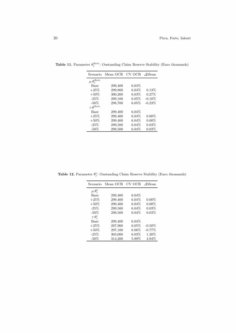
j ,

carried out varying the input parameters µ.θRatej and τ.θRate in the θRate

j priordistribution. The results show a good stability of the model, both in terms ofexpected value and standard deviation of the outstanding claim reserve: even ifthe input parameter in the prior distribution changes significantly (passing froma value of 1 to a value of 1.5) the expected value remains pretty much the same.These results demonstrate the optimal convergence of the model to the posteriordistribution, irrespective of the initial values.Table 12 reports the values of the stability analysis on the parameter θν

j , carriedout varying the input parameters µ.θν

j and τ.θνj in the θν

j prior distribution. Theresults show a good stability of the model, both in terms of expected value andstandard deviation of the outstanding claim reserve. The models tends to pro-duce identical values varying the mean of the settlement speed expected value,µ.θν

j , while seems to be slightly more sensitive varying the coefficient of varia-tion of the settlement speed expected value (that has a value of 20% in the basisscenario).Table 13 reports the values of the stability analysis on the parameter θAC

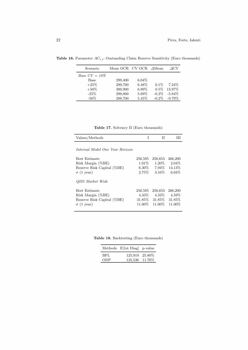
j , carried

out varying the input parameters µ.θACj and τ.θAC in the θAC

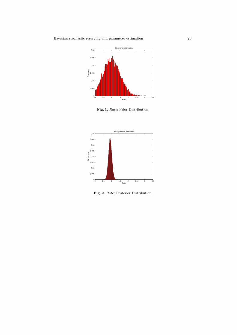
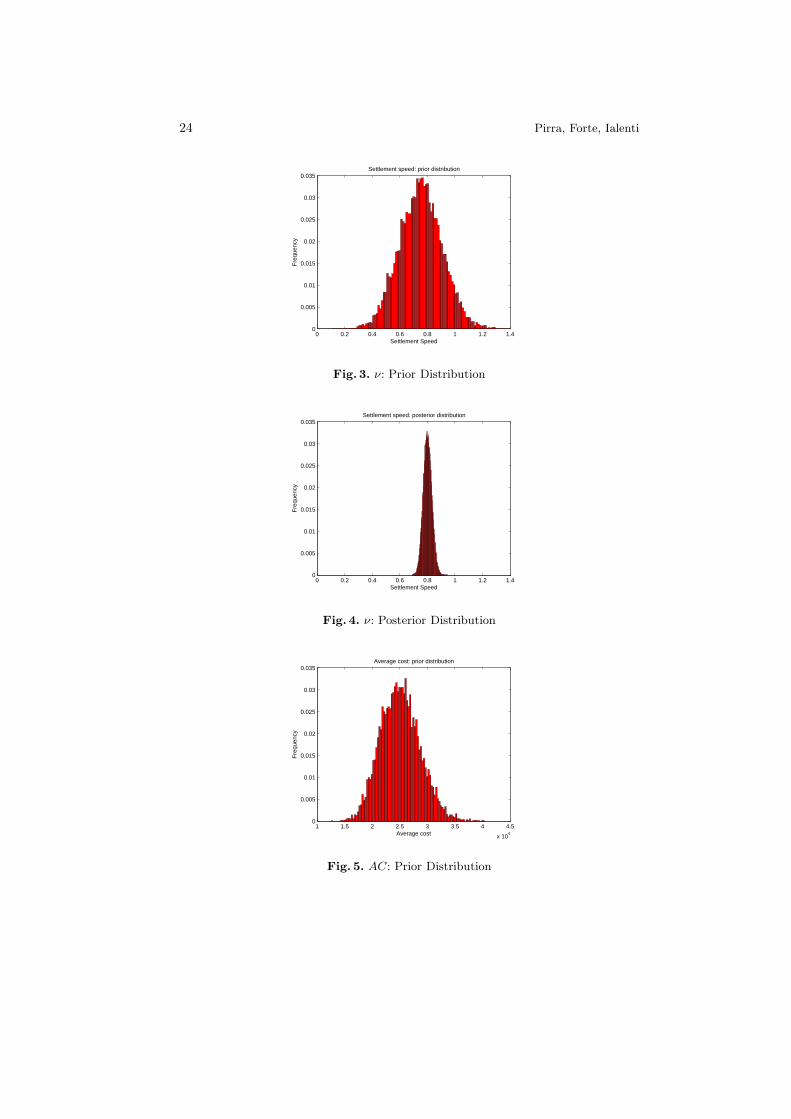
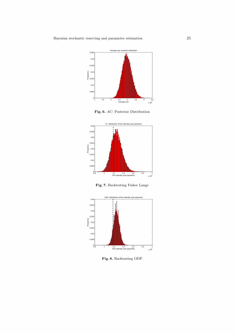
j prior distribu-tion. The results show a good stability of the model both in terms of expectedvalue and standard deviation of the outstanding claim reserve. Although the dif-ferences seem relevant, the model leads to a good convergence to the posteriordistribution: even reducing the prior average costs of a percentage equal to 50%the reduction of the expected value of the outstanding claim reserve is limitedto a 12%.Figure 1, Figure 2 and Figure 3 show the prior distribution of some selected pa-rameters while Figure 4, Figure 5 and Figure 6 their posterior distribution. Thecomparison of the figures demonstrates the optimal convergence of the model tothe posterior distributions and confirms the considerations outlined in the stabil-ity analyses: for example the AC12,9 passes from a prior expected value equal to25k to a posterior expected value equal to 29k; the Rate12,1 passes from a priorexpected value equal to 100% to a posterior expected value equal to 91.71%;ν12,2 passes from a prior expected value equal to 75% to a posterior expectedvalue equal to 80.1%.Table 14, Table 15, Table 16 report the values of some sensitivities: the analyses


are carried out varying the coefficients of variation of the model in Ratei,j , νi,j ,ACi,j .As outlined in previous paragraphs, in the Solvency II Directive framework thefair value of the technical provisions shall be equal to the sum of a best estimateand a risk margin. The different columns of Table 17 represent the different wayof calculations adopted for the best estimate assessment:

- I (method) : Merz-Wuthrich, see [13];- II (method) : ODP, see [4];- III (method) : FL Bayes, see paragraph 4.

Two different approaches for the assessment of the reserve risk capital and therisk margin are compared4:

- the “Internal Model One Year Horizon” approach, [7];- the “Standard QIS5” approach, [2];

The results show that the values both of the best estimate and the reserve riskcapital are influenced by the model chosen: appropriate selection criteria andadequate backtesting procedures play a crucial role in the assessment. As faras the QIS5 is concerned the reserve risk capital expressed as a percentage ofthe best estimate can lead to a double level of prudential estimation (the higherthe best estimate, the higher the reserve risk capital) or imprudential estimation(the lower the best estimate, the lower the riserve risk capital). The market valueof σ seems too high and it is not related to the dmension of the portfolio: somestudies (see e.g. [8]) demonstrate that the variability gets lower as the porftoliodimension gets higher. As already outlined in [8] the QIS 5 scheme leads to adouble counting of the risk margin component.As stated in previous paragraphs, Solvency II requires insurers to have processesand procedures in order to insure that best estimates, and the assumptions un-derlying the calculation of the best estimates, are regularly compared againstexperience. The approach followed in the work in order to understand if thereserve predicted by the model matches the reserve held by the insurance com-pany is to compare prior year development to model predictions, that is to saycompare the probability distribution and the expected value of the first diagonalof the run-off triangle obtained by the exclusion of the last generation and theactual paid value written in the balance sheet (in the case study the observedvalue is equal to 118,437,500 euros). Table 18 reports the results of the backtest-ing procedure: considering the expected value, the ODP model gets to a closerresult, while in terms of p-value the Bayesian Fisher Lange is to be preferred.Figure 7 and Figure 8 complete the procedure through a graphical analysis.The most appropriate backtesting methodology and the choice among differentstochastic reserving methods are still being debated in the actuarial literature.

4 See [1], [7],[8] for a more detailed description.


7 Conclusions

The results of the case study presented seem to lead to the following conclusions:

- the prior distribution allows you to incorporate information that is not inthe data. Actuaries will already be familiar with this idea, as a significantpart of any reserving exercise is the application of actuarial judgment;

- the bayesian methodology combined with the Fisher Lange model has theadvantage of explicitly taking into account the settlement and reserving poli-cies of the insurer;

- the impact on the final results of introducing a prior distribution can beadequately explained;

- the assessment of the best estimate is much more influenced by the deter-ministic methodology underlying the stochastic model rather than by theprobabilistic structure of the stochastic model itself;

- the variability measure (sigma) and the reserve risk capital are significantlyaffected by the probabilistic structure of the model and by the insurer di-mensions;

- the QIS5 standard formula states that the risk capital is a percentage of thebest estimate, different for each LoB. This approach could penalize pruden-tial insurers and could lead the management to select the methodology forthe claim reserve assessment that gives the lower result;

- the use of a unique sigma for all the insurance companies could lead to anoverestimation both of the risk capital and the risk margin. A possible solu-tion could be an entity specific sigma to be combined with the market widesigma, as proposed with the “Undertaking-Specific Parameter” approach in[2]; yet USP are not easy to compute as they require input data that are notalways available (net of reinsurance triangles) and have to be validated bythe financial authority. A simpler solution could be the consideration of anadequate size factor;

- the choice of the internal model for the reserve risk assessment has a greatimportance; that is the reason a set of validation criteria should be definedand verified through a backtesting analysis.

The results presented and the conclusions exposed depend significantly on thedatasets considered and on the insurance companies analyzed; the intention isto apply the methodologies to other insurers and verify the possibility to extendthe conclusions to other case studies.

References

1. AISAM-ACME, 2007, Study on non-life long tail liabilities. Reserve risk and riskmargin assessment under Solvency II. Available on www.amice-eu.org.

2. CEIOPS, 2010, QIS5 Technical Specifications. Available on www.ceiops.org.3. Christofides S., 1990, Regression Models based on log-incremental payments.

Claims Reserving Manual,Vol 2, Institute of Actuaries.


4. England P., Verrall R, 2002, Stochastic Claims Reserving in General Insurance.British Actuarial Journal 8, III, 443-544.

5. England P., Verrall R., 2006, Predictive Distributions of Outstanding Liabilities inGeneral Insurance. Annals of Actuarial Science: 1, 221-270.

6. European Commission, 2009, Solvency II directive (2009/138/EC). Available onec.europa.eu.

7. Forte S., Ialenti M., Pirra M., 2008, Bayesian Internal Models for the Reserve RiskAssessment, Giornale dell’ Istituto Italiano degli Attuari, Volume LXXI N.1, 39-58.

8. Forte S., Ialenti M., Pirra M., 2010, A reserve risk model for a non-life insur-ance company. Mathematical and Statistical Methods for Actuarial Sciences andFinance. Springer.

9. IAIS, 2007, Guidance paper on the structure of regulatory capital requirements,Fort Lauderdale.

10. International Actuarial Association IAA, 2009, Measurement of liabilitiesfor insurance contracts: current estimates and risk margins. Available onwww.actuaries.org.

11. Klugman S. A., Panjer H. H., Willmot G. E., 2008, Loss Models: From Data toDecisions, 3rd Edition, Wiley and Sons Edition.

12. Li J., 2006, Comparison of Stochastic Reserving Methods. Australian ActuarialJournal, volume 12, number 4.

13. Mack T., 1993, Distribution-free Calculation of the Standard Error of Chain LadderReserve Estimates. ASTIN Bulletin 23, 214-225.

14. Merz M., Wuthrich M., 2008, Modelling The Claims Development Result For Sol-vency Purposes. Casualty Actuarial Society E-Forum.

15. Meyers G., 2007, Thinking Outside the Triangle. Paper presented to the 37thASTIN Colloquium, Florida.

16. Meyers G., 2007, Estimating Predictive Distributions for Loss Reserve Models.Variance volume 1, issue 2.

17. Meyers G., 2009, Stochastic Loss Reserving with the Collective Risk Model. Vari-ance, volume 3, issue 2.

18. Ntzoufras I., Dellaportas P., 2002, Bayesian modelling of outstanding liabilitiesincorporating claim count uncertainty. North American Actuarial Journal, volume6 issue 1.

19. Rebonato R., 2007, Plight of the Fortune Tellers: Why We Need to Manage Finan-cial Risk Differently: Princeton University Press.

20. Scollnik D. P. M.,2004, Bayesian Reserving Models Inspired by Chain Ladder meth-ods and implemented using WINBUGS, Actuarial Research Clearing House 2004issue 2.

21. Verrall R., 2004, A Bayesian Generalized Linear Model for the Bornhuetter Fer-guson Method of Claims Reserving. North American Actuarial Journal, volume 8,number 3.

22. Verrall R., 2007, Obtaining Predictive Distributions for Reserves Which Incorpo-rate Expert Opinion. Variance, volume 1, issue 1.

23. Wuthrich M.V., Buhlmann H., Furrer H., 2008, Market-Consistent Actuarial Val-uation. Springer.


Table 1. Incremental Payments Triangle (Euro thousands)

Y[i,j] Development yearAccident year 0 1 2 3 4 5 6 7 8 9 10 11

1996 35,591 36,597 15,613 6,463 3,442 2,982 1,701 1,581 1,209 1,108 386 9421997 39,987 45,166 16,834 7,368 3,636 3,061 1,181 1,378 951 606 6031998 47,252 50,189 16,222 7,576 3,796 1,613 1,596 1,452 1,163 7321999 50,556 55,657 19,246 7,026 3,303 2,513 2,704 1,513 1,1242000 55,178 56,896 19,207 6,881 3,209 3,666 1,651 1,4382001 62,901 60,083 22,337 8,827 4,951 3,441 2,8672002 62,058 62,522 24,496 12,592 7,221 4,1742003 58,046 62,151 26,134 10,286 5,9262004 60,402 61,726 22,913 11,0742005 65,771 63,291 23,2882006 73,282 67,2122007 75,484


Table 2. Number of Claims Paid

NP[i,j] Development yearAccident year 0 1 2 3 4 5 6 7 8 9 10 11

1996 43,047 17,251 1,992 716 354 196 136 75 44 45 29 301997 44,350 17,154 1,882 691 267 174 70 61 40 31 261998 46,261 17,281 1,915 551 249 96 64 42 27 271999 46,304 17,045 1,835 631 211 106 85 56 392000 46,067 16,776 1,961 534 234 140 107 592001 48,970 15,757 1,996 705 347 225 2002002 46,871 15,359 2,577 930 495 3652003 42,741 15,312 2,429 957 3752004 39,141 13,435 2,391 8052005 37,952 12,652 2,0202006 38,402 13,8572007 38,244

Table 3. Number of Claims Reserved

NR[i,j] Development yearAccident year 0 1 2 3 4 5 6 7 8 9 10 11

1996 24,391 5,054 1,724 915 562 367 231 162 129 95 74 511997 23,499 4,144 1,399 667 404 237 191 137 106 79 601998 22,630 3,574 1,054 500 251 180 127 97 92 701999 21,962 3,421 1,100 500 319 229 160 117 892000 21,515 3,309 1,092 599 404 276 182 1342001 20,975 3,969 1,644 954 601 376 1872002 21,772 5,501 2,381 1,326 775 4122003 22,149 5,412 2,362 1,264 8622004 19,277 4,846 2,265 1,3192005 17,664 4,695 2,3752006 19,357 4,9202007 18,979

Table 4. Input Parameters Ratei,j

Parameter Value

τ.θRate 4τRate 100%


Table 5. Input Parameters νi,j

j µ.θνj τ.θν

j ωνj

0 1.000 25 4001 0.750 44 7112 0.100 2,500 40,0003 0.030 27,778 444,4444 0.015 111,111 1,777,7785 0.010 250,000 4,000,0006 0.005 1,000,000 16,000,0007 0.003 2,777,778 44,444,4448 0.002 6,250,000 100,000,0009 0.001 25,000,000 400,000,00010 0.001 25,000,000 400,000,00011 0.001 25,000,000 400,000,000

Table 6. Input Parameters ACi,j

j µ.θACj τ.θAC

j ωACj E[Costs]

0 100 0.01 0.05000 2,0001 100 0.01 0.02000 5,0002 100 0.01 0.01000 10,0003 100 0.01 0.00769 13,0004 100 0.01 0.00667 15,0005 100 0.01 0.00500 20,0006 100 0.01 0.00500 20,0007 100 0.01 0.00400 25,0008 100 0.01 0.00400 25,0009 100 0.01 0.00400 25,00010 100 0.01 0.00400 25,00011 100 0.01 0.00400 25,000


Table 7. Bayesian Fisher Lange Reserve Undiscounted (Euro thousands)

Year Mean StDev CV

1997 1,907 329 17.2%1998 2,047 287 14.0%1999 2,640 329 12.5%2000 4,515 499 11.0%2001 6,334 681 10.8%2002 12,700 1,337 10.5%2003 23,950 2,539 10.6%2004 30,820 3,350 10.9%2005 43,960 5,053 11.5%2006 61,910 8,056 13.0%2007 108,700 14,460 13.3%

Total 299,400 18,090 6.0%

Table 8. Bayesian Fisher Lange Reserve Discounted (Euro thousands)

Year Mean StDev CV

1997 1,821 314 17.2%1998 1,902 266 14.0%1999 2,403 299 12.4%2000 4,042 446 11.0%2001 5,595 602 10.8%2002 11,080 1,171 10.6%2003 20,790 2,217 10.7%2004 26,650 2,916 10.9%2005 38,320 4,446 11.6%2006 54,990 7,219 13.1%2007 98,620 13,280 13.5%

Total 266,200 16,400 6.2%


Table 9. ODP Reserve Undiscounted (Euro thousands)

Year Mean StDev CV

997 1,070 566 52.9%1998 1,748 707 40.4%1999 2,902 883 30.4%2000 4,347 1,029 23.7%2001 6,828 1,276 18.7%2002 9,819 1,508 15.4%2003 13,143 1,676 12.8%2004 18,236 1,951 10.7%2005 29,375 2,472 8.4%2006 58,779 3,727 6.3%2007 140,472 7,987 5.7%

Total 286,719 12,827 4.5%

Table 10. ODP Reserve Discounted (Euro thousands)

Year Mean StDev CV

1997 1,022 540 52.9%1998 1,623 654 40.3%1999 2,645 798 30.2%2000 3,902 912 23.4%2001 6,049 1,112 18.4%2002 8,597 1,296 15.1%2003 11,445 1,433 12.5%2004 15,821 1,664 10.5%2005 25,676 2,130 8.3%2006 52,305 3,285 6.3%2007 127,570 7,237 5.7%

Total 256,653 10,936 4.3%


Table 11. Parameter θRatej : Oustanding Claim Reserve Stability (Euro thousands)

Scenario Mean OCR CV OCR ∆Mean

µ.θRatej

Base 299,400 6.04%+25% 299,800 6.04% 0.13%+50% 300,200 6.03% 0.27%-25% 299,100 6.05% -0.10%-50% 298,700 6.05% -0.23%

τ.θRate

Base 299,400 6.04%+25% 299,400 6.04% 0.00%+50% 299,400 6.04% 0.00%-25% 299,500 6.04% 0.03%-50% 299,500 6.04% 0.03%

Table 12. Parameter θνj : Oustanding Claim Reserve Stability (Euro thousands)


µ.θνj

Base 299,400 6.04%+25% 299,400 6.04% 0.00%+50% 299,400 6.04% 0.00%-25% 299,500 6.04% 0.03%-50% 299,500 6.04% 0.03%τ.θν

j

Base 299,400 6.04%+25% 297,900 6.05% -0.50%+50% 297,100 6.06% -0.77%-25% 303,000 6.03% 1.20%-50% 314,200 5.99% 4.94%


Table 13. Parameter θACj : Oustanding Claim Reserve Stability (Euro thousands)


µ.θACj

Base 299,400 6.04%+25% 309,600 6.18% 3.41%+50% 317,200 6.28% 5.95%-25% 285,300 5.95% -4.71%-50% 263,000 5.86% -12.16%

τ.θACj

Base 299,400 6.04%+25% 299,600 6.07% 0.07%+50% 299,800 6.04% 0.13%-25% 299,500 6.03% 0.03%-50% 300,400 6.09% 0.33%

Table 14. Parameter Ratei,j: Oustanding Claim Reserve Sensitivity (Euro thousands)

Scenario Mean OCR CV OCR ∆Mean ∆CV

Base CV = 10%

Base 299,400 6.04%+25% 299,500 7.21% 0.0% 19.25%+50% 299,500 8.41% 0.0% 39.26%-25% 299,400 4.95% 0.0% -18.08%-50% 299,400 3.99% 0.0% -33.94%

Table 15. Parameter νi,j : Oustanding Claim Reserve Sensitivity (Euro thousands)


Base CV = 5%

Base 299,400 6.04%+25% 302,000 6.04% 0.9% -0.09%+50% 305,300 6.03% 2.0% -0.14%-25% 297,500 6.05% -0.6% 0.08%-50% 296,200 6.05% -1.1% 0.13%


Table 16. Parameter ACi,j : Oustanding Claim Reserve Sensitivity (Euro thousands)


Base CV = 10%

Base 299,400 6.04%+25% 299,700 6.48% 0.1% 7.24%+50% 300,900 6.89% 0.5% 13.97%-25% 298,800 5.69% -0.2% -5.84%-50% 298,700 5.45% -0.2% -9.79%

Table 17. Solvency II (Euro thousands)

Values/Methods I II III

Internal Model One Year Horizon

Best Estimate 256,585 256,653 266,200Risk Margin (%BE) 1.01% 1.20% 2.04%Reserve Risk Capital (%BE) 6.30% 7.94% 14.13%σ (1 year) 2.75% 3.44% 6.04%

QIS5 Market Wide

Best Estimate 256,585 256,653 266,200Risk Margin (%BE) 4.33% 4.33% 4.59%Reserve Risk Capital (%BE) 31.85% 31.85% 31.85%σ (1 year) 11.00% 11.00% 11.00%

Table 18. Backtesting (Euro thousands)

Methods E[1st Diag] p-value

BFL 125,919 25.80%ODP 125,536 11.70%


0 0.5 1 1.5 2 2.5 3 3.50

0.005

0.01

0.015

0.02

0.025

0.03

Rate

Fre

quen

cy

Rate: prior distribution

Fig. 1. Rate: Prior Distribution

0 0.5 1 1.5 2 2.5 3 3.50

0.005

0.01

0.015

0.02

0.025

0.03

0.035

0.04

Rate

Fre

quen

cy

Rate: posterior distribution

Fig. 2. Rate: Posterior Distribution


0 0.2 0.4 0.6 0.8 1 1.2 1.40

0.005

0.01

0.015

0.02

0.025

0.03

0.035

Settlement Speed

Fre

quen

cy

Settlement speed: prior distribution

Fig. 3. ν: Prior Distribution

0 0.2 0.4 0.6 0.8 1 1.2 1.40

0.005

0.01

0.015

0.02

0.025

0.03

0.035

Settlement Speed

Fre

quen

cy

Settlement speed: posterior distribution

Fig. 4. ν: Posterior Distribution

1 1.5 2 2.5 3 3.5 4 4.5

x 104

0

0.005

0.01

0.015

0.02

0.025

0.03

0.035

Average cost

Fre

quen

cy

Average cost: prior distribution

Fig. 5. AC: Prior Distribution


1 1.5 2 2.5 3 3.5 4 4.5

x 104

0

0.005

0.01

0.015

0.02

0.025

0.03

0.035

Average cost

Fre

quen

cy

Average cost: posterior distribution

Fig. 6. AC: Posterior Distribution

0.8 1 1.2 1.4 1.6 1.8 2

x 108

0

0.005

0.01

0.015

0.02

0.025

0.03

0.035

0.04

first calendar year payments

Fre

quen

cy

FL: distribution of first calendar year payments

Fig. 7. Backtesting Fisher Lange

0.8 1 1.2 1.4 1.6 1.8 2

x 108

0

0.005

0.01

0.015

0.02

0.025

0.03

0.035

0.04

first calendar year payments

Fre

quen

cy

ODP: distribution of first calendar year payments

Fig. 8. Backtesting ODP

implementing a solvency ii internal model: bayesian stochastic reserving and parameter ... ·...

Documents