implementing recommendation algorithms for decision making

Informatica Economică vol. 16, no. 3/2012 87

Implementing Recommendation Algorithms for Decision Making Processes

Paula-Ligia STANCIU, Răzvan PETRUŞEL Faculty of Economical Sciences and Business Administration,

Babeş-Bolyai University, Cluj-Napoca, Romania [email protected], [email protected]

This paper’s contribution is placed into decision-making process research area. In our previ-ous papers we showed how decision maker’s behavior can be captured in logs and how an aggregated decision data model (DDM) can be mined. We now introduce two recommenda-tion algorithms that rely on a DDM. Each algorithm aims to steer the decision maker’s ac-tions towards a fully informed decision by suggesting the next action to be performed. The first algorithm is a Greedy approach that recommends the most frequent activities performed by other decision makers. The second algorithm is inspired from A* path finding algorithm. It finds a decision sub-objective and tries to guide the decision maker on the path to it. We eval-uate these algorithms by comparing them with each other and to the classical association rules approach. It is not our intention to recommend the better decision alternative. We want to make sure the decision makers made an informed decision by correctly and completely evaluating all alternatives. This is an extended version of the paper published at IE 2012 Conference. Keywords: Decision Data Model, Recommendation Algorithm, Decision Process, Decision Path, Decision Maker Activity

Introduction Decision theory and analysis focus on

various aspects of decision making such as the overall phases of decision making, how to generate decision alternatives and which are the strategies that can be employed in choosing one of the alternatives [1]. The classic approach over the decision process is generic and focuses decision making phases like: a) knowing the context and gathering in-telligence about the decision at hand; b) de-signing an approach to solve the problem and building various decision alternatives; c) choosing and d) implementing one of the al-ternatives [2]. Compared to this research, our approach is fine-grained. We argue that the decision making process can be look at as at a sequence of actions performed by the deci-sion maker. By taking a closer look at several decision makers performing the same decision, we no-ticed that there are several common actions. But, we also found that there are a lot of ac-tions performed by just a sub-set of the deci-sion makers. We also observed that, usually, the sequence of actions is unique for each decision maker. Therefore, the decision-

making process is fuzzy and rarely per-formed in the same way by two individuals. The link with decision theory is that those fi-ne-grained actions, once made explicit, can be included in the general phases of decision making. We argue that existing high-level approaches to decision process modeling cannot precisely show why some decision makers succeed where others fail and it also cannot enable the transfer of knowledge from one individual to another. Therefore, a finer-grained approach is needed. As far as we are aware, there is no research that tries to model individual decision-making processes as a workflow. Because of the fuzziness of individual deci-sion-making, we looked at workflow man-agement and process mining because it aims to analyze existing event logs produced by process or workflow aware software (such as ERP, CRM, SCM, etc.) and to extract various models [3]. The result of process mining is a model that reflects a real life process in an enterprise [3], extracted by various algo-rithms from trace data stored in some logs. The most comprehensive collection of such algorithms can be found in ProM Framework

1

88 Informatica Economică vol. 16, no. 3/2012

(available at www.processmining.org). Our approach extracts and creates a model, but of the mental decision making process rather than of some physical process in the enter-prise. The basic assumption is that the ac-tions of a decision maker will provide an ex-ternal observer with a better understanding of a process than what the person says about that workflow. The paper is organized as follows. In the next section we provide some details about data modeling, process mining and decision mak-ing framework. The third section aims at de-scribing the formal approach for decision da-ta models and for the two recommendation algorithms considered. The fourth section of the paper is focused on the actual implemen-tation of the algorithms. In the fifth section we try to validate our assumption by using a case study and comparing the results we pro-duce with the output of association rules. In the last section we present the conclusions for the work developed during this research. 2 Related Work 2.1 Similar Approaches We have specified that the past actions of the users are important landmarks for recom-mending future actions. Our approach pre-sents two recommendation algorithms, but there are several approaches to recommenda-tion described in the specialized literature: content-based recommendation, collaborative filtering (or collaborative recommendations) and hybrid methods (that combine the first two methods) [4]. Content-based recommendation systems out-put recommendations for a certain user based on his own past preferences [4]. Content-based recommendation methods perform item recommendations by predicting the utility of items for a particular user based on how similar the item are to those he/she liked in the past. On the other hand, collaborative filtering (es-pecially using association rules) refers to processing transactions of all users for pre-diction or classification. The key characteris-tic of collaborative filtering is that it predicts the utility of items for a particular user based

on the items previously rated, purchased or executed by other like-minded users. There-fore, association rules method is comparable to our algorithms because the aggregated de-cision model we use is mined from logs that store data of the user interaction with a soft-ware. In order evaluate the recommendation algo-rithms by comparison to association rules method, we use some metrics that are based on understanding and measure of relevance. These metrics are precision and recall. When calculating these values, a higher recall (closer to 1) indicates that the algorithm re-turned most of the relevant results. High pre-cision means that the recommendation algo-rithm returns relevant operations in higher proportion than the irrelevant operations. Our goal is to demonstrate that the recommenda-tion algorithms hold better values for preci-sion and recall than association rules ap-proach. 2.2 The Decision-Making Process Mining and Modeling Framework The framework used for our research is de-picted in Fig. 1. We rely on simulation soft-ware that introduces the users to all the data needed for making some decision. The soft-ware also logs all the actions of the user dur-ing decision making (a trace of the process). The logs containing all the traces are then mined and a Decision Data Model (DDM) is extracted [1]. This is a model that deals well with fuzzy (no two decision makers perform exactly the same process), data-centric pro-cesses (as most business decisions are). The DDM can be individual (shows what an indi-vidual decision maker has done) or aggregate (shows the behavior of any number of users). We argued that the DDM (individual or ag-gregate) can be easily understood by users with no prior knowledge of it. The aggregat-ed DDM can be interpreted by an engine that, given an ongoing decision process, will pro-vide the recommendations about the next ac-tions that may be performed. The engine im-plements several recommender algorithms. One of those is covered in the remainder of this paper.


Fig. 1. The decision mining framework

To understand the recommendation algo-rithm one needs to understand the DDM. The formalism of the DDM is available in [5]. To ease the understanding, we introduce a small example in Fig. 2. The model contains two types of elements: data items and operations. The data items are either basic (e.g. period in Figure 1) created by basic operations or de-

rived (e.g. Derived Data 1 - DD1) created by deriving operations. An operation is a tuple composed of: the name of the outputted data element (e.g. DD1), the value of the output (e.g. 5000), the inputs (pairs of mathematical operations and input data elements) (e.g. (+, property_price), (-, savings)) and the time of the operation’s occurrence (e.g. t19).

Fig. 2. The Decision Data Model

3 The Formal Approach The problem of providing recommendations is to determine the “best” path through the DDM. Our problem can be mapped to a gen-eral search problem with five components [6]: S, S0, Sg, successors and cost; where:

S is a finite set of states; S0 S is the non-empty set of start states; Sg S is the non-empty set of goal states; successors is a function S → P(S) which

takes a state as input and returns another


state as output (probabilities may be used in connection with it);

cost is a value associated to moving from state s S to s´ S).

The total cost is the sum of the costs incurred by a sequence of movements from state s S0 to a state s´ Sg. A recommended strate-gy is a sequence of actions such as the total cost is minimized (or maximized under some circumstances). A particular feature of our problem is that, because we use simulation software, there are no costs for moving from a state to the next (as used in classical search problems). Instead, the notion of cost is de-rived from the notion of frequency. Definition 1: A Decision Data Model (DDM) is a tuple (D, O) with [6]: – D: the set of data elements d, D = BD DD where BD is the set of basic data ele-ments and DD is the set of derived data ele-ments; – O: the set of operations on the data ele-ments. Each operation, o is a tuple (d, v, DS, t), where:

• d DD, d is the name of the output ele-ment of the operation;

• v is the value outputted by the operation. Can be numeric or Boolean;

• DS, a set of d D, is the set of input da-ta elements of the operation.

• t T, where T is the set of timestamps at which an operation from O occurs (i.e. the time when the element d is creat-ed using o).

– D and O form a hyper-graph H = (D, O), connected and acyclic. In order to give recommendation to users in decision process, several algorithms were developed [8]. The naive one suggests the next operation by considering the absolute frequency. It has no clear target, and only aims to guide the user through the most fre-quent operations. The second algorithm as-signs priorities to operations producing a fi-nal derived data element (which are actually the decision criterions). Then, it guides the user along a path so that the operation pro-ducing a certain final data element is reached at a minimal cost. Algorithm 1: We first introduce a naive algo-

rithm which uses a Greedy approach, rec-ommending the most frequent operations that is enabled [6]. 1. Let DDMagg = (Dagg, Oagg); 2. Let op be the list with the operations in

Oagg; 3. Let no_of_occurences be the list with the

number of occurences for each op; 4. Select op with max(no_of_occurences)

and place it in Max_Occ set; 5. Compute Enabled and Executed sets; 6. For each in Executed set, search for mu-

tually exclusive operation. If found, move them from Enabled set to Executed set;

7. Compute Recommendation = Max_Occ ∩ Enabled

Algorithm 2: This approach is inspired from the A* path finding [7] algorithm [6]. 1. Create array Final with the operations

that output final data elements (fo) and their frequency (ffo);

2. Use depth-first search to calculate the di-rect paths to each element in Final and place them in Paths;

3. Evaluate each in Paths using formula Fi = (G + H) where F is the score of each path, G is the total individual cost of the operations executed in the prior states of the process and H is the total cost of the remaining operations along the selected path. The cost of an operation is calculat-ed as the sum of the frequencies of all operations divided to the frequency of that operation;

4. Current path = the element from Paths where Fi is minimal;

5. Recommendation = max frequency (Ena-bled ∩ Current Path);

6. If Recommendation = ø End Else Compute New State and go to step 3.

One can notice that there is a potential prob-lem with the Greedy approach (Algorithm 1). It can get stuck in providing the same rec-ommendation over and over if there is a high frequency operation that is repeatedly ig-nored by the user. The second algorithm adapts itself to the decision process by


changing the objective if a path with a lower cost is available to a final derived data ele-ment (decision criterion) when the user re-peatedly ignores the recommendation. Precision and recall are described in [8] and are popular metrics for evaluating infor-mation retrieval systems. Precision is defined as the ratio of relevant items selected to number of items selected [8]. Precision rep-resents the probability that a selected item is relevant. Recall, is defined as the ratio of rel-evant items selected to total number of rele-vant items available [8]. Recall represents the probability that a relevant item will be select-ed. The formulas for calculating precision P and recall R are: P = Nrs / Ns; R = Nrs

/ Nr

Where: Nrs is the number of relevant items selected; Ns is the number of the items selected;

Nr is total number of relevant items. The problem of mining association rules de-scribed in [4] can be stated as follows: Let I ={i1, i2, …, im} be a set of items. Let T = (t1, t2, …, tn) be a set of transactions (the database), where each transaction ti is a set of items ii, such that ti ⊆I. An association rule is an implication of the form, X → Y, where X ⊆ I, Y ⊆ I, and X ∩Y = . X (or Y) is a set of items, called an itemset. 4 Implementation In Fig. 1 is depicted the framework of deci-sion making process mining. After users in-teraction with decision-aware system, the de-cision logs are mined trough ProM software and an aggregated model is obtained. All the data from the aggregated model can be trans-posed in relational database tables as pre-sented in Figure 3.

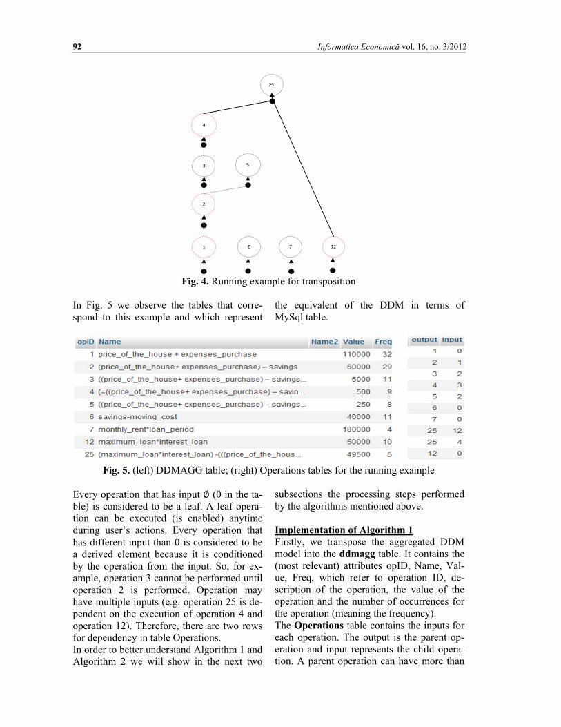
Fig. 3. The Database In the next paragraph, we will consider a running example to understand better how this transposition works. Fig. 4 is a represen-

tation of a small part of the aggregated mod-el.


1

2

5

6

3

4

127

25

Fig. 4. Running example for transposition

In Fig. 5 we observe the tables that corre-spond to this example and which represent

the equivalent of the DDM in terms of MySql table.

Fig. 5. (left) DDMAGG table; (right) Operations tables for the running example

Every operation that has input ∅ (0 in the ta-ble) is considered to be a leaf. A leaf opera-tion can be executed (is enabled) anytime during user’s actions. Every operation that has different input than 0 is considered to be a derived element because it is conditioned by the operation from the input. So, for ex-ample, operation 3 cannot be performed until operation 2 is performed. Operation may have multiple inputs (e.g. operation 25 is de-pendent on the execution of operation 4 and operation 12). Therefore, there are two rows for dependency in table Operations. In order to better understand Algorithm 1 and Algorithm 2 we will show in the next two

subsections the processing steps performed by the algorithms mentioned above. Implementation of Algorithm 1 Firstly, we transpose the aggregated DDM model into the ddmagg table. It contains the (most relevant) attributes opID, Name, Val-ue, Freq, which refer to operation ID, de-scription of the operation, the value of the operation and the number of occurrences for the operation (meaning the frequency). The Operations table contains the inputs for each operation. The output is the parent op-eration and input represents the child opera-tion. A parent operation can have more than


1 child. It can be queried so that all inputs of an operation can be extracted. The Input_string table captures the last op-eration performed by the user and its details like the value of the operation and the PIID (Process Instance ID) of the user who per-forms the action. Trace table focuses on operations performed by all users. An important attribute of trace table is Name2.This attribute stores content

of Name attribute in a different form: every operator +, -, *, /, every =, ‘ ’, (, ) sign is re-placed with “#”. We used this transformation to have uniform expression for each opera-tion so that the inputs can be easily extracted no matter how complex the expression is. Every input string received from the web ap-plication is stored in table trace while the last string is captured in input_string.

Fig. 6. The Architecture of the recommender system

In fact, as it can be observed in Fig. 6, the application focuses on creating recommenda-tion for end-users in real time. In order to understand the user’s perspective over the recommendation algorithms we in-troduce in Figure 7 the system’s user inter-face. There are three main parts in this inter-face. Section A refers to operations per-formed by the user in the current work ses-sion. Section B aims to describe the outputs of the recommendation algorithms and sec-tion C consists of the basic elements that are the base of the decision (textboxes that con-tain particular data for the context of renting or buying a certain house). In part A one can see that the user first per-formed the operation: expens-

es_for_purchasing_house + price_of_the_house=, which is operation1. It continues with (expens-es_for_purchasing_house + price_of_the_house=) - savings= , which is operation 2. Afterwards, the user chooses to perform ((expenses_for_purchasing_house + price_of_the_house=) - savings=) * inter-est_per_year_loan=, that is operation 3. In part B one can see that the Greedy algo-rithm recommends at this point two opera-tions: savings - moving_cost and month-ly_income – monthly_rent_for_house be-cause they have the same maximum frequen-cy. For now, the user can pick any recom-mendations out of these or perform another operation as he agrees.


Fig. 7. Running example 1– performing operations and receiving recommendations on the web application

In the next part of this section we will ex-plain how those recommendations are pro-duced. First of all, the input string opID is searched in ddmagg table. After the recogni-tion of the opID, some SQL queries are per-

formed. In order to achieve the goal which is offering recommendation for end-users some steps are followed. For a graphical overview of the steps described below, we will use the activity diagram in Figure 8.

Fig. 8. Activities diagram for algorithm 1


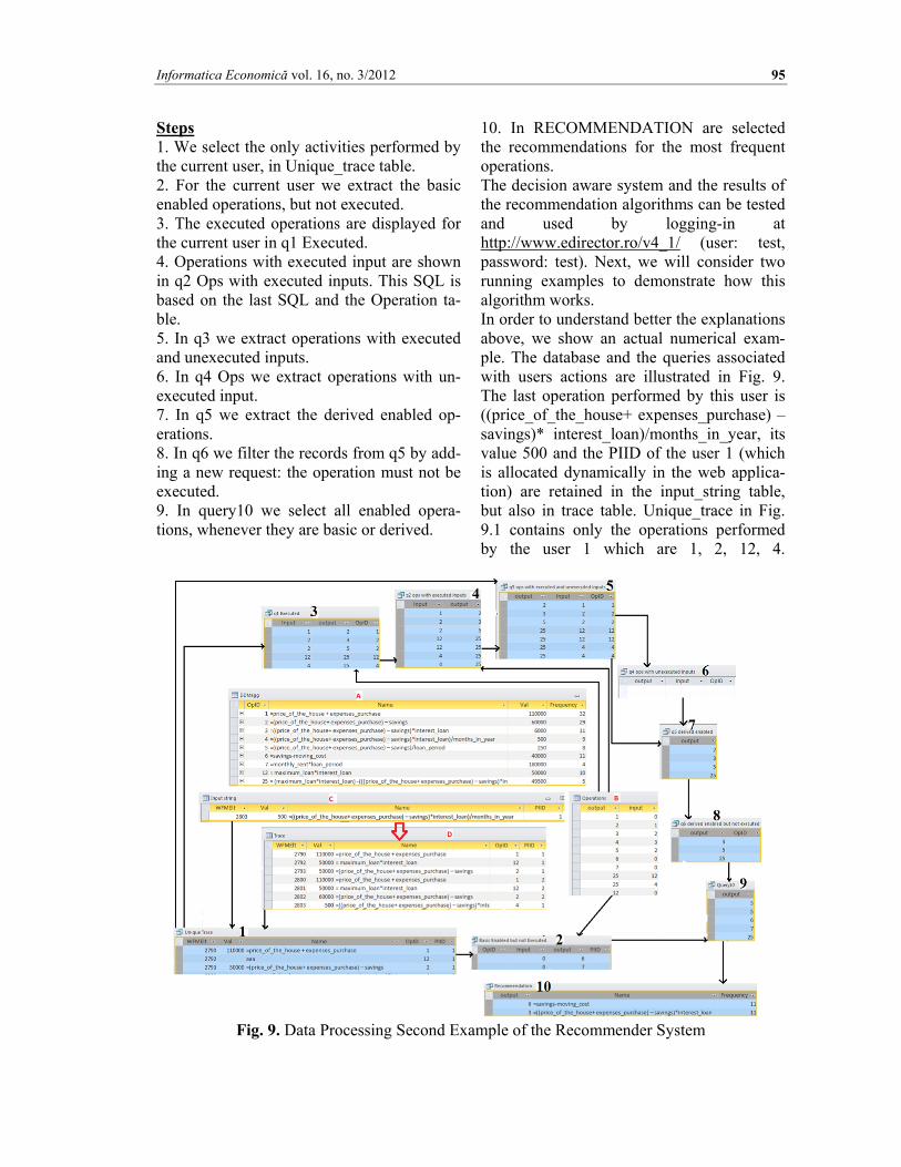
Steps 1. We select the only activities performed by the current user, in Unique_trace table. 2. For the current user we extract the basic enabled operations, but not executed. 3. The executed operations are displayed for the current user in q1 Executed. 4. Operations with executed input are shown in q2 Ops with executed inputs. This SQL is based on the last SQL and the Operation ta-ble. 5. In q3 we extract operations with executed and unexecuted inputs. 6. In q4 Ops we extract operations with un-executed input. 7. In q5 we extract the derived enabled op-erations. 8. In q6 we filter the records from q5 by add-ing a new request: the operation must not be executed. 9. In query10 we select all enabled opera-tions, whenever they are basic or derived.

10. In RECOMMENDATION are selected the recommendations for the most frequent operations. The decision aware system and the results of the recommendation algorithms can be tested and used by logging-in at http://www.edirector.ro/v4_1/ (user: test, password: test). Next, we will consider two running examples to demonstrate how this algorithm works. In order to understand better the explanations above, we show an actual numerical exam-ple. The database and the queries associated with users actions are illustrated in Fig. 9. The last operation performed by this user is ((price_of_the_house+ expenses_purchase) – savings)* interest_loan)/months_in_year, its value 500 and the PIID of the user 1 (which is allocated dynamically in the web applica-tion) are retained in the input_string table, but also in trace table. Unique_trace in Fig. 9.1 contains only the operations performed by the user 1 which are 1, 2, 12, 4.

Fig. 9. Data Processing Second Example of the Recommender System


The next step indicated in Fig. 9.2 is to iden-tify the operations which are basic enabled, but not executed. These are operations 6 and 7, because they have 0 as input. In other words these are leaf elements for the DDM. Furthermore, we are interested in details re-lated to the executed operations. So, (in 3) we observe operation 2 appears as input, but also as output and that it has two parents 3 and 5. Moreover operation 25 has two inputs: 4 and 12. It is very important to understand that the recommendation algorithm will recommend an operation only if all its children operations are already executed. At (4) the operations with executed input are listed: 2, 3, 5, 25. In this example there are no operations with unexecuted inputs (Fig. 9.6), so in Fig. 9.5 the list of operations with executed and un-executed operations remains 2, 3, 5, 25. If we consider the hypothesis of a user, named user X who performs the exact operations as user 1 except the last one is not done (meaning operation 4), than in this case the list of oper-ation with unexecuted input would contain 25. This element would have an executed in-put element (12) and an unexecuted input el-

ement(4).In this case (Fig. 9.7) the derived enabled would display only 2, 3, 5.We have ended this assumption and return to the initial example. So (Fig. 9.7) is illustrated the de-rived enabled operations which are: 2, 3, 5, 25. Some of these derived enabled operations might already be executed. 2 is the operation in this terms. So, (Fig. 9.8) those operations that are enabled, but not executed are: 3, 5, 25. Now an union is necessary between basic and derived enabled but not executed (Fig. 9.9).The list is 3, 5, 6, 7, 25.To verify the re-sult union the results from (2) and (8). There is only one step to be done to obtain the rec-ommendation for this example. In Fig. 9.10 we select the operation from 9 top 1 in a de-scending order with frequency criteria. The result is operation 6 and 3 with the same fre-quency, 11. Algorithm 2 We use the following tables as input for this second recommendation algorithm: ddmagg, operations, trace, input_string. Ddmagg and operations table are presented in Fig. 5 and the last two tables are the ones below.

Fig. 10. Running Example Data for Algorithm 2

PRELIMINARY STEPS: At first, the user has to perform an operation which is inserted in the input_string and trace table. Every operation in trace table has the attribute opID. So for every operation that was performed by a certain user we have to find the correspondent in table ddmagg in order to see if the same operation was per-formed earlier by other user. If the result is positive, the attribute trace.opID for the last row is updated from default 0 to the opID

found for the same operation name by exe-cuting the sql command: "update trace set opID='$opID_ddmagg', PIID='$piid' where Name='$name'". Secondly, we select only those operations from trace that were executed by the current user, in unique_trace. In our scenario, the PI-ID of the user is 1, so the unique_trace will contain all the operations performed by this user. Remember that in trace table the con-


tent refers to all users and all operations. The unique_trace table is described in Fig. 11.

Fig. 11. Table unique_trace which contains the operations made by the current user

Steps: 1. We create final array which contains all fi-nal operations and their inputs. The SQL command which illustrates the final opera-tions is: "SELECT operations.output, opera-tions.input FROM operations LEFT JOIN operations AS operations_1 ON opera-tions.output = operations_1.input WHERE

(((operations_1.output) Is Null))". This sql returns only those operations that are only output and not input for other operations. The result of this SQL is described as follows: output 5, 6, 7, 25, 25; input: 2, 0, 0, 12, 4. For every element in output list exists an el-ement in the input list on the same position. The result is viable for the running example considered. 2. For every final operation in final, meaning for 5, 6, 7, 25 we have to perform depth search algorithm in order to find the path(s) to them. We use the DDM in Fig. 4 for the running example. The graphical presentation in Fig. 12 will be very useful in understanding the results of the depth search algorithm.

Fig. 12. The table of all paths for the running

example

The next subsection describes Depth-First Search Algorithm in order to understand how table path was created: Input: Operations table (in the theoretical approach this is a graph G and a vertex v of G). Output: Path table (in the theoretical ap-proach this is a labeling of the edges in the connected component of v as discovery edg-es and back edges) procedure DFS(G,v): label v as explored for all edges e in G.incidentEdges(v) do if edge e is unexplored then w ← G.opposite(v,e) if vertex w is unexplored then label e as a discovery edge recursively call DFS(G,w) else label e as a back edge 3. The depth search algorithm will return for final element 5 the list 1, 2, 5; for final 6, the list 6; for final 7, the list 7; for final 25 two different lists: 12, 25 and 1, 2, 3, 4, 25. We create the path table in Fig. 12 in 2 essential steps. At first we count the number of col-umns then we create a matrix which contains on each column the path to follow to get to the final operation. The table path presented in Fig. 12 is such a matrix (we used -1 value to fill the empty cells). Further, we concen-trate our attention on each of these columns. 4. Afterwards, the sum of frequencies must be calculated in order to find out the cost of every operation that is considered in ddmagg table. Therefore, by using a SQL statement, the sum is returned. In our case, the total sum of frequencies is 113 as indicated in Fig. 13. Hence, the operation cost for every operation is calculated as:


, 1, … ,

where: n is the total number of operations, sumoffreq is the total sum of frequencies in ddmagg and opfreqi is the frequency for eve-ry operation in ddmagg. In Fig. 13, we show the costs for every op-eration. We need the opcost to calculate the F function as inspired from the A* algorithm.

Fig. 13. Operation costs

5. Hence, we start by calculating the G and H function for every column in path. We have to perform recursive calculations for every path. In our case there are 7 paths to take into consideration. g function receives as a parameter every column from path and calculates for every path the cost F as G+H. Afterwards the algorithm will recommend the next operation to be performed from the path with the lowest cost. 6. At first, we want to take all opID of operations that are considered to be in the standard path of the goal, and to calculate the cost F_all of this path without any deviation. Therefore all operation cost for every column in path is sumed up. For example, for our last column in path, which contains 1, 2, 3, 4, 25 elements (while others are equal to -1) with the costs 3.53, 3.9, 10.27, 12.56, 22.6; the total cost calculated is 52.86. This was the straight-up way to calculate the path cost. What if there are multiple operations performed outside the path? How does this aspect affect our approach? Well, it adds suplimentary cost and so G is increased. Hence, if G becomes so large that by calculating F=G+H, the sum will exceed the F of another path from which we haven’t

performed any operation, then we have to give up the initial path and recommend performing operations from the latter. 7. Therefore, we identify the elements that are executed from the path and name them G_executed_inside_path. In our case operations 1, 2 and 4 were performed with costs 3.53, 3.9 and 12.56. The total cost for these elements is 19.99. 8.If there are operations executed outside the path, we name this as G_executed_outside_path. For path c7 in our example, we identify that op 12 is executed outside the path and its cost is 11.3. We will see if this operation will not change our direction towars another path that has a lower cost in being performed (although it contains or not operation 12). As a result, G=19.99+11.3=31.29 (for path c7). 9. Furthermore, we concentrate on those operations that are inside the path, but weren’t executed until now. We name this operations as H_not_executed_from_path. For path c7, H_not_executed_from_path consists of 3 and 25 with opCost 10.27 and 22.6. So in order to achieve the goal of executing all operations from path c7 the sum 10.27+22.6=32.87 must be added. 10. So, F is the cost of all operations that are executed along the path plus all operations that are executed outside the path. In other words:

∩ ∪ ∖.

For path c7, F= 31.29 + 32.87 = 64.16, while if no deviations were made from this path, i.e. no other operations were performed, then the F would be equal to 52.86.

Fig. 14. F function

11. After, calculating the F values for all paths, we observe path c1 is the least


expensive path of all. We remind that ideal path c1 means performing 1, 2, 5 operations. In our running example it is intuitive that operation 5 must be performed because 1 and 2 have already been performed as unique_trace indicates and operation 5 is the next father operation. Anyway, our real path c1 involves 1, 2, 4, 12 operations until now. As the calculations indicate real path c1 owns the lowest cost of all. Therefore, we have to analyze which is the next operation from ideal path that is next to be performed. At first we indicate all operations that weren’t executed inside the path. Afterwards we have to indicate which are the name of the operations that weren’t executed. Hence, an inner join is required between rec and ddmagg as follows:

$sqlp="SELECT ddmagg.Name, rec.col, ddmagg.Freq FROM rec INNER JOIN ddmagg ON rec.col = ddmagg.opID". From the entire list of operations the algorithm selects only those operations with the highest level of frequency. The sqls related to this are: $sqlr="SELECT ddmagg.Name, rec.col, ddmagg.Freq FROM rec INNER JOIN ddmagg ON rec.col = ddmagg.opID ORDER BY ddmagg.Freq DESC LIMIT 1"; $sqls="SELECT ddmagg.Name, rec.col, ddmagg.Freq FROM rec INNER JOIN ddmagg ON rec.col = ddmagg.opID WHERE ddmagg.Freq=$Freqqq".

For our example, the list of final recommendation with maximum frequency consists of ((price_of_the_house+expenses_purchase)-savings)/loan_period.

Fig. 15. Final recommendation for the second algorithm

5 Validation The aggregated DDM in Fig. 16 is extracted from 50 individual traces [9]. It shows only data elements with a frequency greater than

2. Operations that had been performed only once, are considered to be outliers and, there-fore, safe to be abstracted from.

Fig. 16. Aggregated DDM (frequency of data elements greater than 2)

The algorithms rely on this aggregated DDM to produce recommendations. Each algorithm


will perform the processing steps explained in the previous section using the relational database representation of this model (stored in ddmagg table). Our main validation ap-proach is to demonstrate that our algorithms have a higher precision and recall than asso-ciative rule approach. Let us consider a partial trace T1 that consists of three operations: expenses_for_purchasing_house + price_of_the_house, (expenses_for_purchasing_house +

price_of_the_house)-savings, ((expenses_for_purchasing_house + price_of_the_house)-savings)*interest_per_year_loan. The preliminary steps for receiving recom-mendation are: a) identifying the operations already performed by the user, and b) observ-ing whether the operation is unique or it fits an operation already in the DDM (was al-ready performed by other user as stated in Fig. 16). In fact, the operations performed by this user are op1, op2 and op3.

Table 1 shows the next recommendations generated by Algorithm1, Algorithm 2 or As-sociation rules. To establish which algorithm performs best we will calculate precision and recall metrics for these recommendations. To do that, we have to establish which the relevant opera-tions to be performed are. This is a critical is-sue since both precision and recall rely heavi-ly on the notion of ‘relevant’ items. For our problem it is a difficult task since there is no right and wrong in decision making and eve-ry decision maker may rely on different op-erations in order to reach the same conclu-

sion. Therefore, the output one expert could be considered irrelevant by another. Even more, the choice of relevant items needs not to bias towards any of the algorithms. First, we will use the set of available items as the set of operations that can be performed by any user (whether they were or were not performed). Our first choice for the set of relevant items is the set of operations that are enabled at a certain time during the decision process (i.e. all operations that can be per-formed at a certain point are considered rele-vant). The second choice is to ask experts to identify possible next operations, given a par-tial trace of operations.

Table 1. Recommendation comparison for algorithm 1, algorithm 2 and associative rules at

step 4 of the trace Algorithm 1

Recommendation Algorithm 2

Recommendation Predictive a priori

acc:(0.75471) op6= savings-moving_cost (freq 11)

op14 = monthly_income-monthly_rent_for_house (freq 11)

op26= (((expenses_for_purchasing_house + price_of_the_house)-savings) *interest_per_year_loan)*no_years (freq 4)

op14 = monthly_income-monthly_rent_for_house (freq 11)

- op28 = ((((expenses_for_purchasing_house+ price_of_the_house)-savings)*interest_per_year_loan)* no_years)-(expenses_for_purchasing_house+ price_of_the_house)-savings (freq 5)

We will explain the first approach to choos-ing relevant items by using the DDM in Fig. 16. An operation is enabled if all the input data elements are known and, therefore, the

operation can be performed. This action can-not take place, if an operation is dependent on some child operation that is not executed at this moment. For example, consider that in


trace t operations op6, op10 are performed. If the user wants to perform operation op 15, this cannot be done at this time, unless opera-tion op16 is performed first. If an operation is not enabled, then is included in the set of ir-relevant operations. It is important not to for-get this aspect, especially in associative rules approach because this method does not take into consideration the order of the operations and make association based only on occur-rence of the operation. We consider that our approach is somehow superior to it because

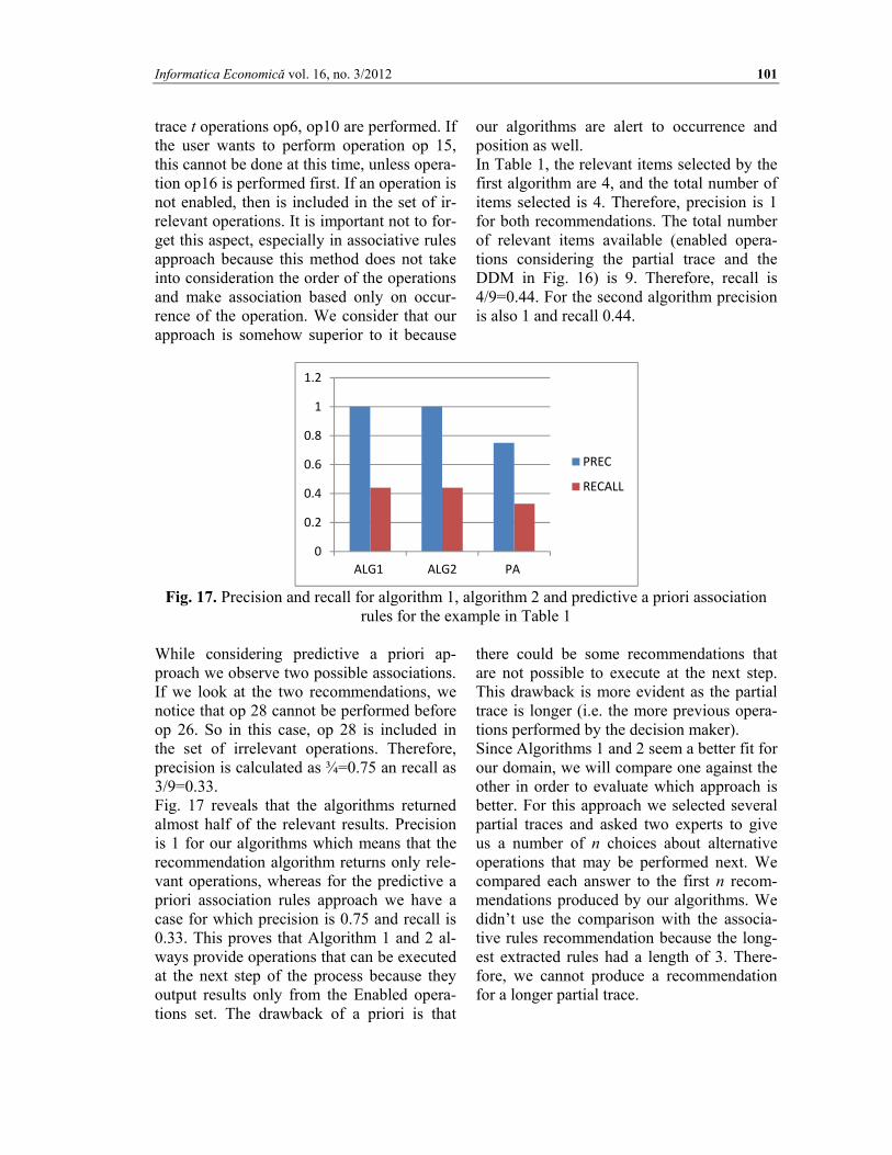
our algorithms are alert to occurrence and position as well. In Table 1, the relevant items selected by the first algorithm are 4, and the total number of items selected is 4. Therefore, precision is 1 for both recommendations. The total number of relevant items available (enabled opera-tions considering the partial trace and the DDM in Fig. 16) is 9. Therefore, recall is 4/9=0.44. For the second algorithm precision is also 1 and recall 0.44.

Fig. 17. Precision and recall for algorithm 1, algorithm 2 and predictive a priori association

rules for the example in Table 1 While considering predictive a priori ap-proach we observe two possible associations. If we look at the two recommendations, we notice that op 28 cannot be performed before op 26. So in this case, op 28 is included in the set of irrelevant operations. Therefore, precision is calculated as ¾=0.75 an recall as 3/9=0.33. Fig. 17 reveals that the algorithms returned almost half of the relevant results. Precision is 1 for our algorithms which means that the recommendation algorithm returns only rele-vant operations, whereas for the predictive a priori association rules approach we have a case for which precision is 0.75 and recall is 0.33. This proves that Algorithm 1 and 2 al-ways provide operations that can be executed at the next step of the process because they output results only from the Enabled opera-tions set. The drawback of a priori is that

there could be some recommendations that are not possible to execute at the next step. This drawback is more evident as the partial trace is longer (i.e. the more previous opera-tions performed by the decision maker). Since Algorithms 1 and 2 seem a better fit for our domain, we will compare one against the other in order to evaluate which approach is better. For this approach we selected several partial traces and asked two experts to give us a number of n choices about alternative operations that may be performed next. We compared each answer to the first n recom-mendations produced by our algorithms. We didn’t use the comparison with the associa-tive rules recommendation because the long-est extracted rules had a length of 3. There-fore, we cannot produce a recommendation for a longer partial trace.

0

0.2

0.4

0.6

0.8

1

1.2

ALG1 ALG2 PA

PREC

RECALL


Table 2. Recommendation comparison for algorithm 1, algorithm 2 and experts Partial trace Algorithm 1

Recommenda-tion

Algorithm 2 Recommendation

Expert 1 Rec

Expert 2 Rec

op1,op2,op6 op3,op14,op4 op14,op29,op5 op10,op16,op15 op3,op26,op10 op1,op6,op7 op2,op3,op14 op14,op24,op2 op24,op3,op27 op10,op26,opx1op1,op2,op3, op4

op6,op14,op29 op14,op29,op5 op27,op11,op22 op5,op6,opx2

op1,op2,op5, op18

op6,op14,op3 op14,op29,op20 op3,op4,op27 op3,opx3,opx4

op1,op2,op11, op8,op14

op6,op3,op29 op29,op5,op20 op22,-, - op5,op3,opx5

As it is observed in Table 2 we selected a number of 5 partial traces for which we expected recommendations from the algorithms developed and from accounting and decision process mining experts. We asked the experts to provide 3 alternative operations that might

be performed next. We consider that the process of evaluating algorithms recommendations is valid only if we compare the algorithms recommendations to the ones provided by experts. Therefore, we have calculated precision and recall metrics for every trace and showed the results in Fig. 18.

Fig. 18. Precision and recall for the five traces

We discovered that precision values for algorithm 1 was 0.67 in four out of five cases and one out of five for algorithm 2. This indicates that the recommendations algorithms return relevant operations in higher proportion than irrelevant operations. We have to discuss the 0 value for precision and recall for the recommendations provided by the second algorithm reffering to trace 106/107. This trace is an exception because none of the second algorithm recommendations were found in the set of relevant items. This set consists of all recommendations provided by experts. Therefore, for our study we considered the

union of operations recommend by expert 1 and expert 2 be the set of relevant items. The cardinal of this set is 18 operations. The explanation for this result is the small number of operations in the set of relevant items. We consider that asking more experts in the field for choices can lead to an increasing number of operations in the set of relevant items. Moreover, this leads to a higher probability that the recommendations provided by our algorithms are included in the set of relevant items and therefore precision gets higher. The highest value for recall is 0.33. This indicates that the algorithms returned some of the relevant

0

0.1

0.2

0.3

0.4

0.5

0.6

0.7

Precision alg1

Precision alg 2

Recall alg 1

Recall alg 2


result, but in none of the cases were recommended all relevant recommendations. We conclude that, the research presented in this paper strengthens the fact that providing recommendations is not an allways an easy task, although is performed by implemented software algorithms. 6 Conclusions The goal of our research is to improve deci-sion making by using a process model that explicitly shows the steps that need to be per-formed by the decision maker towards choos-ing one alternative. It is not our intention to recommend the better decision alternative. We want to make sure the decision makers made an informed decision by correctly and completely evaluating all alternatives. There-fore, the notion of recommendation used in this paper refers to the best next step (data aggregation operation) to be performed dur-ing the decision making process. To this end, we introduced two recommendation algo-rithms that rely on a model extracted before. The first algorithm simply recommends the most frequent operation(s) that may be exe-cuted at the next step. The second algorithm takes a more complex approach. It tries to guide the user towards a sub-objective of the decision process (e.g. evaluating some crite-rion). The paper explicitly shows how those two algorithms actually work and how they are implemented in our test application. To this end we provide both running examples and coding insights. The validation part of the paper introduces a comparison of the two algorithms with the association rules-based recommendations. We conclude that the classical approach is unfit to our domain because it produces rec-ommendations that cannot be executed. The second part of the validation section re-veals that the first algorithm produces better recommendations than the second. However, the conclusion is limited because of the dif-ference in decision making profiles of hu-mans. Still, the experiment we performed supports our claim that, if the essence of what a large number of decision makers is

extracted, the results are close enough to the performance of experts. The recommendation engine acts like an expert system by giving advice to the user while making the decision. Somehow, our decisions are influenced by others way of thinking. By taking such an as-pect into consideration, we trust more or less the global opinion of the crowd. As much as we discover their proficiency in opinion, the confidence gets a higher rate. These two al-gorithms are based on user’s interaction and the generality of opinions is granted by a large number of users. Acknowledgment: This work was supported by CNCS-UEFISCSU, project number PN II-RU 292/2010; contract no. 52/2010. References [1] R. Petruşel, P.L. Stanciu, Implementation

of a Recommendation Algorithm Based on the Decision Data Model, Proceedings of the 11th International Conference on Informatics in Economy (IE 2012), Edu-cation, Research & Business Technolo-gies, p.361-366.

[2] H.A. Simon.: The New Science of Man-agement Decision, Harper and Row, New York (1960)

[3] W.M.P. van der Aalst, Process Mining Discovery, Conformance and Enhance-ment of Business Processes, Springer, p. 352, (2011).

[4] B. Liu, Web Data Mining: Exploring Hy-perlinks, Contents, and Usage Data, 17 Data-Centric Systems and Applications, DOI 10.1007/978-3-642-19460-3_2, Springer-Verlag Berlin Heidelberg 2011

[5] R. Petruşel, I. Vanderfeesten, C.C. Dole-an, D. Mican, Making Decision Process Knowledge Explicit Using the Product Data Model. Lecture Notes in Business Information Processing, pp.172-184, Springer Verlag, 2011.

[6] R. Petruşel, P.L. Stanciu: Making Rec-ommendations for Decision Processes Based on Aggregated Decision Data Models, W. Abramowicz et al. (Eds.): BIS 2012, LNBIP 117, pp. 272–283,


2012, Springer-Verlag Berlin Heidelberg 2012

[7] S.J. Russell, P. Norvig, Artificial Intelli-gence: A Modern Approach, Prentice Hall, Upper Saddle River, 2003.

[8] L.H. Jonathan, A.J. Kostan, L.G. Ter-veen, J.T. Riedl, Evaluating Collaborative Filtering Recommender Systems, ACM

Transactions on Information Systems, Vol. 22, No.1, January 2004, Pages 5-53.

[9] R. Petruşel, Aggregating Individual Models of Decision-Making Processes, J. Ralyté et al. (Eds.): CAiSE 2012, LNCS 7328, pp. 47–63, Springer-Verlag Berlin Heidelberg 2012.

Paula Ligia STANCIU, Faculty of Economical Sciences and Business Ad-ministration, Babeş-Bolyai University, Cluj-Napoca, Romania, [email protected]. Paula Ligia Stanciu graduated the Faculty of Economics and Business Administration Babeş-Bolyai University, Cluj-Napoca in 2009. She holds from 2009 a bachelor degree in Economic Infor-matics, in the field of study Cybernetics, Statistics and Economic Informat-ics and a master degree in E-Business from 2011. She graduated the Faculty

of Mathematics and Computer Science at Babeş-Bolyai University, Cluj-Napoca in 2012 and holds from 2012 a bachelor degree in Mathematics. Her current research interests include De-cision Process Modeling, Process Mining, Decision Mining, Workflow Management.

Răzvan PETRUŞEL, Faculty of Economical Sciences and Business Ad-ministration, Babeş-Bolyai University, Cluj-Napoca, Romania, [email protected]. Răzvan Petruşel holds, from 2008, a Ph.D. in Cybernetics, Statistics and Business Informatics. He started in 2003 as a full-time Ph.D. student at the Business Information Systems Department, Economical Sciences and Business Administration Faculty, in Babeş-Bolyai University of Cluj-Napoca. In 2007 he became an assistant professor and

since 2009 he holds the current position as lecturer. His research is focused on Decision Min-ing, Modeling and Analysis; Software Design; Process Mining and Workflow Management.

implementing recommendation algorithms for decision making

Documents