implementing software defined radio -...
TRANSCRIPT

Eugene Grayver
Implementing SoftwareDefined Radio
123

Eugene GrayverWalnut Ave 2317Manhattan BeachCA 90266USA
ISBN 978-1-4419-9331-1 ISBN 978-1-4419-9332-8 (eBook)DOI 10.1007/978-1-4419-9332-8Springer New York Heidelberg Dordrecht London
Library of Congress Control Number: 2012939042
� Springer Science+Business Media New York 2013This work is subject to copyright. All rights are reserved by the Publisher, whether the whole or part ofthe material is concerned, specifically the rights of translation, reprinting, reuse of illustrations,recitation, broadcasting, reproduction on microfilms or in any other physical way, and transmission orinformation storage and retrieval, electronic adaptation, computer software, or by similar or dissimilarmethodology now known or hereafter developed. Exempted from this legal reservation are briefexcerpts in connection with reviews or scholarly analysis or material supplied specifically for thepurpose of being entered and executed on a computer system, for exclusive use by the purchaser of thework. Duplication of this publication or parts thereof is permitted only under the provisions ofthe Copyright Law of the Publisher’s location, in its current version, and permission for use must alwaysbe obtained from Springer. Permissions for use may be obtained through RightsLink at the CopyrightClearance Center. Violations are liable to prosecution under the respective Copyright Law.The use of general descriptive names, registered names, trademarks, service marks, etc. in thispublication does not imply, even in the absence of a specific statement, that such names are exemptfrom the relevant protective laws and regulations and therefore free for general use.While the advice and information in this book are believed to be true and accurate at the date ofpublication, neither the authors nor the editors nor the publisher can accept any legal responsibility forany errors or omissions that may be made. The publisher makes no warranty, express or implied, withrespect to the material contained herein.
Printed on acid-free paper
Springer is part of Springer Science+Business Media (www.springer.com)

To my parents, who have taught me how tobe happy, and that there’s more to life thanscience. And to my grandparents, who valuescience above all and have inspired andguided me in my career

Preface
A search for ‘Software Defined Radio’ on Amazon.com at the end of 2010 showsthat almost 50 books have been written on the subject. The earliest book waspublished in 2000 and a steady stream of new titles has been coming out since.So why do I think that yet another book is warranted?
SDR is now a mature field, but most books on the subject treat it as a newtechnology and approach SDR from a theoretical perspective. This book bringsSDR down to earth by taking a very practical approach. The target audience ispracticing engineers and graduate students using SDR as a tool rather than an endunto itself, as well as technical managers overseeing development of SDR. Ingeneral, SDR is a very practical field—there just isn’t very much theory that isunique to flexible radios versus single function radios.1 However, the devil is in thedetails… a designer of an SDR is faced with a myriad of choices and tradeoffs andmay not be aware of many of them. In this book I cover, at least superficially, mostof these choices. Entire books can be devoted to subjects treated in a few para-graphs2 below (e.g. wideband antennas). This book is written to be consulted at thestart of an SDR development project to help the designers pin down the hardwarearchitecture. Most of the architectures described below are based on actual radiosdeveloped by the author and his colleagues. Having built, debugged, and tested thedifferent radios; I will highlight some of the non-obvious pitfalls and hopefullysave the reader countless hours. One of my primary job responsibilities is oversightof SDR development by many government contractors. The lessons learned fromdozens of successful and less than successful projects are sprinkled throughout thisbook, mostly in the footnotes.
Not every section of this book addresses SDR specifically. The sections ondesign flow and hardware architectures are equally applicable to many otherdigital designs. This book is meant to be at least somewhat standalone since a
1 Cognitive radio, which is based on flexible radio technology, does have a significant theoreticalfoundation.2 The reader is encouraged to consult fundamental texts referenced throughout.
vii

practicing engineer may not have access to, or the time to read, a shelf full ofcommunications theory books. I will therefore guide the reader through a whirl-wind tour of wireless communications in Appendix A.3 The necessarily superficialoverview is not meant to replace a good book on communications [1,2] and thereader is assumed to be familiar with the subject.
The author does not endorse any products mentioned in the book.
3 The reader is encouraged to at least skim through it to become familiar with terminology andnomenclature used in this book.
viii Preface

Acknowledgments
Most of the ideas in this book come from the author’s experiences at two com-panies—a small startup and a large government lab. I am fortunate to be workingwith a truly nulli secundus team of engineers. Many of the tradeoffs described inthis text have been argued for hours during impromptu hallway meetings. Thenature of our work at a government lab requires every engineer to see the bigpicture and develop expertise in a wide range of fields. Everyone acknowledgedbelow can move effortlessly between algorithm, software, and hardware devel-opment and therefore appreciate the coupling between the disciplines. This bookwould not be possible without the core SDR team: David Kun, Eric McDonald,Ryan Speelman, Eudean Sun, and Alexander Utter. I greatly appreciate theinvaluable advice and heated discussions with Konstantin Tarasov, Esteban Valles,Raghavendra Prabhu, and Philip Dafesh. The seeds of this book were planted yearsago in discussions with my fellow graduate students and later colleagues, AhmedElTawil and Jean Francois Frigon.
I am grateful to my twin brother for distracting me and keeping me sane.Thanks are also due to my lovely and talented wife for editing this text and puttingup with all the lost vacation days.
ix

Contents
1 What is a Radio? . . . . . . . . . . . . . . . . . . . . . . . . . . . . . . . . . . . . 1
2 What Is a Software-Defined Radio?. . . . . . . . . . . . . . . . . . . . . . . 5
3 Why SDR? . . . . . . . . . . . . . . . . . . . . . . . . . . . . . . . . . . . . . . . . . 93.1 Adaptive Coding and Modulation . . . . . . . . . . . . . . . . . . . . . 10
3.1.1 ACM Implementation Considerations . . . . . . . . . . . . 163.2 Dynamic Bandwidth and Resource Allocation . . . . . . . . . . . . 173.3 Hierarchical Cellular Network . . . . . . . . . . . . . . . . . . . . . . . 193.4 Cognitive Radio . . . . . . . . . . . . . . . . . . . . . . . . . . . . . . . . . 203.5 Green Radio . . . . . . . . . . . . . . . . . . . . . . . . . . . . . . . . . . . 253.6 When Things go Really Wrong . . . . . . . . . . . . . . . . . . . . . . 26
3.6.1 Unexpected Channel Conditions . . . . . . . . . . . . . . . . 273.6.2 Hardware Failure . . . . . . . . . . . . . . . . . . . . . . . . . . 273.6.3 Unexpected Interference . . . . . . . . . . . . . . . . . . . . . 28
3.7 ACM Case Study . . . . . . . . . . . . . . . . . . . . . . . . . . . . . . . . 293.7.1 Radio and Link Emulation. . . . . . . . . . . . . . . . . . . . 303.7.2 Cross-Layer Error Mitigation . . . . . . . . . . . . . . . . . . 32
4 Disadvantages of SDR. . . . . . . . . . . . . . . . . . . . . . . . . . . . . . . . . 374.1 Cost and Power . . . . . . . . . . . . . . . . . . . . . . . . . . . . . . . . . 374.2 Complexity . . . . . . . . . . . . . . . . . . . . . . . . . . . . . . . . . . . . 384.3 Limited Scope . . . . . . . . . . . . . . . . . . . . . . . . . . . . . . . . . . 40
5 Signal Processing Devices . . . . . . . . . . . . . . . . . . . . . . . . . . . . . . 435.1 General Purpose Processors . . . . . . . . . . . . . . . . . . . . . . . . . 435.2 Digital Signal Processors . . . . . . . . . . . . . . . . . . . . . . . . . . . 445.3 Field Programmable Gate Arrays . . . . . . . . . . . . . . . . . . . . . 44
xi

5.4 Specialized Processing Units . . . . . . . . . . . . . . . . . . . . . . . . 475.4.1 Tilera Tile Processor. . . . . . . . . . . . . . . . . . . . . . . . 49
5.5 Application-Specific Integrated Circuits . . . . . . . . . . . . . . . . 515.6 Hybrid Solutions . . . . . . . . . . . . . . . . . . . . . . . . . . . . . . . . 515.7 Choosing a DSP Solution . . . . . . . . . . . . . . . . . . . . . . . . . . 52
6 Signal Processing Architectures. . . . . . . . . . . . . . . . . . . . . . . . . . 556.1 GPP-Based SDR. . . . . . . . . . . . . . . . . . . . . . . . . . . . . . . . . 55
6.1.1 Nonrealtime Radios . . . . . . . . . . . . . . . . . . . . . . . . 586.1.2 High-Throughput GPP-Based SDR . . . . . . . . . . . . . . 60
6.2 FPGA-Based SDR . . . . . . . . . . . . . . . . . . . . . . . . . . . . . . . 606.2.1 Separate Configurations. . . . . . . . . . . . . . . . . . . . . . 616.2.2 Multi-Waveform Configuration . . . . . . . . . . . . . . . . 616.2.3 Partial Reconfiguration . . . . . . . . . . . . . . . . . . . . . . 62
6.3 Host Interface . . . . . . . . . . . . . . . . . . . . . . . . . . . . . . . . . . 686.3.1 Memory-Mapped Interface to Hardware . . . . . . . . . . 696.3.2 Packet Interface . . . . . . . . . . . . . . . . . . . . . . . . . . . 73
6.4 Architecture for FPGA-Based SDR. . . . . . . . . . . . . . . . . . . . 736.4.1 Configuration . . . . . . . . . . . . . . . . . . . . . . . . . . . . . 736.4.2 Data Flow . . . . . . . . . . . . . . . . . . . . . . . . . . . . . . . 756.4.3 Advanced Bus Architectures . . . . . . . . . . . . . . . . . . 786.4.4 Parallelizing for Higher Throughput . . . . . . . . . . . . . 80
6.5 Hybrid and Multi-FPGA Architectures . . . . . . . . . . . . . . . . . 816.6 Hardware Acceleration . . . . . . . . . . . . . . . . . . . . . . . . . . . . 83
6.6.1 Software Considerations . . . . . . . . . . . . . . . . . . . . . 846.6.2 Multiple HA and Resource Sharing . . . . . . . . . . . . . 89
6.7 Multi-Channel SDR . . . . . . . . . . . . . . . . . . . . . . . . . . . . . . 92
7 SDR Standardization . . . . . . . . . . . . . . . . . . . . . . . . . . . . . . . . . 977.1 Software Communications Architecture and JTRS . . . . . . . . . 97
7.1.1 SCA Background . . . . . . . . . . . . . . . . . . . . . . . . . . 987.1.2 Controlling the Waveform in SCA . . . . . . . . . . . . . . 1037.1.3 SCA APIs . . . . . . . . . . . . . . . . . . . . . . . . . . . . . . . 104
7.2 STRS . . . . . . . . . . . . . . . . . . . . . . . . . . . . . . . . . . . . . . . . 1077.3 Physical Layer Description . . . . . . . . . . . . . . . . . . . . . . . . . 109
7.3.1 Use Cases . . . . . . . . . . . . . . . . . . . . . . . . . . . . . . . 1117.3.2 Development Approach . . . . . . . . . . . . . . . . . . . . . . 1117.3.3 A Configuration Fragment . . . . . . . . . . . . . . . . . . . . 1137.3.4 Configuration and Reporting XML . . . . . . . . . . . . . . 1157.3.5 Interpreters for Hardware-Centric Radios. . . . . . . . . . 1167.3.6 Interpreters for Software-Centric Radios . . . . . . . . . . 1167.3.7 Example . . . . . . . . . . . . . . . . . . . . . . . . . . . . . . . . 118
xii Contents
7.4 Data Formats . . . . . . . . . . . . . . . . . . . . . . . . . . . . . . . . . . . 1187.4.1 VITA Radio Transport (VITA 49, VRT) . . . . . . . . . . 1187.4.2 Digital RF (digRF) . . . . . . . . . . . . . . . . . . . . . . . . . 1257.4.3 SDDS . . . . . . . . . . . . . . . . . . . . . . . . . . . . . . . . . . 1257.4.4 Open Base Station Architecture Initiative . . . . . . . . . 1277.4.5 Common Public Radio Interface. . . . . . . . . . . . . . . . 128
8 Software-Centric SDR Platforms. . . . . . . . . . . . . . . . . . . . . . . . . 1318.1 GNURadio. . . . . . . . . . . . . . . . . . . . . . . . . . . . . . . . . . . . . 131
8.1.1 Signal Processing Blocks. . . . . . . . . . . . . . . . . . . . . 1328.1.2 Scheduler . . . . . . . . . . . . . . . . . . . . . . . . . . . . . . . 1358.1.3 Basic GR Development Flow. . . . . . . . . . . . . . . . . . 1368.1.4 Case Study: Low Cost Receiver
for Weather Satellites . . . . . . . . . . . . . . . . . . . . . . . 1378.2 Open-Source SCA Implementation: Embedded. . . . . . . . . . . . 1408.3 Other All-Software Radio Frameworks . . . . . . . . . . . . . . . . . 143
8.3.1 Microsoft Research Software Radio (Sora) . . . . . . . . 1438.4 Front End for Software Radio . . . . . . . . . . . . . . . . . . . . . . . 144
8.4.1 Sound-Card Front Ends . . . . . . . . . . . . . . . . . . . . . . 1458.4.2 Universal Software Radio Peripheral. . . . . . . . . . . . . 1458.4.3 SDR Front Ends for Navigation Applications. . . . . . . 1498.4.4 Network-Based Front Ends . . . . . . . . . . . . . . . . . . . 149
9 Radio Frequency Front End Architectures . . . . . . . . . . . . . . . . . 1519.1 Transmitter RF Architectures . . . . . . . . . . . . . . . . . . . . . . . . 151
9.1.1 Direct RF Synthesis . . . . . . . . . . . . . . . . . . . . . . . . 1529.1.2 Zero-IF Upconversion . . . . . . . . . . . . . . . . . . . . . . . 1549.1.3 Direct-IF Upconversion . . . . . . . . . . . . . . . . . . . . . . 1559.1.4 Super Heterodyne Upconversion. . . . . . . . . . . . . . . . 157
9.2 Receiver RF Front End Architectures . . . . . . . . . . . . . . . . . . 1579.2.1 Six-Port Microwave Networks . . . . . . . . . . . . . . . . . 158
10 State-of-the-Art SDR Components. . . . . . . . . . . . . . . . . . . . . . . . 15910.1 SDR Using Test Equipment . . . . . . . . . . . . . . . . . . . . . . . . . 159
10.1.1 Transmitter . . . . . . . . . . . . . . . . . . . . . . . . . . . . . . 16010.1.2 Receiver . . . . . . . . . . . . . . . . . . . . . . . . . . . . . . . . 16110.1.3 Practical Considerations . . . . . . . . . . . . . . . . . . . . . 163
10.2 SDR Using COTS Components . . . . . . . . . . . . . . . . . . . . . . 16510.2.1 Highly Integrated Solutions . . . . . . . . . . . . . . . . . . . 16510.2.2 Non-Integrated Solutions . . . . . . . . . . . . . . . . . . . . . 16610.2.3 Analog-to-Digital Converters (ADCs) . . . . . . . . . . . . 16710.2.4 Digital to Analog Converters (DACs) . . . . . . . . . . . . 171
Contents xiii

10.3 Exotic SDR Components . . . . . . . . . . . . . . . . . . . . . . . . . . . 17110.4 Tunable Filters . . . . . . . . . . . . . . . . . . . . . . . . . . . . . . . . . . 17310.5 Flexible Antennas. . . . . . . . . . . . . . . . . . . . . . . . . . . . . . . . 178
11 Development Tools and Flows . . . . . . . . . . . . . . . . . . . . . . . . . . . 18311.1 Requirements Capture . . . . . . . . . . . . . . . . . . . . . . . . . . . . . 18311.2 System Simulation . . . . . . . . . . . . . . . . . . . . . . . . . . . . . . . 18611.3 Firmware Development . . . . . . . . . . . . . . . . . . . . . . . . . . . . 188
11.3.1 Electronic System Level Design . . . . . . . . . . . . . . . . 18811.3.2 Block-Based System Design . . . . . . . . . . . . . . . . . . 19011.3.3 Final Implementation . . . . . . . . . . . . . . . . . . . . . . . 192
11.4 Software Development . . . . . . . . . . . . . . . . . . . . . . . . . . . . 19311.4.1 Real-Time Versus Non-Real-Time Software . . . . . . . 19311.4.2 Optimization . . . . . . . . . . . . . . . . . . . . . . . . . . . . . 19511.4.3 Automatic Code Generation . . . . . . . . . . . . . . . . . . . 196
12 Conclusion . . . . . . . . . . . . . . . . . . . . . . . . . . . . . . . . . . . . . . . . . 199
Appendix A: An Introduction to Communications Theory . . . . . . . . . 201
Appendix B: Recommended Test Equipment . . . . . . . . . . . . . . . . . . . 243
Appendix C: Sample XML Files for an SCA Radio . . . . . . . . . . . . . . 245
Bibliography . . . . . . . . . . . . . . . . . . . . . . . . . . . . . . . . . . . . . . . . . . . 253
Index . . . . . . . . . . . . . . . . . . . . . . . . . . . . . . . . . . . . . . . . . . . . . . . . 265
xiv Contents

Abbreviations
ACM Adaptive coding and modulationADC Analog to digital converterAMC See ACMASIC Application specific integrated circuit. Usually refers to a single-
function microchip, as opposed to a GPP or an FPGAAWGN Additive white Gaussian noiseCMI Coding and modulation information. A set of variables describing the
mode chosen by an ACM algorithmCORBA Common object request broker architecture. A standard that enables
software components written in multiple computer languages andrunning on multiple computers to work together. Used in SCA/JTRScompliant radios
COTS Commercial off-the-shelf. Refers to items that do not require in-housedevelopment
CR Cognitive radio. A radio that automatically adapts communicationsparameters based on observed environment
DAC Digital to analog converterdB Decibels. Usually defined as 10 log10ðA=BÞ if the units of A and B are
power, and 20 log10ðA=BÞ if the units of A and B are voltageDCM See ACMDDFS Direct digital frequency synthesizer. A digital circuit that generates a
sinusoid at a programmable frequencyDDS See DDFSDSP Digital signal processingDSSS Direct sequence spread spectrum. A modulation that uses a high-rate
pseudorandom sequence to increase the bandwidth of the signalEb/N0 Ratio of the signal energy used to transmit one bit to the noise level.
This metric is closely related to SNRENOB Effective number of bits. Used to characterize performance of an
ADC/DAC. Always less than the nominal number of bitsFEC Forward error correction
xv

FIFO First-in-first-out buffer. A fixed-length queueFIR Finite impulse response. Usually refers to a purely feed-forward filter
with a finite number of coefficientsFLOP Floating point operations per second. A metric used to computer signal
processing capabilities of different devices. Usually prefixed with ascale multiplier (e.g. GFLOPS for 109 FLOPS)
GbE Gigabit Ethernet. 10 GbE is 10 gigabit EthernetGPGPU General purpose GPU. A GPU with additional features to allow its use
for non-graphics applications such as scientific computingGPP General purpose processor. Major vendors include Intel, ARM, AMDGPU Graphics processing unit. A chip (usually in a PC) dedicated to
generating graphical output. A GPU is a key part of a video cardGUI Graphical user interfaceHPC High performance computing. Also known as scientific computing.
Many of the tools and techniques used in HPC are applicable to SDRdevelopment
Hz Unit of frequency, corresponding to one period per second (e.g. a 10Hz sine wave has 10 periods in 1 s)
I The in-phase (real) component of a complex valueIDL Inteface description language. Provides a way to describe a software
component’s interface in a language-neutral way. Used extensively inSCA-compliant radios
IF Intermediate frequency. Refers to either an RF carrier in a super-heterodyne front end, or to digitized samples at the ADC/DAC
IIR Infinite impulse response. Usually refers to a filter with feedbackIQ Inphase/quadrature (complex valued). Often refers to baseband signals
(vs. IF signals)LDPC Low density parity check code. A modern forward error correction
block code. Provides coding gain similar to that of a Turbo codeLSB Least significant bitMAC 1. Generic multiply and accumulate operation. See FLOP
2. Medium access control (network layer)MIMO Multiple input multiple output. A communications system employing
multiple antennas at the transmitter and/or receiverNVRAM Non-volatile memory. Memory that retains its data without power
(e.g. FLASH, EEPROM)OCP Open Core Protocol defines an interface for on-chip subsystem
communicationsOFDM Orthogonal frequency division multiplexing. A modulation scheme
that uses many tightly packed narrowband carriersOFDMA Orthogonal frequency division multiple access. Multi-user version of
the OFDM modulation. Multiple access is achieved in OFDMA byassigning subsets of subcarriers to individual users
xvi Abbreviations

OMG Object management group. A consortium focused on providingstandards for modeling software systems. Manages IDL and UMLstandards
OP Operation per second. See FLOPSPOSIX Portable Operating System Interface. A family of standards specified
by the IEEE for maintaining compatibility between operating systemsPR Partial reconfiguration. A technique to change the functionality of part
of the FPGA without disturbing operation of other parts of the sameFPGA
Q The quadrature (imaginary) component of a complex valueRF Radio frequencyRFFE RF front end – components of the radio from the antenna to the ADC/
DACRX, Rx Receive or receiverSCA Software communications architecture. Used in SCA/JTRS compliant
radiosSDR Software defined radioSDRAM Synchronous dynamic memory. Fast, inexpensive memory volatile
memorySF Spreading factor. Number of chips per symbol in a DSSS systemSIMD Single instruction multiple data. A programming paradigm and
corresponding hardware units that allow the same operation to beperformed on many values. SIMD instructions can be executed fasterbecause there is no overhead associated with getting a new instructionfor every data value
SISO Single input single output. A conventional communications systememploying one antenna at the transmitter and one at the receiver
SNDR Signal to noise and distortion ratio. Similar to SNR, but takes non-noise (e.g. spurs) distortions into account
SNMP Simple Network Management Protocol defines a standard method formanaging devices on IP networks. Commands can be sent to devicesto configure and query settings
SNR Signal to noise ratio. Usually expressed in dBsps Samples per second. Frequently used with a modifier (e.g. Gsps means
109 samples per second)SRAM Static random access memory. Memory content is lost when power is
removed. Data is accessed asynchronous. SRAM-based FPGAs usethis memory to store configuration
TX, Tx Transmit or transmitterUML Unified modeling language. A graphical language provides templates
to create visual models of object-oriented software systems. Used forboth requirements capture and automatic code generation
VLIW Very long instruction word. A microprocessor architecture thatexecutes operations in parallel based on a fixed schedule determinedwhen programs are compiled
Abbreviations xvii

VQI Video quality indicator. A quantitative metric related to the perceivedquality of a video stream. Range of 0 to 100
VRT VITA radio transport, VITA-49. A standard for exchanging data in adistributed radio system
VSWR Voltage standing wave ratio. Used as measure of efficiency forantennas. An ideal antenna has VSWR = 1:1, and larger numbersindicate imperfect signal transmission
w.r.t. With respect to
xviii Abbreviations

Chapter 1What is a Radio?
Before discussing software-defined radio, we need to define: what is a radio. For thepurposes of this book, a radio is any device used to exchange digital1 informationbetween point A and point B. This definition is somewhat broader than the standardconcept of a radio in which it includes both wired and wireless communications. Infact, most of the concepts that will be covered here are equally applicable to bothtypes of communications links. In most cases no distinction is made, since it isobvious that, for example, a discussion of antennas is only applicable to wirelesslinks. A top-level diagram of a generic radio2 is shown in Fig. 1.1.
In the case of a receiver, the signal flow is from left to right.
• Antenna. Electromagnetic waves impinge on the antenna and are converted intoan electrical signal. The antenna frequently determines the overall performanceof the radio and is one of the most difficult components to make both efficientand adaptable. The antenna can vary in complexity from a single piece of metal(e.g., a dipole) to a sophisticated array of multiple elements. In the past, anantenna was a passive component, and any adaptation was performed after thewave had been converted into an electrical signal. Some of the latest researchhas enabled the mechanical structure of the antenna itself to change in responseto channel conditions. Active and adaptive antennas will be discussed inSect. 10.5.
• Radio frequency (RF) front end. The electrical signal from the antenna is typ-ically conditioned by a RF front end (RFFE). The electrical signal is typicallyextremely weak3 and can be corrupted by even low levels of noise. The ambientnoise from the antenna must be filtered out and the signal amplified before it can
1 Analog radios are being rapidly phased out by their digital counterparts and will not be coveredin this book. Even the two major holdouts, AM and FM radios, are slowly being converted todigital.2 An entirely different kind of radio is described in [279]. All of the functionality is (incredibly)implemented in a single nanotube.3 A received signal power of -100 dBm (*2 lV) is expected by small wireless devices, while-160 dBm (*2 nV) received power is common for space communications.
E. Grayver, Implementing Software Defined Radio,DOI: 10.1007/978-1-4419-9332-8_1, � Springer Science+Business Media New York 2013
1

be processed further. The RF front end determines the signal-to-noise ratio(SNR) with which the rest of the radio has to work. A classical RF front endconsists of a filter, low noise amplifier, and a mixer to convert the signal fromradio frequency to a lower frequency. It is very challenging to design an RFfront end that is both efficient and flexible. These two elements are currently thelimiting factors in the development of truly universal radios. Classical andalternative RF front ends will be discussed in Chap. 9.
• Mixed signal converters. The amplified electrical signal at the output of the RFfront end may be digitized for further processing. Exponential improvement inthe speed and capacity of digital signal processing (DSP) has made DSP theobvious choice4 for the development of flexible radios. A mixed signal circuit(analog to digital converter) creates a digital representation of the receivedsignal. The digital representation necessarily loses some information due tofinite precision and sample rate. Allocation of resources (power, size, cost, etc.)between the RF front end and the mixed signal converters is a key tradeoff inSDR. The mixed signal components will be discussed in Sect. 10.2.
• Digital signal processing. DSP is applied to extract the information contained inthe digitized electrical signal into user data. The DSP section is (somewhatarbitrarily) defined as receiving the digitized samples from the mixed signalsubsection and outputting decoded data bits. The decoded data bits are typicallynot the final output required by the user and must still be translated into datapackets, voice, video, etc. A multitude of options are available to the radiodesigner for implementing the signal processing. A significant portion of this
Ant
enna
Rad
io F
requ
ency
Fron
t End
Mix
ed S
igna
l(A
nalo
g-D
igita
l)
Dig
ital S
igna
lPr
oces
sing
Net
wor
k an
dA
pplic
atio
ns
MIMOBeamformingNulling
Band selection (filter)Down-conversionLow noise amplifier
A/D converter AcquisitionDemodulationTrackingDecodingDecryption
AuthenticationRouting (TCP/IP)Data sink
Band selection (filter)Up-conversionPower amplifier
D/A converter ModulationEncodingEncryption
AuthenticationRouting (TCP/IP)Data source
MIMOBeamformingNulling
Fig. 1.1 Conceptual block diagram of a generic radio (transmit path on the top, receive at thebottom)
4 Papers presenting very creative and elegant approaches to analog implementation of traditionaldigital blocks are always being published (e.g., [274]), but are more exercises in design ratherthan practical solutions. Exceptions include niche areas such as ultra-low power and ultra-highrate radios.
2 1 What is a Radio?

book is devoted to describing various DSP options (Chap. 5) and architectures(Chap. 6). The exact functions implemented in the DSP section are determinedby the details of the waveform,5 but in general include:
– Signal acquisition. The transmitter, channel, and the receiver each introduceoffsets between the expected signal parameters and what is actually received.6
The receiver must first acquire the transmitted signal, i.e., determine thoseoffsets (see Sect. A.9.8).
– Demodulation. The signal must be demodulated to map the received signallevels to the transmitted symbols.7 Since the offsets acquired previously maychange with time, the demodulator may need to track the signal to continu-ously update the offsets.
– Decoding. Forward error correction algorithms used in most modern radiosadd overhead bits (parity) to the user data. Decoding uses these parity bits tocorrect bits that were corrupted by noise and interference.
– Decryption. Many civilian and most military radios rely on encryption toensure that only the intended recipient of the data can access it. Decryption isthe final step before usable data bits are available.
• Network and Applications. With the exception of a few very simple, point-to-point radios, most modern radios interface to a network or an application. In thepast, the network and applications were designed completely separately from theradio. SDR often requires tight coupling between the radio and the higher layers(see Table 2.1 ). This interaction will be discussed in Sect. 3.7 and mentionedthroughout the book.
5 Only receiver functionality is described here for brevity. Most functions have a correspondingequivalent in the transmitter.6 Typical offsets include differences in RF carrier frequency, transmission time, and signalamplitude.7 A simple demodulator maps a received value of +1 V to a data bit of ‘1’ and a received -1 V toa data bit of ‘0’. Modern demodulators are significantly more complex.
1 What is a Radio? 3

Chapter 2What Is a Software-Defined Radio?
Historically, radios have been designed to process a specific waveform.1 Single-function, application-specific radios that operate in a known, fixed environment areeasy to optimize for performance, size, and power consumption. At first glancemost radios appear to be single function—a first-generation cellular phone sendsyour voice, while a WiFi base station connects you to the Internet. Upon closerinspection, both of these devices are actually quite flexible and support differentwaveforms. Looking at all the radio devices in my house, only the garage dooropener and the car key fob seem to be truly fixed. With this introduction, clearly asoftware-defined radio’s main characteristic is its ability to support differentwaveforms.
The definition from wireless innovation forum (formerly SDR forum) states [3]:
A software-defined radio is a radio in which some or all of the physical layer functions aresoftware defined.
Let us examine each term individually:
• The term physical layer requires a bit of background. Seven different layers aredefined by the Open Systems Interconnection (OSI) model [4], shown inTable 2.1.
This model is a way of subdividing a communications system into smaller partscalled layers. A layer is a collection of conceptually similar functions thatprovide services to the layer above it and receives services from the layer belowit. The layer consisting of the first four blocks in Fig. 1.1 is known as thephysical layer.
• The broad implication of the term software defined is that different waveformscan be supported by modifying the software or firmware but not changing thehardware.
1 The term waveform refers to a signal with specific values for all the parameters (e.g., carrierfrequency, data rate, modulation, coding, etc).
E. Grayver, Implementing Software Defined Radio,DOI: 10.1007/978-1-4419-9332-8_2, � Springer Science+Business Media New York 2013
5

According to the strictest interpretation of the definition, most radios are notsoftware defined but rather software controlled. For example, a modern cellularphone may support both GSM (2G) and WCDMA (3G) standards. Since the user isnot required to flip a switch or plug in a separate module to access each network,the standard selection is controlled by software running on the phone. This definesthe phone as a software-controlled radio. A conceptual block diagram of such aradio is shown in Fig. 2.1. Software running on a microcontroller selects one of thesingle-function radios available to it.
A simple thought experiment shows that the definition of a true SDR is notquite as black and white as it appears. What if instead of selecting from a set of thecomplete radios, the software could select one of the building blocks shown inFig. 1.1? For example, the software would connect a particular demodulationblock to a decoder block. The next logical step calls for the software to configuredetails of the demodulator. For example, it could choose to demodulate QPSK or8PSK symbols. Taking this progression to an extreme, the software could defineinterconnect between building blocks as simple as registers, logic gates, andmultipliers, thereby realizing any signal processing algorithm. Somewhere in thisevolution, the software-controlled radio became a software-defined radio.
Micro -Processor
Radio forwaveform # 1
Radio for waveform # 2
Radio for waveform #N
cont
rol
Fig. 2.1 Basic software-controlled radio
Table 2.1 OSI seven-layer model
Data unit # Name Function
Host layers Data 7 Application Network process to application6 Presentation Data representation and encryption5 Session Interhost communication
Segment 4 Transport End-to-end connections and reliabilityMedia layers Packet 3 Network Path determination, logical addressing
Frame 2 Data Link Physical addressingBit 1 Physical Media, signal, and binary transmission
6 2 What Is a Software-Defined Radio?

The key, albeit subtle, difference is that a software-controlled radio is limited tofunctionality explicitly included by the designers, whereas a software-defined radiomay be reprogrammed for functionality that was never anticipated.
The ideal software-defined radio is shown in Fig. 2.2. The user data is mappedto the desired waveform in the microprocessor. The digital samples are thenconverted directly into an RF signal and sent to the antenna. The transmitted signalenters the receiver at the antenna, is sampled and digitized, and finally processed inreal time by a general purpose processor. Note that the ideal SDR in contrast withFig. 1.1, does not have an RFFE and a microprocessor has replaced the genericDSP block. The ideal SDR hardware should support any waveform at any carrierfrequency and any bandwidth.
So, what challenges must be overcome to achieve this elegant radioarchitecture?
• Most antennas are mechanical structures and are difficult to tune dynamically. Anideal SDR should not limit the carrier frequency or bandwidth of the waveform.The antenna should be able to capture electromagnetic waves from very lowfrequencies (e.g., \1 MHz) to very high frequencies (e.g. [60 GHz2).Section 10.5 detail the challenge of designing such an antenna. Such a widebandantenna, if available, places high demands on the RF front end (RFFE) and thedigitizer.
• Selection of the desired signal and rejection of interferers (channel selection) isa key feature of the RFFE. However, the antenna and filter(s) required toimplement the channel selection are usually electromechanical structures andare difficult to tune dynamically (see Sect. 10.4).
• Without an RF front end to select the band of interest, the entire band must bedigitized. Following Nyquist’s criterion, the signal must be sampled twice at themaximum frequency (e.g., 2 9 60 GHz). Capabilities of currently available A/Dconverters are discussed in Sect. 10.2.3, and are nowhere close to 120 GHz.
• The captured spectrum contains the signal of interest and a multitude of othersignals, as shown in Fig. 2.3. Interfering signals can be much stronger than thesignal of interest.3 A power difference of 120 dB is not unreasonable. The
A/DMicro-
ProcessorMicro-
ProcessorD/A
(a) (b)
Fig. 2.2 Ideal software-defined radio: (a) transmitter, (b) receiver
2 60 GHz is the highest frequency used for terrestrial commercial communications in 2011.3 Consider a practical example of a cell phone transmitting at +30 dBm while receiving a-60 dBm signal.
2 What Is a Software-Defined Radio? 7

digitizer must have sufficient dynamic range to process both the strong and theweak signals. An ideal digitizer provides about 6 dB of dynamic range per bit ofresolution. The digitizer would then have to provide well over 20 bits of reso-lution (e.g., 20 to resolve the interferer and more for the signal of interest).
• The digitizer must be very linear. Nonlinearity causes intermodulation betweenall the signals in the digitized band (see Fig. A-31 in Sect. A.9.6). Even a highorder intermodulation component of a strong signal can swamp a much weakersignal.
• In the extreme example discussed so far (a 24 bit digitizer operating at120 GHz) real-time digital signal processing has to be applied to a data streamat 120 9 109 9 24 & 250 GB/s. This is beyond the capabilities of modernprocessors and is likely to remain so in the foreseeable future.
Assuming all of these technical problems were solved,4 the same radio could beused to process any existing and expected future waveforms. However, it does notmean that radio is optimal or suitable for a given application. The ideal SDR maybe perfect for a research laboratory, where physical size and power consumptionare not an issue, but completely inappropriate for a handheld device. The next fewchapters will deal with the implementation tradeoffs for different market segments.
Some of the earliest software-defined radios were not wireless. The soft mod-ems used in the waning days of dial-up implemented sophisticated real-time signalprocessing entirely in the software.
0 Hz
120 dB
4GHz
Fs > 8GHz
Signal ofinterest
Large interferer
Fig. 2.3 Digitizing the signal of interest and adjacent bands
4 Note that the A/D converter with these specifications violates the Heisenberg uncertaintyprinciple and is therefore not realizable. The maximum A/D precision at 120 GSPS is limited to*14 bits [157] (see also footnote 6 of Chap. 10)
8 2 What Is a Software-Defined Radio?

Chapter 3Why SDR?
It takes time for a new technology to evolve from the lab to the field. Since SDR isrelatively new, it is not yet clear where it can be applied. Some of the mostsignificant advantages and applications are summarized below.
• Interoperability. An SDR can seamlessly communicate with multiple incom-patible radios or act as a bridge between them. Interoperability was a primaryreason for the US military’s interest in, and funding of, SDR for the past30 years. Different branches of the military and law enforcement use dozens ofincompatible radios, hindering communication during joint operations. A singlemulti-channel and multi-standard SDR can act as a translator for all the differentradios.
• Efficient use of resources under varying conditions. An SDR can adapt thewaveform to maximize a key metric. For example, a low-power waveform canbe selected if the radio is running low on battery. A high-throughput waveformcan be selected to quickly download a file. By choosing the appropriatewaveform for every scenario, the radios can provide a better user experience(e.g., last longer on a set of batteries).
• Opportunistic frequency reuse (cognitive radio.) An SDR can take advantage ofunderutilized spectrum. If the owner of the spectrum is not using it, an SDR can‘borrow’ the spectrum until the owner comes back. This technique has thepotential to dramatically increase the amount of available spectrum.
• Reduced obsolescence (future-proofing). An SDR can be upgraded in the field tosupport the latest communications standards. This capability is especiallyimportant to radios with long life cycles such as those in military and aerospaceapplications. For example, a new cellular standard can be rolled out by remotelyloading new software into an SDR base station, saving the cost of new hardwareand the installation labor.
• Lower cost. An SDR can be adapted for use in multiple markets and for multipleapplications. Economies of scale come into play to reduce the cost of each device.For example, the same radio can be sold to cell phone and automobile manu-facturers. Just as significantly, the cost of maintenance and training is reduced.
E. Grayver, Implementing Software Defined Radio,DOI: 10.1007/978-1-4419-9332-8_3, � Springer Science+Business Media New York 2013
9

• Research and development. An SDR can be used to implement many differentwaveforms for real-time performance analysis. Large trade-space studies can beconducted much faster (and often with higher fidelity) than through simulations.
The rest of this chapter covers a few of these applications in more detail.
3.1 Adaptive Coding and Modulation
The figure of merit for an SDR strongly depends on the application. Some radiosmust minimize overall physical size, others must offer the highest possiblereliability, while others must operate in a unique environment such as underwater.
For some, the goal is to minimize power consumption while maintaining therequired throughput. The power consumption constraint may be due to limitedenergy available in a battery-powered device, or heat dissipation for spaceapplications. The figure of merit for these radios is energy/bit [J/b].
Other radios are not power constrained (within reason, or within emitted powerlimits imposed by the FCC), but must transmit the most data in the availablespectrum. In that case, the radio always transmits at the highest supported power.The figure of merit for these radios is bandwidth efficiency—number of bitstransmitted per second for each Hz of bandwidth [bps/Hz]. Shannon’s law tells usthe absolute maximum throughput that can be achieved in a given bandwidth at agiven SNR. This limit is known as the capacity of the channel (see Sect. A.3).
C SNRð Þ ¼ B log2 1þ SNRð Þ
Shannon proved that there exists a waveform that achieves the capacity whilemaintaining an arbitrarily small BER. A fixed-function radio can conceivablyachieve capacity at one and only one value of SNR.1 In practice, a radio operatesover a wide range of SNRs. Mobile radios experience large changes in SNR overshort periods of time due to fading (see Sect. A.9.3). Fixed point-to-point radiosexperience changes in SNR over time due to weather. Even if environmentaleffects are neglected, multiple instances of the same radio are likely to be posi-tioned at different distances, incurring different propagation losses. Classical radiodesign of 20 years ago was very conservative. Radios were designed to operateunder the worst case conditions, and even then accepted some probability that thelink would be lost (i.e., the SNR would drop below a minimum threshold). In otherwords, the radios operated well below capacity most of the time and failed entirelyat other times.2
1 Given the assumptions of fixed bandwidth and fixed transmit power.2 Some radios changed the data rate to allow operation over a wide range of channel conditions.Reducing the data rate while maintaining transmit power increases SNR. However, capacity wasnot achieved since not all available spectrum was utilized.
10 3 Why SDR?

Adaptive coding and modulation3 (ACM) was introduced even before the SDRconcept (p. 19 in [5]). However, SDR made ACM practical. The basic idea followsstraight from Shannon’s law—select a combination of coding and modulation thatachieves the highest throughput given the current channel conditions whilemeeting the BER requirement [6]. Implementation of ACM has three basicrequirements:
1. Current channel conditions4 must be known with reasonable accuracy.2. Channel conditions must remain constant or change slowly relative to the
adaptation rate.3. The radio must support multiple waveforms that operate closer to capacity at
different SNRs.
The first requirement can be met taking either an open-loop or closed-loopapproach. In the open-loop approach, information about the channel comes fromoutside the radio. Examples include:
• Weather reports can be used to predict signal attenuation due to weather (e.g., ifrain is in the forecast, a more robust waveform is selected).
• Known relative position of the transmitter and receiver can be used to predictpath loss.
– GPS location information can be used to estimate the distance to a fixed basestation.
– Orbit parameters and current time can be used to estimate the distance to asatellite
A closed-loop (feedback) approach is preferred if the receiver can send infor-mation back to the transmitter (e.g., SNR measurements). This approach is morerobust and allows for much faster adaptation than open-loop methods. However, abidirectional link is required, and some throughput is lost on the return link toaccommodate the SNR updates. Almost all radios that support ACM are closed loop.
The second requirement is usually the greatest impediment to effective use ofACM. Consider a mobile radio using closed-loop feedback. The receiver estimatesits SNR and sends that estimate back to the transmitter which must process themessage and adjust its own transmission accordingly. This sequence takes time.During that time, the receiver may have moved to a different location and thechannel may have changed. The problem is exacerbated for satellite communi-cations, where the propagation delays can be of the order of � second.5
3 This technique falls in the category of Link Adaptation and is also known as dynamic codingand modulation (DCM), or adaptive modulation and coding (AMC).4 Channel conditions encompass a number of parameters (see Sect. A.9). The SNR is the onlyparameter used in the discussion below.5 A geostationary satellite orbits about 35,000 km above the earth. A signal traveling at thespeed of light takes 3.5 9 107 m/3 9 108 m/s = 0.12 s to reach it. Round trip delay is thenapproximately 0.25 s.
3.1 Adaptive Coding and Modulation 11

The channel for a mobile radio can be described by a combination of fast andslow fading. Fast fading is due to multipath (see Sect. A.9.3), while slow fading isdue to shadowing. ACM is not suitable for combating fast fading. The rate atwhich SNR updates are provided to the transmitter should be slow enough toaverage out the effect of fast fading, but fast enough to track slow fading. Theupdates themselves can be provided at different levels of fidelity: instantaneousSNR at the time of update, average SNR between two successive updates, or ahistogram showing the distribution of SNR between updates [7]. It is easy to showthat employing ACM with outdated channel estimates is worse than not employingit at all, i.e., using the same waveform at all times (see next page).
In the following discussion we derive and compare the theoretical throughputfor a link with and without ACM. For simplicity let us assume that the SDRsupports an infinite set of waveforms, allowing it to achieve capacity for everySNR.6 Consider a radio link where SNR varies from x to y (linear scale), withevery value having the same probability. Let the bandwidth allocated to the link be1 Hz. (Setting the bandwidth to 1 Hz allows us to use terms throughput andbandwidth efficiency interchangeably.)
Let us first compute the throughput for a fixed-function radio. This radio has topick one SNR value, s, at which to optimize the link. When the link SNR is belows, the BER is too high and no data are received. When the link SNR is above s, thetransmission is error-free. The average throughput of the link is then
P SNR [ sð Þ � C sð Þ þ P SNR\sð Þ � 0 ¼ y� s
y� x� log2 1þ sð Þ
The optimal s, which maximizes throughput, is easily found numerically for anyx, y. Numerical examples and graphs in this section are computed for x = 1 andy = 10 (0–10 dB). The capacity of the link varies between log2 1þ xð Þ (1 bps) andlog2 1þ yð Þ (3.5 bps). For our numerical example, shown in Fig. 3.1, optimals, s0 = 3.4, and the average throughput is 10�3:4
10�1 � log2 1þ 3:4ð Þ ¼ 1:6 bps.The average throughput is maximized but the system suffers from complete loss
of communications for s0 � xð Þ= y� xð Þ percent of the time (over 25 %), which isnot acceptable in many scenarios. For example, if the link is being used for ateleconference, a minimum throughput is required to maintain audio, while videocan be allowed to drop out. In these scenarios a single-waveform radio mustalways use the most robust waveform and will achieve throughput of only C(x)(1 bps).
Let us now compute the average throughput for an SDR that supports a widerange of capacity-approaching waveforms. Assuming the SNR is always perfectlyknown, the average throughput is simply
6 This assumption is not unreasonable since existing commercial standards such as DVB-S2define waveforms that operate close to capacity for a wide range of SNR (see Fig. 3.2).
12 3 Why SDR?

E C½ � ¼ 1y� x
Zx
y
C sð Þds ¼ 1þ yð Þ log2 1þ yð Þ � 1þ xð Þ log2 1þ xð Þy� x
� 1ln2
(equal to 2.6 bps for our numerical example).ACM actually degrades the link performance if SNR estimates are not available,
are out of date, or are inaccurate. Consider performance of ACM in a fast-fadingchannel when adaptation latency is longer than the channel coherence time. In thatcase, the waveform selection is uncorrelated to the channel conditions and can beconsidered to be random. Let the waveform selected by ACM be optimized forSNR ¼ a and let the actual SNR at the receiver equal b. No data can be sent whena [ b, which happens on average half the time. The other half of the time, linkthroughput is given by C(a). The average throughput is then 1
2 E C½ � (equal to 1.3 bpsfor our numerical example).
It is interesting to note that applying ACM with incorrect SNR updates resultsin slightly better throughput than always using the most robust waveform. Ofcourse, always using the most robust waveform has the major advantage ofguaranteeing no outages.
ACM is most effective if the expected7 link SNR falls within the ‘linear’ regionof the capacity curve (below 10 dB). The logarithmic curve flattens out at highSNR, meaning that capacity changes very little as SNR changes. If a radio operatesin the ‘flat’ region of the capacity curve, then a single waveform is sufficient.Advanced techniques such as MIMO (see Sect. A.6) can be leveraged to increase
1 2 3 4 5 6 7 8 9 100
0.5
1
1.5
2
2.5
3
3.5
SNR [linear]
Cap
acity
[bp
s]
Shannon capacitySingle-waveform capacitys0
Throughput at s 0
Fig. 3.1 Shannon and single-waveform capacity, s0 is the optimal s. X-axis is the target SNR
7 ACM can be invaluable for the unexpected decrease in SNR.
3.1 Adaptive Coding and Modulation 13
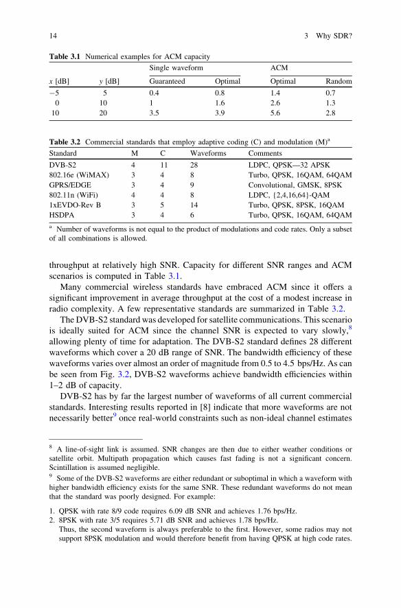
throughput at relatively high SNR. Capacity for different SNR ranges and ACMscenarios is computed in Table 3.1.
Many commercial wireless standards have embraced ACM since it offers asignificant improvement in average throughput at the cost of a modest increase inradio complexity. A few representative standards are summarized in Table 3.2.
The DVB-S2 standard was developed for satellite communications. This scenariois ideally suited for ACM since the channel SNR is expected to vary slowly,8
allowing plenty of time for adaptation. The DVB-S2 standard defines 28 differentwaveforms which cover a 20 dB range of SNR. The bandwidth efficiency of thesewaveforms varies over almost an order of magnitude from 0.5 to 4.5 bps/Hz. As canbe seen from Fig. 3.2, DVB-S2 waveforms achieve bandwidth efficiencies within1–2 dB of capacity.
DVB-S2 has by far the largest number of waveforms of all current commercialstandards. Interesting results reported in [8] indicate that more waveforms are notnecessarily better9 once real-world constraints such as non-ideal channel estimates
Table 3.1 Numerical examples for ACM capacity
Single waveform ACM
x [dB] y [dB] Guaranteed Optimal Optimal Random
-5 5 0.4 0.8 1.4 0.70 10 1 1.6 2.6 1.3
10 20 3.5 3.9 5.6 2.8
Table 3.2 Commercial standards that employ adaptive coding (C) and modulation (M)a
Standard M C Waveforms Comments
DVB-S2 4 11 28 LDPC, QPSK—32 APSK802.16e (WiMAX) 3 4 8 Turbo, QPSK, 16QAM, 64QAMGPRS/EDGE 3 4 9 Convolutional, GMSK, 8PSK802.11n (WiFi) 4 4 8 LDPC, {2,4,16,64}-QAM1xEVDO-Rev B 3 5 14 Turbo, QPSK, 8PSK, 16QAMHSDPA 3 4 6 Turbo, QPSK, 16QAM, 64QAM
a Number of waveforms is not equal to the product of modulations and code rates. Only a subsetof all combinations is allowed.
8 A line-of-sight link is assumed. SNR changes are then due to either weather conditions orsatellite orbit. Multipath propagation which causes fast fading is not a significant concern.Scintillation is assumed negligible.9 Some of the DVB-S2 waveforms are either redundant or suboptimal in which a waveform withhigher bandwidth efficiency exists for the same SNR. These redundant waveforms do not meanthat the standard was poorly designed. For example:
1. QPSK with rate 8/9 code requires 6.09 dB SNR and achieves 1.76 bps/Hz.2. 8PSK with rate 3/5 requires 5.71 dB SNR and achieves 1.78 bps/Hz.
Thus, the second waveform is always preferable to the first. However, some radios may notsupport 8PSK modulation and would therefore benefit from having QPSK at high code rates.
14 3 Why SDR?

and non-zero adaptation latency are taken into account. A link operating at the‘‘hairy edge’’ of a given waveform becomes susceptible to even small fluctuationsin SNR. Consider the waveforms in Table 3.3.
Only 0.6 dB separates these two waveforms, and the second one offers only7 % higher throughput. If the SNR estimate is incorrect or drops by 0.6 dB, ablock of data transmitted with waveform 2 will be lost. At least 1/0.07 & 15blocks have to be received correctly to compensate for the lost block and achievethe same average throughput as waveform 1. Larger spacing between SNR valuesrequired for different waveforms is acceptable, and in fact preferred, unless thechannel is static and the SNR estimates are very accurate.
-2 0 2 4 6 8 10 12 14 16 18
0.5
1
1.5
2
2.5
3
3.5
4
4.5
SNR [dB]
Ban
dwid
th E
ffici
ency
[bps
/Hz]
QPSK 1/4QPSK 1/3
QPSK 2/5
QPSK 1/2QPSK 3/5
QPSK 2/3QPSK 3/4
8PSK 2/3
8PSK 3/4
8PSK 5/68PSK 9/10
16APSK 3/4
16APSK 4/516APSK 5/6
16APSK 8/9
32APSK 3/4
32APSK 4/532APSK 5/6
32APSK 8/9
32APSK 9/10
QPSK 9/10
DVB-S2 waveforms
Shannon capacity
1 dB
2.5 dB
16APSK 2/3
Fig. 3.2 Spectral efficiency of DVB-S2
Table 3.3 DVB-S2 waveforms with almost identical throughput
# Modulation Code rate SNR [dB] Throughput [bps/Hz]
1 QPSK 3/4 3.9 1.52 QPSK 4/5 4.5 1.6
3.1 Adaptive Coding and Modulation 15

3.1.1 ACM Implementation Considerations
Although SDR is ideally suited for implementing ACM, a number of implemen-tation issues must be considered. Adaptation rate is an important implementationdriver. Fast ACM allows the code and modulation (CM) to change on a frame-by-frame basis. Slow ACM radio assumes that the CM changes infrequently and sometime is available for the radio to reconfigure. Most modern wireless standards relyon fast ACM. Fast ACM is an obvious choice for packet-based standard such asWiMAX. DVB-S2 is a streaming-based standard that also allows CM changes onevery frame. Fast ACM allows the radio to operate close to capacity even when thechannel changes relatively fast. Fast ACM is also used for point to multi-pointcommunications (i.e., when one radio is communicating simultaneously withmultiple radios) using TDMA. Each of the links may have a different SNR, and theradio has to change CM for each time slot.
For both fast and slow ACM, a mechanism is required for the receiver todetermine what CM was used by the transmitter for each set of received samples(frames or packets). Three most common mechanisms are:
1. Inserting the CM information (CMI) into each frame header. This is themechanism used by DVB-S2.
2. Passing the CMI on a side channel (e.g., control channel). This is the mecha-nism used by WiMAX.
3. Passing the CMI as part of the data payload in some frames.
The first two approaches are suitable for fast ACM, while the third is used forslow ACM. Providing CMI for every frame is inefficient if the channel is known tochange slowly. The overhead required to transmit CMI is then wasted most of thetime. CMI must be received correctly with very high probability since an error inCMI always leads to complete loss of the frame it described. For example, inDVB-S2 CMI is encoded using a rate 7/64 code (45 bits are used to send 5 bits ofCMI) and modulated with BPSK. This overhead is negligible10 for the long framesused by DVB-S2, but could be unacceptable for shorter frames.
An all-software radio can easily support fast ACM since all of the functionsrequired to implement each CM are always available. Supporting fast ACM on anFPGA-based SDR is more challenging. Consider three different FPGA reconfig-uration options described in Sect. 6.2. Fast ACM can be supported if the FPGAcontains all the functions required to implement each CM. If a different configu-ration has to be loaded to support a specific CM, the radio is not available duringthe reconfiguration time and fast ACM cannot be supported. Partial reconfigurationcan be used to support fast ACM if the FPGA has enough resources to simulta-neously support multiple (but not all) CMs.
10 Worst case overhead occurs for the shortest frames. For DVB-S2, the shortest frame (16200bit) transmitted using the highest modulation (32-APSK) requires a total of 3240 symbols. In thatcase the overhead is 45/3240 = 1%.
16 3 Why SDR?

3.2 Dynamic Bandwidth and Resource Allocation
The ACM technique described above can be extended to vary the signal band-width. Channel capacity grows monotonically with the available bandwidth.Therefore, most single-user point-to-point radios use all the bandwidth allocated tothem. However, if multiple users share the same spectrum, per-user bandwidthallocation becomes an important degree of freedom. Traditionally, frequencydivision multiple access (FDMA) approach was used to allocate the same amountof spectrum to each user. Modern radios allow each user to process different signalbandwidths at different times. There are three major techniques to achieve this:
1. A single-carrier radio can change its symbol rate, since occupied bandwidth islinearly related to the symbol rate. This approach was selected for the nextgeneration of military satellites (TSAT) [9].
2. A radio may be allowed to transmit on multiple channels. For example, GSMdefines each channel to be 150 kHz, but one radio can use multiple adjacentchannels.
3. Orthogonal frequency division multiple access (OFDMA) is the technique usedby many modern wireless standards to allocate subsets of OFDM (see Sect.A.4.7 and [10, 11]) subcarriers to different users. This is equivalent to (2) in thecontext of OFDM (i.e., subcarriers are orthogonal and separated by the symbolrate).
DBRA works well with ACM in a multi-user environment, where differentusers have uncorrelated SNR profiles. At any given time some users will experi-ence low SNR, while others will have high SNR.
Consider a system in which all users are accessing real-time streaming data(e.g., voice or video). Each user must maintain constant throughput to avoiddropouts. The overall system is constrained by the total allocated bandwidth andtotal transmit power. High SNR users can adapt CM to achieve high bandwidthefficiency and can maintain the required throughput at a lower symbol rate.Lowering the symbol rate frees up bandwidth that can be allocated to the low SNRusers as shown in Fig. 3.3. Alternatively, this goal could be achieved by allocatingmore power to the nominally low SNR user (thus increasing its SNR) and lesspower to the high SNR user.
The simple example below demonstrates the advantage of using DBRA andACM instead of just power control. A more general treatment of the same prob-lem, but in the context of OFDM, is presented in [12].
A radio is sending data to two users. The channel to user 2 has X times(10 log10 X dB) higher attenuation than the channel to user 1. Let the total powerbe P ¼ P1 þ P2. The total bandwidth is B ¼ B1 þ B2, which makes user 2’sbandwidth B2 ¼ B� B1. The first user’s capacity is:
C1 ¼ B1 log2 1þ P1
N0B1
� �
3.2 Dynamic Bandwidth and Resource Allocation 17

Expressing the second user’s capacity in terms of first user’s bandwidth, we get
C2 ¼ B� B1ð Þ log2 1þ P2=X
N0 B� B1ð Þ
� �
And, since both users require the same throughput,
C1 ¼ C2 ¼ C
We want to find the bandwidth allocation that minimizes total power, P. Solvingfor P1 and P2, we get
P1 B1ð Þ ¼ B1N0 2C
B1
� �� 1
!
P2 B1ð Þ ¼ B� B1ð Þ N0Xð Þ 2C
B�B1
� �� 1
!
Total power is then
PDBRA ¼ P1 B1ð Þ þ P2ðB1Þ
We can find B1 = Bopt that minimizes P numerically. Somewhat unexpectedly,Bopt is independent of N0.
If only ACM is available and the symbol rate (i.e., bandwidth) for both users is thesame, B1 = B2 = B/2, the second user has to be allocated X times more power toachieve the same capacity as the first user. Total power for the ACM-only case is then
PNO DBRA ¼ P1B
2
� �þ P2
B
2
� �¼ ð1þ XÞP1
B
2
� �
It is interesting to compare the power advantage, R, offered by DBRA
R ¼ PDBRA
PNO DBRA
Low SNR user :QPSK
Pow
er
Frequency
High SNR user :QPSK
Low SNR user :QPSK
Pow
er
Frequency
HighSNRuser :
16QAM
(a) (b)
Fig. 3.3 Applying DBRA to a two-user channel a no DBRA, b with DBRA
18 3 Why SDR?

Consider a numerical example, where B = 1 and X = 10 dB. A plot of R for arange of capacity values is shown in Fig. 3.4. As can be seen from this figure,DBRA offers only a modest improvement of about 1 dB, and only for highbandwidth efficiency. The improvement is more significant for a larger powerdifference among the users, X = 20 dB.
Another view of DBRA is offered in the numerical example below. For variety,let B = 1 MHz, X = 20 dB, and C = 1 Mbps. Solving for Bopt, we get the resultsin Table 3.4. For this scenario, R = 1.1 dB.
This somewhat disappointing result does not mean that DBRA is not a usefultechnique. For the TSAT program, DBRA was used to ensure that high-priorityusers can get high-throughput links even under very bad channel conditions (at thecost of lower or no throughput for other users).
3.3 Hierarchical Cellular Network
A mobile user has access to different wireless networks in different locations. Forexample, at home a user can access his wireless LAN; 4G cellular network isavailable outside his house; 2G network covers outside major metropolitan areas;and only satellite coverage is available in the wilderness. Each of these networks
0.5 1 1.5 2 2.5 3 3.5 4 4.5 50
0.5
1
1.5
2
2.5
3
3.5
4
4.5
PNO DBRA / PDBRA
Pow
er r
atio
[dB
]
Throughput [bps/Hz]
X = 10 dB
X = 20 dB
Fig. 3.4 Improvement offered by DBRA
3.2 Dynamic Bandwidth and Resource Allocation 19

uses a different waveform which is optimized for the target environment (e.g.,802.11 for LAN, LTE for 4G, GSM for 2G, Iridium for satellite) (Fig. 3.5).
The most ‘local’ network usually provides better service for those that coverwider areas. The user’s device consumes less power (extending battery life),typically gets higher throughput, and almost always incurs lower charges. The usercan carry four different devices to ensure optimal connectivity in all of theseenvironments. In that case, the connection on each device would be dropped as hetraveled outside its coverage area. Alternatively, the user can rely on the widestcoverage network (satellite), suffer poor battery life, and high cost, and still not beable to maintain a call inside a building. Dropped calls can be avoided by inte-grating all four radios into a single device and implementing handover betweenthem.11 Soft handover requires the ‘next’ radio to be ready before the ‘previous’radio is disconnected. This means that both radios must be active for some time.The ‘next’ radio must have enough time to acquire the signal. This approach isshown in Fig. 2.1.
An SDR combines all the separate radios into one, and almost surely simplifieshandover between networks. The internal state (e.g., absolute time, or channelestimate if the two networks share the same carrier frequency) is preserved duringhandover, reducing the amount of time required to lock onto the new signal.
3.4 Cognitive Radio
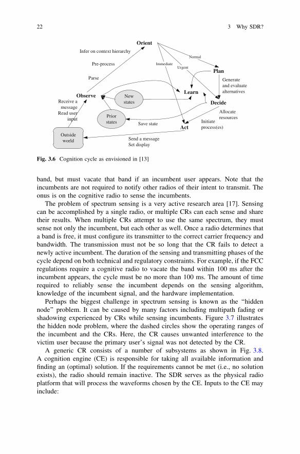
The concepts of software-defined radio and cognitive radio (CR) were both pro-posed by Joseph Mitola III [13]. In this ‘big picture’ paper, Mitola envisionedradios that are not only reconfigurable but are also aware of the context in whichthey are being operated. Such radios consider all observable parameters to selectthe optimal set of communications parameters. Theoretically, one such radio could‘‘see’’ a wall between the receiver and itself and choose to operate at a carrierfrequency that would be least attenuated by that wall, while taking into account allother radios around it. The cognition cycle responsible for processing all inputsand making appropriate decisions is depicted in Fig. 3.6. The radio responds toexternal stimuli by first orienting itself to the urgency of the events. Some events(e.g., battery level critical) must be responded to immediately, while others
Table 3.4 Optimal bandwidth allocation for a two-user DBRA scenario
User Bandwidth[kHz]
Power[relative N0]
SNR [dB] Efficiency [bps/Hz] Waveform
1 200 5.8 14.5 4.9 32-APSK, rate = 9/102 800 111 21.5 1.3 QPSK, rate = 2/3
11 Of course, the different networks have to support soft handover at the protocol layer.
20 3 Why SDR?

(e.g., motion detected) allow the radio some time to come up with an optimalsolution. For example, the ACM technique described previously uses only theinner (Observe, Orient, Act) loop. A key part of a true cognitive radio is ability tolearn (in the Learn state) what the outcome of a given decision will be. Forexample, it could automatically learn which CM is optimal for a given SNR. Thedecisions are then driven by all previously learned data and a set of predefinedconstraints which depend on the radio’s context (e.g., carrier frequency1.5–1.6 GHz can be used if the radio is in Europe, but 2.0–2.1 GHz if the radio isin the US). The combination of predefined and learned data allows a radio to workout-of-the-box and provide better performance over time.
We are still a long way from implementing such an intelligent radio, and it isnot at all clear whether there is a need for it. For now, the ambitions for CR havebeen scaled back to a ‘‘spectrum aware’’ radio [14]. Design of a spectrum-awareradio is motivated by the realization that spectrum is a precious shared resource.Most of the desirable spectrum (see Sect. A.2) is allocated to users (by the FCC inthe United States [15] and equivalent organizations around the world). Forexample, a local FM radio station is allocated a band at 98.3 MHz within a certaingeographic area. As new technologies such as cellular phones become available,they compete for spectrum resources with incumbent (also known as primary)users. The latest smartphones can process data rates of many Mbps to provideusers with streaming video. A significant amount of spectrum is required totransmit that much data. Bands allocated to cell phones were sized with only voicetraffic in mind and are heavily congested. Police, emergency medical, and otherpublic safety personnel also need more spectrum than their existing allocation,especially during a large-scale emergency [16].
Spectrum management agencies have long known that allocated spectrum isunderutilized. At any given time, only a small fraction of the allocated bands are inuse by the incumbents. In many areas, not all TV and radio stations are active.Some bands (e.g., those allocated for emergency satellite control) are used only afew minutes a day. A spectrum-aware CR is allowed to transmit in the allocated
WiFi LTEGSM Satellite
Fig. 3.5 Hierarchical network coverage
3.4 Cognitive Radio 21
band, but must vacate that band if an incumbent user appears. Note that theincumbents are not required to notify other radios of their intent to transmit. Theonus is on the cognitive radio to sense the incumbents.
The problem of spectrum sensing is a very active research area [17]. Sensingcan be accomplished by a single radio, or multiple CRs can each sense and sharetheir results. When multiple CRs attempt to use the same spectrum, they mustsense not only the incumbent, but each other as well. Once a radio determines thata band is free, it must configure its transmitter to the correct carrier frequency andbandwidth. The transmission must not be so long that the CR fails to detect anewly active incumbent. The duration of the sensing and transmitting phases of thecycle depend on both technical and regulatory constraints. For example, if the FCCregulations require a cognitive radio to vacate the band within 100 ms after theincumbent appears, the cycle must be no more than 100 ms. The amount of timerequired to reliably sense the incumbent depends on the sensing algorithm,knowledge of the incumbent signal, and the hardware implementation.
Perhaps the biggest challenge in spectrum sensing is known as the ‘‘hiddennode’’ problem. It can be caused by many factors including multipath fading orshadowing experienced by CRs while sensing incumbents. Figure 3.7 illustratesthe hidden node problem, where the dashed circles show the operating ranges ofthe incumbent and the CRs. Here, the CR causes unwanted interference to thevictim user because the primary user’s signal was not detected by the CR.
A generic CR consists of a number of subsystems as shown in Fig. 3.8.A cognition engine (CE) is responsible for taking all available information andfinding an (optimal) solution. If the requirements cannot be met (i.e., no solutionexists), the radio should remain inactive. The SDR serves as the physical radioplatform that will process the waveforms chosen by the CE. Inputs to the CE mayinclude:
Outsideworld
Priorstates
Newstates
ObserveReceive a
messageRead user
input
Orient
Parse
Pre-process
Infer on context hierarchy
Plan
Normal
Decide
Urgent
Act
Immediate
Allocate resources
Initiate process(es)
Send a messageSet display
Learn
Save state
Generateand evaluatealternatives
Fig. 3.6 Cognition cycle as envisioned in [13]
22 3 Why SDR?

• FCC regulations (e.g., vacate in 100 ms, maximum transmit power is 1 W, etc.)• User bandwidth requirement (e.g., need 1 Mbps to stream video).• Remaining battery level and how long the battery should last. If the transmission
given available bandwidth would require too much power, the radio should nottransmit.
• Spectrum-sensing output that includes a list of bands open for transmission.• Geographical position. Position could determine the applicable regulations (e.g.,
different in Europe and USA).• Radio environment could be derived from the geographical position. The
optimal modulation in an urban setting is different from that in a rural setting.
PrimaryUser
Cogntiveradios
Incumbent’s signal does not reach the cognitive radio
VictimUser
Fig. 3.7 The ‘hidden node’ problem for spectrum sensing
Cognitive
engine
Spectrum
sensing
SDR
SplitterRF
RF
Spectrum
occupancy
Configuration
User Data
Rad
io c
onte
xt:
Reg
ulat
ions
, use
r
requ
irem
ents
, etc
.
Fig. 3.8 Block diagram of a cognitive radio
3.4 Cognitive Radio 23

CE can be as simple as a hard-coded flowchart or as complex as a self-learninggenetic algorithm [18] or other artificial intelligence algorithms [19]. Each of thethree major blocks in the figure require specialized expertise to develop, and asystem integrator may choose to procure each block from a different vendor.A standard method for exchanging SDR configuration and spectrum occupancyresults would facilitate subsystem compatibility among different vendors. No suchstandard has yet been accepted by the SDR community, but one proposal is dis-cussed in Sect. 7.3.
As spectrum becomes more crowded, simply moving to a different frequencybecomes too restrictive. The latest work in CR considers simultaneous use of thesame band by multiple users. A technique known as multi-user detection (MUD12)can be applied to separate multiple overlapping signals [20]. The separation is onlyfeasible under certain conditions (e.g., signals from different users should besubstantially different to allow projection of each signal onto independent basis).An advanced CE determines whether a particular band is suitable for MUD andensures that all radios using the band can implement MUD or tolerate the addi-tional interference. Consider a scenario with a high-power one-way point-to-pointmicrowave link coexisting with low-power walkie-talkies (WT). Interference fromthe walkie-talkies to the microwave link is negligible. However, the microwavelink easily overpowers the walkie-talkies, as shown in Figure 3.9. The WTwaveform is very different from the microwave waveform. Further, the microwavewaveform is received by the WT with high power and high SNR. The WT can thenapply MUD to suppress the interfering microwave signal. The amount of sup-pression depends on the MUD algorithm, channel conditions, etc. These algo-rithms are computationally intensive and increase the power consumption of theDSP subsystem in WT. However, the reduction in WT transmit power madepossible by the interference mitigation often more than makes up for the powercost of the mitigation [21].
mic
row
ave m
icrowave
WT WT
Fig. 3.9 Application ofMUD to spectrum sharing
12 MUD can be extremely computationally expensive and has not been implemented in handhelddevices yet. However, it is only a matter of time….
24 3 Why SDR?

3.5 Green Radio
Radio engineers usually focus on optimizing a single communications link. Forexample, power consumption at a user terminal is optimized to increase batterylife. A new concept called green radio addresses the power consumption of theentire communications infrastructure. For the case of cellular telephony thatincludes power used by all the base stations, handsets, and network equipment.The network operators benefit from reduced power costs and positive publicity.
The radio interface accounts for about 70 % of the total power consumption andtherefore offers the largest potential for power savings. SDR provides the controlsto adapt the radio interface to minimize total power. A cognitive radio approachdescribed above can be applied to tune the controls [22]. The fundamentaltradeoffs enabled by SDR are described in [23] and shown in Figure 3.10. Themetrics identified in that paper are:
1. Deployment efficiency (DE) is a measure of aggregate network throughput perunit of deployment cost. The deployment cost consists of both the hardware(e.g., base station equipment, site installation, backhaul) and operationalexpenses (e.g., power costs, maintenance). Many closely spaced base stationsallow each to transmit at a lower power level. Received power decreases with(at least) the square of the distance and distance decreases linearly with numberof base stations. Thus, total power can be reduced by increasing the number ofbase stations, although the deployment cost increases.
2. Spectrum efficiency (SE) is a well-understood metric (see Sect. A.2). Energyefficiency (EE) is related to SE using Shannon’s capacity equation,EEð Þ ¼ SE
2SE�1ð ÞN0. This is a monotonically decreasing function. It appears that
the most robust waveforms (lowest SE) result in the highest EE. However, ifone considers the static power consumption of the transceiver electronics, theEE at very low SE actually decreases. It is easy to see that if one waveformtakes 1 min and another takes 1 s to transmit the same amount of data, the radiousing the first waveform must remain powered on for much longer. Thus, thereexists an optimum value of SE that maximizes EE.
3. Bandwidth (BW) and power (P) are two key constraints in a wireless system.
Using Shannon’s capacity equation, we can show that P ¼ BW � N02R
BW�1,which is a monotonically decreasing function. Thus, it is always beneficial touse all available bandwidth to reduce required power. For example, if a basestation is servicing just a few users, each user can be allocated more bandwidth[21]. The spectrum-aware radio approach described in the previous section canbe used to increase the amount of available bandwidth (also see [24]). TheDBRA approach described in Sect. 3.2 can then be applied to allocate band-width to users. Practically, this tradeoff is somewhat more complicated becausein practical systems power consumption increases when processing a largerbandwidth (i.e., a 1 Gsps ADC consumes much more power than a 1 MspsADC).
3.5 Green Radio 25

4. Delay (DL) is the last metric that is considered in optimization of energyefficiency. In the simplest case, delay can be related to throughput, which is inturn related to spectrum efficiency. Tolerating larger delays (slower transmis-sion) allows reduction in power. The effect is even more significant if weconsider operation in a fading channel. When a user is experiencing a fade,it requires more power to deliver data. If larger delays can be tolerated, thesystem can schedule transmissions to users with good channel conditions first.This approach, closely related to opportunistic beamforming [25], can signifi-cantly increase capacity and reduce power at the same time.
These tradeoffs are enabled by the degrees of freedom provided by a SDR. Themore degrees of freedom, (also known as knobs in CR literature), the closer thesystem can achieve optimal power consumption [26]. The basis for power con-sumption optimization at the physical layer is adaptive coding and modulation (seeSect. 3.1). The work in [26] delves deeper into the details of a waveform to studysecond-order parameters such as pilot symbols and number of antennas.
3.6 When Things go Really Wrong
True SDR (as opposed to software-controlled radio) really excels when unex-pected problems occur and the radio cannot be replaced or repaired. The bestexamples come from radios used in space, where the cost of failure is very highand no options for hardware repair exist.
Deployment efficiency
Bandwidthconsumption
Powerconsumption
Energyefficiency
Spectrumefficiency
Delayperformance
Energyefficiency
Powerconsumption
Capital/Operational expenditure Energy Efficiency Spectrum efficiency
Bandwidth Power Consumption Latency/QoS
Netw
ork performance
Net
wor
k C
ost
Fig. 3.10 Fundamental tradeoffs for green radio [23] (shaded blocks indicate negative effect ofimproving the white blocks)
26 3 Why SDR?

3.6.1 Unexpected Channel Conditions
The Cassini-Huygens mission was launched in 1997 to study Saturn and its moons.The Huygens probe was designed to separate from the main spacecraft and land onSaturn’s moon, Titan, 8 years after the launch. Huygens would transmit data toCassini, which in turn would retransmit it to the Earth. Long after launch, engi-neers discovered that the communication equipment on Cassini had a potentiallyfatal design flaw, which would have caused the loss of all data transmitted byHuygens.13 The radio on Cassini could not correctly compensate for the highDoppler shift experienced by Huygens during the rapid descent to the surface [27,28]. A small change to the symbol tracking algorithm in the Cassini radio couldhave fixed the problem, but the radio was not an SDR and could not be changed.Luckily, a solution was found by changing the flight trajectory of Cassini to reduceDoppler shift and all of the science data was returned. As noted in [28],‘‘Spacecraft systems need to have an appropriate level of reconfigurability inflight. This anomaly would have been easy to solve if there has been even a modestamount of reconfigurability in the [Cassini radio]’’. An SDR would have met thismodest requirement and could have allowed even more science data return byusing ACM during the descent.
3.6.2 Hardware Failure
Most software-controlled radios support a set of waveforms from a single family(e.g., linear modulations such as BPSK—16QAM or nonlinear modulations suchas GMSK, but not both). Very few scenarios require a radio to switch to a differentwaveform family. One illustrative example that did require changing waveformfamily involves a transmitter with a faulty carrier synthesizer. An ideal synthesizergenerates a pure sinusoid at the desired frequency, or equivalently the phase of theoutput is perfectly linear. A component failure in a synthesizer caused the outputphase to vary randomly at a very high rate. The phase tracking loop in the receivercould not keep up with the rapid changes, making demodulation impossible.Unlike the previous example (Cassini), changing the loop parameters or algorithmwould not be sufficient. Analysis showed that coherent demodulation wasimpossible without significantly increasing transmit power (which was not anoption). A waveform that can be demodulated noncoherently (see Sect. A.4.5)does not require a phase tracking loop and could solve the problem. A waveformsuch as differential BPSK (DBPSK) requires almost no additional DSP resourcescompared to BPSK and is easy to implement on the existing hardware. However,
13 Doppler shift results in both a frequency shift (compensated by Cassini radio) and symbolrate shift (not compensated). The symbol rate shift is negligible for small Doppler shifts and wasoverlooked by the engineers.
3.6 When Things go Really Wrong 27

even DBPSK suffered significant degradation is due to the rapid phase variations.FSK modulation can also be detected noncoherently and was found to be a bettersolution to the problem.
3.6.3 Unexpected Interference
Once a radio is out in the field, it can experience intentional or unintentionalinterference (also see A.9.5). A rich set of interference mitigation techniques isavailable. However, each technique is only applicable to a specific type of inter-ference. SDR provides radio engineers with powerful options for interferencemitigation. Consider a fielded military radio that experiences a previouslyunknown interferer (a jammer). The radio can characterize the jammer waveformor just capture a sequence of samples when the jammer is present. The informationis then passed to an analyst who can select the appropriate existing technique ordevelop a new one. The radio is then updated with software to mitigate thejammer. An autonomous jammer analyzer and mitigation technique selectionapproach, called cognitive antijam, is described in [29, 30]. The analyzer candistinguish between wideband burst and narrowband continuous jammers, asshown in Figure 3.11.
Jammer
analyzer
FFT-based
frequency
excision
Time-domain
blanking
Demodulator
Jammer parameters (frequency,
pulse times, etc.)
Select mitigation technique
Fig. 3.11 Cognitive antijam technique implemented in an SDR
28 3 Why SDR?

3.7 ACM Case Study
The physical layer techniques discussed above are only a part of a complete SDR.This section describes a case study aimed at evaluating the effectiveness of acombination of techniques in a complete system [31]. Three mitigation techniqueswere considered singly and together:
1. Adaptive coding and modulation (ACM) at the physical layer.2. Automatic repeat request (ARQ) at the network layer.3. Automatic codec adaptation (ACA) at the application layer.
The system in question is a next-generation military satellite used to providereal-time video feeds to commanders in the field. As discussed in Sect. A.9, mostwireless links must contend with channel fades and limited bandwidth. Satellitelinks have some unique properties (e.g., large propagation delays) that distinguishthem from terrestrial links.
A variety of techniques (e.g., FEC, channel interleaving, and ARQ) have beenproposed to mitigate satellite channel impairments, but it is not clear what effectthese mechanisms will have on upper layer protocols and end-user applications. Itis crucial to evaluate the cross-layer performance of these mitigation techniquesbefore they are deployed. A test bed consisting of a software-defined radio, a real-time wireless channel emulator (CH), and a network-layer emulator (SALEM) wasdeveloped to study end-to-end system performance. The SALEM also implementsnetwork-layer mitigation techniques such as ARQ. Figure 3.12 shows the archi-tecture of the integrated test bed for emulating future military communicationscenarios. The test bed and results are described in detail below.
Commercial test equipment that generates and analyzes packets (Agilent N2X[32]) was used to quantify the performance of cross-layer mitigation techniques.The techniques were compared based on standard network-layer metrics such aspacket loss ratio (PLR), latency, and throughput. Real-time performance ofcombinations of multiple mitigation schemes was observed with a streaming videoapplication.
Videoserver
SALEM2
SDRSALEM
1Videoclient
SDR Controller
SALEMController
Delay
Terminal 0 Terminal 1
SDRCH
Control plane
PHY
Fig. 3.12 Architecture of integrated test bed
3.7 ACM Case Study 29

3.7.1 Radio and Link Emulation
The physical layer emulator (PHY) consists of SDR and CH as shown in Fig. 3.13.It provides on-the-fly configurability to facilitate performance assessment undervarious communication scenarios. Four SDR transceivers are used to model a fullduplex link between two users over a fully processed satellite payload. User SDRsprovide a standard Ethernet interface. Each of the four links can use a differentwaveform. A wide range of waveforms (BPSK—64QAM) and data rates (1 kbps—40 Mbps) is supported. Additionally, forward error correction (e.g., Reed-Solo-mon, Viterbi, Turbo, LDPC, etc.), interleaving, and encryption are all supported[33]. The SDR transceiver is configured using an XML description of a waveform(described in Sect. 7.3). Waveforms can be reconfigured in a few milliseconds [33].
The channel emulator applies realistic impairments to the transmitted wave-form in real time. Both flat and frequency-selective (multipath) fading models aresupported. The channel emulator is implemented using a combination of softwareand hardware: channel coefficients are computed in software and applied to thewaveform in hardware (Fig. 3.14). The software can generate a range of channelscenarios such as line-of-sight, urban environment, and nuclear scintillation, andalso allows models to be imported via precomputed data files.
SALEM provides link-layer capabilities, such as link-layer error mitigation(ARQ), adaptive modulation and coding (ACM), application codec control (ACC),and packet segmentation/reassembly [34]. Figure 3.15 depicts the architecture ofSALEM integrated with PHY. In the integrated test bed, a delay node is insertedbetween SALEM2 and PHY to emulate the propagation delay incurred at thesatellite up and down links (0.25 s).
ARQ is a link-layer error mitigation technique based upon packet retransmis-sion. SALEM1 transmits an acknowledgment (ACK) frame for every packet itreceives from SALEM2.14 If SALEM2 does not receive an ACK frame for a
SDRTX
Channelemulator
SDRRX
SDRRX
Channelemulator
SDRTX
SDRTX
Channelemulator
SDRRX
SDRRX
Channelemulator
SDRTX
User 1
User 2
Sate
llite
Eth
Eth
switc
hsw
itch
Fig. 3.13 Physical layer emulation for the test bed
14 For clarity, only the link from user 1 to user 2 is described.
30 3 Why SDR?

predetermined interval, it retransmits the unacknowledged frame. Retransmissionis attempted up to a predetermined number of times.
SDR RX constantly monitors the SNR and periodically reports it to the ACMcontroller in SALEM1. SALEM1 then creates and sends a channel report (CR) toSALEM2. SALEM2 searches a database to find the optimal waveform supportedfor the SNR. If the optimal waveform is different from the current one, SDR TX isreconfigured. If a change in CM results in a change in the available bandwidth,SALEM2 sends a message to the video server to change the codec to match thevideo data rate to available bandwidth.
An open-source media player (VLC) was used for video encoding and play-back. A metric called the video quality indicator (VQI) was implemented in VLCto assess the quality of a video stream. A codec control interface was alsoimplemented in VLC to dynamically change the video compression per controlmessages from SALEM. Message exchange for ACM with video compressionadaptation is shown in Fig. 3.16.
LL
Fra
me
SAL
EM
1
SALEM 2
Segment-ation
ARQ-Tx
Re-Assembly
ARQ-Rx
IP P
acke
t
IP P
acke
t
ACM
ACC
ACK ReceiveLinkBandwidth
LL
Fra
me
SNRCR
PHY
Config
Fig. 3.15 SALEM block diagram
Cha
nnel
mod
el
Delay, scale, rotateDelay, scale, rotate
Delay, scale, rotate
From SDR
To SDR
Fig. 3.14 Channel emulator
3.7 ACM Case Study 31

3.7.2 Cross-Layer Error Mitigation
Cross-layer error mitigation tests were performed in two configurations: one withAgilent N2XTM and the other with a real-time streaming video application. Thefollowing subsections will describe in detail the test scenarios, including thechannel model, various physical-, link-, and application-layer parameters, andcorresponding results.
3.7.2.1 Performance Evaluation with a Traffic Analyzer
In this test, N2X is both the packet source and sink for the testbed, enablingautomated measurement of PLR, latency, and throughput (RxRate) (Fig. 3.17).Two types of fading channel were modeled, short fades and long fades, as listed inTable 3.5. In each model, the channel SNR follows a saw-tooth trajectory (linearin dB) between the minimum and maximum values over some duration. FEC wasdisabled for this test and modulation was allowed to vary between BPSK and16QAM when ACM was enabled and was fixed to 16QAM when ACM wasdisabled.
VideoServer
SALEM1
SDRTX
SDRRX
SALEM2
VideoClient
SNRestimate
SNR estimate
over uplink channelSet new
CMSet
compression Set newCM
Auto detect compression
Fig. 3.16 Message passing for ACM and video compression adaptation (time flows down)
SALEM2 PHY SALEM1
PHYControl & Monitor
SALEMControl & Monitor
DELAY
Agilent N2X
control plane
Fig. 3.17 Test bed with N2X
32 3 Why SDR?

Table 3.6 presents the test results with N2X, with a nominal transmit rate of1 Mbps. The ARQ retransmission interval was set to 550 ms, and the maximumretransmission count was 7.
In case 1.1, about 14 % of packets did not survive the fading channel while theSNR was low, which resulted in a lower Rx Rate. Average and maximum latenciesinclude both propagation and processing delays.
In case 1.2, the modulation automatically adapted to the current SNR, whichsignificantly reduced the packet losses. In case 1.3, ACM was disabled while ARQwas enabled. Despite retransmissions by ARQ, about 7 % of packets were lost.This demonstrates that during long fades, even 7 retransmissions were not enoughto save 7 % of packets. The average latency of 951 ms indicates each packet isretransmitted about 1.3 times on average.15 The maximum latency reflects themaximum number of retransmissions plus processing time and queuing delays.Compared to case 1.1, ARQ reduced the PLR by about 50 % at the cost ofincreased latency. In case 1.4, both ACM and ARQ were enabled. Most of thepackets made it through the fading channel, and packets dropped during the modechange were recovered by ARQ, which resulted in zero PLR. The increases in theaverage and maximum latencies compared to those from cases 1.1 and 1.2 weredue to retransmission of lost packets during the mode change.
In cases 2.1 through 2.4, the channel fluctuated much faster than in the previouscases. Case 2.1 lost about 11 % of packets, which is comparable to case 1.1. Incase 2.2, about 9 % of packets were lost despite ACM. Case 2.2 corresponds to the‘random SNR’ scenario discussed on page 13.
Table 3.5 Fading channel models
Model Max SNR (dB) Min SNR (dB) Duration (s)
Short fade 35 17 5Long fade 35 17 30
Table 3.6 Test results with N2X
Case ID Channelmodel
ACM ARQ PLR (%) RxRate(Mbps)
Avg. Lat. (ms) Max. Lat.(ms)
1.1 Long Off Off 14.07 0.83 252 2531.2 Long On Off 0 0.99 253 2551.3 Long Off On 7.05 0.91 951 55681.4 Long On On 0 1.0 328 13172.1 Short Off Off 11.27 0.84 252 2532.2 Short On Off 8.83 0.82 253 2552.3 Short Off On 0 0.98 1528 35062.4 Short On On 0 0.94 1188 3144
15 Propagation delay is 250 ms and the retransmission interval is 550 ms. The average number ofretransmissions can be estimated as (951-250)/550 = 1.3.
3.7 ACM Case Study 33
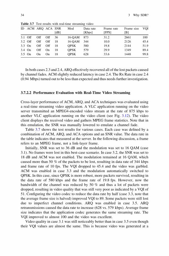
In both cases 2.3 and 2.4, ARQ effectively recovered all of the lost packets causedby channel fades. ACM slightly reduced latency in case 2.4. The Rx Rate in case 2.4(0.94 Mbps) turned out to be less than expected and thus needs further investigation.
3.7.2.2 Performance Evaluation with Real-Time Video Streaming
Cross-layer performance of ACM, ARQ, and ACA techniques was evaluated usinga real-time streaming video application. A VLC application running on the videoserver transmitted an MPEG4-encoded video stream at the rate of 875 kbps toanother VLC application running on the video client (see Fig. 3.12). The videoclient displays the received video and gathers MPEG frame statistics. Note that inthis emulation, the SNR was manually lowered to emulate a channel fade.
Table 3.7 shows the test results for various cases. Each case was defined by acombination of ACM, ARQ, and ACA options and an SNR value. The data rate inthe table indicates that measured at the server. In the following discussion, a framerefers to an MPEG frame, not a link-layer frame.
Initially, SNR was set to 36 dB and the modulation was set to 16 QAM (case3.1). No frames were lost in this best-case scenario. In case 3.2, the SNR was set to18 dB and ACM was not enabled. The modulation remained at 16 QAM, whichcaused more than 50 % of the packets to be lost, resulting in data rate of 344 kbpsand frame rate of 10 fps. The VQI dropped to 45.4 and the video was garbled.ACM was enabled in case 3.3 and the modulation automatically switched toQPSK. In this case, since QPSK is more robust, more packets survived, resulting inthe data rate of 580 kbps and the frame rate of 19.8 fps. However, now thebandwidth of the channel was reduced by 50 % and thus a lot of packets weredropped, resulting in video quality that was still very poor as indicated by a VQI of51. Configuring the video codec to reduce the data rate by half (case 3.3, note thatthe average frame size is halved) improved VQI to 89. Some packets were still lostdue to imperfect channel conditions. ARQ was enabled in case 3.5. ARQretransmissions caused the data rate to increase (628 vs. 579 kbps). Average framesize indicates that the application codec generates the same streaming rate. TheVQI improved to almost 100 and the video was excellent.
Video quality in case 3.1 was still noticeably better than in case 3.5 even thoughtheir VQI values are almost the same. This is because video was generated at a
Table 3.7 Test results with real-time streaming video
ID ACM ARQ ACA SNR[dB]
Mod Data rate[Kbps]
Frame rate[FPS]
Frame size[B]
VQI
3.1 Off Off Off 36 16-QAM 873 31.2 2661 1003.2 Off Off Off 18 16-QAM 344 10.0 2126 45.43.3 On Off Off 18 QPSK 580 19.8 2144 51.93.4 On Off On 18 QPSK 579 29.9 1349 89.43.5 On On On 18 QPSK 628 33.6 1448 99.8
34 3 Why SDR?

lower resolution to achieve a lower data rate, which is reflected in the smalleraverage frame size in case 3.5.
These experiments demonstrated the benefit of multiple, cooperating cross-layer adaptive techniques to mitigate channel effects.
3.7 ACM Case Study 35

Chapter 4Disadvantages of SDR
The advantages of SDR are described throughout this book. The question then is:‘‘Why isn’t every radio already a SDR?’’ No technology is without its disadvan-tages and challenges, and some of them will be discussed in this chapter.
4.1 Cost and Power
The most common argument against SDR is cost. The argument is particularlyimportant for high-volume, low-margin consumer products. Consider a garage orcar door remote opener key fob. This extremely simple device has one and onlyfunction. The mechanical design—a single button—precludes the addition of newfunctionality in the future. Millions of essentially identical devices are sold everyyear, amortizing the development cost of an ASIC. The cost of the ASIC is thenproportional to the size of the chip, which is in turn a function of the chip com-plexity. An SDR chip for garage door openers could be used in many other devicesas well, but the increased market volume would not drive the cost of the chipdown. In fact, since an SDR is necessarily more complex than a single-functionradio, the SDR chip cost would be higher. The same cost argument has been madefor AM and FM radio receivers. These products are also high-volume andpotentially very low cost.1
1 However, AM/FM receivers are often integrated into larger systems (e.g., car audio systems,personal audio players) which require a significant amount of signal processing. If the signalprocessing is already available, the incremental cost of making AM/FM receiver software-basedis small. Moreover, unlike garage door openers, new waveforms are becoming available in theAM/FM channels. New digital radio standards such as HD radio [264] in the US and DAB [265]in Europe provide higher audio quality and new features while coexisting with legacy AM/FM.Unfortunately, since SDR was not used for older receivers, they cannot process new signals.While incompatibility with new waveforms is irrelevant for a one-dollar radio, it is quiteinconvenient for a $400 car stereo.
E. Grayver, Implementing Software Defined Radio,DOI: 10.1007/978-1-4419-9332-8_4, � Springer Science+Business Media New York 2013
37

The second most common argument against SDR is increased powerconsumption. Two sources contribute to higher power consumption in an SDR:increased DSP complexity and higher mixed-signal/RF bandwidth. Power con-sumption in an FPGA or GPP used to implement flexible signal processing iseasily 10 times higher than in an equivalent ASIC.2 Wideband ADCs, DACs, andRF front ends required for SDR consume more power than their narrowbandequivalents. The difference is especially dramatic for wideband power amplifiers,which account for at least 70 % of the total power in a radio. A wideband amplifieris often half as efficient as a narrowband one.3 Power consumption in the ADCsvaries approximately linearly with bandwidth, but is less than linear for DACs.A wideband ADC often also requires higher dynamic range (more bits) to toleratein-band interferers.4 Increasing ADC dynamic range significantly increases thepower consumption [35]. However, waveform adaptation enabled by SDR canreduce the required transmit power; thereby saving power (see Sect. 3.5).
Cost and power consumption arguments are combined when considering theamount of signal processing margin to be included in an SDR. The margin isdefined as the ratio of the DSP horsepower (e.g. measured in FLOPS) provided byan SDR relative to that required for the baseline set of waveforms. For example, anSDR is initially developed to support two waveforms, with the more complex onerequiring 1 GFLOPs. A 100 % margin requires the SDR to provide 2 GFLOPs.It is difficult to predict what waveforms a user may wish to host on an SDR andeven a small underestimate of the margin can preclude the ‘must have’ futurewaveform. Consider some of the early deep space missions that relied on simpleand computationally non-demanding FEC codecs. Thirty years ago the designerscould not imagine the enormous computational requirements of modern iterativecodecs. It would have been (then) unreasonable to include enough DSP margin toenable an upgrade to the powerful codecs of today. Lack of sufficient DSP marginis a very strong argument against the ‘future-proof’ promise offered by SDR.
4.2 Complexity
One generic argument against SDR is the additional complexity it requires. Thecomplexity argument has at least three components:
• Increased time and cost to implement the radio. It takes more engineering effortto develop software and firmware to support multiple waveforms than to support
2 As transistors continue getting smaller, DSP power consumption is becoming an ever smallerpart of the total radio power consumption.3 Development of adaptive impedance matching networks based on MEMS components [267] orvaractors [266] enables wideband tunable power amplifiers. These amplifiers provide a relativelynarrow instantaneous bandwidth which can be tuned over a wide range (also see Sect. 10.4).4 Alternatively, a tunable RF filter is required to remove the interferers. Such filters are not yetavailable.
38 4 Disadvantages of SDR

just one. Some argue that the increase in complexity is super linear (i.e., it takesmore than twice as long to implement a radio that supports two waveforms thanto implement two radios that each support one waveform). This claim is notunreasonable if the radio has to conform to a complex standard such as JTRS(see Sect. 7.1). Specialized expertise required to develop on a particular SDRplatform may disappear soon after the radio is delivered to the customers.Developing new waveforms for that platform in the future can easily be moreexpensive than starting from scratch.5
• Longer and more costly specifications and requirements definition. An SDRdesign has to support a set of baseline waveforms but also anticipate additionalwaveforms. Some DSP resource margin must be provided to support futurewaveforms.
• Increased risk. At least two sources of risk must be considered:
– Inability to complete the design on-time and on-budget due to the concernspresented above. Since SDR is still a relatively new technology, it is moredifficult to anticipate schedule problems.
– Inability to thoroughly test the radio in all of the supported and anticipatedmodes.
Testing SDR is a very active area of research. In the author’s opinion, it is thesingle strongest argument against SDR. How does one test a radio that supports ahuge number of waveforms? It is clearly not possible to test every combination ofsupported parameters (modulations, codes, data rates, etc.). Defining ‘corner’ casesis nontrivial since interaction between components is not obvious (e.g., is theperformance of a tracking loop stressed at low rates or high rates?). Combinationsof FEC block lengths and time constants of adaptive loops introduce a new level ofcomplexity.6 Errors in SDR design can affect not only the faulty radio, but also theentire network. In fact, a wideband SDR could conceivably transmit a signal in anunauthorized band, thereby jamming other life-critical signals.7 Testing an SDR insteady-state (i.e., once a waveform has been selected) is not sufficient. Problemsmay be observed only when switching from one specific waveform to another.
Concerns with security and information assurance problems in an SDR arerelated to the complexity argument. Most modern wireless standards include someform of encryption and authentication. We expect our phone conversations to berelatively immune from interception. The ability to change many aspects of awaveform also implies that the security-related aspects could be changed. It is not
5 The author is aware of at least one system that relied on software tools no longer availabletoday. Even if the old tools could be procured and made to run on modern computers, theengineers with expertise in these tools are hard to find. Clearly, this problem is only a concern forSDRs with long life cycles such as those on satellite payloads.6 The author is aware of one fielded system that exhibited poor performance when the memory ofa FEC decoder happened to be close to the period of phase noise from the front end.7 A bug in the spectrum-sensing block or in the radio constraints database for a cognitive radio(see Sect. 3.4) can make the radio transmit in the GPS band.
4.2 Complexity 39

difficult to imagine a virus that modifies the SDR configuration to disableencryption, or even to have it transmit a copy of the signal at another frequency.These intrusions would be difficult to detect since the user experience is notaffected. The problem is even more important for military radios that handleclassified information. A virus that disables8 all SDRs during a military operationwould be a potent weapon indeed. However, there is nothing special about SDRsecurity and well-understood techniques can be applied to the download of newwaveforms into a radio [36]. The same infrastructure that is currently used forover-the-air distribution of secret keys can be applied to SDR security.
4.3 Limited Scope
Finally, it is important to keep in mind that SDR only addresses the physical layer.The user cannot take advantage of link throughput improvements made possible bySDR without cooperation from upper layers. One example demonstrating the needfor cross-layer adaptation is described in Sect. 3.7.2.2. Another example isdescribed below.
The ubiquitous network protocol, TCP/IP, was developed for fixed-rate chan-nels. A TCP transmitter sends data packets at the highest possible rate. Thereceiver responds with an acknowledgment packet (ACK) as it receives the data. Ifthe transmitter does not get an acknowledgement, the protocol determines that thelink is congested and quickly decreases the data rate. If more acknowledgementpackets are not received, transmitter rate falls even further. The rate increasesslowly once the ACK packets are received once again. Performance of TCP in thecontext of time-varying throughput caused by SDR adaptation to the environmenthas been extensively studied. Results show that end-to-end throughput is muchlower than the physical layer throughput. Moreover, some combinations ofchannel fade rate and TCP settings lead to instability and throughput drops dra-matically. Achieving the average throughput made possible by ACM may alsorequire large buffers at the network routers or in the SDR.
Consider a fixed-rate data source9 with the rate equal to the average physicallayer throughput, Ravg. The SDR supports two waveforms for good and badchannel conditions with rates Rhigh and Rlow. When the instantaneous throughputdrops to Rlow due to a fade, data will start getting backed up. The buffer must belarge enough to hold (Ravg - Rlow) for the duration of the fade, as shown inFig. 4.1.
8 Since FPGAs are used in most SDRs today, a hardware virus may be able to physically damagethe radio by overheating the device [268]. The feasibility of such a virus in modern FPGAs isunknown.9 This discussion does not apply to data sources that can vary the rate based on feedback fromthe physical layer (see, for example, Sect. 3.7.2.2).
40 4 Disadvantages of SDR

Since the fading channel is random, fade duration is theoretically unlimited.The buffer must be sized such that data is not lost more than some specifiedpercentage of the time (e.g., no more than 0.01 %). The average throughput andbuffer size can be derived analytically by assuming a Markov model for transitionsbetween different ACM waveforms [37]. Transition probabilities are derived byanalyzing long-term channel statistics.
Data
Router
Queue (buffer)
SDRRavg Rhigh or
Rlow
time
Que
uele
vel
0
(Ravg – Rlow)×Tfade
Good Bad Good
(a)
(b)
Fig. 4.1 Router buffer size requirement to support ACM. a Conceptual view, b queue levelversus time
4.3 Limited Scope 41

Chapter 5Signal Processing Devices
Transistors are cheap and getting cheaper. This key observation has made SDR areality. A true SDR has to implement at least some of the physical layer func-tionality in software. For the purpose of this chapter the definition is expanded toinclude software-controlled radios. Flexible and programmable digital signalprocessing can be implemented on a wide range of devices. This chapter providesan overview of the different types of devices suitable for implementing the DSPportion of an SDR.
5.1 General Purpose Processors
A general purpose processors (GPP) is a typical microprocessor, like the onespowering personal computers.1 As the name implies, these devices are optimizedto handle the widest possible range of applications. A GPP must perform well forbrowsing the web, word processing, decoding video, scientific computations, etc.The very disparate tasks preclude domain-specific optimizations. GPPs must excelat fixed and floating-point operations, logical operations, and branching. Thismakes them suitable for implementing much of the SDR functionality, startingwith the physical layer DSP and ending with the protocol and network stacks.GPPs provide the easiest development environment and highest developerproductivity. The largest pool of qualified developers is familiar with GPPs.The development tools and expertise apply to GPPs from different vendors andproduct lines. A wide range of operating systems is available, from full featuredgraphical interfaces such as MS Windows to lean real-time products such asVxWorks. These advantages make GPPs the easiest platform for SDR develop-ment as will be discussed in Sect. 6.1.
1 Major vendors include Intel, ARM, AMD, MIPS.
E. Grayver, Implementing Software Defined Radio,DOI: 10.1007/978-1-4419-9332-8_5, � Springer Science+Business Media New York 2013
43
5.2 Digital Signal Processors
A digital signal processors (DSP) is a microprocessor that is optimized fornumber crunching.2,3 Manufacturers of DSP devices can optimize them for amuch narrower set of target applications than GPPs. Power consumption can bereduced by eliminating transistors that a GPP has to devote to sophisticatedcache and peripheral subsystems. The main advantage of DSPs over GPPs is inpower consumption per operation. DSPs come in both fixed- and floating-pointvarieties, with fixed-point versions offering even lower power consumption.DSPs are not well suited for control—(rather than datapath )—intensive codesuch as the protocol and network stack. A typical SDR would pair a DSP with aGPP to implement the network stack.
The development environment for a DSP is somewhat more complex than for aGPP. Operating system support is also significantly more limited, with many DSPprojects not using any OS at all and interacting with the hardware directly. If anOS is required, a real-time one is almost always used. DSP developers are sig-nificantly more difficult to find than GPP developers. Optimal use of a DSPrequires the developer to be very familiar with the internal architecture, and theexpertise in one family does not translate to another family.
DSPs are used extensively in software-defined cellular base stations and inradios that require low power and have modest data rate requirements. In theauthor’s opinion, DSPs are a niche product and do not offer a compellingadvantage over either GPPs or FPGAs.
5.3 Field Programmable Gate Arrays
A field programmable gate array (FPGA) is a microchip that is designed to beconfigured by the user after manufacture. An unconfigured FPGA has absolutelyno functionality.
FPGAs contain programmable logic components called ‘‘logic blocks’’ andreconfigurable interconnect to ‘‘wire’’ the blocks together—somewhat like a one-chip programmable breadboard (Fig. 5.1). Logic blocks can be configured toperform complex combinational functions or simple logic such as AND, NOT,XOR, etc. Each logic block is usually paired with one or more registers to store theresult. Most FPGAs also include large ‘‘macro blocks’’ for frequently used func-tions such as memory blocks, multipliers, interfaces to external devices, and evencomplete microprocessors. The macro blocks could be usually built up from thelogic blocks, but the resultant design would be slower and use up a lot of the
2 Major vendors include Texas Instruments, AMD, Free scale.3 There is unavoidable acronym confusion when discussion digital signal processors (DSP) usedfor digital signal processing (also DSP). The second meaning is used more frequently.
44 5 Signal Processing Devices

available logic blocks. FPGA vendors attempt to differentiate themselves byproviding the right mix of logic and macro blocks.4
The interconnect can be used to implement the desired functionality. Forexample, a few gates can be combined to implement an adder, while a few moreimplement a multiplier. However, the overhead of all the wiring and switchesmakes FPGAs consume significantly more power (109) than an equivalent single-function design. Designs implemented on an FPGA also execute a lot slower (59)than an equivalent single-function design [38].
Three types of FPGAs can be defined based on the way they are configured:
1. SRAM-based FPGAs use volatile memory registers to configure the routingbetween logic elements and the detailed logic element implementation. The
RAM RAM
Power PC
I/O I/O
Fig. 5.1 Conceptual block diagram of an FPGA, note the programmable interconnect usingcross-bar connections
4 For example, a high-end FPGA from Xilinx in 2011 (XCE7V200T) provides the following setof blocks. Vendors are still experimenting with providing complete microcontrollers as dedicatedblocks inside an FPGA.
Logic gates Registers RAM blocks Multipliers(w/adders)
Gigabittransceivers
Clock generators
2 M 2.5 M 6 MB 2,100 36 24
5.3 Field Programmable Gate Arrays 45

configuration is lost if power is removed and must be reloaded every time thedevice is powered up. Note that this implies that external, non-volatile memoryis required to use SRAM-based FPGAs. The external memory may reside onthe same circuit board, or could be on a hard disk 1,000 miles away, but theconfiguration data have to be loaded. The volatile memory registers are verysmall and leave a lot of room on the FPGA chip for logic elements and routing.Thus, all large FPGAs are SRAM-based and account for most of the FPGAmarket. The two dominant vendors, Xilinx and Altera, account for 90 % of allFPGA sales [39]. Their products are quite similar,5 with Xilinx providingslightly larger devices at the time this book is written. Xilinx devices are alsoslightly better supported by IP vendors.
2. FLASH-based FPGAs use non-volatile memory registers instead of the volatileones. One advantage is that the FPGA is ready to process data as soon as poweris applied; no external NV memory is required. The NV registers consume nopower resulting in lower idle power consumption (by as much as 29). How-ever, FLASH registers implemented in standard silicon processes used to makeFPGA logic are much larger than SRAM registers. The configuration registersleave less room on the chip for user logic.6 FLASH registers are more robust toradiation effects [40], which is a major concern for the aerospace industry.Some SRAM-based FPGAs include FLASH memory either in the samepackage (e.g. Xilinx Spartan-AN) or even on the same die (e.g. Lattice XP2).However, such devices do not have the radiation tolerance advantages of a trueFLASH FPGA. The only FLASH FPGA vendor is Microsemi (previouslyActel) [41].
3. Antifuse-based FPGAs rely on unique chemical switches between interconnects.These switches are normally open, but can be closed by passing current throughthem. Once closed, the switch cannot be opened again. Thus, antifuse FPGAscan be programmed only once. Antifuse-based FPGAs are therefore not suitablefor SDR implementation because the functionality cannot be changed. Onceprogrammed, they should be considered ASICs. Antifuse switches are evenlarger than FLASH configuration registers, leaving little room for user logic.7
Antifuse FPGAs are used almost exclusively by the aerospace industry becauseof high radiation tolerance. The only antifuse FPGA vendor is Actel [42].
To the best of the author’s knowledge, only SRAM-based FPGAs have beenused to implement SDRs for both terrestrial and space8 use. The high signal
5 Each vendor has a devoted following who would disagree with this statement.6 The largest flash FPGA in 2011 is the Actel RT3PE3000L with approximately 75 K registers.Compare that to the 2.5 M registers in a top-of-the-line SRAM FPGA.7 The largest antifuse FPGA in 2011 is the Actel RTAX4000S with approximately 10 Kregisters.8 A radiation-tolerant antifuse FPGA is used to control and configure the SRAM FPGAs inspace-based SDRs. SRAM FPGAs are used for all the signal processing. A new radiation-tolerantSRAM FPGA was recently developed by Xilinx and the US Air Force [263].
46 5 Signal Processing Devices

processing requirements of a modern SDR simply exceeds the capabilities ofFLASH devices.
The ability to implement exactly the functionality required for the radio9
without any unused logic makes FPGAs dramatically more efficient than GPPs.FPGAs excel at heavy-duty number crunching in a datapath flow, but are not
as well suited for control-intensive processing. A microcontroller is often imple-mented using some of the logic gates or an external microcontroller is paired withthe FPGA. The microcontroller is then used for the control-intensive processing.The development flow and environment for an FPGA are very different from thoseused for DSP or GPP (see Sect. 11.3).
5.4 Specialized Processing Units
A number of devices suitable for DSP do not fall neatly into any of the categoriesabove. These are referred to as SPUs and will be called out by name whennecessary. Specialized processing units (SPUs) typically combine multiple coreswith different characteristics to allow efficient mapping of SDR algorithms. Aninteresting overview of some modern SPUs developed specifically for SDR isprovided in [43].
The GPP used to be the most complex and powerful chip in a PC. Today thegraphics processor (GPU) responsible for displaying images on the screen is oftenmore complex than the GPP. Image processing can be expressed as a set of linearalgebra operations. Much of the signal processing required for the physical layer ofan SDR can be expressed using similar operations. A GPU is essentially an arrayof floating-point multipliers with efficient access to memory and can be considereda very specialized DSP. In terms of raw performance (GFLOPs), and single GPUoutperforms a GPP by a factor of at least 5 and a DSP by a factor of 3. Theincreased specialization makes them more efficient but more difficult to program.GPU vendors have realized the potential new market for their chips and each newgeneration is becoming easier to program for non-imaging applications. Generalpurpose GPUs (GPGPUs) are slightly tweaked GPUs marketed to high-perfor-mance computing users.
The most mature GPGPU programming language, CUDA, is developed byNVIDIA [44]. An open source language, OpenCL, is gaining ground [45, 46].Writing software to take advantage of these devices remains very challengingbecause of non-intuitive interaction between processing elements and memory.Optimized function libraries can be used to take advantage of GPGPUs from
9 The designer can choose to use either fixed- or floating-point logic, at any precision. Forexample, if the input data is only 1 byte (8 bits) a GPP still has to use the 64-bit adder to processthe data. In contrast, an FPGA can be configured to implement an 8-bit adder, making it moreefficient.
5.3 Field Programmable Gate Arrays 47

popular development environments such as MATLAB and C ++ without having toprogram in CUDA of OpenCL (e.g. [47]).
An obvious question is: If GPUs are so fast, why are there no similar devicesoptimized for SDR instead of video processing? The answer is cost. GPUs arerelatively inexpensive because of the huge volume—a lot more people are buyinghigh-end video cards for gaming than are buying SDRs. Since SDR is still arelatively small market, it has to either use general purpose devices (GPP, DSP,FPGA) or repurpose devices developed for larger markets.
The IBM Cell processor [48] is another device that has been successfully usedfor SDR development. Cell was developed for image processing required for videogames. However, the architecture was developed from the ground up to supportapplications other than video games. Unlike GPUs, a Cell processor includes a fullfeatured GPP in addition to an array of specialized DSPs (synergistic processingelement, SPE). The Cell processor also offers lower power consumption perGFLOP than a GPU. However, since GPUs are sold in much larger volumes, theCell processor is much more expensive.10 A robust general purpose (rather thangraphics specific) development environment was available for the Cell from thebeginning. This made it an attractive target for HPC and even motivated a versionof the popular open source SDR framework (GNURadio, see Sect. 8.1).
Fig. 5.2 SODA processor architecture [50]
10 The only inexpensive Cell processor system is a Sony PS3 because it is subsidized by themanufacturer.
48 5 Signal Processing Devices
The SODA architecture [49] (and the derived Ardbeg chip) was designedspecifically for SDR [50]. This chip can be considered a scaled down version ofthe Cell processor with a GPP augmented by four SIMD cores. The Ardbeg chipwas never released commercially. The architecture, shown in Fig. 5.2, is repre-sentative of a class of SIMD-augmented processors. A nice summary of Ardbegfeatures and comparison to similar processors is provided in [50].
A host of other devices developed for flexible signal processing can be used toimplement an SDR. There is an interesting intersection between chips targeted atthe SDR and the HPC markets. Both markets are rather small and somewhatcrowded with established players. This makes new entrants likely to fail, andmakes adoption of these new devices risky. The specialized nature of new devicesimplies a significant learning curve to effectively use the resources and thedevelopment flow. Investment in time has to be carefully weighed against theadvantages of the device given the risk of it disappearing in a year or two [51].Some of the notable failures in the last decade include: morphX, mathchip,sandbridge [52, 53]. Some of the remaining entrants are:
• Coherent Logic’s HyperX, which claims to offer both low-power consumptionand high-computational throughput [54]. The architecture is somewhat similarto that of a GPU.
• Octasic offers a multi-processor solution with each processor derived from aDSP (rather than a GPP) [55].
• picoChip11 offers arrays of up to 273 primitive DSPs [56].• Tilera offers yet another massively multi-processor device [57]. The Tile pro-
cessor is representative of the other devices mentioned above and will be dis-cussed in more detail below.
5.4.1 Tilera Tile Processor
The trend in both high-performance and low-power computation is to integratemultiple processor cores on a single die. Simply increasing clock rates has becomeinfeasible, mostly due to heat dissipation issues. Modern high-performanceprocessors offer 6 or more fully functional cores on a single die. The embedded,low-power processors are pushing the number much higher. Tilera markets a64-core device, which is about half way between the 4? core Sandbridge and the270? core picoChip. As mentioned previously, many of the companies offeringnovel processor architectures are very short lived. The Tile64 processor fromTilera received a strong vote of confidence from the military space community
11 As this book went to print, picoChip was acquired by Mindspeed Technologies and the futureof its products is uncertain.
5.4 Specialized Processing Units 49

when Boeing was commissioned to develop a space-qualified version [58]. Theradiation hardened by design (RHBD) version of Tile64 is called MAESTRO.Space-qualified chips have much longer life cycles than their terrestrial equiva-lents. A payload designed around the MAESTRO chip may take 5 to 10 years tocomplete and launch. Radiation hardening is very expensive and the few chips thatare available get used for multiple programs. Entire sessions at multiple space-related conferences are now devoted to the MAESTRO chip [59, 60]. Developerscan feel relatively confident that software tools will remain available even if Tileradoes not succeed in the marketplace.
The MAESTRO chip is built around a 7 9 7 array of processors,12 known astiles, as shown in Fig. 5.3. The 49 tiles share access to four memory interfaces andfour high-speed serial interfaces. Each MAESTRO tile is a three-way VLIWprocessor with 8 kB L1 data cache, 64 kB data/instruction cache, a DMA engine,
switch
caches
7×7array of
processors(tiles)
XAUI10 Gbps
XAUI10 Gbps
I2C
UART
HPI
SPI
DDR2 RGMII DDR2
DDR2 RGMII DDR2
XAUI10 Gbps
XAUI10 Gbps
GPIO
JTAG
Clock
Reg File
P2
P1
P0
processor
L2 Cache
L1I L1D
2D DMA
MDN TDN
UDN IDN
SDN
(a)
(b)
6 on-chipnetworks
6on-chip
n etworks6
on-c
hip
netw
orks
Flo a
ting
p oi n
tun
it
Fig. 5.3 MAESTRO chiparchitecture a top level,b detail of one tile
12 Note that it is smaller than the commercial counterpart. Commercial Tile processors do nothave a floating-point unit.
50 5 Signal Processing Devices
4

and a floating- point unit. Each tile uses about 200 mW when running at 300 MHz.The peak performance for the entire chip is 44 GOPs and 22 GFLOPs.
Tiles are interconnected in a two-dimensional mesh with five high-speed, lowlatency networks between every four tiles (and one system network). Each tileincludes a switch to route packets. Note that latency increases linearly with thedistance between the source and destination tile for a packet. Software algorithmsshould therefore be designed to minimize data transfers between non-adjacenttiles.
One of the main strengths offered by Tilera is ability to run standard Linux andVxWorks operating systems. This means that porting an SDR framework such asGNURadio (see Sect. 8.1) to Tile64 is relatively straightforward. A direct portwould not make efficient use of the cores, but allows gradual optimization.Mapping each SDR functional block to one or more adjacent tiles is a simpleoptimization step. However, best performance can only be achieved by leveragingthe hand-optimized libraries provided by Tilera.
5.5 Application-Specific Integrated Circuit
Application-specific integrated circuit (ASICs) are not typically mentioned in thecontext of SDR, but remain a viable alternative for very flexible radios.13 An ASICcan be used to implement a software-controlled radio. ASICs power most oftoday’s cell phones and other handheld devices and allow them to support multiplewaveforms. The ASICs in cell phones implement a system-on-a-chip (SoC) withone or more GPPs and DSPs in it. The most numerically intensive functionalblocks are implemented in dedicated circuits or accelerators, while the rest of theprocessing is done in software. ASIC development flow is quite similar to FPGAdevelopment flow, with additional steps required for the final manufacture.
5.6 Hybrid Solutions
As transistor density keeps increasing, manufacturers can put multiple devices on asingle chip. A number of hybrid devices are available that combine two or more ofthe processors described above. One of the first commercially available exampleswas the OMAP architecture from Texas Instruments. An OMAP chip combines aGPP with a DSP [61].14 The ZYNQ family of devices from Xilinx combines
13 Technically, all of the processor types described above are themselves ASICs (i.e., an FPGAis a large ASIC that happens to be programmable).14 The GPP/DSP architecture has been abandoned by TI in favor of multiple GPPs and dedicatedhardware accelerators.
5.4 Specialized Processing Units 51
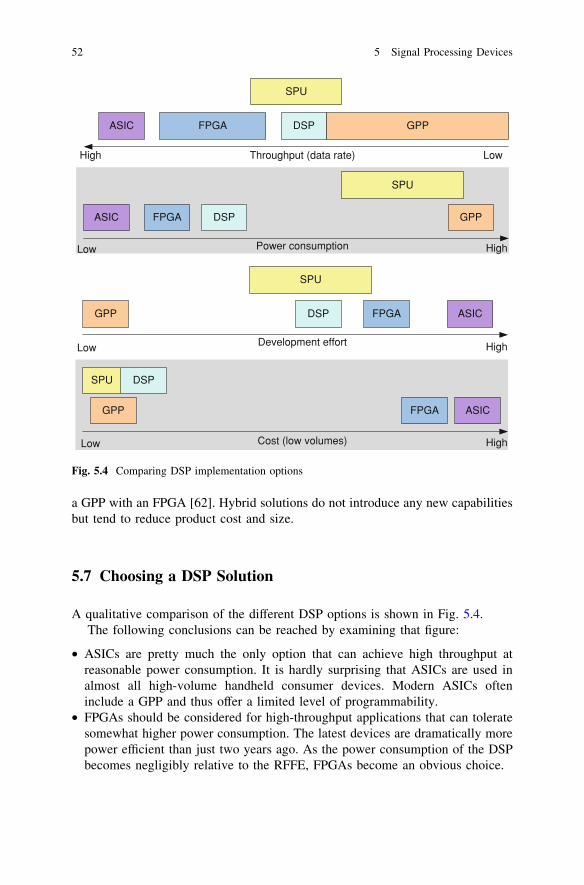
a GPP with an FPGA [62]. Hybrid solutions do not introduce any new capabilitiesbut tend to reduce product cost and size.
5.7 Choosing a DSP Solution
A qualitative comparison of the different DSP options is shown in Fig. 5.4.The following conclusions can be reached by examining that figure:
• ASICs are pretty much the only option that can achieve high throughput atreasonable power consumption. It is hardly surprising that ASICs are used inalmost all high-volume handheld consumer devices. Modern ASICs ofteninclude a GPP and thus offer a limited level of programmability.
• FPGAs should be considered for high-throughput applications that can toleratesomewhat higher power consumption. The latest devices are dramatically morepower efficient than just two years ago. As the power consumption of the DSPbecomes negligibly relative to the RFFE, FPGAs become an obvious choice.
Throughput (data rate)
Development effort
ASICFPGADSP
SPU
GPP
Power consumption
ASIC FPGA DSP
SPU
GPP
Cost (low volumes)
ASICFPGA
DSPSPU
GPP
ASIC FPGA DSP
SPU
GPP
High Low
HighLow
High
High
Low
Low
Fig. 5.4 Comparing DSP implementation options
52 5 Signal Processing Devices

• GPPs can now process low- to-medium throughput signals in real time. Theyoffer unmatched flexibility and ease of development. GPPs should be the firstchoice for SDRs when power consumption is not a major concern.
• DSPs are definitely niche devices. They do not offer sufficiently higherthroughput or lower power than alternative options. They are used when GPPsare either not fast enough or consume too much power and the developmentteam does not have FPGA expertise.
• SPUs must be considered on a case-by-case basis. The two key concerns whenconsidering SPU are device longevity and ease of development.
Three major signal processing architectures can be defined based on Fig. 5.4:
• All-software using a GPP• GPP with hardware acceleration using an FPGA or SPU• FPGA
Note that the DSPs are not used in any of these architectures. This omission ispartly due to the author’s bias against DSPs—they are only marginally easier towork with than FPGAs and almost always offer lower performance (for aninteresting comparison, see [63]). The optimal architecture depends on manyfactors, including:
• Expected signal processing requirements (in operations per second15)
– The bandwidth of the signal(s) to be processed is a rough indicator of therequired signal processing. A wideband signal is either high data rate orhighly spread. In the first case, the FEC will require a lot of processing, whilein the second case the DSSS acquisition will.
• Number of signals. Assuming all the signal(s) of interest are digitized together,rather than separated in the RF front end, the DSP has to handle the entirebandwidth before separating the signals for individual processing. Wide inputbandwidth makes it difficult or impractical to use a GPP for initial channeli-zation. On the other hand, it is more difficult to develop FPGA firmware tosimultaneously support multiple narrowband signals than a single widebandsignal.
• Operating environment. All of engineering is about achieving the desiredgoal given a set of constraints. The constraints for an SDR radio used in aresearch/lab environment are very different from those for a handheld con-sumer device. Three classes can be defined to express different targetenvironments:
15 An operation can refer to a floating point, fixed point, or bit operation. A GPU/SPU/DSP useswhatever arithmetic and logic unit (ALU) is available for each operation, while an FPGA canimplement each operation in a dedicated circuit. Thus, comparing the DSP capabilities based onGFLOPs or GMACs is only often misleading.
5.7 Choosing a DSP solution 53

• Flexibility and responsiveness. A consumer device may never need to changethe supported waveforms after it has been shipped, or the updates may comeonce a year. Conversely, a research SDR may require different waveforms to beimplemented on a weekly basis. The level of effort and manpower required toimplement changes can be a deciding factor.
• Available skill set. If multiple architectures satisfy the ‘hard’ constraints, the finaldecision frequently hinges on the development team’s skill set. A longer termview should also take into account the ease of bringing new/additional devel-opers into the group. A single expert16 in a unique device or tool chain can steer agroup down a path that results in a steep learning curve and lost productivity.
• Maintainability. A development effort with a well-defined end date and finalgoal can take advantage of the current state-of-the-art devices. However, a long-term strategic development effort must consider how the selected device willevolve over time. An SPU from a small start-up can be a perfect fit for the taskat hand, but may not offer a clear evolutionary path. Likewise, development forthe current FPGA must consider how the unique capabilities offered by thatdevice may limit the value of the developed codebase once the next generationof the FPGA is available.17
– The GPP is indisputably the best platform for maintainability. Well-written18
C++ or Java code from 20 years ago can still be compiled today.
Size Power Cost
Rack Size is essentially unconstrained Power is essentiallyunconstrained, only limited byheat dissipation to \10 kW
Cost is not adriver
Desktop Size is constrained to a volume ofabout 1 m3—a large PC tower ortest instrument.
Power is constrained to asingle outlet \1 kW
Handheld Size is a key design driver andshould be as small as possible, butno larger than 100 cm3.
Power is just as important assize, limited to \1 W onaverage
Cost is sensitivefor high-volumedevices.
16 This problem is especially acute in large corporations with a lot of institutional knowledge.See the discussion of SPW and Simulink in Chap. 11.17 Maintainability and ease of upgrades are strongly affected by the development toolset. Thehigher the abstraction level, the easier the upgrade path … unless the toolset used to convert fromabstract description to the implementation disappears. See the discussion of design flows inChap. 11.18 Unfortunately, writing portable code often means eschewing the use of optimizedperformance libraries, since the libraries may not be available or may change significantly inthe future.
54 5 Signal Processing Devices

Chapter 6Signal Processing Architectures
One or more devices described in Chap. 5 can be used to implement an SDR. Thischapter considers SDR architectures based on each DSP option. The receiver in anSDR almost always requires significantly more computational resources than thetransmitter. Thus, only receiver architectures will be discussed in this chapter.
6.1 GPP-Based SDR
A GPP-based SDR offers maximum flexibility and the easiest development. GPPsare best suited for SDRs used in a laboratory environment for research anddevelopment, because size and power consumption are not significant concernsand the ability to quickly try out a range of algorithms and waveforms is critical.1
The maximum data rate that can be supported on a high-end PC in 2010 was about1 Mbps for a reasonably complex waveform (see Sect. 8.1.4 and [64]). This datarate can be achieved without heroic measures by parallelizing the signal pro-cessing. The PC receives digitized baseband or low-IF samples over one of thestandard interfaces (Ethernet, USB, FireWire, PCI). The samples are buffered andpassed to the signal processing threads.
Latency is a major concern for GPP-based SDRs. GPPs achieve high perfor-mance only when working on blocks of data, rather than on one sample at a time.2
The operating system also introduces latency and jitter when handling interruptsand context switching for different threads. The jitter can exceed 10 ms on aWindows system but a real-time operating system such as VxWorks can achieve
1 Real-time operation is assumed. A nonrealtime (offline) software-defined radio is bestcharacterized as a simulation platform.2 A single-instruction-multiple-data (SIMD) floating point unit is available on modern GPUsfrom Intel and AMD. It can perform the same operation on up to eight samples at once. However,overhead to set up the SIMD transaction is only justified for blocks larger than 128 samples. Inpractice, blocks of thousands of samples are used to reduce overhead. Note that very large blocksthat exceed the cache size cause performance to drop.
E. Grayver, Implementing Software Defined Radio,DOI: 10.1007/978-1-4419-9332-8_6, � Springer Science+Business Media New York 2013
55
m

jitter below 1 ms. Jitter and latency due to the digitizer interface must also beconsidered––under 10 ls for 10 GbE [65], under 100 ls for 1 GbE [66], up to200 ls USB [67]. Jitter and latency become a major concern if the waveformrequires the transmissions to be scheduled based on received data. Manycommercial standards (e.g. WiMAX, UMTS) place this requirement, and theturn-around time is often tight (\10 ms). If the latency from the digitizer to thesoftware running on the GPP exceeds half3 of the turn-around time, the waveformcannot be supported. Likewise, if the jitter exceeds half of the uncertainty window,the waveform cannot be supported. An example showing the effect of latency ispresented in Fig. 6.1. A downlink packet is transmitted at a slot boundary in aTDMA system (see Sect. A.5.1). It is received by the GPP after L seconds due tolatency. Some time, C, is required to process the received packet and generate aresponse. The response packet reaches the antenna another L seconds later andmisses the start of the time slot.
The effect of jitter is shown in Fig. 6.2. In this scenario, latency is small enoughto give GPP plenty of time to prepare the uplink packet. Uplink is started Lseconds before the uplink time slot. On average, the uplink packet will be
Downlink packet
Downlink packet
L L
Uplink packet
C
Uplink Packet
time
Uplink must start at this time
GPP
viewR
Fview
Fig. 6.1 Missing the uplink slot due to excessive latency
Downlink packet
Downlink packet
L
Uplink packet
C
Uplink Packet
L
J
J
2J
GP
Pview
RF
view
time
Fig. 6.2 Missing uplink slot due to excessive jitter
3 Latency is incurred when receiving and again when transmitting the response.
56 6 Signal Processing Architectures

transmitted at the correct time. However, the combined receive and transmit jitter,2J, may cause the start of the uplink packet to fall outside the allowed uncertaintyrange (i.e. it could start J seconds earlier or later than desired).
Some waveforms require accurate synchronization to absolute (e.g. GPS) timerather than to the received signal. For example, a spreading code in a DSSSwaveform can be a function of GPS time (see Sect. A.5.5). The code cannot beacquired without knowing the time, and the acquisition complexity grows linearlywith time uncertainty. Relatively accurate time4 can be acquired on a PC usingeither a dedicated GPS-based timing card, or network-based synchronization toolssuch as NTPv4 [68] or IEEE 1588 [69]. However, the accuracy is still limited bythe jitter of the digitizer to PC interface. The digitizer can be configured to addtimestamps to the data samples, as shown in Fig. 6.3. The timing accuracy is thenonly limited by the digitizer hardware and can be made very accurate (�1 ls) ifthe digitizer has access to GPS time and a 1 pulse per second signal.5 Accuratescheduling of transmissions can be greatly simplified if the hardware is responsiblefor starting the transmission. The hardware has to have a buffer to hold samples
A/D
Insert TS every N samples
TS
N data samples
TS
FIFO
M M data samplesTS
TS
M
D/A
=
Zero
Digitizer GPP
Process downlink packet
Compute start time(s) for uplink
packet
Generate uplink packet (s)
Send M samples from FIFO after TS matches current time
Fig. 6.3 Possible implementation of a time-aware mixed-signal front end for a GPP-based SDR(TS indicates a timestamp)
4 A well implemented IEEE 1588-2008 on a Linux machine with a time server.5 Access to the absolute (e.g. GPS) time is usually not required. A 1 PPS signal can be used tosimultaneously reset a free-running counter and any internal buffers. The GPP can then correlatethe local time acquired by any means with received data samples. Local time has to be accurate to1 s. Software uses the nominal sample rate to compute the time of arrival for the Nth sample.
6.1 GPP-Based SDR 57
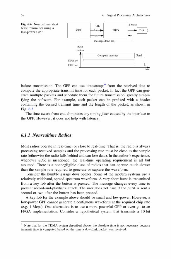
before transmission. The GPP can use timestamps6 from the received data tocompute the appropriate transmit time for each packet. In fact the GPP can gen-erate multiple packets and schedule them for future transmission, greatly simpli-fying the software. For example, each packet can be prefixed with a headercontaining the desired transmit time and the length of the packet, as shown inFig. 6.3.
The time-aware front end eliminates any timing jitter caused by the interface tothe GPP. However, it does not help with latency.
6.1.1 Nonrealtime Radios
Most radios operate in real-time, or close to real-time. That is, the radio is alwaysprocessing received samples and the processing rate must be close to the samplerate (otherwise the radio falls behind and can lose data). In the author’s experience,whenever SDR is mentioned, the real-time operating requirement is all butassumed. There is a nonnegligible class of radios that can operate much slowerthan the sample rate required to generate or capture the waveform.
Consider the humble garage door opener. Some of the modern systems use arelatively wideband, spread-spectrum waveform. A very short burst is transmittedfrom a key fob after the button is pressed. The message changes every time toprevent record-and-playback attack. The user does not care if the burst is sent asecond or two after the button has been pressed.
A key fob for the example above should be small and low-power. However, alow-power GPP cannot generate a contiguous waveform at the required chip rate(e.g. 1 Mcps). One alternative is to use a more powerful GPP or even go to anFPGA implementation. Consider a hypothetical system that transmits a 10 bit
GPP FIFOdata D/A
wr
message done (rd)
1 kHz 2 MHz
time
pushbutton
Compute message Send
FIFO wr
FIFO rd
Fig. 6.4 Nonrealtime shortburst transmitter using alow-power GPP
6 Note that for the TDMA system described above, the absolute time is not necessary becausetransmit time is computed based on the time a downlink packet was received.
58 6 Signal Processing Architectures

message at a rate of 1 Kbps, spread with a 1 Mcps code. The duration of themessage is 10 ms = 10,000 chips = 20,000 samples (assuming 2 samples/chip).A low-power GPP can compute the required samples and put them into a 20 kB(assuming 8 b/sample) FIFO7 at some arbitrarily low rate (e.g. 1 kHz). Once themessage is complete, the FIFO can be read out at the required 2 MHz rate, asshown in Fig. 6.4.
Design of a low-power nonrealtime receiver is less obvious. The transmitterwas started by the user pressing a button. A typical receiver has to be always activesince the message can arrive at any time.8 One option for nonspread waveforms isto rely on a passive power detector to start capturing the signal. However, the SNRfor a spread signal is too low to trigger a power detector. A nonrealtime transceiveris also suitable for battery assisted passive (BAP) RFID tags [70]. Incident RFenergy from the interrogator, captured by a passive energy detector, is used towake up the transceiver (Fig. 6.5). Once awake, the receiver captures a block ofsamples into a FIFO. A low-power GPP can then process the captured samples atlow speed. The transmitter operates similar to the example above, with the receiverproviding the trigger instead of the push button.
Energydetector
time
Detectenergy
Demodulate and process messageCapture
FIFO wr
FIFO rd
A/D FIFOdata GPP
2 MHz 1 kHz
rdwr
power
StartTX
data
Fig. 6.5 Non-realtime short burst receiver using a low-power GPP
7 Some microcontrollers have enough on-chip memory to implement this FIFO. Themicrocontroller would also have to provide a synchronous external interface that can be directlyinterfaced to a DAC chip.8 Some wireless systems define regular intervals at which the receiver must be woken up tocheck if a signal is present (e.g. every minute, on the minute). This approach requires the receiverto keep track of absolute time.
6.1 GPP-Based SDR 59

6.1.2 High-Throughput GPP-Based SDR
Throughput of a GPP-based radio can be increased by dividing the signal pro-cessing among many GPPs. A cluster of GPPs must be interconnected with highspeed links. This solution is clearly only applicable for large ground stations orlaboratory experimentation since both the size and power consumption are veryhigh. An experimental radio reported in [71] supports signals with up to 40 MHzof bandwidth, at least an order of magnitude higher than a single GPP.
6.2 FPGA-Based SDR
An FPGA-based SDR can support high data rates and high bandwidth waveformsin a relatively compact and low-power package. At the time this book was written,high-end FPGAs provide enough signal processing resources to support mostpractical waveforms in a single device. Multiple devices may be required for anunspread waveform with a bandwidth above 300 MHz or a spread waveform witha large acquisition space.9 Low-end FPGAs are suitable for bandwidths from10 MHz down to 100 kHz, and provide much lower power consumption than theirhigh-end counterparts. Although FPGAs can be used to process narrowbandwaveforms below 100 kHz, other devices such as DSPs and GPPs may be a betteralternative.
As discussed previously, FPGAs are fundamentally different than GPPs. A GPPexecutes instructions from memory and can easily switch from one function toanother. Additional functions do not slow down the processor or require moreresources.10 An FPGA has all the functionality mapped to dedicated circuitry, andeach new function requires more FPGA resources. Despite this difference, FPGAscan be used to implement very flexible radios and support a wide variety ofwaveforms. There are four ways (discussed in next subsections) to support dif-ferent waveforms on an FPGA:
1. Create separate configuration files for each waveform and load them as needed.2. Develop the firmware to support all the waveforms in a single configuration.3. Develop a small set of configurations to support different waveform classes and
support multiple waveform variations within a class.4. Take advantage of partial reconfiguration offered by some FPGA devices to
load only the difference between waveforms.
9 The DSSS acquisition problem can be made arbitrarily difficult by extending time and/orfrequency uncertainty..10 Other than memory to store the instructions, which can often be neglected.
60 6 Signal Processing Architectures

6.2.1 Separate Configurations
Unlike a GPP, it takes time for an FPGA to load a new configuration.11 A largeFPGA can take over 100 ms to load.12 The configuration files are also quite large,up to 40 MB per configuration. Reloading the FPGA causes it to lose all stateinformation, and an external memory is required if data must be saved betweendifferent configurations. This approach gives the designer the greatest flexibilityfor designing firmware to target a specific waveform. All the FPGA resources areavailable for just that waveform, making the best use of the FPGA. However, thenumber of configurations can quickly become impractical.
6.2.2 Multi-Waveform Configuration
The firmware is designed to support all the expected waveforms. Unique featuresof every waveform are selected by setting appropriate registers at run time. Thisapproach places a much greater burden on the developer and makes the codesignificantly more complex. For example: a continuously variable resampler isrequired to support different data rates; tracking and acquisition algorithms mustsupport different waveforms; etc. Implementation of FEC codecs for differentalgorithms is typically so different that a dedicated implementation is required foreach.13 FEC decoders are typically the most complex and resource intensiveblocks in a radio receiver, and having dedicated implementations for each canexceed the available resources on an FPGA. Runtime reconfigurable logic isalways slower than single-function logic. Thus, firmware designed to supportmultiple waveforms achieves lower throughput.
The major advantage of this approach is the ability to switch between wave-forms almost instantaneously. Rapid reconfiguration is required for some wave-forms (see the discussion of ACM in Sect. 3.1.1). Another potential advantage isthat the firmware for a multi-waveform configuration can be retargeted from anFPGA to an ASIC. An ASIC implementation is justified if the SDR is used in ahigh volume, low power, and cost-sensitive product.
Many waveforms are very similar to each other, and only minimal changesare required to the firmware for one to support the others. For example, if the
11 An interesting FPGA architecture from Tabula [286] reconfigures the FPGA almostinstantaneously. However, the reconfiguration is not under user control and is meant forresource reuse rather than real-time functionality change.12 Virtex XC7V1500T requires about 40 MB of configuration data and can be loaded over a 32-bit bus at 60 MHz.13 Reconfigurable codecs can be developed to cover some algorithms [281].
6.2 FPGA-based SDR 61

data rate changes between two waveforms, a simple decimator/interpolator isrequired.14 An interpolator uses few FPGA resources and is easy to implement.On the other hand, a GSM waveform shares almost nothing with a WiMAXwaveform. Grouping waveforms into classes based on similarity of signal pro-cessing motivates a hybrid approach with each configuration supporting an entireclass of waveforms.
6.2.3 Partial Reconfiguration
Some FPGAs15 allow only part of the device to be reconfigured, while the rest ofthe device continues operating. This technique is known as partial reconfiguration(PR) [72] and has been available to designers for almost a decade. Unfortunately,the implementation of this approach is rather difficult and suffers from limiteddevelopment tool support. It is easy to come up with plausible applications ofpartial reconfiguration, but the advantages are less compelling than they firstappear.
Partial reconfiguration supported by Xilinx is coarse grained––i.e. relativelylarge sections of the device have to be reconfigured at once. At one extreme, PRreduces to the separate configurations approach, with only a small section of theFPGA retained between configurations. A major main advantage of ‘almostcomplete reconfiguration’ is that an external processor is not needed to manage theconfigurations. Instead, an embedded processor is used. The embedded processoris also responsible for retaining state information from the reconfigured region.
Partial reconfiguration fits well with hybrid FPGA/GPP architectures (seeSect. 6.5) as well as with hardware accelerated architectures (see Sect. 6.6). Theexcellent work in [73] provides a mathematical framework to schedule the loadingof reconfigurable segments onto an FPGA to accomplish the desired computation.
SDR is an application always mentioned by FPGA vendors when touting PRfeatures of their latest devices. The next few pages explore a few specific examples[74].
6.2.3.1 Partial Reconfiguration for ACM
A radio using adaptive coding and modulation (ACM) (see Sect. 3.1) choosesdifferent waveforms to efficiently use available spectrum under varying channelconditions. Partial reconfiguration appears to be an elegant solution for supporting
14 For example, the WiMAX standard defines essentially the same waveform for channelbandwidth of 3.5, 5, 7 and 10 MHz.15 Both major vendors, Altera [283] and Xilinx [282], support this technique..
62 6 Signal Processing Architectures

fast ACM in small FPGAs. Consider an FPGA partitioned into one fixed regionand two reconfigurable regions as shown in Fig 6.6.16
Figure 6.7 shows one possible scenario where the receiver is initially config-ured for a high-throughput waveform. The transmitter, implemented in the fixedregion of the FPGA, sends channel SNR updates to the other radio. When the SNRdecreases, the ACM algorithm executing on the other radio initiates a waveformchange. The waveform change command is processed by the ACM block (in thefixed region of the FPGA). ACM block then initiates reconfiguration. The firstregion is reconfigured to implement a demodulator for a robust waveform (BPSK).The second region is reconfigured to implement a more powerful and lower rateFEC decoder.
Consider a fast-ACM system in which every frame carries a preamble toindicate the code and modulation (CMI) used in the payload (see Sect. 3.1.1). It iscritical that the time required to reconfigure the FPGA and then process a frame ofdata is less than duration of two frames. Incoming data are buffered while the CMIis parsed in the fixed region. Logic in the fixed region or an external GPP thenloads configuration into RR1 to process CM1. Once CM1 is loaded, buffered dataare processed. In the meantime, CMI for the second frame has been parsed by thefixed region and RR2 is loaded. The pipeline continues with sufficient throughputto support contiguous data (Fig. 6.8).
ReconfigRegion 1
ReconfigRegion 2
Fixe
dR
egio
n
Fig. 6.6 FPGA with onefixed and two reconfigurationregions (RR)
16-QAM demodulator
Viterbi (r=¾) decoderT
XBPSK
demodulator
LDPC (r=¼) decoderT
X
(a) (b)
AC
M
AC
M
Fig. 6.7 ACMimplementation using partialreconfiguration
16 The fixed part of the FPGA is shaded in all the figures in this section, and the reconfigurablepart is not shaded.
6.2 FPGA-based SDR 63
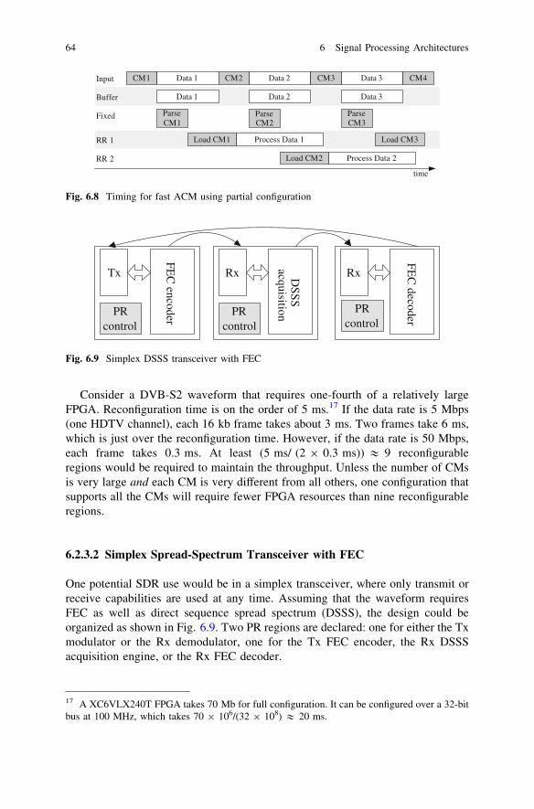
Consider a DVB-S2 waveform that requires one-fourth of a relatively largeFPGA. Reconfiguration time is on the order of 5 ms.17 If the data rate is 5 Mbps(one HDTV channel), each 16 kb frame takes about 3 ms. Two frames take 6 ms,which is just over the reconfiguration time. However, if the data rate is 50 Mbps,each frame takes 0.3 ms. At least (5 ms/ (2 9 0.3 ms)) & 9 reconfigurableregions would be required to maintain the throughput. Unless the number of CMsis very large and each CM is very different from all others, one configuration thatsupports all the CMs will require fewer FPGA resources than nine reconfigurableregions.
6.2.3.2 Simplex Spread-Spectrum Transceiver with FEC
One potential SDR use would be in a simplex transceiver, where only transmit orreceive capabilities are used at any time. Assuming that the waveform requiresFEC as well as direct sequence spread spectrum (DSSS), the design could beorganized as shown in Fig. 6.9. Two PR regions are declared: one for either the Txmodulator or the Rx demodulator, one for the Tx FEC encoder, the Rx DSSSacquisition engine, or the Rx FEC decoder.
Rx DSSS
acquisition
Tx
PR control
FEC
encoder
Rx
FEC
decoder
PR control
PR control
Fig. 6.9 Simplex DSSS transceiver with FEC
CM1 Data 1Input
Buffer
RR 1 Load CM1 Process Data 1
RR 2
CM2 Data 2 CM3 Data 3 CM4
Data 1 Data 2 Data 3
Fixed Parse CM1
Parse CM2
Parse CM3
Load CM3
Load CM2 Process Data 2
time
Fig. 6.8 Timing for fast ACM using partial configuration
17 A XC6VLX240T FPGA takes 70 Mb for full configuration. It can be configured over a 32-bitbus at 100 MHz, which takes 70 9 106/(32 9 108) & 20 ms.
64 6 Signal Processing Architectures

The SDR starts in transmit mode, then switches to receive mode, and then backto transmit. DSSS acquisition block typically requires a lot of resources but is notused after the spreading code is found. Once the spreading code has been acquired,those resources can be reconfigured as the FEC decoder while the Rx demodulatorcontinues to track the received signal.
6.2.3.3 Cognitive Radio
Another example for the use of PR in SDR applications comes in the field ofcognitive radio (CR, see Sect. 3.4). A CR receiver must scan the available spec-trum, locate energy peaks, create a channel that attempts to match the spectralshape, perform modulation recognition, and then try to demodulate. Because thespectrum must always (or at least very often) be monitored, the FFT module is leftas static, but use of the modulation recognition and demodulator are mutuallyexclusive, providing an opportunity to take advantage of PR. It is expected thatswitching between modulation recognition and demodulation will occur often asthe receiver searches the available signals for the correct one. If reconfigurationcould be achieved quickly enough, the FFT module could potentially be madereconfigurable as well. Partitioning for this CR receiver example can be seen inFig. 6.10.
6.2.3.4 Hardware Acceleration
PR can be effectively applied to hardware acceleration (see Sect. 6.6). Hardwareacceleration (HA) is used when some functions (e.g. DSSS acquisition, dispreading,and FEC decoding) in a GPP-based SDR cannot be executed in real time. Thesefunctions can then be offloaded to an FPGA-based accelerator.
If some latency is acceptable and enough memory is available, it is possible toimplement a multi-channel receiver in software while buffering data and time-
PR control
Channelizer
FFT
ModulationRecognition
PR control
Channelizer
FFT
Demodulator
Fig. 6.10 Cognitive radioreceiver
6.2 FPGA-based SDR 65

sharing the FPGA as necessary to process the data when necessary. Using anembedded microprocessor and a memory manager, portions of the FPGA could bepartially reconfigured (similar to a context switch) to process one channel’s dataand then reconfigured to process another channel’s data. Because the data can bebuffered during the reconfiguration, the only limitation is the average throughputof the FPGA. Fig. 6.11 shows a block diagram of such a system.
6.2.3.5 Partial Reconfiguration in the Virtex-4
It is important to be aware of the performance and limitations of PR implemented onthe target device. Because of the widespread use of Xilinx’s FPGAs, the Virtex-4family was chosen as the example FPGA.18 The FPGA is configured by writing bitsto its configuration memory. The configuration data is organized into frames thattarget specific areas of the FPGA through frame addresses. When using PR, thepartial bitstreams contain configuration data for a whole frame if any portion of thatframe is to be reconfigured.
Reconfiguration time is highly dependent upon the size and organization of thePR region(s). Four methods of configuring a Xilinx FPGA are listed in Table 6.1.
Estimated sizes and corresponding configuration times for a few commonblocks are given in Table 6.2. Note that approximately 10 % overhead is incurredin setting up the addressing for PR. These values assume PR region resource
Table 6.1 Partial Reconfiguration Interfaces
Port Bus width Max frequency (MHz) ls/Framea
External serial port 1 bit 100 13External serial JTAG port 1 bit 66 20External parallel SelectMap 8 bits 100 1.6Internal access port (ICAP) 32 bits 100 0.4a Configuration of one frame requires 41 32-bit words of configuration data
PR control
Memory manager
Fast
External
Memory
Function 1
SDR
using a
GPP
Function 2
Function 3
Fig. 6.11 Hardwareacceleration of software-defined radio
18 PR has not changed significantly in the Virtex-6 and -7 devices.
66 6 Signal Processing Architectures
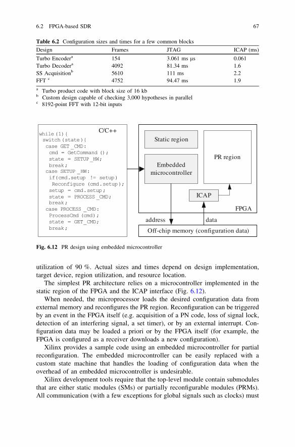
utilization of 90 %. Actual sizes and times depend on design implementation,target device, region utilization, and resource location.
The simplest PR architecture relies on a microcontroller implemented in thestatic region of the FPGA and the ICAP interface (Fig. 6.12).
When needed, the microprocessor loads the desired configuration data fromexternal memory and reconfigures the PR region. Reconfiguration can be triggeredby an event in the FPGA itself (e.g. acquisition of a PN code, loss of signal lock,detection of an interfering signal, a set timer), or by an external interrupt. Con-figuration data may be loaded a priori or by the FPGA itself (for example, theFPGA is configured as a receiver downloads a new configuration).
Xilinx provides a sample code using an embedded microcontroller for partialreconfiguration. The embedded microcontroller can be easily replaced with acustom state machine that handles the loading of configuration data when theoverhead of an embedded microcontroller is undesirable.
Xilinx development tools require that the top-level module contain submodulesthat are either static modules (SMs) or partially reconfigurable modules (PRMs).All communication (with a few exceptions for global signals such as clocks) must
Table 6.2 Configuration sizes and times for a few common blocks
Design Frames JTAG ICAP (ms)
Turbo Encodera 154 3.061 ms ls 0.061Turbo Decodera 4092 81.34 ms 1.6SS Acquisitionb 5610 111 ms 2.2FFT c 4752 94.47 ms 1.9a Turbo product code with block size of 16 kbb Custom design capable of checking 3,000 hypotheses in parallelc 8192-point FFT with 12-bit inputs
Off-chip memory (configuration data)
PR region
Static region
FPGA
ICAP
Embedded microcontroller
dataaddress
Fig. 6.12 PR design using embedded microcontroller
6.2 FPGA-based SDR 67

be explicitly declared using partition pins. An example design with two PRMs isshown in Fig. 6.13.
The required hierarchy adds a significant amount of effort when converting anexisting static design into one that is ready for PR. Having all the PRMs at the toplevel will often require routing many signals to and from another module deepwithin the main static module. For example, a modem with FEC cores embeddeddeep within both transmit and receive portions of the design requires routing allthe necessary signals up and down through the entire hierarchy in order to havepartially reconfigurable FEC modules (Fig. 6.14).
6.2.3.6 Wires on Demand
The partial reconfiguration flow described above requires static allocation of thereconfigurable areas. Signal routing between reconfigurable areas and static areasis fixed. This approach works well as long as only a few combinations of PRdesigns are required. However, it does not allow easy runtime construction offlowgraphs from a large library of relatively small blocks. An interesting effortfrom Virginia Tech is aimed at improving on the tools provided by Xilinx. The‘wires-on-demand’ concept is based on a single large PR area. The tool is then ableto automatically place and interconnect an arbitrary number of blocks within thePR area. An example of this approach applied to SDR is described in [75].The need for wires-on-demand is a reflection of relatively poor support for PRfrom Xilinx. When and if PR becomes mainstream, Xilinx will likely provide amore robust toolset that will make wires-on-demand obsolete.
6.3 Host Interface
Most SDRs can be logically separated into a block that implements a waveformand a block that decides which waveform to use. For this section, the ‘decider’ isknown as the host, while the signal processing is done by the device. Note that thehost and the device may very well be on the same chip. The host is usually a GPP,while the device can be either a GPP or hardware based (FPGA, ASIC).
In the simplest scenario, the host loads (for an FPGA-based SDR) or executes(for a GPP-based SDR) the desired waveform. If the waveform has no additional
Static Module
PRM
A
PRM
B
Top Module
partition pins
Fig. 6.13 Example designshowing two PR regions
68 6 Signal Processing Architectures

parameters that must be set, the host is done. But in many cases the loadedconfiguration (executable) can support multiple varieties of a given waveform. Forexample, the data rate may be a runtime selectable parameter. Some configurations(e.g. those in Sect. 6.2.1) can have hundreds of run-time parameters. The logicalinterface between the host and device should be carefully considered.19
Interface to a GPP-based device is dictated by the SDR software infrastructure(e.g. SCA, GNU Radio, etc.). The logical interface to a hardware-based device isfrequently up to the designer.
6.3.1 Memory-Mapped Interface to Hardware
The simplest logical interface paradigm for a hardware device is memory-mappedaccess. Each configurable parameter is given a unique address. A physical orlogical bus is established between the host and the device. The bus consists of fiverequired and two optional signals:
1. Address2. Read_Enable3. Read_Data4. Write_Enable5. Write_Data
SDR top level
Host I/FTransceiver
Transmitter Receiver
Sample-rateFECSample-rateFEC
SDR top level
Host I/FTransceiver
Transmitter Receiver
Sample-rateSample-rate
FEC
(a)
FECReconfig controller
(b)
Fig. 6.14 Hierarchical firmware view of transceiver with FEC. a Static design. b Reconfigurable
19 The author has reworked the logical interface for one complex FPGA-based SDR three timesin 6 years to support growth and maintainability..
6.3 Host Interface 69

6. [Optional] Read_ready7. [Optional] Write_acknowledge
The bus is broadcast to all the blocks in the device. Each configurableparameter is compared to the address and a parameter is set if the address matches.For example, the host would execute.WriteRegister(A_SET_DATARATE, DATARATE_1Mbps)To cause the device to set the data rate to 1 Mbps. Reasonable software design
practice dictates that the addresses and (usually) data are given descriptive names.This interface is familiar to all hardware designers. Despite its simplicity amemory-mapped interface raises a number of design issues. Address assignmenthas to be carefully considered. Multiple developers working on different blocksmust be able to get unique addresses for their blocks. Ideally, a centralized web-based tool is available to request and register each address. The tool is thenresponsible for generating source code with a mapping from address name toaddress value for each programming language used by the team (e.g. a VHDLpackage, a C header). The tool is also responsible for generating documentationwith a list of registers and their function. In the simplest designs, the address is aset of sequential integers, starting from zero. However, that approach very quicklybecomes impractical.
Consider a case where two independent development efforts are merged into asingle design. For example, a SDR is merged with a channel emulator. Each teamhas its own address mapping, and the address values between the two designs arelikely to be duplicated. One option is to renumber all the addresses. Unfortunately,this immediately obsoletes all printed documentation.20 Now consider a casewhere multiple copies of the same design are instantiated to implement a multi-channel SDR. The addresses for all the channels are now the same and it isimpossible to configure each channel for a different waveform. One solution is toassign new addresses to every instance of the design, but it makes the host soft-ware difficult to read and maintain. Instead, a hierarchical address structure shouldbe adapted. At the lowest level of hierarchy, the addresses are sequential integers.The next level of hierarchy defines the instance number (channel). The next levelof hierarchy defines the top level design (e.g. SDR, channel emulator, videoprocessor). The address should be treated as a structure with different fields. For ahardware implementation, each field would be assigned a specific number of bits.For example, if the system is expected to have no more than four different designsand each design has no more than 16 channels, D = 2, C = 4 (Fig. 6.15).
This addressing scheme works well as long as the host accesses only oneregister at a time. There are (infrequent) cases where the host may need to con-figure a register in multiple channels or even designs simultaneously. For example,a command to start processing data may be issued to the receiver and an
20 Hardware developers have an uncanny ability to remember four-digit hex values correspond-ing to addresses in the blocks they have designed and get very frustrated trying to set a registerthat has been renumbered..
70 6 Signal Processing Architectures

acquisition engine at the same time. One solution is to create a register in a level ofhierarchy above both designs that would be written to and would in turn trigger thedesigns. However, the two designs may not be even co-located. A set of broadcastaddresses can be defined (but used sparingly). One approach is to designate valueof zero to mean broadcast in each level of hierarchy. A conceptual view of thisaddressing scheme is shown in Fig. 6.16. The address is represented by a tuple{device:D, channel:C, register:R} in Fig. 6.16. Note that the hierarchy is entirelylogical and can be interpreted either as a tuple or as single value.
If interpreted as a tuple, each level of hierarchy checks the address and passesthe memory map bus down21 to the lower level of hierarchy if the address matchesthe mask. Looking at Channel 2 in SDR, we see that SDR level of hierarchy willpass addresses that have either 0 or 1 for the device field. 1 corresponds to SDR,while 0 is the broadcast identifier. Channel 2 level will pass addresses that have thechannel field set to either 0 or 2. 2 corresponds to the channel number, while 0 isthe broadcast identifier. Blocks at the lowest level of hierarchy only check if theregister field matches the value(s) assigned to that block. If interpreted as a singlevalue, the value itself is formed by an appropriate macro that combines the fields.The second approach is less elegant, but is more compatible with a hardwareinterface standard known as MHAL (see Sect. 7.1.3).
The reader has, no doubt, noticed that the hierarchical addressing schemedescribed above is very similar to the IP addressing scheme used to route packetsover the Internet. Indeed, IPv6 addressing can be used for large and software-
register #channeldesign
AGC
Track
FEC
channel=1
SDR [design = 1]
Fading
Noise
channel=1 channel=2
Channel Emulator [design = 2]
Device
(a)
(b)
D bits C bits R bits
channel=2 channel=3
register=0
register=1
register=2
AGC
Track
FEC
register=0
register=1
register=2
AGC
Track
FEC
register=0
register=1
register=2
register= 0
register=1
Fading
Noise
register=0
register =1
Fig. 6.15 Hierarchical memory-mapped addressing. a Address partitioning. b Hardware view
21 In hardware, the read and write signals can be gated (logically AND’ed with) by the mask. Insoftware, the lower level functions are simply not called.
6.3 Host Interface 71

centric SDR designs. An immediate advantage of using IP is the ability to easilysplit SDR among multiple boards.22
6.3.1.1 Acknowledge Signals
The read ready signal is not part of the classical memory map interface.23 How-ever, it is quite useful for two reasons:
1. It makes detecting software and hardware bugs related to addressing mucheasier. For example, if no unit responds to a particular read request, the hostneeds to know that the read failed. A classical memory map interface wouldreturn a random value. Likewise, if more than one unit responds to a readrequests, the addresses must have been misassigned and an error should begenerated.
2. It allows different units to take a different amount of time to respond to a readrequest. For example, some units can respond immediately, while others need afew clock cycles. Once the data are ready, the unit asserts read ready.
A write acknowledge signal is also useful in detecting misassigned addresses.
AGCx:x:1
Trackingx:x:2
Channel 1
SDR
Channel 1
Channel Emulator
Device
Trackingx:x:3
x:1:x
x:0:x
1:x:x
0:x:x
AGCx:x:1
Trackingx:x:2
Channel 2
Trackingx:x:3
x:2:x
x:0:x
AGCx:x:1
Trackingx:x:2
Channel 3
Trackingx:x:3
x:3:x
x:0:x
2:x:x0:x:x
Fadingx:x:1
Noisex:x:2
Channel 1
Fadingx:x:1
Noisex:x:2
x:1:x
x:0:x
x:2:x
x:0:x
Fig. 6.16 Representative addressing scheme with hierarchy and broadcast
22 This discussion covers only the control plane. The data plane is addressed in Sect. 7.4.23 It is part of all modern bus interfaces such as PCI or DDR3.
72 6 Signal Processing Architectures

6.3.2 Packet Interface
The memory map interface can be extended to support multiple data values (aburst) for each read/write command. In fact, most modern memory interfacessupport burst read/write operations to increase throughput. A burst read/write canbe thought of as a packet, with the first element interpreted as the address and therest of the elements treated as data. It is trivial to convert from a packet interface toa classical memory map interface by simply holding the address and read/writeline constant for the duration of the packet.
The MHAL API [76] defined for JTRS radios (see Sect. 7.1.3) uses the packetparadigm (Fig. 6.17). The address is referred to as the ‘logical destination’. Notethat, MHAL provides no guidance as to how the logical destination is to be used.It can be used to implement either a flat or hierarchical address space.
6.4 Architecture for FPGA-Based SDR
6.4.1 Configuration
The highly parallel architecture of FPGAs is ideally suited for dataflow processing,but is not well suited for control-intensive processing. Each of the reconfigurationapproaches described above requires a controller to select the desired waveform.The controller may write to registers, load a complete or partial configuration file,or perform some combination of these operations. The controller is almost alwaysimplemented in software running on a GPP. This combination of a GPP and one ormore FPGAs raises interesting computer architecture questions. FPGA devicesavailable in 2011 suggest three options:
IU Logical destination (15 bits)
Length
Payload
Least significant bit
Most significant bit
Fig. 6.17 Standard messagestructure for MHALcommunication
6.3 Host Interface 73

1. A dedicated GPP device is used alongside FPGA(s). Any GPP can be selectedfrom the very wide range of available choices. The GPP has relatively modestrequirements since it does no signal processing. An appropriate device belongsto the class of microcontrollers rather than microprocessors. The same GPP canalso be used for user interface (if any). The memory access bandwidthrequirement depends on the configuration approach:
a. High-bandwidth access to memory is needed if partial reconfiguration isused and the waveforms must be changed quickly. Some of the lower endmicrocontrollers would not be suitable. As discussed above, the GPP mustread the partial configuration file and write the data to the FPGA. There aretwo basic options for storing the configuration data: NVRAM (e.g. FLASH)and SDRAM.24 NVRAM typically shares the memory bus with the FPGA,while SDRAM is on a separate bus. NVRAM data throughput is much lowerthan for SDRAM. These two considerations motivate the use of SDRAM forpartial reconfiguration applications.
b. FPGA vendors have recognized the need for fast and simple configurationand FPGA-friendly FLASH memory is available [77,78]. These devicesallow the GPP to control and initiate the configuration without having totransfer the data itself. This way even a low-end microcontroller can achievefast reconfiguration. This approach only works for full reconfiguration.
c. Memory access is not a concern for multi-waveform configurations sinceonly a few registers have to be set to change a waveform.
2. A full-featured microcontroller can be embedded in the FPGA by using theavailable logic resources.25 This architecture raises a ‘chicken vs. egg’dilemma––the microcontroller does not exist until the FPGA is programmed, andtherefore cannot program the FPGA. An external configuration source is requiredto load the initial configuration. The embedded microcontroller can then performwaveform selection for the multi-waveform and partial reconfiguration modes.The embedded microcontroller, combined with option (1b) above, can also selecta waveform in the full reconfiguration mode.
3. An FPGA and a dedicated GPP can be combined on a single device (e.g. ZYNQfrom Xilinx [62]). Unlike an embedded microcontroller, the on-chip micro-controller is active upon power-up and does not require the FPGA to be pro-gramed. Other than single-chip integration, the design considerations are thesame as in (1).
24 Data are loaded into SDRAM prior to reconfiguration. It may be loaded from nonvolatilestorage (disk, FLASH, etc.), or received over the air.25 A hard macro microcontroller may also be available on some FPGAs (e.g. PowerPC on XilinxVirtex 2 and Virtex 4 FX series).
74 6 Signal Processing Architectures

6.4.2 Data Flow
The data flow architecture is probably the most critical decision in the FPGA-based SDR development. The two major options are:
1. Datapath with flow control2. Bus-centric
Datapath architecture is the simplest and most obvious choice. Signal pro-cessing blocks are connected in a contiguous flowgraph, closely mirroring thesystem-level block diagram. A block operates on the incoming samples one ormore at a time and passes the output to the next block in the flowgraph. Forexample, in a receiver the A/D data block passes samples to the DC-offset can-celing block, which, in turns, passes data to a frequency offset compensation block,etc.…
The simplest implementation uses one-way handshaking––either pull (Fig. 6.18b)or push (Fig. 6.18a). In a one-way push handshaking, an upstream block indicatesthat data are ready to a downstream block. The downstream block must be able toaccept and process the data. Likewise, for one-way pull handshaking a downstreamblock requests data from the upstream block. The upstream block must be able tosupply data as soon as it is requested. One-way push handshaking can be used quitesuccessfully for relatively simple receivers, while pull handshaking can be used fortransmitters.
One-way handshaking fails if one or more of the blocks cannot process data assoon as it comes in, even though it can process the average throughput.26 Theoffending block must buffer bursts of data to avoid losing it. The buffer (a FIFO) mustbe large enough to hold the longest expected burst. DSP blocks designed for SDR aremeant to be flexible and work with a wide range of waveforms. The maximum burstsize may, therefore, be unknown, or very large. It is inefficient (and inelegant) torequire these ‘handshaking’ buffers to be sprinkled throughout the design. Classicaltwo-way handshaking overcomes this problem. In two-way handshaking, anupstream block tells the downstream block that data are ready while a downstreamblock requests the data from an upstream block. Data are only transferred if bothready and request are true (Fig. 6.18c). Buffering may still be required whenusing two-way handshaking––one at the source and one at the sink.
Datapath architecture works well for high-speed designs where each block isoperating close to its maximum throughput. However, the architecture makes itawkward to share blocks among multiple data streams.
Consider a receiver supporting two data channels at 1 and 2 Mbps. The first fewblocks process A/D samples for both data streams. However, after the channelizerthe two streams are separated. Assuming that all the blocks are capable of pro-cessing 3 Mbps on average, blocks after the channelizer should be shared.
26 Clearly, if the block cannot handle even the average throughput the system will not work.
6.4 Architecture for FPGA-based SDR 75

The simple ready/request flow control cannot be applied anymore.27 Fur-thermore, blocks that retain internal state from sample to sample (e.g. filters) mustbe designed to store states for both channels and automatically switch betweenthem.28
The fixed flowgraph also limits flexibility. Consider the example above, withdifferent waveforms used for 1 Mbps and 2 Mbps channels. For one channel, thefrequency tracking block should come before the matched filter, while for thesecond channel it should come after the matched filter.29 The control and routinglogic to switch the position of a block in a flowgraph is quite messy.
Datapath architecture works well for streaming waveforms (i.e. symbols aretransmitted continuously). However, it is quite inconvenient for packet-basedwaveforms. For a packet-based waveform, the transmitter can send out a (rela-tively) short message and the receiver must be able to demodulate short messages.The problem with a datapath architecture is data in the pipeline. Consider a simpleFIR filter used for pulse shaping. The filter has some memory (4–8 symbols istypical), meaning that the last few symbols of a message are still inside the filterafter the last symbol of the message has been input to the filter (Fig. 6.19). Thefilter memory translates into a small latency for streaming data. After the messageis done, the ‘stuck’ symbols get pushed out by the next message. However,if messages are not contiguous, the stuck symbols do not get transmitted until thenext message is sent. The problem can be overcome by intentionally inserting somepadding zero symbols after each message. Of course, this requires the datapath tobe aware of the message boundaries and whether there is a gap between messages.
U D
data
ready U D
data
request
(a) (b)
U D
data
request
(c)
ready
Fig. 6.18 Handshaking. a One-way push. b One-way pull. c Two-way
Input samples Output samples
Filter
Samples stuck inside the filter
Initial transient (junk)
Fig. 6.19 Symbols ‘stuck’inside a filter (filter span is 4symbols)
27 It is quite possible to design a module to switch the flow control logic between the twochannels, but based on the author’s experience the code quickly becomes unreadable..28 This is also quite possible, but leads to lower performance, and requires significantly moredevelopment effort.29 This somewhat artificial example may be motivated by different expected frequency dynamicsfor the two channels.
76 6 Signal Processing Architectures

A bus-centric architecture replaces point-to-point connections between blockswith a shared bus. This architecture is also known as processor-centric or system-on-a-chip. Each of the DSP blocks is treated as a peripheral to a central processingunit. The CPU can be implemented on a low-end embedded GPP or even adedicated state machine. A simple example is shown in Fig. 6.20. A block ofreceived samples is buffered in memory (Fig. 6.20:1). The CPU then transfers theblock of samples to the first DSP block (Fig. 6.20:2). The output of the DSP blockis again buffered in memory.30 The internal state of the DSP block may also besaved to memory to allow seamless processing of multiple data streams (shadedblock in Fig. 6.20). Once the entire block has been processed, the CPU transfersthe output block to the second DSP block (Fig. 6.20:4). The process continuesuntil all the processing has been applied to the data.
A major problem with the architecture and dataflow described above is verylow performance and throughput. Indeed, all but one of the blocks are idle at anygiven time. The operation is very similar to executing serial (not multi-threaded)software. Although it makes poor use of FPGA resources, this architecture works ifhigh-throughput is not required.31
The key to an efficient bus-centric architecture is to offload the actual move-ment of data between blocks from the CPU to a sophisticated DMA engine.A detailed discussion of DMA engine and bus architectures is beyond the scope ofthis book. The CPU is only responsible for keeping track of available memorybuffers and scheduling data transfers. Actual transfers are handled by the DMAengine. A multi-channel DMA engine can simultaneously handle transfers to andfrom multiple blocks. Extending the example in Fig. 6.20: While block #1 isprocessing the first block of data from the source (Fig. 6.21:A), the source issaving data into a new buffer (Fig. 6.21:B). While block #2 is processing theoutput of block #1 (Fig. 6.21:C), block #1 is processing data from Fig. 6.21:B.
SourceDSP
block #1DSP
block #2DSP
block #N
Bus
CPUMemory
1
2
3
4
Sink
Fig. 6.20 Basic bus-centric architecture
30 In-place operations overwrite the input memory. Alternatively, the output is placed in adifferent part of memory.31 An FPGA is not the best device to implement a SDR with low-throughput requirements and aGPP or a DSP may be more appropriate.
6.4 Architecture for FPGA-based SDR 77

All the blocks are fully utilized in the pipelined bus-centric architecture,assuming two constraints are met:
1. Bus throughput is sufficient to sustain all the simultaneous data transfers. Forexample, a system with 10 blocks and a nominal sample rate of 5 MSPS musthave a bus capable of sustained throughput of 2 9 10 9 5 = 100 MSPS. Theconventional shared bus topology shown in Fig. 6.20 does not scale with thenumber of blocks and can quickly become a bottleneck. Memory throughput isalso a potential limiting factor, since it has the same requirements as the busthroughput.
2. All of the blocks process data at the same rate. It is easy to see that the overallthroughput is determined by the throughput of the slowest block. Fortunately,the bus-centric architecture allows makes it easy to replicate slow blocks toachieve higher throughput.
6.4.3 Advanced Bus Architectures
At least three different bus topologies can be applied to alleviate the bus andmemory throughput constraint identified above. However, before considering thealternatives let us consider when the constraint becomes an issue. The physicallayer of a typical radio consists of 15–30 discrete DSP blocks. Assume each blockprocesses complex baseband32 data sampled at X MHz with 16 bit precision. Busthroughput, B, is then
30 blocks � 2 samples/complex pair � X MHz � 2 read/write ¼ 240X MBps
A modern FPGA can support a 256 bit data bus operating at 200 MHz, giving athroughput of 6.6 GBps. Assuming, for simplicity, 100 % bus utilization, that buscan support X = 6.6 GBps/240 MBps * 25 MHz. A complex sample rate of25 MHz supports signal bandwidth up to 10–20 MHz. This bandwidth covers most
SourceDSP
block #1DSP
block #2DSP
block #N
Bus
CPU Memory
A C
Sink
B D
Fig. 6.21 Pipelined bus-centric architecture. Dashed lines indicate data flow for even numberedblock periods, while solid lines are for odd numbered
32 Complex baseband sample-rate data dominates overall throughput.
78 6 Signal Processing Architectures

of the commercial standards in use today and may be sufficient for a wide range ofSDR applications. However, a higher performance bus is required for widebandradios (e.g. 100 MHz bandwidth). A higher performance bus is best served by adistributed memory architecture. Instead of centralizing memory and DMA, eachblock has its own.
1. If the dataflow is expected to be mostly between successive blocks, a ringtopology is appropriate (Fig. 6.22a). Note that, this architecture looks quitesimilar to a datapath and therefore suffers from the same problems. In partic-ular, changing the order of blocks is no longer simple.
2. The most flexible solution is a full or partial mesh (Fig. 6.22b). The CPU is stillresponsible for configuring the DMA engines in each block, but all data transferis now point-to-point. The main disadvantage is that the number of connectionsgrows as a factorial of the number of blocks. Routing all these connectionsbecomes impractical for even a few blocks. A partial mesh prunes many of theconnections, making the hardware simpler at the cost of potentially reducedflexibility.
The reader may wonder why the FPGA fabric itself cannot be reconfigured toimplement just the desired connectivity. After all, an FPGA is essentially a sea oflogic gates with programmable interconnections. Unfortunately, the programmableinterconnection is mostly local, used to connect adjacent logic gates. A majorchange in routing (e.g. exchanging the location of two blocks) requires a newplacement of the logic gates.
A discussion of bus architectures would be incomplete without mentioning the‘network-on-a-chip’ approach (see Sect. 5.4.1 for an example). The mesh archi-tecture can be implemented by routing each bus to a port of a switch. Thisarchitecture does not scale well because the switch quickly becomes too large.Alternatively, a hierarchical mesh structure can be formed by grouping blocks that
DSP block #1
Memory
DMA
CPU
DSP block #2
Memory
DMA
DSP block #3
Memory
DMA
DSP block #1
Memory
DMA
DSP block #2
Memory
DMA
DSP block #3
Memory
DMA
CPU
(a) (b)
Fig. 6.22 Higher performance bus architectures. a Ring. b Full mesh
6.4 Architecture for FPGA-based SDR 79

may conceivably need to transfer data to each other. Extending the concept of abus to that of a fully switched network also facilitates multi-device and multi-board solutions for very large SDRs.
6.4.4 Parallelizing for Higher Throughput
The slowest block in the signal processing chain sets the maximum throughput.The classical solution to increasing throughput is parallelization. A block may beparallelized internally, thereby appearing faster, or multiple blocks can beinstantiated. The first approach does not depend on the dataflow architecture. Thesecond approach requires the CPU to appropriately schedule each of the replicatedblocks. Neither approach is preferred over the other because the implementationburden is simply shifted. However, if the block in question is a black box (or alicensed core that cannot be modified), only replication is an option. Four classesof blocks must be considered, with different approaches to parallelization for each:
1. Memoryless blocks process data one sample at a time and possess no internalstate. Examples include: upconverter, fixed DC offset canceler. These blocksare simply replicated.
2. Some blocks process a fixed set of samples at a time and then reset to the initialstate. Examples include: block FEC codes (Reed-Solomon, Turbo, LDPC),terminated convolutional codes, block interleavers, fast Fourier transforms.These blocks are simply replicated and the CPU makes sure that one or morecomplete sets are processed at once.
3. Finite memory blocks process data one sample at a time, but possess an internalstate. The output depends on the current and some of the past input. Examplesinclude: FIR filters, resamplers. These blocks are more difficult to parallelizebecause the internal state becomes invalid for discontinuous input. One solutionis to overlap data processed by each instance of the block. The overlap, N, mustbe long enough to account for the internal state. The first N outputs from eachinstance are then discarded. As long as N is small relative to the number ofsamples in a chunk, the overhead is negligible
4. Blocks with infinite memory have internal feedback. The output depends on allof the past input. Examples include: IIR filters, phase and symbol trackingloops, automatic gain control loops. These blocks are by far the hardest toparallelize and must be considered on a case-by-case basis. If at all possible,these blocks should be parallelized internally to hide the complexity from theCPU. For example, look-ahead computation can be used to speedup IIR filters(see Chap. 10 in [79]). Feedback loops for tracking and adaptation may beparallelized if the loop bandwidth is small relative to the duration of the chunkof samples processed at once.
The technique of parallelization is obviously not specific to the design of SDR.However, it does come up a lot since the same SDR hardware platform may be
80 6 Signal Processing Architectures
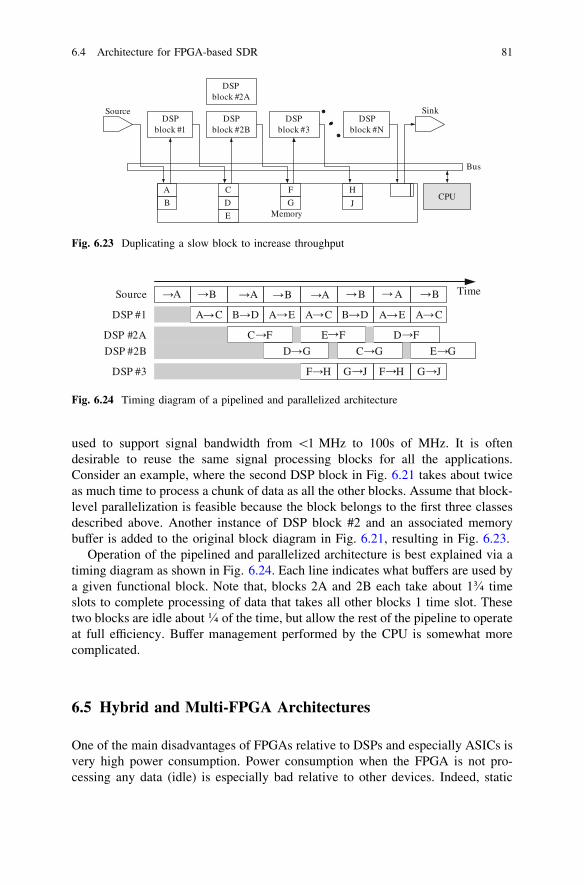
used to support signal bandwidth from \1 MHz to 100s of MHz. It is oftendesirable to reuse the same signal processing blocks for all the applications.Consider an example, where the second DSP block in Fig. 6.21 takes about twiceas much time to process a chunk of data as all the other blocks. Assume that block-level parallelization is feasible because the block belongs to the first three classesdescribed above. Another instance of DSP block #2 and an associated memorybuffer is added to the original block diagram in Fig. 6.21, resulting in Fig. 6.23.
Operation of the pipelined and parallelized architecture is best explained via atiming diagram as shown in Fig. 6.24. Each line indicates what buffers are used bya given functional block. Note that, blocks 2A and 2B each take about 1� timeslots to complete processing of data that takes all other blocks 1 time slot. Thesetwo blocks are idle about � of the time, but allow the rest of the pipeline to operateat full efficiency. Buffer management performed by the CPU is somewhat morecomplicated.
6.5 Hybrid and Multi-FPGA Architectures
One of the main disadvantages of FPGAs relative to DSPs and especially ASICs isvery high power consumption. Power consumption when the FPGA is not pro-cessing any data (idle) is especially bad relative to other devices. Indeed, static
SourceDSP
block #1DSP
block #2BDSP
block #N
Bus
CPU
Memory
A C
Sink
B D
DSP block #2A
E
DSP block #3
F
G
H
J
Fig. 6.23 Duplicating a slow block to increase throughput
A
A C
B A B A B A B
B D A E
C F
D G
E F
A C B D A E
C G
D F
A C
E G
F H G J F H G J
Time
DSP #2A
DSP #2B
DSP #3
DSP #1
Source
Fig. 6.24 Timing diagram of a pipelined and parallelized architecture
6.4 Architecture for FPGA-based SDR 81

power consumption due to leakage can easily account for over half of the totalpower [80]. Not surprisingly, static power consumption for the high end, high-performance FPGAs is worse than for the lower end versions. FPGA vendors arewell aware of this problem and are actively working to address it [80, 81].However, for the foreseeable future, high-end FPGAs will continue to draw a lot ofpower when idle. Power consumption motivates a multi-FPGA or a hybrid FPGA/DSP architecture.
Consider a SDR that supports a wide range of waveforms, including some thatare spread. As mentioned previously, DSSS acquisition and FEC decoding aretypically the most computationally intensive blocks in a SDR. This particular radiois used for relatively low rate communications (\1 Mbps). All of the signal pro-cessing, except for DSSS acquisition, can be easily implemented on a low-powerFPGA such as Spartan/Artix/Cyclone or a DSP. Acquisition alone requires10 9 more computational resources than the rest of the radio. This is not at allunreasonable if the spreading gain (see Sect. A.4.8) is large and the spreading codeis either nonrepeating or has a long period. The floorplan for a single-FPGAsolution would look like Fig. 6.25a.
The code offset for a streaming (vs. packet-based) DSSS waveform33 has to beacquired once at the beginning of communication and is then tracked by the
DSSSAcquisition
DSSSAcquisition
Virtex-class FPGA
Artix-class FPGA
Virtex-class FPGA
(a) (b)
powerpower
Despreading
Sample-rateprocessing
Symbol-rate processing & FEC
Con
trol
ler
Despreading
Sample-rateprocessing
Symbol-rate processing & FEC
Con
trol
ler
Fig. 6.25 Implementing a SDR with DSSS support on an FPGA. a One device b Low power
33 GPS is a classical example of a streaming DSSS waveform. WiFi 802.11a is a classicalexample of a packet-based DSSS waveform.
82 6 Signal Processing Architectures

symbol-rate processing in the receiver. Thus, the acquisition engine is idle most ofthe time while SDR is receiving a streaming DSSS waveform. However, thetransistors dedicated to implementing the engine continue to draw standby power.Assuming standby power is about half of the total power, the idle acquisitionengine can use 10 9 � = 5 times more power than the active part of the SDR.This is clearly unacceptable for a low-power SDR. An obvious solution is shownin Fig. 6.25b. The infrequently used block is moved to a separate FPGA, while therest of the SDR is implemented on a small and low-power FPGA (or a DSP). Thepower supply to the large FPGA is enabled34 by the controller on the small FPGAwhenever acquisition is needed, and is disabled the rest of the time. This approachis known as a ‘power island’ and is widely used on large ASICs. It is only a matterof time until FPGAs have user-controlled power islands, but until then a two-FPGA solution can result in dramatic power reduction.
An unusual radio used for a sensor in a wireless sensor net provides anotherexample. A sensor measures concentration of a particular chemical and transmitsthe results on a regular basis. Very infrequently, the sensor is scheduled to receivean update (perhaps change the chemical to monitor). A demodulator for a givenwaveform is almost always significantly more complex than the modulator.It would be quite inefficient to always have the receiver loaded in the FPGA,wasting standby power. Instead, the large FPGA is turned on and configured withthe receiver logic only when the node is scheduled to receive an update.
The general concept of using a low-power device most of the time but having alot of signal processing resources ‘in reserve’ is not unique to FPGAs. However,it is not as effective when applied to DSPs or GPPs because these devices alreadysupport power islands on-chip. Leakage power is less of a problem and powerconsumption can be scaled by changing the operating clock frequency or puttingthe device in various low-power modes.
6.6 Hardware Acceleration
A hardware-accelerated architecture follows naturally out of the bus-centric FPGAarchitecture. A GPP is the best platform for SDR development if flexibility andrapid development are more important than size, weight, and power. This is thecase for many research SDRs and for SDRs in ground stations. Unfortunately, even
34 At least three solutions should be considered for the power ‘switch’: (1) low dropout regulator(LDO), (2) dedicated DC/DC converter or a separate channel on a multi-channel DC/DC, and (3)a power FET. LDOs are generally not recommended since FPGAs do not require a particularlyclean main digital supply, making LDO unnecessary. Further, even a small voltage drop acrossthe LDO results in significant power dissipation since the current is very high. A dedicated DC/DC is a good choice if board space and cost are not major drivers. However, a low-power deviceis typically also a small device and may not have the additional space required for a DC/DC. Apower FET acts as an almost ideal switch with a resistance of about 2 mX.
6.5 Hybrid and Multi-FPGA Architectures 83

the fastest GPPs available today cannot process wideband and complex waveformsin real time. Analysis of the throughput bottleneck in a typical radio receiver on aGPP reveals one or two functional blocks that consume the bulk of computationaltime. In particular, GPPs are not well suited for two common receiver functions:DSSS acquisition and FEC decoding. These functions require many identicaloperations on low-precision data. A GPP is optimally utilized when the dataprecision is equal to the internal datapath width––usually 64 bits. Data precisionfor DSSS acquisition is typically only 2–4 bits, while soft decisions used for FECdecoding are typically less than 5 bits. FPGAs, on the other hand, excel at this typeof processing. An obvious solution is to offload a minimum35 set of operationsfrom the GPP to an FPGA that would allow the combined system to achieve real-time throughput.
The concept of HA has been around since the 1980s, when the early fixed-pointprocessors (e.g. 80386DX) used coprocessors (80387) to compute floating-pointarithmetic operations. Coprocessors have become a ubiquitous part of today’scomputers in the form of graphics processing units (i.e., graphics cards). HA doesnot always mean having a separate device—HA blocks are routinely integrated onthe same die as the GPP. For example, DSP chips from TI include multiple HAblocks to accelerate error correction decoding, while GPPs from Intel now includea HA block to accelerate cryptography. While the application of ASIC HA hasproven itself valuable over the years, the value of flexible or reconfigurable HA hasbeen uncertain. As little as one decade ago, work was done that concluded that thetechnology at that time did not provide enough gains to warrant the efforts of HA[82]. While the idea of accelerating software through the use of specializedhardware is not new, the advancement of today’s HA boards along with increasingtransfer speeds between the main processor and the acceleration hardware hasmade general HA an attractive alternative to the current software-only solutions.HA is closely related to the concept of reconfigurable computing [83].
Despite compelling performance improvement offered by HA, it remainsarchitecture of ‘last resort’. Software developers will only consider HA if thealternative is a pure FPGA-based architecture. The reluctance is understandablesince a different skill set is now required in the team to develop the HA logic.
6.6.1 Software Considerations
The goal of a HA development is to closely resemble an all-software development.The HA interface API must be designed to be transparent to the software devel-oper. Indeed, as GPP processing power scales with Moore’s law, acceleratedfunctions may be replaced with their software equivalents without requiring any
35 Even if some functions are more optimally implemented on an FPGA, they should remain onthe GPP as long as the throughput requirements are met.
84 6 Signal Processing Architectures

changes to the calling function. The decision about which functions should bemoved to HA is typically obvious––FEC decoding and DSSS acquisition are thefirst candidates. Other functions are not as clear––DSSS despreading, FFT oper-ations for OFDM are all computationally intensive but can be done quite efficientlyon a GPP. The combination of cache hits and SIMD instructions makes it difficultto estimate the performance of a given function on a modern GPP. Simplycounting the number of arithmetic operations is not sufficient. Classical softwareengineering doctrine teaches ‘‘don’t optimize unless you have to.’’ Thus, HA isapplied once an all-software SDR fails to achieve the require throughput. Opti-mization then begins by first profiling the SDR application using a standard toolsuch as Intel Vtune [84] or gprof. Profiling should identify one or a few functionsthat take up most of the computation time. Note that if computation time is evenlydistributed across many functions, the SDR application is not likely to benefit fromHA. The maximum potential performance increase is given by Amdahl’s law:
T ¼ 1ð1� aÞ þ a
s
where a is the fraction of the execution time of the original software that will beaccelerated, s is the speedup obtained for that portion of the software, and T is theoverall speedup. For example, if a single function takes half of the computationtime and that function can be accelerated to take zero time (i.e. s = ?), the overallspeedup is no more than a factor of 2.
When HA is finally embraced, a number of tradeoffs must be made:
1. Choice of hardware.
a. The first choice is always a SPU, specifically a GPGPU (see Sect. 5.4).GPGPU development flow is relatively similar to GPP development and usesthe ‘C’ or C ++ language familiar to GPP developers. Further, GPGPUboard and tool suite are relatively inexpensive.
b. FPGAs are used for HA if a GPGPU solution does not provide sufficientthroughput [85], or requires too much power, or if FPGA development skillsare available to the team.
2. Physical interface. Throughput and latency between the GPP and HA are oftenmore important than the raw processing power of the HA. Vendors attempt todifferentiate themselves by offering HA solutions for every available GPPinterface, as shown in Fig. 6.26a.
a. PCIe is the most common and widely available choice. A 16-lane PCIe 3.0board offers a theoretical bidirectional throughput of 16 GB/s. Latency isbelow 250 ns. This throughput far exceeds the computational capabilities oftoday’s processors––i.e. the GPP cannot process data fast enough to fill thelink. A representative FPGA accelerator board is available from Nallatech[86], while a representative GPGPU board is available from Nvidia [87].PCIe is suitable for the vast majority of SDR implementations with HA.
6.6 Hardware Acceleration 85

A high-end GPP motherboard provides up to four 16x PCIe slots [88], andexternal PCIe expansion solutions are available [89]. PCIe is the only optionavailable for GPU acceleration.
b. Direct access to the processor front size bus allows exotic HA boards toachieve higher throughput, and more importantly, significantly lowerlatency than the PCIe bus. Representative boards are available fromNallatech for Intel GPP [90] and from XtremeData for AMD GPP [91].36
These solutions are targeted for the scientific computing market.c. Network-attached HAs are appropriate when one or more accelerators must
be shared between many GPPs (Figure 6.26b). 10 GbE provides throughputjust under 1 GB/s and latency of just under 5 ls. Note that these metrics areboth about one order of magnitude worse than a PCIe connection.37
The effect of throughput and latency on the performance of a HA SDR is notstraightforward, but depends on the specifics of the waveform. Clearly, throughputmust be sufficient to support real-time transfer of data from the GPP to HA andback. For example:
GPP
RAM
HA (b)
Bridge
Ethernet
HA (a)
HA (c)
Front side bus
PCIe
10 GbE
HA (c) HA (c)
GPP GPP
GPP GPP
10 GbE switch
(a) (b)
Fig. 6.26 Hardware acceleration options. a Direct attach b Switch
36 This product is apparently no longer supported. The market for front-side-bus accelerators isvery limited and the benefits over PCIe accelerators are small.37 Lower end solutions using 1 GbE links are possible, but are not recommended since the price/performance of the 10 GbE links is significantly better.
86 6 Signal Processing Architectures

A SDR receiver must process a signal sampled at 1 MHz with 8 bit precision.HA is used to implement the first frequency conversion. A minimum of 8 Mbpsbidirectional throughput is required to send the raw samples to HA and get themback to the GPP. However, this throughput may be much too low in a practicalapplication, as discussed below.
The fundamental hurdle of ensuring efficient HA is guaranteeing that the timerequired to transfer the data to and from the acceleration hardware is less than thetime required to simply process the data on the GPP. Figure 6.27 shows a sim-plified example of using HA to speed up a generic Function B. The long transfertimes incurred by HA1 make the total latency longer (lower throughput thansimply using a GPP), whereas the short transfer times associated with HA2 makethe total latency shorter (higher throughput). While processing data on specializedhardware is significantly faster than on a GPP, the overhead involved in trans-ferring the data is the key metric in determining the potential performanceimprovement.
Direct Memory Access (DMA) allows the GPP to continue processing duringdata transfers. DMA is only possible if HA has direct access to the GPP memorythrough the PCIe or front side bus (Fig. 6.26a). Network-attached HA (Fig. 6.26b)requires GPP to handle the network packets38 and the subsequent discussion doesnot apply. For DMA transfers to the hardware, the GPP is required to move thedata into a special area of locked memory. The GPP can then inform that hardwarethat the data are ready and proceed to other processing. At that point, it is up to thehardware to retrieve the data directly from the memory without the involvement ofthe GPP. When the hardware has finished processing the data, it can place itdirectly back in the locked memory. The GPP can be informed that the processeddata is available through the use of interrupts. A scenario is illustrated in Fig. 6.29showing hardware acceleration of three different functions using DMA transfers.The GPP quickly sets up three DMA transfers and continues processing other data,while the hardware controller transfers the data.
FunctionC
GPPonly
HAFunc B
FunctionB
Function A
Function A
FunctionC
HAFunc B
Function A
FunctionC
HA1
HA2
time
Fig. 6.27 Conceptual idea of how data transfer latency affects the benefits of hardwareacceleration (shaded blocks denote data transfer)
38 Technically, DMA transfers are still taking place between the GPP and the network card.
6.6 Hardware Acceleration 87

A device on the bus with its own DMA engine can act as the bus master (vs.slave-only) and independently initiate data transfer to and from system memory.39
All modern GPPs have a DMA engine and are therefore bus masters. At firstglance, it appears that one DMA engine on a bus is sufficient and a HA does notneed one. In fact, the simplest HA implemented in a FPGA may forgo a DMAengine. All GPU HAs do have a full-featured DMA engine. A dedicated DMAengine on HA reduces the load on the GPP by eliminating one interrupt andconsolidating transfer setup (Fig. 6.28). Further, the GPP DMA is used for soft-ware processing, and DMA resources (channels) may not be available at all times.
After each DMA transfer completes,40 the HAs start working and interrupt theGPP when the data has been processed. The GPP can then initiate the DMA read toretrieve the data from the hardware. It is important to note that for the exampleshown in Fig. 6.29, the bus is occupied most of the time indicating that datatransfer limits overall throughput. The HA resources are idle approximately 50 %of the time due to the data transfer bottleneck.
Modern bus architectures allow simultaneous writing and reading of data.A sufficiently sophisticated DMA engine can take advantage of this feature andread output of one HA while writing data to another one.
Setup GPP HA
Transfer Data
Process Data
Setup HA GPP
Transfer Data
Setup GPP HA and
HA GPP
Transfer Data
GPP
GP
PD
MA
HA
GPP
HA
DM
AH
A
(a)
(b)
Transfer Data
Process Data
Fig. 6.28 Differences between a slave-only HA and b bus master HA (arrows indicateinterrupts)
39 Incidentally, DMA can also be used to transfer data between multiple HA boards in the samesystem.40 A large class of HA can start processing data before the DMA completes. For example, afilter.
88 6 Signal Processing Architectures

6.6.2 Multiple HA and Resource Sharing
Consider a SDR processing multiple data streams in parallel. All the streams mustshare a single HA, resulting in potential contention. The simplest case involvestwo streams requesting access to the same HA. The HA API is responsible formaintaining appropriate locks (semaphores) to provide exclusive access to sharedhardware. A supervising software layer needs to be developed to implement asharing scheme (Fig. 6.30). Such a scheme may be very simple (round-robin, first-request, random-grant, etc.) or rather complex with different priority levels foreach stream.
Another layer of complexity is introduced if multiple HA functions are pro-vided, but only a subset (e.g. one) can be available at any given time. Some time isrequired to switch among different HA functions. This time can be very short for aGPU HA, or quite long for an FPGA HA that requires loading a new configuration.The HA supervisor must now take into account not just the immediate request(s),but the entire request queue. For example, if streams 1 and 3 request HA functionA, and stream 2 requests HA function B, it is more efficient41 to service streams 1and 3 followed by 2 rather than servicing them in order and incurring tworeconfiguration delays (Fig. 6.31). FPGA-based HA introduce another degree offreedom if multiple but not all functions can be supported simultaneously in agiven configuration. For example, stream 1 requests function A, stream 2 requestsfunction B, stream 3 requests function C. Functions A and C fit into an FPGA
GPP
DMA
HA1
1 2
write datafor HA1
write data for HA2
Process Data
Process Data
read data from HA1
read data from HA2
1 23
write data for HA3
Process Data
read data from HA3
3
HA2
HA3
Set up for DMA Transmit Handle DMA Receive
IDLE
IDLE
Available for other processing
time
Fig. 6.29 Three-accelerator transfer scenario using DMA
41 Efficiency may have to be sacrificed if the processes cannot tolerate additional latency..
6.6 Hardware Acceleration 89

simultaneously, but B requires the entire FPGA.42 The supervisor should, there-fore, service streams 1 and 3 first, followed by stream 2.
Scheduling HA becomes significantly more difficult for a massively multi-channel system. A cellular basestation is a representative example, with one SDR
Receiver #1
Receiver #2
Receiver #N
GPP
Hardware Accelerator
HA AHA B
HA C
Bus
Developed in ‘C’, Matlab, X-Midas
Developed in VHDL, Verilog, Simulink
HAsupervisor
Load/ConfigInterface HW
Library ofacceleratorfunctions
Fig. 6.30 Hardware accelerated architecture detail
A()S1
B()S2
A()S3
HA LoadA
Service1
Continue …
Service3
Continue …
LoadB
Service2
Continue …
A()S1
B()S2
A()S3
HA LoadA
Service1
Continue …
Service3
Continue …
LoadB
Service2
Continue …
LoadA
(a)
(b)
Fig. 6.31 Scheduling for resource contention. a Suboptimal. b Optimal
42 A plausible scenario is: functions A and C are FEC decoders, while function B is a DSSSacquisition. B takes a lot more FPGA resources and cannot share the FPGA with any otherfunction.
90 6 Signal Processing Architectures

supporting dozens or even hundreds of users. Consider the case with only one HAfunction (e.g. turbo decoding) shared among 11 streams. Let the acceleratedprocessing time be 10 times shorter than doing the same function in software. Ifthe streams are asynchronous to each other, there will be a time when all streamsrequest the HA function at the same time. The supervisor will queue up all 11users. The 11th user will have to wait 10 9 processing time to gain access to theHA. In that case, it is better off simply executing the function in software. A robustsupervisor should detect this condition and execute the function not using HA.
Partial reconfiguration (PR, see Sect. 6.2.3) is a natural fit for FPGA-based HA.In fact, it is the only truly compelling case for the user of partial reconfigurationthat the author has come across. Modern FPGAs are large enough to simulta-neously host multiple HA functions.43 The desired mix of functions depends on thewaveform(s) the SDR is processing. For example, a cellular basestation may havea mix of 2, 3, and 4G users. 2G waveforms use a Viterbi decoder, 3G use a Turbodecoder, while 4G use an LDPC decoder. For every new user, the HA supervisorloads an appropriate function into unallocated FPGA space. Unused functions areoverwritten as needed. The key advantage of PR is that all the functions continueoperating while a new one is loaded. Existing data streams are not interrupted asnew ones are added or removed. As discussed in Sect. 6.2.3.5, partial reconfigu-ration requires the developer to define fixed-size regions with fixed interconnect tothe static part of the FPGA. These two constraints may result in suboptimal uti-lization of the FPGA resources since the region size must be large enough toaccommodate the largest HA function. Multiple smaller HA functions can beimplemented inside a given region as shown in Fig. 6.32.
Reconfig Region
DMA Engine
Reconfig Region
Reconfig Region Reconfig Region
LDPC
Tur
bo
Tur
bo
Vite
rbi
Vite
rbi
Vite
rbi
Vite
rbi
Reconfig.Engine
Unallocated (available)
Fig. 6.32 Allocatingreconfigurable regions to HAfunctions
43 For example, a Virtex-6 LX240 device can hold 30 3GPP Turbo Decoders, or 60 ViterbiDecoders, or 4 802.16e LDPC decoders.
6.6 Hardware Acceleration 91

6.7 Multi-Channel SDR
Some SDRs are designed to support many simultaneous users sharing the sameband. For example, a radio translating between incompatible radios of police andthe National Guard has to support dozens of simultaneous users and allow any userto talk to any other user. Each user may use a different waveform with a very widerange of data ranges (e.g. from 1 Kbps to 100 Mbps). Most users need a few Kbpsfor voice; others need real-time video feeds; and the command and control centercan easily require 100 Mbps for satellite up/downlink. It is difficult to predict whatmix of different user types and waveforms will be required at any time. Thissection discusses three architectures for implementing such a SDR (for concise-ness only the transmitter is discussed):
1. A bank of individual SDRs connected to a shared antenna2. Individual SDRs sharing a common RFFE and digitizer3. An integrated multi-channel radio with a shared pool of DSP resources and a
common RFFE and digitizer.
The simplest architecture for such a multi-channel SDR consists of a bank ofindividual SDRs, each supporting one or more channels as shown in Fig. 6.33.Each SDR has a dedicated RF front end and requires a dedicated link to theantenna(s). An RF combiner adds all the signals together before transmission. Thisarchitecture is used in most SDRs of this class deployed in 2011.
The advantages are:
• More radios can be quickly and easily added by simply connecting to unusedports on the combiner.
• Minimal coordination is required between vendors of different radios.• Each radio can operate independently if needed and does not rely on any
existing infrastructure.
The disadvantages are:
• Extensive cabling is required. RF cables take up space. Since each cable carriersthe output of the radio’s power amplifier, it must be able to handle the power.
Medium Rate SDR RF
Low Rate SDR RF
RF
Com
bine
r
Medium Rate SDR RF
High Rate SDR RF
M
N
Low Rate SDR RFLow Rate SDR RF
Fig. 6.33 Simple architecture for multi-channel SDR
92 6 Signal Processing Architectures
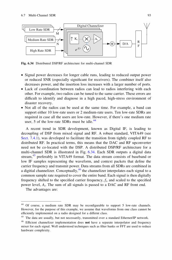
• Signal power decreases for longer cable runs, leading to reduced output poweror reduced SNR (especially significant for receivers). The combiner itself alsodecreases power, and the insertion loss increases with a larger number of ports.
• Lack of coordination between radios can lead to radios interfering with eachother. For example, two radios can be tuned to the same carrier. These errors aredifficult to identify and diagnose in a high paced, high-stress environment ofdisaster recovery.
• Not all of the radios can be used at the same time. For example, a band cansupport either 10 low-rate users or 2 medium-rate users. Ten low-rate SDRs arerequired in case all the users are low-rate. However, if there’s one medium rateuser, 5 of the low-rate SDRs must be idle.44
A recent trend in SDR development, known as Digital IF, is leading todecoupling of DSP from mixed signal and RF. A robust standard, VITA49 (seeSect. 7.4.1), was developed to facilitate the transition from tightly coupled RF todistributed RF. In practical terms, this means that the DAC and RF upconverterneed not be co-located with the DSP. A distributed DSP/RF architecture for amulti-channel SDR is illustrated in Fig. 6.34. Each SDR outputs a digital datastream,45 preferably in VITA49 format. The data stream consists of baseband orlow IF samples representing the waveform, and context packets that define thecarrier frequency and transmit power. Data streams from all SDRs are combined ina digitial channelizer. Conceptually,46 the channelizer interpolates each signal to acommon sample rate required to cover the entire band. Each signal is then digitallyfrequency shifted to the specified carrier frequency, fi, and scaled to the specifiedpower level, Ai. The sum of all signals is passed to a DAC and RF front end.
The advantages are:
Medium Rate SDR
Low Rate SDRLow Rate SDRLow Rate SDR
Medium Rate SDR
High Rate SDR
Ki
tjfie
Digital Channelizer
M
NRF
D/A
Ai
Fig. 6.34 Distributed DSP/RF architecture for multi-channel SDR
44 Of course, a medium rate SDR may be reconfigurable to support 5 low-rate channels.However, for the purpose of this example, we assume that waveforms from one class cannot beefficiently implemented on a radio designed for a differnt class.45 The data are usually, but not necessarily, transmitted over a standard Ethernet/IP network.46 Efficient channelizer implementation does not have a separate interpolator and frequencymixer for each signal. Well understood techniques such as filter banks or FFT are used to reducehardware complexity.
6.7 Multi-Channel SDR 93
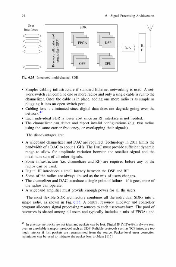
• Simpler cabling infrastructure if standard Ethernet networking is used. A net-work switch can combine one or more radios and only a single cable is run to thechannelizer. Once the cable is in place, adding one more radio is as simple asplugging it into an open switch port.
• Cabling loss is eliminated since digital data does not degrade going over thenetwork.47
• Each individual SDR is lower cost since an RF interface is not needed.• The channelizer can detect and report invalid configurations (e.g. two radios
using the same carrier frequency, or overlapping their signals).
The disadvantages are:
• A wideband channelizer and DAC are required. Technology in 2011 limits thebandwidth of a DAC to about 1 GHz. The DAC must provide sufficient dynamicrange to allow for amplitude variation between the smallest signal and themaximum sum of all other signals.
• Some infrastructure (i.e. channelizer and RF) are required before any of theradios can be used.
• Digital IF introduces a small latency between the DSP and RF.• Some of the radios are always unused as the mix of users changes.• The channelizer and DAC introduce a single point of failure—if it goes, none of
the radios can operate.• A wideband amplifier must provide enough power for all the users.
The most flexible SDR architecture combines all the individual SDRs into asingle radio, as shown in Fig. 6.35. A central resource allocator and controllerprogram allocates signal processing resources to each user/waveform. The pool ofresources is shared among all users and typically includes a mix of FPGAs and
Res
ourc
eal
loca
tor
and
cont
rolle
r(G
PP)
FPGA
DSPDSP
DSP
GPPGPP
GPP
SPUSPU
SPU
Userinterfaces
RF
D/A
SDR
Fig. 6.35 Integrated multi-channel SDR
47 In practice, networks are not ideal and packets can be lost. Digital IF (VITA49) is always sentover an unreliable transport protocol such as UDP. Reliable protocols such as TCP introduce toomuch latency if lost packets are retransmitted from the source. Packet-level error correctiontechniques can be used to mitigate the packet loss problem [115].
94 6 Signal Processing Architectures

GPPs. The controller configures FPGA bit loads and GPP software loads in realtime, as the user mix changes. The controller also configures data flow between theDSP resources and the DAC. Sharing the resources among many users allows theentire radio to use fewer resources than separate radios. Note that this architectureis a large-scale version of the one described in Sect. 6.6.2. Some of the DSPresources are likely allocated to implement a digital channelizer like the onedescribed above.
The advantages are:
• Efficient use of DSP resources. The peak usage is always smaller than the sumof all supported users since not all users can be active simultaneously. Thesavings can be quite dramatic is one user requires a large burst of resources (e.g.to acquire a highly spread, low power signal).
• Centralized control ensures that users cannot interfere with each other.• Reduced cost to develop new waveforms since the developer can leverage a lot
of existing infrastructure, both hardware, and firmware.
The disadvantages are:
• One organization must bear the cost of developing and maintaining a large andcomplex SDR. In other architectures, each organization is responsible for itsown radios.
• Development of new waveforms for new users can be complicated since theknowledge base required to work with the complex system may be limitedoutside the developer of the system.
• The resource allocator and controller is a very sophisticated piece of softwareand is therefore time-consuming and expensive to develop.
• Centralized processing introduces a single point of failure.
6.7 Multi-Channel SDR 95

Chapter 7SDR Standardization
SDR hardware has matured to the point where wide deployment is called for.However, many potential users are concerned that lack of standards makesadopting a particular hardware platform risky since software and firmwaredeveloped for that platform may not be portable to other hardware. SDR standardsmust address three different parts of a waveform life cycle:
1. Describe the waveform. A waveform description should be entirely hardwareindependent but contain all the necessary information to implement thewaveform on appropriate hardware.
2. Implement the waveform. Waveform implementation should be done in arelatively hardware-independent environment to facilitate portability to differ-ent hardware platforms.
3. Control the waveform. Once the waveform is operating, its features may bemodified at runtime.
Standardization of SDR has been progressing for many years. The JTRS/SCAstandard developed by the US Army [76] and STRS standard developed by NASA[92] define robust and powerful infrastructures for flexible radios. These standardsare described in detail in the next two sections. There is no accepted standard fordescribing the intent rather than the implementation of a waveform for SDR. Onepotential solution is described in Sect. 7.3. Finally, Sect. 7.4 covers low-levelstandards for data exchange between SDR components.
7.1 Software Communications Architecture and JTRS
The US military uses and maintains dozens of different radios. Devices built tomilitary specs last much longer than their commercial equivalents, and old devicesremain in use as new versions are procured. Further, each branch of the Army hasdifferent requirements for communications (e.g., a Delta Force operative has verydifferent needs than a tank brigade commander), and thus procures a different
E. Grayver, Implementing Software Defined Radio,DOI: 10.1007/978-1-4419-9332-8_7, � Springer Science+Business Media New York 2013
97

radio. The resulting Babel of different waveforms made the Army very interestedin SDR. The largest single SDR development effort is spearheaded by the jointtactical radio system (JTRS) joint program executive office (JPEO)1 [93]. TheJTRS program started in 1997 and was still ongoing in 2011. Its stated goal isdevelopment of a standard to facilitate reuse of waveform code between differentradio platforms.
The main standard developed by JTRS is the software communications archi-tecture (SCA). SCA defines how waveform components are defined, created,connected together, and the environment in which they operate. [94]. The standardwas developed with a very software-centric view—an SCA-compliant radio wasenvisioned as a true SDR running on a GPP. Unfortunately, at the time SCA wasdefined, GPPs were relatively slow and not up to the task of running a waveform.SCA radios were perceived as very slow, inefficient, and inelegant. In the pastdecade, GPPs have caught up with this vision and SCA implementations havebecome more efficient. Just when JTRS started fielding actual devices, the JPEOstarted an effort to update the SCA. A draft specification of SCA Next was releasedin 2010.
7.1.1 SCA Background
A complete discussion of the SCA is beyond the scope of this book, and the readeris encouraged to review [94]. The SCA defines:
• An operating system (RTOS) for the hardware that the radio runs on. The OSmust be substantially POSIX compliant, implying availability of a reasonablypowerful GPP (i.e., an 8-bit microcontroller is probably not sufficient).
• A middleware layer that takes care of connecting different parts of the radiotogether and handles data transfer between them. In the first version of SCA(2.2), the middleware layer had to be CORBA. CORBA is an industrial-gradesoftware architecture construct that was developed to facilitate communicationsbetween software written in many different languages and executing acrossmultiple computers. The SCA Next standard removes the requirement that themiddleware be CORBA and leaves it up to the radio developer. Since all SCAradios at this time rely on CORBA, it will be assumed for subsequent discussion.
• A set of interface definition language (IDL) classes provide an abstract interfaceto different objects that make up a radio (e.g., IO ports, components, devices,etc.). These classes, together with software code that enables their use, areknown as the core framework (CF).
• An XML ontology (Domain Profile) to describe all the components that make upa radio and how these components are to be interconnected and executed toimplement the desired waveform.
1 For conciseness, JTRS is used to refer both to the program and the office.
98 7 SDR Standardization

• APIs for many frequently used interfaces (e.g., audio, Ethernet, etc.)
A conceptual hierarchy of the different parts of SCA is shown in Fig. 7.1. Thefirst takeaway is that SCA is a large and complex system. It is designed to addresssecurity requirements of military radios and has built-in support for red/black(secure/open) separation. The next few paragraphs will cover some of the majorparts in more detail.
7.1.1.1 CORBA
A large and computationally intensive software program runs on many processors.Some of the processors are directly connected to each other (perhaps even on thesame chip), while others are in a different chassis. Routines executing on differentprocessors need to communicate with each other. This problem was first addressedin the context of supercomputers, and standard message passing techniques weredeveloped (e.g., message passing interface (MPI)). MPI was developed for highperformance, low-level programming and deals exclusively with data exchange. Ahigher level of abstraction is provided by the remote procedure call (RPC), whichallows a programmer to call functions that may end up executing on a differentprocessor. RPC requires the client (caller) and server (callee) to know about theexistence of the function, its parameters, and the location of the server. Thefunction and parameters are defined in a stub, which is analogous to a ‘C’ header
CORBA ORB & services
CF services & applications
Operating system
Network stack(s) & serial IO
Board support package
CORBA ORB & services
CF services & applications
Operating system
Network stack(s) & serial IO
Board support package
Modemcomponents
Modemadapter
Link,network
Securityadapter
Securitycomponents
Link,network
I/Oadapter
I/Ocomponents
Securityadapter
Core framework IDL “Logical software bus” via CORBA)
Non-CORBA modem
componentsRF
Non-CORBA security
components
Non-CORBA I/O
components
Unencrypted hardware bus Encrypted hardware bus
MAC API LLC API Security API LLC API I/O API
(
Fig. 7.1 Conceptual hierarchy of SCA components (lightly shaded blocks are COTS, darkershading is the SCA core framework, unshaded blocks are application-specific)
7.1 Software Communications Architecture and JTRS 99

file. The operating system (or another layer that implements RPC) hides the detailsof the function call from the programmer. RPC on the client contacts RPC on theserver (e.g., by opening a network connection), and sends over the functionparameters. RPC on the server executes the function with the received parametersand returns the result. The next level of abstraction is offered by object-orienteddistributed programming. Distributed object systems make it possible to designand implement reusable, modular, and easily deployable components with com-plexity hidden behind layers of abstraction.
CORBA is one implementation of a distributed object system [95]. The key toCORBA is an object request broker (ORB) that is responsible for data transferbetween and execution of software objects residing on possibly different proces-sors. ORB is similar to RPC but with many more features. To begin with, an objectis described using interface description language (IDL)—specifying the inputs,outputs, and methods. Note that the object paradigm is slightly different than thefunction paradigm, but the inputs can be thought of as function parameters andoutputs are values returned by the function. The IDL description is compiled by atool provided by the developer of the ORB to create two wrappers: one for theclient side, called a stub, and one for the server side, called a skeleton (Fig. 7.2).The client and server may use different languages and the IDL compiler cangenerate wrappers for each language (e.g., C, C++, Python, JAVA, etc.). The ORBitself may be written in any language. The ORB executing on each processor maycome from a different vendor. The ‘object_skeleton’ contains auto-generated codeto support data transfer, setting parameters, and calling of methods. CORBAsupports powerful features that allow software objects to find each other at runtimeby querying the domain name service. The ORB abstracts the communicationsmedium. While most CORBA implementations rely on the standard TCP/IP net-work stack for low-level communications, this is not a requirement. ORB worksjust as well over PCI-express, or a custom hardware interface. A sophisticatedORB can detect when the two objects are executing on the same processor and useshared memory for communications. (Fig. 7.3)
Although IDL is the magic that lets users define consistent interfaces betweenblocks in an SCA radio, nobody actually writes IDL code. IDL descriptions areautomatically generated by tools such as OSSIE that allow the user to think interms of IO ports and data types that are meaningful to radio designers. IDL
Object.idl
object_stub.py object_skeleton.h
object_skeleton.c
misc_corba.c
Client Server
IDL Compiler
Fig. 7.2 Wrappers for aclient written in Python and aserver written in ‘C’
100 7 SDR Standardization

descriptions can also be generated from a UML drawing tool. UML is oftenassociated with CORBA systems, since both are standardized by OMG. However,the two should not be confused as they are totally different things. Use of UML asa design language does not imply any particular architecture, or implementationlanguage and it is not even restricted to software systems.
When SCA was first introduced, many developers were concerned with per-formance degradation caused by multiple layers of abstraction required forCORBA. These concerns are unfounded. The overhead due to data transfer atruntime is small as long as data is transferred in reasonable-sized chunks andeach component performs a lot of signal processing on the data [96]. Theoverhead increases with the number of SCA components [97]. Not surprisingly,having many simple components is less efficient than having a few largercomponents. The overhead when the application if first started, on the other,hand, is quite large. A system CORBA requires a lot of setup time for thecomponents to register with the ORB and then for the ORB to establish con-nections between components.
7.1.1.2 CORBA for Non-GPPs
CORBA is intended to be implemented on GPPs. However, many SDRs includenon-GPP devices such as FPGAs and DSPs. These devices are not suitable forexecuting a full-featured ORB and therefore cannot fully participate in the ORBinfrastructure. SCA addressed non-GPP hardware by defining an adaptor compo-nent. This component executes on the GPP and translates CORBA messages tomodem hardware abstraction layer (MHAL) messages. The MHAL messages aresimple packets with the packet format left entirely up to the developer.
The SCA Next standard specifies two new CORBA profiles:
• Lightweight Profile for SCA applications hosted on resource-constrained plat-forms such as DSPs
• Ultra-Lightweight Profile targeted at applications hosted on FPGAs
These profiles support a small subset of CORBA functions and data types. Theultra-lightweight profile can be implemented entirely in FPGA firmware (e.g.,using VHDL).
object_stub.h
Client Server
object_skeleton.c
ORB
Findserver
Senddata
Fig. 7.3 CORBA objectscommunicating through theORB
7.1 Software Communications Architecture and JTRS 101
7.1.1.3 SCA Services
Developers of SCA realized that most SDRs require a few common services fromthe operating environment. These services were made a required part of the SCAoperating environment (OE):
• Name Service acts as a central registry for blocks to find each other. Each blockregisters with the name service. The application factory then uses XML con-figuration files to connect blocks.
• Event Service provides a mechanism for blocks to send and receive events. Ablock may register to receive events of a given type and the event service takescare of routing the events.
• Log Service provides a standard mechanism for blocks to generate timestampedrecord of events (e.g., application started at this time).
• File Service provides an abstract view of a filesystem. Many SDR developersare at first surprised that a file system is even a part of a radio. However, from asoftware perspective, a file system provides a standard way to exchange data andcontrol (e.g., on Linux a file may very well be an interface to some hardware).
7.1.1.4 XML Ontology for SCA
SCA OE builds up SDR applications from constituent components at runtime.A number of different XML files are used to describe the components and how tointerconnect them. Note that the XML files have nothing to do with the functionality2
of the components—just what the inputs and outputs are and what other modules areconnected. The hierarchical relationship between the various XML files is shown inFig. 7.4. In a nutshell, there are eight different XML files defined in SCA:
• Software component descriptor (SCD) describes a CORBA component’scharacteristics.
• Software package descriptor (SPD) describes a component implementation.• Software assembly descriptor (SAD) describes an application’s deployment
characteristics.• Property file (PRF) describes properties for a component.• Device package descriptor (DPD) identifies a class of hardware device and its
characteristics.• Device configuration descriptor (DCD) describes configuration characteristics
for a Device Manager.• Domain manager configuration descriptor (DMD) describes configuration
characteristics for a Domain Manager.• Profile descriptor describes a type of file (SAD, SPD, DCD) along with the file
name.
2 See Sect. 7.3 for a description of an XML ontology meant to convey functionality rather thanconnectivity.
102 7 SDR Standardization

The most interesting file is the ‘software assembly descriptor’ (SAD). The SADfile tells the OE about all the components that make up the SDR application andhow they are connected. The ‘device configuration descriptor’ (DCD) file tells theOE about all the available devices and services (e.g., processors, FPGAs, etc.).
The user is unlikely to have to create any of these files by hand. Vendor-provided tools such as OSSIE (see Sect. 8.2) or SpectraCX allow the user tosimply draw block diagrams representing the desired SDR application, which arethen converted into SCA XML files. However, it is a good idea for SDR devel-opers to have some notion of what is happening ‘under the hood’. Readersinterested in implementing an SCA SDR are encouraged to see Appendix C for awalkthrough of the XML files.
7.1.2 Controlling the Waveform in SCA
SCA provides two mechanisms to control an executing waveform:
1. Low-level interface to each component via the configuration propertiesaccessed by the Configure method.
Domain Profile
DCD
«DTDElement»
DMD
«DTDElement»
SAD
«DTDElement»
SPD
«DTDElement»DPD
«DTDElement»
PRF
«DTDElement»
SCD
«DTDElement»
PRF
«DTDElement»
PRF
«DTDElement»
0..n 0..n1
1 1..n1..n0..n
0..1 0..1
0..1
0..1
Fig. 7.4 Relationshipsbetween XML files for SCA[93]
7.1 Software Communications Architecture and JTRS 103
j

2. High-level (Domain Manager) interface to load, start, stop, and unload awaveform. Each waveform is described by a different SAD file.
The low-level interface can be used to control a few runtime parameters such asthe symbol rate or modulation. However, it is not suitable for large-scale changesthat require new components to be loaded and swapped for currently executingcomponents (e.g., changing FEC from Turbo to LDPC). Large-scale reconfigu-ration of an SCA waveform is addressed in [98].
Fast waveform changes (e.g., for ACM discussed in Sect. 3.1.1) were notconsidered during the development of the SCA standard. Unloading one waveformand loading another is relatively time-consuming, especially on a resource-con-strained device. Even retrieving the code from non-volatile memory can take along time. The latency incurred during this process may be unacceptably high. Ifinput data continues flowing, it must be buffered while the reconfiguration istaking place. However, since the original waveform is first unloaded, there are noactive components to do the buffering.
One obvious solution is to develop a super waveform that contains the code forall the waveforms of interest. The first component in the super waveform isresponsible for selecting which of the waveforms receives data. This approach,shown in Fig. 7.5, is the software equivalent of that shown in Fig. 2.1. As far as theSCA OE is concerned, only one waveform, called ‘Super-Waveform’, is loaded.The ‘waveform selector’ component is configured using the low-level configura-tion interface. Since all the components are simultaneously resident, they allconsume memory. Note that the code for each of the components is only loadedonce and can be shared among all the waveforms (i.e., if the same component isused for phase tracking in all the waveforms, it is only loaded once). However,each component does allocate its own runtime data. The inactive components usenegligible CPU resources. One disadvantage of this approach is that new wave-forms cannot be easily added since the super waveform has to be rebuilt.
A more elegant solution, proposed in [98], requires extending SCA to supportdynamic changes to the connections between components. The CORBA middle-ware layer is still used to establish connectivity, but new functions are requiredoutside the Application Factory.
7.1.3 SCA APIs
SCA compliance is not sufficient for easy waveform portability. Consider anapplication (waveform) that relies on a specific and unique audio interface that isonly available on one hardware platform. Even if the application is SCA com-pliant, it would be quite difficult to port to another platform. To address thisproblem, the OE defines a set of standard interfaces to frequently used devices. Alayer of standardized APIs is placed between the application and hardware, asshown in Fig. 7.6 [99, 100]. The APIs, just like the rest of SCA components, are
104 7 SDR Standardization
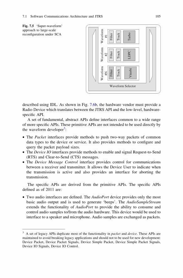
described using IDL. As shown in Fig. 7.6b, the hardware vendor must provide aRadio Device which translates between the JTRS API and the low-level, hardware-specific API.
A set of fundamental, abstract APIs define interfaces common to a wide rangeof more specific APIs. These primitive APIs are not intended to be used directly bythe waveform developer3:
• The Packet interfaces provide methods to push two-way packets of commondata types to the device or service. It also provides methods to configure andquery the packet payload sizes.
• The Device IO interfaces provide methods to enable and signal Request-to-Send(RTS) and Clear-to-Send (CTS) messages.
• The Device Message Control interface provides control for communicationsbetween a receiver and transmitter. It allows the Device User to indicate whenthe transmission is active and also provides an interface for aborting thetransmission.
The specific APIs are derived from the primitive APIs. The specific APIsdefined as of 2011 are:
• Two audio interfaces are defined. The AudioPort device provides only the mostbasic audio output and is used to generate ‘beeps’. The AudioSampleStreamextends the functionality of AudioPort to provide the ability to consume andcontrol audio samples to/from the audio hardware. This device would be used tointerface to a speaker and microphone. Audio samples are exchanged as packets.
Filte
r
Tra
ck
Tur
bo
Wav
efor
m
#1
Filte
r
Tra
ck
LD
PC
Filte
r
Tra
ck
Waveform Selector
Wav
efor
m
#2W
avef
orm
#N
Vite
rbi
Fig. 7.5 ‘Super-waveform’approach to large-scalereconfiguration under SCA
3 A set of legacy APIs duplicate most of the functionality in packet and device. These APIs aremaintained to avoid breaking legacy applications and should not to be used for new development:Device Packet, Device Packet Signals, Device Simple Packet, Device Simple Packet Signals,Device IO Signals, Device IO Control.
7.1 Software Communications Architecture and JTRS 105

• Since many JTRS radios are meant for voice communications, a vocoderinterface is one of the basic APIs. Vocoder Service API encapsulates vocodingcapabilities that are common across all waveforms and applications. TheVocoder Service API supports loopback operations, provides for the transfer ofencoded/decoded bit streams to and from the service user, and defines opera-tions to select algorithms supplied by the vocoder. It should be noted that the useof the base Vocoder Service API and codec extensions require an implicit orexplicit connection with the Audio Port device API. Implicit connections aredefined by the platform implementation. Explicit connections are defined usingthe Vocoder Audio Stream API Extension. The vocoder service is one of themore complex APIs.
• The Serial Port device provides the ability to send flow-controlled byte packetsto/from the device or service user and supports RTS/CTS handshaking. TheSerial Port device API also provides a base configuration interface. A specifictype of serial port is selected by using one of the extensions:
– Asynchronous extension defines a UART interface– Synchronous extension defines a synchronous serial interface– Synchronous High-Level Data Link Control (HDLC) extension extends the
functionality of the Serial Port to include synchronous serial capabilities usingHDLC [101].
• The Ethernet device abstracts the interface to an Ethernet network. It closelymirrors the low-level packet interface4 but adds Ethernet-specific addressingbased on unique MACs.
• The GPS device provides an interface to get the user’s position and/or time. Theformat of position and time information is set by deriving one of the twoextensions:
Waveform Application
Standardized APIs
OperatorInterfaces
ModemHardware
AudioHardware
NetworkInterfaces
Radio Hardware
JTRS API
Native API
(a)
RadioDevice
WaveformApplication
(b)
Fig. 7.6 Use of APIs in JTRS a conceptual view, b UML view
4 The Ethernet device is derived from the legacy Device Packet and DeviceIO rather than thenew Packet API (see footnote 3).
106 7 SDR Standardization
– Latitude/Longitude (LatLong) extension for radian latitude and longitudecoordinates.
– Military Grid Reference System (MGRS) extension for MGRS coordinates[102].
• Timing service maintains, manages, and distributes time within the JTR set. Thisincludes Terminal Time and System Time management and distribution. TheTiming service provides an interface for retrieving System Time and the qualityindicator, i.e., Time Figure of Merit (TFOM), for Terminal and System Time.Terminal Time is the time returned from the OS and is monotonicallyincreasing. Terminal Time is used for communicating time among the differentterminal components (including distributed processor software and hardwarecomponents). The Timing Service synchronizes the Terminal Time betweendistributed components within the terminal. The Timing Service controls thelocal processor’s POSIX clock. System Time is the terminal’s estimate ofCoordinated Universal Time (UTC) time. UTC time can be derived fromvarious combinations of inputs (e.g., the GPS device, the chronometer device,or operator input) while utilizing the local timing pulse. Note that the timingservice should be used in preference to getting the time from the GPS devicesince it is more general (e.g., timing may be available when GPS is not).
• Frequency Reference device provides the ability to read frequency referencedata and to set the GPS Time Figure of Merit (TFOM) value.
• Modem hardware abstraction layer (MHAL) modem hardware abstraction layerabstracts the modem interfaces from the application software. The MHAL APIsupports communications between application components hosted on GPPs,DSPs, and/or FPGAs. This API is described in more detail in Sect. 7.1.1.2.
7.2 STRS
SDR is very attractive for use in satellites and deep space missions. The radios onspace platforms have very long life cycles. As discussed in Sect. 3.6, changing thecommunications waveform can extend the life of a mission, increase the amount ofreturned data, or even save the mission from failure. NASA has been studyingSDR for the past 10 years and has also realized the need for a standard. Hardwaresuitable for use in space lags behind commercial hardware by at least 10 years.Thus, flight radios are significantly more constrained in terms of computationalresources than terrestrial equivalents. The SCA standard described in the previoussection is too heavy for implementation on most NASA missions (especially deepspace ones). NASA decided to develop a lightweight standard modeled loosely onthe JTRS standard, and called it ‘Space Telecommunications Radio System’ orSTRS [103].
7.1 Software Communications Architecture and JTRS 107

STRS has been in development since 2007 [92] and at least two flight exper-iments have been flown by 2011 with STRS-compliant radios. A conceptualhierarchical view of STRS components is shown in Fig. 7.7. Comparing this figurewith Fig. 7.1 clearly demonstrates that STRS is significantly simpler than SCA.Perhaps the largest difference is that no middleware layer (i.e., CORBA) is usedfor STRS.5 The bulk of the STRS standard deals with APIs. Unlike SCA, theSTRS standard also deals with hardware implementation of the radio. JTRSdevelopers were mostly concerned with application and waveform portability.STRS developers also want to be able to swap hardware boards between radios oradd new ones.
STRS developers learned from the problems encountered by SCA developerswhen integrating non-GPP components into the radio. STRS explicitly addressesthe ‘signal processing module (SPM)’ made up of ASICs, FPGAs, and DSPs thatdo not execute software. In fact, the GPP is meant for control only and is notexpected to do any signal processing at all.
The set of APIs defined by STRS is much smaller than for JTRS. Most of therequired APIs deal with the infrastructure and would be considered a part of theApplication Factory in JTRS. The API classes are:
• [Application Control] includes commands to interact with the waveform.Configure, start, stop, test, etc. This API is defined twice—one for the waveformlevel and one for the infrastructure level. The user only interacts with theinfrastructure, which in turn calls the waveform-level commands.
• [Application Setup] includes commands to prepare the application for execu-tion. Instantiate, remove, upload, etc.
• [Device Control] includes commands to interact with the hardware abstractionlayer. The HAL is not yet defined by STRS. Open, close, start, stop, etc.
• [Memory API] includes commands for generic memory allocation. Memory isoften a very scarce resource on flight radios and must be managed carefully.Further, NASA guidelines discourage dynamic memory allocation using the
Waveform Applications and High Level Services
POSIX API (subset) STRS API
STRS Infrastructure
Network Stack
Hardware Abstraction API
DriversBoard Support Package
GPP Module Specialized Hardware
OperatingSystem
Fig. 7.7 Conceptualhierarchy of STRScomponents
5 STRS does not require a POSIX-compliant operating system or CORBA, allowingimplementation of small- and low-power STRS radios.
108 7 SDR Standardization

standard ‘malloc’ function. Only three functions are defined in this API: copy,reserve, and release.
• [Messaging API] includes commands for a simple message passing architecture.Queues are used to send messages between threads in an application or betweenapplications. Both basic and subscriber-based message passing is supported.
• [Time Control] includes commands to get and set time.
The STRS standard is still a work in progress. STRS-compliant radios are likelyto facilitate easier waveform and application portability, but definitely do notguarantee it.
7.3 Physical Layer Description
The SCA and STRS standards deal primarily with waveform portability andprovide a waveform development environment. The actual waveform (physicallayer) is considered a black box6 that provides a means for sending or receivingbits. No open standard that addresses the physical layer is currently available.Consider the simple task of specifying the signal carrier frequency—some refer tothis parameter as fc, others as carrier, and others as freq. Multiple researchers haveidentified the need for such a standard [104,105,106], but their proposals did notcome to fruition and have not been accepted by the community. Another standard,SDR PHYsical layer description (SDRPHY), was proposed by the author of [107]to fill the gap by providing a lightweight description language that covers thesamples-to-bits part of the SDR. A crude analogy is: ‘‘SCA and STRS provide thebuilding codes and some of the materials. SDRPHY aims to provide the blueprints.Both are required to build a house’’. As of 2011, SDRPHY has not been acceptedby the SDR community or used beyond a few experimental demonstrations. Awebsite, http://sdrphy.org, has been established to allow open access to and col-laborative development of the standard.
A common language for describing waveforms for wireless communicationcan:
• Facilitate reuse of software developed for different hardware platforms.• Reduce the cost and time to move between different vendors’ solutions.• Stimulate research in software-defined and cognitive radios by simplifying
collaboration between different teams.• Reduce procurement costs by encouraging competition between vendors• Help students and researchers see the commonalities between different wave-
forms rather than focusing on the unique details.
6 The Application Factory in SCA does not know or care about the intent of the componentconnections defined in the SAD file.
7.2 STRS 109

Many of these goals are similar to the goals of SCA. However, SDRPHY is notan alternative to SCA, but is in fact complementary.
A software program, called an interpreter, provides an interface betweenSDRPHY and a specific SDR implementation. The interpreter converts thedescription into a set of configuration commands, or creates a flowgraph (e.g., anSCA SAD file), or even generates code to implement a radio satisfying thedescription. The interpreter may reside within the SDR hardware, or operateentirely offline. The interpreter should be able to:
• Report hardware capabilities.• Report current configuration.• Configure or reconfigure a set of options within the hardware capabilities.• Report current operating environment.• Provide a hardware-agnostic method to transmit and receive data.
The configuration, capabilities, and status are described using XML. A con-ceptual block diagram showing four different radios is given in Fig. 7.8. The mainconcept illustrated in the figure is a hardware-agnostic layer that allows multipleapplications to work with different SDR hardware. An application, which could beanything from a graphical user interface to a cognitive engine, generates XMLconfiguration files that are then passed to a hardware-specific interpreter.
These concepts are easily extensible to support cognitive radio, which is asuperset of SDR. The primary use of the standard is to exchange configurationinformation between the application and the radio. The two are assumed to beco-located or have some pre-established reliable means of communication.However, the standard can also be applied (with minor changes) to allow over-the-air exchange of capability information for cognitive radio negotiation. The standarddoes not address how an initial link between two cognitive radios is established.
Applications
XML Interpreter
XML parser
XML Interpreter
XML parser
SDR FPGAGNU Radio
Ethernet digitizer
XML Interpreter
XML parser
COTSModem
PCI bus Compile C++
Reportcapabilities
Setwaveform
Ethernet
XML Interpreter
XML parser
SCA::OSSIE
USB digitizer
Create SAD.xml
SDRPHYFiles (XML)
Fig. 7.8 Conceptual use of the XML standard
110 7 SDR Standardization
z

The XML format used to configure an SDR can also be used to describe users ina radio channel. For example, a cognitive radio detects RF emitters in the area andreports them as a set of SDR configurations.
7.3.1 Use Cases
Consider a ground station responsible for control and monitoring of multiplesatellites. Each satellite may use a different waveform. Currently a set of config-uration files in a proprietary format is used to setup the ground transceivers foreach satellite. A new satellite transponder is supported by developing a new set ofconfiguration files. Since the format is proprietary, it falls on the ground stationoperators to develop and test the configuration files. The satellite developer, who ismost familiar with the transponder, is unable to help. An agreed-upon standard forwaveform description would facilitate communication between them.
Consider a cognitive radio engine that can optimally select a waveform andcarrier frequency under different channel conditions. Developing such an engine isa major undertaking. However, if the software is designed for a particular SDRhardware platform, another major effort is required to port it to other platforms.A waveform description standard allows application portability. Further,two radios may exchange their ‘waveform capability’ descriptions and use anautomated method to determine the best mutually supported waveform. Currently,there is no standard way to exchange this information.
Consider a monitoring receiver that processes many different waveforms.Adding a new waveform currently requires knowledge of the receiver userinterface. Again, a standardized waveform description language is needed.
7.3.2 Development Approach
The goal of this standard is to provide a lightweight description language thatcovers the samples-to-bits part of the SDR. It is not meant to replace JTRS/SCA orSTRS but to augment them. In fact, configuration of an SCA-based SDR usingSDRPHY is described later in this chapter. The transmitter functionality starts withdata bits and ends at the antenna, while the receiver starts at the antenna and endswith data bits. In other words, only the physical layer is considered.
The standard should ideally satisfy the following goals
• Completeness Most practical waveforms should be describable using the stan-dard. The goal is for 99 % of all waveforms of interest to the user community tobe supported. The remaining 1 % of exotic waveforms may be overlookedbecause it would make the standard too complex.
7.3 Physical Layer Description 111

• Lightweight The interpreters for the standard are meant to be implemented in awide range of devices—from satellites to handheld units. Therefore, low pro-cessing and memory requirements are desirable.
• Consistency The standard should be self-consistent. Similar functionality shouldnot require different descriptions. A high-level, abstract view of the waveform isadapted whenever possible. Conceptual commonalities should be exploited.
• Compactness The same keywords should be used for describing the configu-ration and capabilities, whenever possible. In particular, no new keywordsshould be created if existing ones can be repurposed.
• Accessibility There should be no barriers to entry for users wishing to participatein the creation or utilization of this standard.
The consistency and compactness goals are currently being debated. There is atradeoff between using the most abstract view of a parameter and ease of imple-mentation and specification. Consider a Reed-Solomon (RS) error correctioncode—it can be shown that RS is a special case of a BCH code [108]. Therefore, itis sufficient to define a tag for BCH. On the other hand, many users of the standardmay not be aware of the equivalency between RS and BCH, placing an undueburden on them. One approach is to provide Reed-Solomon as a library entity,based on BCH. Similar tradeoffs come up in many other cases.
The goal of this standard is to enable application developers to work with awide range of practical flexible radios. The idea of a practical radio limits thescope of the standard: it does not attempt to describe an arbitrary radio. Somecombinations of features may be physically possible, but are either impractical orhighly unusual. For example:
A waveform may use either convolutional (Viterbi) or LDPC forward errorcorrection. It is possible to concatenate Viterbi and LDPC, but such a combinationmakes little sense from the communications architecture perspective. Likewise, itis possible to apply forward error correction to the chips in a spread-spectrumsystem instead of applying forward error correction (FEC) to the symbols. How-ever, no practical radio uses this technique.
The standard can therefore rely on a large set of implied constraints, based on acanonical communications system. These constraints are explicitly stated when-ever multiple interpretations of the XML are possible.
The implied constraints and the concept of a canonical system are an integralpart of the interpreter. It shifts some of the complexity of specifying a waveformfrom the application designer to the interpreter. For example, the applicationdesigner should be able to construct XML code to configure a radio by reading apublished standard. The complexity of such an interpreter can be a majorimpediment to adoption of the standard. The author implemented three such(admittedly limited) interpreters to demonstrate feasibility, as discussed in Sect.7.3.5. The same configuration file is passed to all radios and the radios canexchange data with each other.
There are at least two approaches to describe a waveform, but neither is fullysatisfactory:
112 7 SDR Standardization

1. Define constituent blocks and interconnections between them (apparentlyadapted by [105] and the SAD files for SCA). This approach comes close tospecifying the implementation rather than the intent. Once the block-basedparadigm is allowed, there is no logical reason why it cannot be extended tospecify every adder and multiplier in the system.
2. Specify values for all relevant system parameters (this is the approach used bymost published waveform standards). This approach is problematic due topossible ambiguities. For example if an FEC encoder and an interleaver areboth described, it is not clear in which order the operations should be applied tothe data.
The SDRPHY standard is mostly based on the second approach. Wheneverpossible, the goal is to describe the intent rather than the implementation. Most ofthe interconnect is implied by the canonical communications system. However,connectivity can be specified when absolutely necessary. Any constituent blockdescribed in XML can be uniquely identified with an ID attribute. Connectivity isspecified by adding a \input ID=‘‘unique_id’’[ node to the block fol-lowing the uniquely identified block.
Unique aspects of some systems cannot be adequately described using the XMLtags defined in this standard. For example, a spreading sequence for a DSSSsystem can be based on a proprietary cryptographic generator (e.g., GPS militarycodes). Describing such a generator is well beyond the scope of this standard. Aforeign attribute is therefore defined to allow the user to supply a non-standardcomponent. The foreign attribute is very problematic since it must be supportedacross different platforms—from software to hardware. The component interfacemust therefore be very well-defined and should be based on existing industrystandards (e.g., CORBA for software and Open Core Protocol (OCP) forhardware).
7.3.3 A Configuration Fragment
A comprehensive review of SDRPHY is beyond the scope of this book. Instead,one example is provided below and the reader is encouraged to explore the rest ofthe standard at http://sdrphy.org.
Most practical communications systems impose a packet and/or frame structureon the transmitted symbols. Let us consider an appropriate XML description forthe physical layer framing. The framing may be taken care of at the bit level (e.g.,older SATCOM signals), or may have to be managed at the symbol level (e.g.,DVB-S2). Some standards use different modulation and/or coding for differentparts of the frame.7 The frame structure for these standards must be described
7 This is also the case for OFDM waveforms, where the frame synchronization sequence is notnecessarily an OFDM symbol.
7.3 Physical Layer Description 113

before a transmitter or a receiver can be created. A frame structure that can behandled in the receiver at the data bit level (after hard decisions) need not bedescribed in SDRPHY.
A frame can be described as a sequence of fixed-duration segments (a segmentis the largest set of samples that can be processed at once). Each segment may bedescribed by a different waveform (e.g., a preamble may use a robust modulationsuch as BPSK, while the bulk data uses an advanced modulation). Most framesconsist of just two segments—preamble and bulk data. The preamble is typically(but not always) a combination of a fixed pattern and a short user-definedsequence. In particular, an FEC block must be contained within a single segment.(Fig. 7.9)
A frame is defined in XML as a sequence of segments. As with any XML forthis standard, the waveforms may be defined inside the segment definition, orreference previously defined waveforms. Three variables must be defined for eachsegment (see Sect. 7.3.7 for an example of their use):
• \duration[. Set the duration of the frame segment (in symbols) to betransmitted using the selected waveform.
• \data_source[. The data source selects one of: a named data source, a file,or a fixed data sequence.
– A named data source provides a standard way for the application to supplydata to the hardware.
• \waveform[. Define all the parameters of the waveform to be used for thesegment, such as: data rate, modulation, coding, etc.
Many waveforms insert known (pilot) symbols throughout the frame to helpwith acquisition and tracking. The pilots are inserted after FEC and can be thoughtto exist at the ‘frame’ rather than at the ‘segment’ level. The pilots are describedby their position in the frame and the symbol values at each position. SDRPHYreuses the concept of a segment to describe each block of pilots (frequently justone symbol). The\positions[ tag defines offsets for each set of pilot symbolsrelative to the first symbol in the first segment. If all the pilots are the same, onlyone \segment[ tag is used. However, if the pilots at different positions are notall the same, a separate\segment[ tag is required for each position. The framehierarchy is conceptually shown in Fig. 7.10.
Segment #1 Segment #2 Segment #N
One frame
e.g., preamble using BPSK fixed sequence
e.g., user data using 16-QAM turbo coded
Pilotsymbol(s)
Fig. 7.9 Canonical wireless data frame structure
114 7 SDR Standardization

7.3.4 Configuration and Reporting XML
XML has a number of advantages, the main ones being widespread acceptance andhuman readability. XML does come at a price since it is rather verbose,8 andtherefore requires more resources to generate, store, and parse than a custombinary format. However, this overhead is negligible, given the complexity oftoday’s SDRs.
An XML description consists of a hierarchical tree of nodes. Each node rep-resents a conceptual part of a waveform. The hierarchy is not always obvious. Ingeneral, node B is a child of node A if it satisfies the following question: Is B aproperty of A? For example: Does a radio consist of multiple transmitters andreceivers, or does each transmitter consist of multiple channels?
The top-level node is \radio[. The XML standard defines a companionconstraint language—an XML Schema Definition (XSD). The SDRPHY standardis itself an instance of an XSD file. Leveraging XML and XSD allows thedesigners to take advantage of a rich set of development tools. In fact, an XSD filecan be used to automatically generate a user interface suitable for definingwaveforms. SDR capabilities can also be reported as an XSD file by providing aset of constraints on top of the SDRPHY standard. For example, the standardspecifies that \modulation[ can be either \linear[ or \OFDM[. A capa-bilities report may restrict \modulation[ to be only \linear[. ExistingXML parsers can be used to verify that a given configuration file is valid for agiven capabilities file.
A set of standard libraries (e.g., defining ‘BPSK’, ‘rate 1/2 convolutionalencoder with K = 7’) are provided. These libraries can be used to create compactXML descriptions for common waveforms. A radio may be queried to list all thelibraries that it has already stored. Some radios may be able to save the uploadedlibraries so that they do not need to be resent with every XML file.
frame
duration
segment
data source
waveform
pilotpositions
segmentsegment
Fig. 7.10 SDRPHYhierarchy to describe a typicalwaveform frame
8 XML files can be compressed using the Fast Infoset (FI) binary encoding standard [255]. TheFI files may be further compressed using zlib. See [256] for a comparison of different XMLcompression strategies.
7.3 Physical Layer Description 115

7.3.5 Interpreters for Hardware-Centric Radios
Two proof-of-concept interpreters were developed to demonstrate the feasibility ofusing SDRPHY to configure a radio. The Comtech [109] modem uses SNMP toconfigure the hardware. The interpreter is a stand-alone program developed in C++that takes in an XML configuration file and outputs a stream of SNMP commandsto the modem. The capabilities file for the modem is created manually since thenumber of supported features is not very large.
The FPGA-based SDR is configured through a set of proprietary API calls. Alarge library of functions is used to configure everything from data rate to forwarderror correction to the frame structure. The number of options is larger than for themodem, but still quite manageable. The capabilities file is once again createdmanually.
For both the FPGA and the COTS modem, the interpreter follows a hard-codedflowchart to determine the appropriate SNMP commands or API calls. Very littleerror checking has to be done by the interpreter since an XML validator verifiesthat the configuration is within the radio capabilities. A fragment of a flowchart isshown in Fig. 7.11. At every node in the XML tree, the interpreter checks if it hasto issue an API call, or delve deeper before a call can be made.
7.3.6 Interpreters for Software-Centric Radios
An interpreter for an all-software radio is significantly more complex than for aCOTS modem. For example, GNURadio framework (see Sect. 8.1) allows creationof an essentially infinite number of different radio architectures. An advancedinterpreter may even create new functional blocks in C++ to satisfy the
<frame>
#(<segment>)=1
DisableHeader()
Y
SetHeader(<segment>[1].<data>)
N
<coding>
#(children)=0
end
Y
ProcessFEC(child[i])
N
Fig. 7.11 Sample flowchartto configure a modem
116 7 SDR Standardization

configuration file. However, the only requirement placed on any interpreter is thatit be able to configure a radio given an XML configuration file that satisfies thecapabilities report. The capabilities report is generated by the interpreter itself.9
Interpreters for two popular SDR frameworks, GNURadio and OSSIE, were cre-ated to demonstrate feasibility.
In GNURadio, each signal processing block (e.g., equalizer, phase locked loop)is defined as a C++ class. The connect method of each class is called to create afull receiver flowgraph. An SDR was designed using GNURadio framework bydefining several configurable blocks and a flexible connection between blocks. Inorder to be SDRPHY compliant, an interpreter was written in C++ to parse anXML file and then directly set the configuration variables for the SDR. Theinterpreter generates a unique build script that selects the subset of features set inthe configuration XML by defining preprocessor constants. For example, it sets themodulation and selects one of two FEC codecs. The front-end digitizer is con-figured based on the \carrier_frequency[ and the \symbol_rate[tags.
OSSIE is an SDR framework for implementing key elements of the SCAspecification (see Sects. 7.1 and 8.2). OSSIE is used to create waveforms con-sisting of multiple components that complete the radio. A component is a pro-cessing block that performs a specific function with the provided input. Acomponent can have properties set by the user. For instance an amplifier block hasa property specifying the amount of amplification. SCA defines two XML files(.sad, .prt) to determine how the components are connected and the property valuesfor each component.
An SDRPHY interpreter was developed in Python to generate these two XMLfiles. The interpreter begins by parsing the XML configuration file and keepingtrack of the tags it parses. Once it recognizes a tag that requires a component thatcomponent is added to the .sad file. It continues to interpret the children andattributes of that tag to set the appropriate properties for that component. Theprocess will continue until all tags have been parsed. At this point no connectionsbetween the components have been made yet. Connectivity between the compo-nents is implied by the canonical radio flow graph. If a component was notinstantiated during the parsing of the configuration file, it will be left out of thechain and no connections will be made to it.
The functionality of these interpreters was demonstrated by having each radiorelay a stream of packets over an RF connection to the other radios. The sameSDRPHY configuration files were used to configure the radios for differentmodulations, data rates, and FEC.
9 Incidentally, this approach limits the ‘vaporware’ claims of some SDR vendors that overstatethe capabilities of the radio. While it is true that firmware can be written to implement morewaveforms, the SDR as-sold only supports a finite set.
7.3 Physical Layer Description 117

7.3.7 Example
This section provides a relatively complete example demonstrating an SDRHYdescription of a DVB-S2 transmitter. Comments in the table apply to the XMLcode above them. (Table 7.1)
7.4 Data Formats
As long as the SDR is implemented by a single developer and is integrated on asingle board or chip, the format of the data exchanged between blocks is notimportant. In a hardware-centric architecture, digital samples can be exchanged onparallel buses. In a software-centric architecture, digital samples can be stored asarrays of appropriate data types. Data format becomes important when the pro-cessing is distributed between different entities and the entities are not co-located.Many radios implement mixed-signal processing and DSP on different chips.Consider a system shown in Fig. 7.12, where the analog signal is digitized in blockA and then processed in block B. At a minimum a standard is desirable for transferof data between these subsystems.
What if the data has some metadata attached to it? A typical example is atimestamp associated with a sample of data. Enforcing the data type between thesender and the receiver is not sufficient if data types are not uniform (e.g., samplesare floating point and timestamps are integers). Of course, ad hoc solutions can bedeveloped, where a separate connection is used to send metadata.
At least five standards to describe data exchange between SDR blocks arecurrently available (Table 7.2). Most of the time the data contains samples digi-tized at an intermediate frequency (IF, see Sect. 9.1.3). This proliferation isaddressed and justified in [110]. Each standard targets a narrow segment of themarket and implements only the minimal feature set required for that segment.High volume products such as RF front ends for handheld devices are extremelyprice sensitive and any extraneous features would make a product less competitive.However, as transistors keep getting cheaper, the incremental cost of imple-menting a full-featured standard decreases. Multiple standards will most likelyconsolidate or converge to just one or two.
7.4.1 VITA Radio Transport (VITA 49, VRT)
Modern military distributed systems rely on standard network infrastructure for allcommunication. Transfer of digital samples over a network can be standardized byrequiring a middleware layer such as CORBA (see Sect. 7.1.1.1). A middlewarelayer can be responsible for ensuring that the data type sent by the source is the
118 7 SDR Standardization

Sample configuration file
7.4 Data Formats 119

120 7 SDR Standardization

same as that expected by the sink (i.e., a floating-point value is not sent to a blockexpecting an integer). However, middleware is often not desirable (because ofsoftware complexity or overhead) or even feasible.
A platform- and middleware-independent standard for packetizing digitalsamples and attaching metadata to these samples is desirable. The VITA RadioTransport (VRT or VITA-49.0) protocol is an emerging standard for SDR appli-cations targeted at military users [111, 112, 113]. It was developed to provideinteroperability between a diversity of SDR components by defining a transportprotocol to convey digitized signal data and receiver settings. Unlike the SCAstandard, the VITA 49 is not particularly complicated or overarching. It onlydefines how data is to be packed into packets and states nothing about how it is tobe processed. It is not the only standard that addresses this issue, but is apparentlywinning the battle of the standards, as evidenced by the availability of hardware[114].
The VRT specification was developed for receivers only, and does notexplicitly support transmitters. This may appear as a major shortcoming but inpractice is not. Parameters required to describe a receiver are usually a superset ofthose required for a transmitter (e.g., power level applies to both received powerlevel and the transmit power).
VRT is meant to replace a set of analog IF cables and complicated analogswitch matrices with a standard and low-cost digital network running IP. Thevision [111] is encompassed in Fig. 6.34.
A
A/D
B
FPGA
X1 X2 XNtime X1 X2 XNtime
(a)
(b)
Standardize data exchange here
Fig. 7.12 Transmitting digitized data over a network a distributed computing demonstrates theneed for standard data format, b representative standard with timestamped data
Table 7.2 A summary of digital IF standards
Markets Supported standards PHY Cost
VITA 49 Military/space Agnostic N $100digRF High-volume chips Agnostic Y $8000SDDS Military/intelligence Agnostic N ?OBSAI Cellular basestations GSM/EDGE, WCDMA, LTE, WiMAX Y FreeCPRI Cellular basestations WCDMA, WiMAX, LTE Y Free
7.4 Data Formats 121

Two types of packets are defined (Table 7.3):
1. Data packets carry digitized samples and timestamps associated with thesamples. These packets are sent as data becomes available.
2. Context packets carry control and monitoring information. These packets aresent when the information changes (e.g., request to tune to a different fre-quency) or at a specified rate. Context packets are sent less frequently than datapackets and require little network bandwidth. The context information istimestamped so that changes can be precisely related to the associated data.
VRT also supports the transfer of other signal data in a customizable transportformat. This VRT protocol ‘extension’ capability supports any type of data thatneeds to be conveyed to handle a wide range of applications. For example, a VRTdata packet can be used to send soft decisions from a demodulator to an FECdecoder. VRT defines the term ‘information stream’ as a set of related packetstreams, typically at least one data stream and one context stream.
In order to associate the emitted VRT packets with VRT packet streams, eachemitted packet contains a stream identifier. The stream identifier is a uniquenumber assigned to a packet stream. The number is identical in all the packets of agiven packet stream. Stream identifiers are also used to associate together all of thepacket streams relating to an information stream. The context packets can beassociated with data packets in five different ways (data/context, source/context,vector/context, asynchronous-channel/context, system/context), but only the data/context association will be discussed in this section.
7.4.1.1 Data Packet Format
The VRT packet format is extremely flexible. In fact, only a 32-bit header isrequired. The header specifies any additional header fields. In particular, theheader specifies packet type (data, context, etc.), whether a stream identifier is
Table 7.3 VRT packet types
Contents Standard formats Custom formats
Data IF Data PacketConveys a digitized IF signal• Real/complex data• Fixed/floating-point formats• Flexible packing schemes
Extension Data PacketConveys any signal or data• Any type of data• Custom packet format
Context IF Context PacketConveys context for IF Data• Frequency• Power• Timing• Geolocation• etc.
Extension Context PacketConveys additional context• Any kind of Context• Custom packet format
122 7 SDR Standardization

available, and what type of timestamp is available. The packet length can be up to256 kB in 4-byte increments. A typical VRT data packet format is shownFig. 7.13.
Samples can be packed into 32-bit words either contiguously (with samplespotentially split across two words), or using padding to ensure an integer numberof samples per word. Each sample consists of the actual digital sample and twooptional qualifiers that describe an event10,11 that occurred at that sample.
The digitized samples can be either real valued or complex. Complex-valuedsamples can be expressed as either aþ ib or reih: Each component can beexpressed as either fixed- or floating-point number and either signed or unsignedwith 1—64-bit precision. Note that none of this formatting is explicitly describedin the packet header. Two mechanisms are provided to specify the sampleformatting:
1. An optional field called a class identifier selects a format from externallyprovided documentation (i.e., a vendor has to tell the user that packet class Xmeans samples are 8-bit signed complex values).
2. A context packet (see next section) may contain a data packet payload formatfield ([111], 7.1.5.18) that describes the formatting.
It is interesting to compare the almost arbitrary format of a VRT packet tothe strictly specified packets in the next subsections. The (overly) flexible nature ofthe VRT packets is a major impediment to the adoption of this standard outsidethe ‘cost is no object’ world of military users. Indeed, two systems that are both
Packet type
Time stamp in picoseconds is 4 ps after the GPS time in the previous field
First sample = 1 Second sample = 2 Third sample = 3 Fourth sample = 4
Time stamp in GPS format = 0x55555555 seconds
Packet length = 6 wordsPacket #1TSFTSI
Stream ID = 0x55
31 30 29 28 27 26 25 24 23 22 21 20 19 18 17 16 15 14 13 12 11 10 9 8 7 6 5 4 3 2 1 00 0 0 1 0 0 X X 1 0 0 1 0 0 0 1 0 0 0 0 0 0 0 0 0 0 0 0 0 1 1 0
0 0 0 0 0 0 0 0 0 0 0 0 0 0 0 0 0 0 0 0 0 0 0 0 0 1 0 1 0 1 0 1
1 0 1 0 1 0 1 1 0 1 0 1 0 1 1 0 1 0 1 0 1 1 0 1 0 1 0 1 1 0 1 0
0 0 0 0 0 0 0 0 0 0 0 0 0 0 0 0 0 0 0 0 0 0 0 0 0 0 0 0 0 0 0 00 0 0 0 0 0 0 0 0 0 0 0 0 0 0 0 0 0 0 0 0 0 0 0 0 0 0 0 0 1 0 0
0 0 0 0 0 0 0 1 0 0 0 0 0 0 1 0 0 0 0 0 0 0 1 1 0 0 0 0 0 1 0 0
Fig. 7.13 Typical VRT data packet (TSI—integer timestamp, TSF—fractional timestamp)
10 Events can also be indicated in an optional trailing word ([111], 6.1.7) or in a context packet.11 Sample format can have a significant effect on the performance of the GPP-based SDR. GPPsare designed to work with a few standard data types (e.g., 8-bit chars, 16-bit shorts, 32-bitintegers, 32-bit floats, and 64-bit doubles). Further, high performance is achieved only whenworking on blocks of data rather than single samples. Interleaving flags and data samples requirethe GPP to ‘unpack’ the data before it can be operated on.
7.4 Data Formats 123

VITA 49 compliant may be unable to exchange data if they do not support everypossible variation of the packet format.
7.4.1.2 Context Packet Format
Context packets are used to convey metadata that describes samples in the datapackets. Context packets are not needed in the simplest systems. When contextpackets are used, the stream identifier is used to link data packets to the corre-sponding context packets. VRT defines 24 types of metadata (e.g., signal band-width and carrier frequency) that can be sent in a standard context packet.
One of these 24 types describes the data packet payload format and is criticalfor interpreting the associated data packets. This field describes formatting (e.g.,unsigned 8-bit fixed point) and packing (e.g. continuous) of the sample data. Ifclass identifier is not used to interpret the data format, at least one context packetmust be received before any data packets can be processed.
Context packets can be transmitted without any associated data packets. Forexample, an RF downconverter can send out a context packet indicating its carrierfrequency. The output of the downconverter is analog. A digitizer (ADC) thenconverts the analog signal to digital samples and generates VRT data packets. TheADC may also generate its own context packets, indicating the sample rate. Theuser can form a complete picture of the system by considering context packetsfrom both the downconverter and the digitizer. As discussed previously, thecombination of the two context packet streams and the data packet stream is calledan information stream.
7.4.1.3 Packet Loss Mitigation
VITA 49 does not specify the physical or MAC layers. Standard Ethernet networkinfrastructure is envisioned for most implementations. The packets may be lostwhile traversing multiple switches and routers. The effect of a lost packet on theoverall system performance depends on the details of the system. Infrequentpacket loss may be booked against the target end-to-end BER and ignored, or itcan be catastrophic if an entire user transmission is lost. MAC layer retransmissioncan be employed if the additional latency is tolerable (e.g., using TCP/IP) and thehardware is fast enough to support TCP/IP at the packet rate. To the best of theauthor’s knowledge, all VITA 49 systems use the unreliable UDP protocol ratherthan TCP. Packet-level forward error correction can be used to compensate for lostpackets at the cost of slightly higher throughput requirements [115]. Timestampsembedded in the packets can be used to detect dropped and out-of-order packets.
124 7 SDR Standardization

7.4.2 Digital RF (digRF)
The digRF standard is developed by MIPI alliance [116] to address the require-ments of high-volume commercial products for the broadband wireless market.This specification defines the interface between one or more DSPs and RF frontends in a single terminal. The interface is intended to be efficient, flexible, andextensible, accommodating many variations in the overlying system design, whileproviding interoperability at the interface level between compliant ICs. digRFspecifies everything from the names given to IO pins on the chips to the voltagelevels used to the packet formats. This level of detail is needed to ensure com-patibility between different vendors. The VITA49 standard described in the pre-vious section addresses only the packet format, and is agnostic to the physicallayer. Standard specification is made available only to MIPI members at a cost ofabout $10 k. Therefore, it is not appropriate for R&D institutions. The limitedinformation available in the public domain and not under NDA comes from [117].Six IO pins are defined for bidirectional data transfer between the chips, as shownin Fig. 7.14. Tx and Rx data are transferred serially using high-speed (up to1.5 Gbps) differential signaling. The high line rate is derived from a lower fre-quency reference clock (typically 26 MHz), using a PLL inside both RF and DSPchips. The maximum line rate supports signal bandwidth up to about 75 MHz.12
Data are transferred in packets of up to 64 kB in size. Each packet can carryeither I/Q samples or control information. This approach is similar to that used byVITA49.
7.4.3 SDDS
SDDS is an old format for the exchange of digitized sampled signals used widelyin the military community. It is now being replaced by VITA 49 and is onlydescribed here for completeness.
SDDS packets are always encapsulated inside standard UDP packets and sentover the Ethernet networks [118]. The packet format is shown in Fig. 7.15. SDDSoffers a few unique features:
DigRFCore
Clockmultiplier
DigRFCore
Clockmultiplier
Clk_En
RxData
SysClk
TxDataRFIC
A/D
D/A
Clock reference
RFF
E
BasebandIC
Fig. 7.14 digRF physicallayer
12 (1.5 9 109 bps)/(8 b/sample)/(2 samples/Hz) * packet overhead *75 MHz.
7.4 Data Formats 125

• Accurate specification of the digitizer sampling clock. Not only is the nominalfrequency specified in every packet, but the rate of change of that frequency isspecified as well. These two pieces of information can be used to very accuratelyrecreate the digitizer clock.
• Two timestamps are generated
1. Specify the UTC time for the first sample in the packet2. Specify the sample within this packet that occurred on a 1 ms boundary. The
1 ms time tag is used to create time tags for even older standards (Datoliteand SDN)
• Two low-rate data streams are interleaved with the primary sampled data.
1. A synchronous serial data stream (SSC) consists of one data bit that transi-tions infrequently (no more than once per packet) to mark a specific sample.The sample number at the transition is sent with every packet. The signifi-cance of the marks is not specified (e.g., could indicate that the antenna wasmoved).
2. A 19.2 kbps asynchronous data stream (AAD) is used to provide ‘side’information about the main data stream (compare to the context packetsdescribed in Sect. 7.4.1). The meaning of the data stream is not specified.
Simple packet-level error correction is explicitly supported. Every 32nd packetcan contain parity data over the preceding 32 packets. This allows the system tocorrect any single packet that is in error out of the 32 packets.
PreambleEthernetHeader
IP PacketEthernet
FCS
IP HeaderUDP
HeaderData & Signal Information
FormatIdentifier
FrameSeq. #
DataTime Tag
Info.SSC Info. SSD Info. AAD Info.
2 Bytes2 Bytes 16 Bytes 1024 Bytes
8 Bytes 1108Bytes 4 Bytes
1080 Bytes20 Bytes
IP PacketLevel
Payload
1134 Bytes
EthernetLevel
14 Bytes
12 Bytes 4 Bytes 20 Bytes
8 Bytes
Fig. 7.15 SDDS packet format
126 7 SDR Standardization

7.4.4 Open Base Station Architecture Initiative
The OBSAI family of standards was developed to address interoperability betweensubsystems in a wireless base station. A modular base station architecture assumedby OBSAI is shown in Fig. 7.16. The interfaces between subsystems are known asreference points (RPs). Digital IF interface between the DSP and mixed-signal/RFis described in RP3 and RP3-01 [119]. RP3-01 extends RP3 by adding a way tosend control messages from the control block (RP1) to the remote RF block.Unlike digRF, which defines yet another standard for the physical layer, OBSAIleverages existing standards.13 At the highest line rate, the link can support onesignal with bandwidth up to 100 MHz or multiple narrower band signals [120].
Since OBSAI was developed to support commercial base stations, the standardhas explicit support for popular wireless standards: GSM/EDGE, WCDMA, LTE,WiMAX. Packet formats are described to transport digital IF samples for eachstandard. Every packet contains the type field and a timestamp. Timestamps arerequired to make packet-based digital IF transfer work. For OBSAI, the timestampis interpreted differently for uplink (base station receiver) and downlink (basestation transmitter):
• In the uplink direction, a timestamp identifies the time instant when the lastsample of the message was available at the output of the channelizer block(down-converter, FIR filter).
• In the downlink direction, a timestamp defines the time instant when the firstsample of the payload must be inserted into the modulator (up-converter, FIRfilter) (see also discussion in Sect. 6.1 and Fig. 6.3).
Interpretation of the timestamp also depends on the packet type (i.e. wirelessstandard). For example, a WCDMA timestamp refers to the index of the chip in atimeslot. For WiMAX, timestamp refers to the sample number in a frame.
The packet payload also depends on the packet type. For example, downlinkWCDMA samples use 16 bits to encode I and Q components of each chip, sampledonce per chip, while the uplink uses 8-bit values sampled twice per chip. The
TransportBlock
BasebandBlock
RFBlock
LocalConverter
Remote RF Block
RP3
RP3-01
Fig. 7.16 Base station architecture for OBSAI
13 OBSAI goes one step further than digRF and specifies even the mechanical connectors, butthat part of the standard is not relevant to this section.
7.4 Data Formats 127

dozen or so different formats are clearly not sufficient for a general SDR. It isinteresting to note that all formats specify baseband sampled data (I/Q) rather thanIF sampled. Thus, technically, OBSAI cannot be considered a digital IF standard—only a digital baseband standard.
A large part of the standard is devoted to specifying frequency stability, fre-quency accuracy, and all the delays in the system (including delays through RFcables). Very tight tolerances are required to support multi-antenna techniques.This level of specification is not provided in VITA 49 standard, but is absolutelynecessary to support MIMO operation.
7.4.5 Common Public Radio Interface
The CPRI standard was developed by a consortium of competitors14 to the con-sortium that developed OBSAI. CPRI also addresses the cellular base stationmarket and supports most of the same wireless standards as OBSAI [121]. CPRIwas initially developed to support only the WCDMA wireless standard. Since thenit has been expanded to support WiMAX and LTE as well. True to its single-purpose roots, CPRI specifies not only the format of the data exchanged betweenDSP (known as REC in CPRI documentation) and RF (known as RE) blocks, buteven the exact partitioning of the radio. As shown in Table 7.4, the RF block startswith pulse shaping. This level of specificity makes CPRI unsuitable for a genericSDR.
Similar to OBSAI, all of the data formats assume baseband (IQ) sampling.However, different sample precision is supported (4–20 bits for uplink, 8–20 fordownlink) and the oversampling ratio can be either 1 or 2. The additional sample-level flexibility requires more complicated packet formats than OBSAI. The data issent over a high-speed serial link with line rates up to 10 Gbps in multiples of
Table 7.4 Partitioning ofDSP and RF subsystems inthe CPRI documentation
Downlink Uplink
Pulse shaping Matched filteringD/A conversion A/D conversionUpconversion DownconversionOn/Off control of each carrier Automatic gain controlCarrier multiplexing Carrier de-multiplexingPower amplification Low-noise amplificationAntenna supervisionRF filtering RF filteringMeasurements
14 Ericsson, Huawei, NEC, Nokia Siemens Networks and Alcatel-Lucent.
128 7 SDR Standardization

614.4 Mbps. The fundamental line rate was chosen to work well with WCDMAstandard, but requires stuffing of dummy bits to support WiMAX.
Control and management (C&M) data is time interleaved between the IQ datapackets. Two different layer 2 protocols for C&M data—a subset of High-levelData Link Control (HDLC) and Ethernet—are supported by CPRI. These addi-tional control and management data are time multiplexed with the IQ data. Finally,additional time slots are available for the transfer of any type of vendor-specificinformation.
7.4 Data Formats 129

Chapter 8Software-Centric SDR Platforms
GPPs have become fast enough to implement all of the DSP for practical radios.As discussed in Sect. 5.1, an all-software radio is considered the holy grail of SDRdevelopment [122]. Presently, the two most popular open-source SDR platformsare GNURadio and OSSIE. In this section, we will explore these platforms in somedetail.
8.1 GNURadio
GNU Radio (GR) is an open-source framework for designing SDRs. The majorcomponents of GR are:
1. A framework for an arbitrary signal processing block that can be connected toone or more other blocks.
2. A scheduler responsible for activating each processing block and managingdata transfer between blocks.
3. C++ and Python infrastructures to build up a flowgraph from multiple blocksand attach the flowgraph to the scheduler.
4. A relatively rich set of frequently used DSP blocks such as filters, trackingloops, etc.
5. A graphical user interface (GUI) that allows the user to create GR designs bydrag-and-dropping blocks and drawing connections between them (see Fig. 8.1).
6. An interface to a commercial hardware front end. The front end hardwareprovides the interface between the GPP and the physical world. It containsmixed-signal (ADC, DAC) and radio frequency (up/downconverter) compo-nents (see Sect. 8.4.2).
GR waveforms are designed using datapath architecture (see Sect. 6.4.2), whichis ideally suited for processing streaming data because data is transferred betweenblocks via streams. A packet-based interface using message queues is available,but is not intended for transferring real-time data samples.
E. Grayver, Implementing Software Defined Radio,DOI: 10.1007/978-1-4419-9332-8_8, � Springer Science+Business Media New York 2013
131

Most of the signal processing blocks are developed in C++. The blocks can beinterconnected, and complete GR applications can be created using either C++ orPython. Python is an interpreted1 (rather than a compiled) language, and is gen-erally considered to be easier for development and debugging. All the visualizationblocks (e.g., scope, spectrum) provided with GR rely on the Python developmentflow. True to its open-source roots, GR is best supported on Linux (and MacOS),with less support for Windows.
8.1.1 Signal Processing Blocks
A block is the fundamental unit of a waveform developed using GR. A block maybe as simple as a multiplier (a.k.a. gain), or as complex as an FEC decoder. Ablock is characterized by its inputs, outputs, and the ratio (r) of the input rate to theoutput rate.
A block can have an arbitrary number of input and output ports, with the actualnumber determined once the flowgraph is built.2 Input and output ports can eachbe of a different data type (e.g., floating point, complex value, etc.) with differentsample rates. Three special types of blocks are identified:
Fig. 8.1 GNURadio Companion graphical user interface (GRC)
1 An open-source software tool called SWIG is makes blocks developed in C++ available inPython.2 For example, an ‘adder’ block can be declared with an arbitrary number of inputs and oneoutput. The block can then be used to sum up multiple data streams, with the number of streamsdetermined at runtime.
132 8 Software-Centric SDR Platforms

1. Source blocks have no inputs and one or more outputs2. Sink blocks have no outputs and one or more inputs3. Hierarchical blocks contain one or more basic blocks.
All GR blocks must be derived from one of these fundamental types:
1. gr_block allows arbitrary r, and r can change over time2. gr_sync_block requires r=1 on all ports3. gr_sync_decimator requires r=N on all ports, where N is an integer4. gr_sync_interpolator requires r=1/N on all ports
The block name should end in a suffix that indicates the data types it consumesand generates.3 The suffix consists of one, two, or three characters. The firstcharacter denotes the input data type, the second character denotes the output datatype, and the third character denotes the coefficient data type for filters. Charactersfor standard data types are listed in Table 8.1. A few examples are given inTable 8.2.
The structure of a gr_block is shown in Figure 8.2. The key componentsupplied by GR is the output buffer. The output buffer is a thread-safe single-writer, multiple-reader circular buffer. The user-defined work(…) function pro-cesses data from the input ports and puts the output into the buffer(s). Data arepassed to the work function as an array of abstract items. Note that before the inputdata can be processed, it must be cast into the appropriate data type (e.g., integer).
Each item can be annotated with an unlimited number of metadata ‘tags.’4 Atag is defined by a tuple {name, value, origin}, where the name is a stringdescribing the tag, and value can be of any data type.5 The origin field isoptional and is meant to convey which block generated the tag. For example, theseventh item on input N in Figure 8.2 is annotated with the time (0.0123) that itemwas captured. Three tag propagation options are available:
Table 8.1 Characters that describe data types for GR blocks
Character Type
b Bytes Short (2 bytes)i Integerf Single precision floating pointc Complex floating pointv Modifies the subsequent character to indicate a vector of that type
3 The naming convention is not enforced and some blocks do not follow it.4 Only a few items are expected to be tagged since tags are processed much slower than the itemsthemselves.5 GR defines an abstract polymorphic type, pmt_t. This type acts as a container for arbitrary datatypes (e.g. doubles, floats, structs, arrays, etc.).
8.1 GNURadio 133

1. Copy tags from ith input to ith output. This is the default option and is onlyapplicable if the number of inputs is equal to the number of outputs.
2. Copy tags from all inputs to all outputs.3. Do not copy any tags automatically. The user can then write code to selectively
propagate and optionally modify tags.
Automatic tag propagation correctly handles the input/output ratio. For examplea 1:10 interpolator propagates an input tag for item n to output item n 9 10.
Once all downstream blocks have completed processing a range of data, thewrite pointer in the circular buffer is advanced. This simple and elegant archi-tecture allows a programmer to concentrate on the signal processing and not worryabout transferring data between blocks.
In addition to items and tags, a block can send and receive messages. Messagesare similar to tags in which they can contain arbitrary data. Unlike tags, messages
Table 8.2 Samples of the GR block naming convention
Block name I/O description
gr_sig_source_s A signal source that outputs ‘shorts.’ Note that a source block has only onetype associated with it.
gr_vector_sink_b Converts input ‘byte’ stream to a vector of bytes. Note that a sink block hasonly one type associated with it.
gr_add_ff Adds two or more streams of floats to generate a float outputgr_add_const_vcc Adds a complex valued constant vector to an input vector of complex values.gr_fft_vfc Computes an FFT of an input vector of floats and output a vector of complex
values.gr_fir_filter_ccf A filter with floating point coefficients processes complex input and generates
a complex output.
bufferInput 1
buffer
block 1
work(…)function
block 2
block 3
scheduler
item
item
item
item
item
item
item
item
item
i tem
i tem
item
“time”
0.0123
tag
Input NOutput 1
Output M
Fig. 8.2 Anatomy of a gr_block
134 8 Software-Centric SDR Platforms

are asynchronous, i.e., messages are not tied to items. Messages are typically usedto exchange data between a top-level GUI or control application and the blocks.6
To create a new GR block, the user must be familiar with C++ and optionallywith Python. The block is developed in C++ and must define only one function,work(), that implements the actual signal processing.7
The work function consumes the bulk of computational resources and musttherefore be efficient to meet real-time processing throughput. Some frequently usedblocks (e.g. filters, FFT) provided with the GR framework are optimized to takeadvantage of special instructions available on modern processors (i.e., hand-codedin assembly to utilize SIMD instructions). However, most of the blocks are written instandard C++ and rely on the compiler for any optimization. In the author’sexperience, simply using a processor-specific optimizing compiler such as the onefrom Intel increased the throughput for a simple radio by a factor of two. Evengreater improvement can be achieved by using highly optimized libraries providedby the processor vendor (e.g., IPP and MKL from Intel [123], ACML from AMD,and others). Modifying the work function of most GR blocks to take advantage of theIPP library increased the throughput by a factor of four8 (see Sect. 8.1.4).
8.1.2 Scheduler
The current GR scheduler is multithreaded9—each block runs in a separate thread,with its own mini scheduler [124]. The overhead due to switching between manythreads and handling the semaphore locks on the data buffers is negligible as longas many samples are processed every time a block is activated.10 The schedulerkeeps track of how much space is available in the block’s output buffers and how
6 The top-level GUI or control application can also call member functions of the blocks directly.Messages provide a higher level interface that is guaranteed to be thread-safe. Messages alsomake it easy to control radios that execute on multiple computers.7 Many blocks also define functions to set parameters at runtime (e.g., set the gain on a‘multiply’ block).8 The performance improvement is strongly dependent on the coding style. GR developers areactively working on integrating processor-specific optimizations into the GR baseline. The latestversion of GR provides a library of hand-coded assembly functions called VOLK to takeadvantage of modern processors [287]. Users can expect baseline GR performance to improve,making it closer to what is achievable with an optimizing compiler and vendor libraries.9 Older versions of GR used a single threaded scheduler.10 This constraint is not always easy to achieve. Multiple blocks generating and consuming dataat different rates cause ‘fragmentation.’ Fragmentation means that the scheduler calls the workfunction with only a few samples. Larger sample sets can be enforced by setting a minimumnumber of samples a block can accept. The problem is exacerbated if feedback loops existbetween blocks. The author has observed scenarios where 90 % of the CPU time was spent in thescheduler itself rather than in the work functions. These anomalous conditions are difficult toidentify and debug.
8.1 GNURadio 135

much data are available from the upstream blocks. The scheduler then tries tomaximize the amount of data processed at once. The block activation schedule is afunction of space in the buffers and the sample rate change introduced by eachblock. This form of flow control is known as event-driven, where an event from anupstream block initiates processing in downstream block(s). For example:
• Block 1 has 1,000 samples in its output buffer• Block 2 has 500 free samples in its output buffer• Block 2 is an interpolator with r = 4.
Block 1’s scheduler wakes up block 2’s scheduler to tell that data are available.Block 2’s scheduler calls its work() to process min(1,000, 500/4)=125 samplesfrom block 1. The scheduler also takes care of passing messages between blocksusing message queues. The scheduler is automatically created when the userderives a top-level block from a gr_top_block class, as shown in Fig. 8.3.
8.1.3 Basic GR Development Flow
GR is installed from a binary package available for Linux or Windows, or builtfrom source code. Documentation is very sparse, even for an open-source project,and the developer has to be prepared to learn by example. A number of exampledesigns are provided in the source code to demonstrate many fundamental fea-tures, mostly for Python and a few for C++.11 One of three development flowsmust be selected: (1) Python, (2) C++, (3) Graphical (GRC). The GRC flow has thelowest learning curve and is recommended for relatively simple designs. Pythonflow is recommended if the developer is familiar with that language. C++ flow canbe used if the developers are not familiar with Python, or need a completely stand-alone application that does not rely on Python.
block 3
block 5(sink)
block 4block 1(source)
block 2
block 6(sink)
gr_top_block
data and tags
GUI or other control application
message queues
Fig. 8.3 GR top-level block and control application
11 More full-featured examples are available at the GR archive network (GRAN) at https://www.cgran.org.
136 8 Software-Centric SDR Platforms

Starting with a system block diagram of the desired radio, the developer mustidentify which blocks12 are already provided with baseline GR distribution.Documentation for each block is entirely in the C++ header file for that block andvaries from nonexistent to comprehensive. Blocks that are not provided in thedistribution have to be created by either writing C++ code or by combiningavailable blocks. While it is possible to build up blocks from many primitiveblocks (e.g. add, multiply, mux, etc.), the resulting design is very difficult to readand typically results in lower throughput. For any relatively complex radio, thedeveloper will have to write one or more blocks from scratch.
File source and sink blocks are used extensively during debugging. Theseblocks capture intermediate and final signals to disk for post processing. Forexample, a single block can be debugged by creating a flowgraph consisting of afile_source, block_under_test, and file_sink.13 Real-time debugging is supportedby a combination of graphical output blocks (scope, spectrum) and file sinks.
In general, it is difficult to estimate the maximum throughput based on theflowgraph. GR documentation does not provide any benchmark data. If theprocessor cannot keep up with real-time throughput, the hardware interface blockswill output under/overflow warnings. Classical software performance improve-ment techniques can be applied to increase throughput. A high-quality profiler(e.g. VTune or gprof) is invaluable in identifying the bottleneck blocks.14
8.1.4 Case Study: Low Cost Receiver for Weather Satellites
The Geostationary Operational Environmental Satellite R-series (GOES-R)satellite [125] is being developed by National Oceanic and Atmospheric Admin-istration (NOAA) to provide the next generation of weather data. One of themissions of GOES-R is to provide support for future versions of the EmergencyManagers Weather Information Network (EMWIN) and Low-Rate InformationTransmission (LRIT) signals [126, 127]. The current signal bit rates are below300 Kbps. GOES-R increases the rates to 1 Mbps. The cost of upgrading groundstations, especially for developing world countries, is a major concern for NOAA.NOAA developed an SDR to demonstrate the feasibility of a low-cost terminal thatcan be used to receive both GOES-R and legacy signals [64].
GNURadio was selected for this effort since it is open source and does notincrease the cost of the receiver. A number of new blocks were designed todemodulate and decode EMWIN and LRIT satellite signals. All the new blocks
12 A mostly complete list of fundamental blocks is available at http://gnuradio.org/doc/doxygen/modules.html.13 GR development guidelines suggest using automatic regression testing for every new block.14 Common sense is usually insufficient. The author came across a design where the noisegeneration block took significantly more computational resources than a Viterbi decoder. Alsosee footnote 10 in this chapter.
8.1 GNURadio 137

follow GR block architecture design and can be shared with other GR developers.Many blocks from baseline GR distribution were redesigned to use Intel IntegratedPerformance Primitives (Intel IPP) for improved performance [123].
The only incremental cost (versus an existing ground station) is a front endcapable of digitizing the new, wider band signals. A custom digitizer designed forthis effort, described in Sect. 8.4.2.1, can be built for \$100.
The next sections describe some of the signal processing required to demod-ulate three signals of interest: LRIT-BPSK, EMWIN-OQPSK, EMWIN-FSK.
8.1.4.1 Frequency Acquisition
The constituent blocks of the acquisition engine are shown in Fig. 8.4. Each blockin the figure corresponds to a GR block executing in a separate thread. All the blocksexcept for the gr_freq_acq are part of the standard GR distribution. Frequencyis acquired by finding a peak in the averaged fast Fourier transforms (FFTs) of thesignal. The search window (frequency uncertainty), resolution, and amount ofaveraging are all runtime programmable. An Nth-power detector is used to removemodulation from the subcarrier. Peak search is run once the desired number FFTshave been averaged. The acquisition engine returns locations and powers ofdetected peaks. Since the signal can fall between FFT bins, experiments show thatconsidering multiple adjacent bins improves acquisition accuracy. The acquisitionresult is used to adjust the frequency of the downconverter in the digitizer.
8.1.4.2 BPSK and OQPSK Demodulation
A conventional receiver with separate phase and timing tracking loops wasimplemented to demodulate BPSK and OQPSK signals (Fig. 8.5). A Costas phasetracking loop removes any frequency offset remaining after acquisition and alignsthe phase. A Mueller–Muller timing tracking loop [128] aligns the sampling time
From H/W
N
gr_fir_filter
( )2serial-to-
parallelFFT
Accumulate
subcarrier
gr_mixer
gr_multiply
gr_stream_to_vector gr_fft_vcc gr_freq_acq
NCO
Find peaks
Fig. 8.4 Block diagram of the frequency acquisition engine
138 8 Software-Centric SDR Platforms

to the peak of every symbol. The symbols are then processed by a Viterbi decoder.Designing a software Viterbi decoder to handle the data rate of 900 kbps waschallenging. The decoder supports any constraint length, rate, and polynomial.Since the specifications of the GOES-R broadcast signal are not completelydefined, the advantage of having a flexible decoder outweighs the potential forhigher throughput from a fixed decoder. The initial design was able to maintain athroughput of 300 kbps. The algorithm was vectorized to take advantage of theIPP functions and throughput increased to 1.9 Mbps.
8.1.4.3 FSK Demodulation
Some of the data from older weather satellites is transmitted with FSK modulation.FSK is very robust and may be available even when signals described in theprevious section cannot be received. The FSK signal encodes an asynchronouswaveform that closely mimics the serial interface used in dialup modems. A blockdiagram of the FSK demodulator is shown in Fig. 8.6. The symbol decisionmetrics are created by correlating the received signal with two locally generatedtones, corresponding to the two transmitted tones. The magnitude of the output ofthe correlator, implemented as an integrate-and-dump block, is sampled at symbolboundaries, and a hard decision is made. The FSK demodulator does not requireany frequency tracking since the front end is assumed to compensate for largefrequency offsets. Small frequency offsets have a negligible effect on the overallperformance of the system. The FSK symbol timing is acquired by looking for a‘01’ sequence transition, and then tracked using the same algorithm as for BPSK.
gr_costas_loopgr_agc
Matchedfilter
gr_clock_recovery
gr_binary_slicer
To bitsink
T/2
Freq.Acq
LPF
gr_fir_filter
Vite
rbi
deco
der
gr_viterbigr_diff_decoder
gr_deinterlave
FromHardware
M&MTED
DiffDec.
gr_fir_filter
gr_delay
gr_freq_acq
NCO
Dei
nter
leav
e r
Fig. 8.5 Block diagram of the BPSK/OQPSK demodulator (shaded blocks only for QPSK)
8.1 GNURadio 139

8.1.4.4 Results
The implementation of a complete receiver for three different live signals dem-onstrates that GR is suitable for deployment and is not just for experimentation.The lost cost, very flexible receiver demonstrates some of the advantages of SDR.The front end digitizer supports legacy signals as well as proposed signals, and hasenough bandwidth for future signals as well. The entire development effort tookless than 2 man-years, which is significantly faster than implementing the samereceiver(s) in an FPGA or ASIC.
8.2 Open-Source SCA Implementation: Embedded
Open-source SCA implementation—embedded (OSSIE) is an open-source plat-form for developing SCA-compliant (see Sect. 7.1.1) radios.15 At first glance it issomewhat similar to GNURadio in that it also allows a developer to create andinterconnect signal processing blocks. While GR was developed from the groundup by a team of dedicated amateurs for quick-and-dirty experimentation on abudget, OSSIE complies with a standard developed by the military at a cost ofbillions. GR assumes it is running on a Linux variant and has direct access to thefile system and hardware. SCA waveforms run in a well-specified operatingenvironment, with the file system and hardware abstracted by an API. Blocks inGR are interconnected using explicit Python or C++ commands and samples aretransferred using custom circular buffers. OSSIE uses XML files to define theconnectivity, and the actual connections are accomplished using CORBA services.More importantly, samples are transferred over the ORB, using TCP/IP. In par-ticular, the ORB allows different blocks to execute on different machines, while
DDS
gr_mixer
N
Fromfront-end
gr_fir_filter
DDS
gr_mixer
I&D
Tone #1
Tone #2
Timing Tracking
Diff.dec
Acquisition
gr_binary_slicer
gr_clock_recovery_mm
Fig. 8.6 Block diagram of the FSK demodulator
15 In this section, SCA and OSSIE will be used interchangeably.
140 8 Software-Centric SDR Platforms

GR flowgraphs are meant to execute on a single machine.16 Since ORB is ageneral purpose software bus and is not specific to SDR, the concept of a‘scheduler’ does not really apply to an SCA waveform. Samples are transferredover the ORB and basic flow control is used to start/stop transfers.
The main goal of GR is providing the signal processing framework, while themain goal of OSSIE is providing an SCA operating environment.
These differences and similarities have led to significant confusion and somedevelopers still regard GR as a competitor to OSSIE [129]. In fact, the OSSIE teamhas recently demonstrated an SCA-compliant waveform that relies on GR for signalprocessing. A GR flowgraph is encapsulated inside an SCA component [130].
It is quite feasible to develop a complete radio in OSSIE, although the set ofsignal processing blocks provided with the baseline distribution is significantlysmaller than for GR.
The OSSIE distribution includes:
• A GUI (based on the popular Eclipse platform) to select and interconnect blocks(see Fig. 8.7). Note that the connections between blocks are indicated by iconsinstead of lines (TxDemo_1 is connected to RxDemo_1).
• A GUI to define new blocks. This GUI creates the skeleton C++ files that mustthen be modified by the developer to add the desired signal processing code.17
Fig. 8.7 OSSIE GUI for defining waveforms
16 It is relatively easy to build an application in GR that runs on multiple computers. Forexample, the UDP source/sink blocks can be used to transfer samples between machines.However, this approach is ad hoc, versus the well-defined ORB architecture.17 Only the: ProcessData() function is modified to implement the desired signal processing. Thisis very similar to modifying the: work() function in a GR block.
8.2 Open-Source SCA Implementation: Embedded 141

For example, a component shown in Fig. 8.8 has an output (uses) port named a,an input (provides) port named y, and a configurable parameter called p.
• A GUI to examine and debug waveforms (applications). This GUI allows thedeveloper to monitor (scope, spectrum) interblock signals. Monitors can beadded at runtime (unlike GR, which requires all the monitors to be definedbefore the flowgraph is started). The debug view of the application defined inFig. 8.7 is shown in Fig. 8.9.
Fig. 8.8 OSSIE GUI for creating new components
Fig. 8.9 OSSIE GUI for viewing and debugging application
142 8 Software-Centric SDR Platforms

• A fully SCA-compliant CORBA based on the open-source omniORB.• A set of tutorials and laboratory exercises. OSSIE is distributed as a ready-to-
run virtual machine. A Windows user can download the distribution and executeit without having to install Linux. Simple installation and tutorials make itsomewhat easier to get started with than GNURadio.
8.3 Other All-Software Radio Frameworks
GNURadio and OSSIE are by far the most popular open-source SDR developmentplatforms.
There are a few commercial products that compete with OSSIE. The popularSpectra system from Prismtech [131] provides a complete environment fordeveloping SCA-compliant waveforms. It comes with a high-performance COR-BA implementation and is geared toward military-grade waveform development.Prismtech offers a complete solution, including a hardware front end tightlyintegrated with the software. One of the unique features of the Spectra frameworkis support for native FPGA implementation of a subset of CORBA features (seeSect. 7.1.1.2). This FPGA-based CORBA allows components to be deployed onFPGAs without the use of proxies or other hardware abstraction layers (HALs) thatimpose additional memory and processing overhead. Other SCA frameworkvendors include L3 Communications, BAE Systems, Harris, and CRC [132]. CRCprovides both a commercial and open-source SCA framework.
There is no direct commercial equivalent to GNURadio.18 Simulink fromMathworks can be used to create flowgraphs that implement SDR. In fact, Simulinksupports the same hardware front end as GR. However, Simulink is a more generalpurpose environment and is much slower than GR for implementing even moder-ately sophisticated waveforms. The Microsoft Sora framework is a quasi-commercial competitor to GNURadio and will be discussed in the next section.
8.3.1 Microsoft Research Software Radio (Sora)
Many corporations have robust in-house SDR research efforts. Some have decidedto leverage GNURadio, while others are building frameworks from scratch.
18 The venerable X-Midas (multiuser interactive digital analysis system for X-windows)framework is a quasi-open-source alternative to GNURadio. X-Midas has been in developmentsince the 1970s and is used exclusively by the intelligence community. It is only available toqualified users from the government. X-Midas provides most of the functionality available in GR,and a simple wrapper can be created to make GR blocks execute ‘as-is’ in X-Midas. A paralleldevelopment from the X-Midas community is available to the general public [288].
8.2 Open-Source SCA Implementation: Embedded 143
Microsoft has released some information about their in-house SDR frameworkcalled Sora [133]. Unlike GNURadio, Sora is only available to academic institu-tions, is not licensed for commercial use, and is not open source. Similar toGNURadio, Sora consists of a library of prebuilt signal processing modules and ananalog front end. Unlike GR, which focuses on standard and portable code, Soraaims to achieve the highest possible throughput by taking advantage of everyavailable optimization. The key optimization technique used by Sora is mappingcomplex mathematical operations into precomputed lookup tables. Once the tablesare initialized, each operation is very fast as long as the tables fit within theprocessor cache. One example is a soft demapper (also known as a slicer), whichconverts the received complex symbols into soft decisions suitable for FECdecoding. Performance-critical signal processing code is optimized to use pro-cessor-specific single instruction multiple data (SIMD) instructions. Since theSIMD registers on Intel processors are 128-bit wide while most PHY algorithmsrequire only 8 or 16-bit fixed-point operations, one SIMD instruction can perform8 or 16 simultaneous calculations!
Just like GR, Sora uses a scheduler to activate each signal processing block andpasses data between blocks. However, unlike GR, the Sora scheduler uses a staticschedule optimized for the particular flowgraph. The number of circular buffersbetween the blocks and the number of threads is therefore much smaller than foran equivalent GR flowgraph.19 For optimal processor utilization, the number ofthreads should be the same as the number of cores, as long as each thread can beguaranteed to use all of the core’s resources. Threads are mapped to dedicatedcores to minimize cache thrashing. The Sora architecture reduces performancepenalty when processing small blocks of data. GR performance plummets whenthe block size falls below 512 bytes.
The results presented in [133] show that Sora can achieve about 109 higherthroughput than a similar GR implementation. However, FEC decoding is still amajor bottleneck—even the relatively simple Viterbi decoder requires a dedicatedcore. Today’s GPP is still not fast enough to decode powerful modern codes [134].
8.4 Front End for Software Radio
The SDR frameworks described in this chapter all require an interface to the ‘realworld.’20 As discussed in Chaps. 2 and 9, all practical radios today require an RFand mixed-signal front end. Custom hardware is usually developed for radiosintended for commercial or high volume. A front end is usually integrated with aGPP on a single circuit board to meet the mechanical requirements of the radio.
19 A static scheduler also avoids data the fragmentation problem discussed in footnote 10 in thischapter.20 Unless the SDR is used for simulation rather than for actual communication.
144 8 Software-Centric SDR Platforms

Radios intended for research and development typically leverage COTS solutions.Describing commercially available products in a book is a losing proposition sincethey are invariably obsolete by the time the book is published. The hardwaredescribed in this section is meant to represent different classes of front endsavailable to SDR developers rather than endorse any particular solution. Somesolutions provide only the mixed-signal front end and require additional hardwarefor the RF front end. Separating mixed-signal from the RF allows the user to mix-and-match products and select the best combination for each radio. However,recent availability of inexpensive wideband RF hardware has made integratedsolutions possible.
8.4.1 Sound-Card Front Ends
The simplest and lowest cost mixed-signal solution is already available in all PC inthe form of the sound card. A high-end sound card has A/D and D/A converterscapable of digitizing *40 kHz of bandwidth and can therefore support somenarrowband waveforms (e.g. AM or FM radio, some amateur radio signals). Soundcard-based SDRs are used primarily as educational tools [135, 136], but have alsofound practical application [137]. An RF front end is not required for basicexperimentation, and two sound cards can be connected directly to each other.21
The amateur radio community offers a few RF front ends designed to interfacedirectly to a sound card [138] for under $200.
8.4.2 Universal Software Radio Peripheral
Introduction of the Universal Software Radio Peripheral (USRP) brought down thecost of SDR experimentation from tens of thousands to hundreds. The USRP is acommercial product initially developed by a one-man shop that was then acquiredby National Instruments. USRP was released at about the same time as GNURadioand has been well integrated into that framework. In an unusual developmentmodel, the source code for USRP drivers and the mixed-signal circuit board are inthe public domain, while RF circuit boards are proprietary. USRP is now alsosupported in Simulink [139] and LabView [140]. The first generation of USRPsrelies on the USB2 interface and provides up to &30 MHz of instantaneousbandwidth for about $1000 (Fig. 8.10b). The second generation moved to gigabitEthernet and provides up to 50 MHz of bandwidth for about $2000 (Fig. 8.10c).
21 The signal could even be sent over the air, but an enormous antenna is required to efficientlytransmit a 15 kHz carrier (wavelength = c/15e3=20 km). Practically, a smaller antenna wouldwork at the cost of reduced SNR.
8.4 Front End for Software Radio 145

Different daughter boards are used to support a wide range of RF frequencies, withalmost continuous coverage from DC to 6 GHz. Each USRP supports two receiveand two transmit channels,22 and multiple USRPs can be synchronized to providemore coherent channels. The USRP consists of an FPGA, 100 MHz-class A/D andD/As, RF daughter board(s), and an interface to the host computer (Fig. 8.10a). TheFPGA is used to channelize the data and interface to the host port. The Ethernetinterface on the USRP2 supports the VITA-49 standard discussed in Sect. 7.4.1.
The FPGA implements digital frequency shifting and rate change. The FPGAsource code can be modified to implement more sophisticated processing. Forexample, multiple channels can be digitized in parallel and sent to differentcomputers on the network. Some or even all23 of the DSP for the SDR can beimplemented on the FPGA to achieve higher throughput than is possible with a PC[141]. One version of the USRP2 integrates a GPP and DSP into the chassis andcan be used to implement a completely stand-alone SDR.
8.4.2.1 Low-Cost USRP Clone
A clone of the USRP1 was developed to address the need for a low-cost receiver.The receiver was developed by The Aerospace Corporation as a proof of conceptfor the next-generation satellite weather station (see Sect. 8.1.4). A stripped-downUSRP1 includes a single receive-only channel and an integrated RF front end. Thisdevice, shown in Fig. 8.11, has a bill of materials under $100.
USB2 or GbE
A/DA/D
A/DD/A co
nnec
tor
RF daughterboardRF daughter
board
(a)
(b) (c)
DDSK
M
FPGA
Fig. 8.10 Universal software-defined radio peripheral (USRP). a Block diagram. b First-generation (USRP1). c Second-generation (USRP2)
22 First-generation USRP provides four A/D and D/A channels, but RF daughter boards supportonly two.23 The FPGA is relatively small and is not suitable for complex DSP such as FEC decoding.
146 8 Software-Centric SDR Platforms

Two front end interfaces were designed:
1. An IF interface for 140 MHz carrier frequency. This interface can be connectedto an existing downconverter. The downconverters are available at all currentground stations to support legacy receivers.
2. An RF interface for 1.688 GHz carrier frequency. This interface is intended fornew ground stations.
The input to the digitizer is assumed to have been received by a satellite dishand downconverted from radio frequency (RF) to an IF in the range of140 ± 6 MHz. Figure 8.11 shows the overall composition of the receiver. Since140 MHz is a popular commercial IF frequency, this allows us to use a low-powerand inexpensive A/D and also provides for noise filtering using an inexpensivesurface acoustic wave (SAW) input filter. To suppress out-of-band thermal noise, a12 MHz wide SAW filter was used as a first element in the receiver chain.Insertion loss of the filter has negligible effect on the SNR since the signal hasalready been boosted by the LNA. Out-of-band noise is also greatly suppressedand will not be folded into the signal in the sampling process. The bandwidth ofthe filter was chosen to be larger than the bandwidth of the signal to accommodatethe gamut of different weather satellite signals that may be of interest to the user.The SAW filter is followed by an automatic gain control (AGC) block whichrestores and keeps the signal level at an appropriate 2 Vpp differential level for theADC. The AGC provides gain from -2.5 to +45 dB. The ADC used in the designhas 12-bit resolution and a sampling rate of 48 MHz. The 140 MHz input signal issubsampled at 48 MHz. This technique allows us to relax the front end require-ments for the digitizer since high frequency clocks and filters would increase the
AGC
DDS
M
IF137.5 MHz
SMA
12 MHz @140 MHz
FPGA
FIFO
USBController
A/D
48 MHz
USB
40 MHz @1688.42 MHz
PLL1.5NF, 12 dB LNA6.5 NF 13dB Mixer
Fig. 8.11 Block diagram of a low-cost, receive-only USRP clone
8.4 Front End for Software Radio 147

cost of the board. To minimize the overall cost of the digitizer, a single clocksource is used on the board. As described previously, the signal is downconvertedand decimated in the FPGA prior to transmission over the USB interface.
Components used in the USRP are too expensive to achieve NOAA’s goal tobuild a receiver that could be manufactured for around $100. In order to reducecosts, dual ADC/DAC was replaced with a single ADC. The clocking network wasoverhauled so that only a single crystal is used instead of two crystals and aphased-lock loop (PLL). This crystal provides a clock reference for everything onthe board while using the PLL inside the USB controller. A single receiver designfits on a smaller FPGA than the one on the USRP, reducing its cost by half. Thecomponents of the current board cost around $80, and even less if mass productioncost reduction is considered.
The complete design consumes about 1.5 Watts and is powered entirely overthe USB port. The board is enclosed in a metal box which reduces electromagneticinterference (EMI) emissions. The device also includes a set of LEDs to indicatethe power of the input signal. The user can use the LED measurement as afeedback system to measure the incoming signal amplitude while adjusting theposition of the satellite dish. This board features SPI and I2C interfaces for internalcontrol. All of these functions can be accessed through the general softwareinterface, and most of the internal devices can be controlled in the same way.
Fig. 8.12 Network-based RF front ends
148 8 Software-Centric SDR Platforms

8.4.3 SDR Front Ends for Navigation Applications
A few relatively low-cost RFFEs are available for developers working in thenavigation bands (L-band). The low-cost SiGe front end [142] was made popularby an excellent book on software-defined navigation receivers [143]. NSL Stereosupports both navigation and non-navigation bands [144]. These and similardevices are suitable for implementing SDR receivers, but do not provide transmitcapability.
8.4.4 Network-Based Front Ends
USRP is the most popular and by far the lowest cost general purpose SDR frontend. From its inception, the USRP has been targeted at R&D rather than fordeployment. Two representative front ends, shown in Fig. 8.12, are intended forfield use and are available from thinkRF [114] and Rincon [145]. The thinkRFdevice includes both RF and mixed-signal subsystems, while the Rincon devicerequires an additional RF downconverter. Both devices provide only receiverfunctionality. The thinkRF device uses VITA-49 output, while Rincon uses theless common SDDS. These and other solutions [146, 147] are targeted at militaryand law enforcement users, and are about 5 times more expensive than a similarlyconfigured USRP.
8.4 Front End for Software Radio 149

Chapter 9Radio Frequency Front End Architectures
A wideband flexible radio frequency front end (RFFE) is needed to implement anSDR. As discussed in Chap. 2, the RF front end is the most challenging problem ina truly universal radio. In this chapter we consider some high-level tradeoffs inexisting RF front end architectures and how they apply to SDR. The tradeoffs forreceivers and transmitters are quite different. The transmitter is typically simpler toimplement and will be considered first. As a point of reference, a modern cellulartelephone RFFE, shown in Fig. 9.1, has dedicated circuitry for each of thesupported bands.
9.1 Transmitter RF Architectures
A transmitter must generate an electromagnetic wave at sufficient power to ensuresufficient SNR at the receiver. The low-level signals generated inside the radio areamplified by a power amplifier (PA). The PA usually consumes more power thanany other block in the radio. A PA is often a discrete chip since it requires adifferent fabrication processes than low-power components. The input to the PAshould contain only the desired signal because it is wasteful to amplify signals andthen filter them out. PA efficiency is defined as the ratio of output power toconsumed power. Narrowband amplifiers are more efficient than wideband ones,but are not suitable for SDR since they restrict the range of supported carrierfrequencies. Advanced signal processing can be applied to improve efficiency byoperating the amplifier closer to its limit [149].
The next few subsections discuss a few techniques for converting digitalsamples to an RF waveform. These techniques are applicable to a wide range ofwaveforms and therefore suitable for SDR.1
1 Techniques applicable to only one class of waveforms (e.g., constant envelope) will not bediscussed. For a more detailed discussion see [222].
E. Grayver, Implementing Software Defined Radio,DOI: 10.1007/978-1-4419-9332-8_9, � Springer Science+Business Media New York 2013
151

9.1.1 Direct RF Synthesis
The basic purpose of the transmitter RFFE is to take the digital samples computedin the baseband subsystem and convert them to an RF waveform at the desiredcarrier frequency. The RF waveform is then converted to an electromagnetic waveat the antenna. The simplest transmitter RFFE is based on direct RF synthesis asshown in Fig. 9.2. The DSP subsection implements a digital frequency synthesizer(DDFS) with an effective2 clock rate at least twice the desired carrier frequency,Fc. The DAC sample rate, Fs, must be3 greater than 2 9 Fc. The spectrum of thegenerated signal is shown in Fig. 9.2. Aliases of the desired signal occur atmultiples of the sampling frequency, and must be filtered out before the poweramplifier (PA). Note that as Fc approaches Fs/2, the separation between the desiredsignal and the alias decreases, requiring a sharper filter. Practical constraints on the
Fig. 9.1 RFFE interface for a multi-mode cellular phone [148]
2 The actual clock rate can be much lower if multiple parallel paths are used.3 This is not strictly the case since aliases of the primary signal in the higher Nyquist regions canbe used [269]. However, practical concerns such as output power and passband flatness limit theuse of Nyquist regions higher than 3.
152 9 Radio Frequency Front End Architectures

filter sharpness limit the maximum supported Fc to well below Fs/2. The advan-tages of direct RF synthesis are:
• Reduced number of components, leading to a more compact implementation andpotentially lower cost.
• Fewer sources of noise and distortion.• Very agile frequency synthesis allows the radio to jump from one frequency to
another with almost no delay. This feature is especially important for cognitiveradios and some wideband frequency-hopped (see Sect. A.4.9) systems.
Direct RF synthesis is rarely used in today’s radios due to the followingdisadvantages:
• High sample rate is required for the DAC. For example, a 2.4 GHz carrierrequires at least 5 GHz sample rate. DACs at this sample rate do exist (see
D/A
DDS
BasebandDSP
Digital
0 Fs/2
Desiredsignal
Fc
PA
Undesiredalias
Fs-Fc
Fig. 9.2 Direct RF synthesis for the transmitter
Digital
BasebandDSP
D/A
D/A
PA
Mixed signal RF
0 Fs–Fs 0 Fs–Fs 0 Fc
Fig. 9.3 Zero-IF upconversion with an optional (dashed-line) output filter
9.1 Transmitter RF Architectures 153

Sect. 10.2.4), but are expensive and draw a lot of power. Higher carrier fre-quencies cannot be generated directly because no adequate DACs are available.
• High-speed DACs provide lower accuracy and dynamic range (fewer bits) thanlower speed versions. High dynamic range is required for modern waveformssuch as OFDM. Even more dynamic range is required if the transmitter supportsmultiple simultaneous users with very different power levels.
9.1.2 Zero-IF Upconversion
In a zero-IF architecture, an IQ mixer is used to translate the complex basebandanalog signal to a desired carrier frequency. The name zero-IF refers to the factthat the input signal is centered on DC (0 Hz). Two DACs are used to generate theIQ components of a complex baseband signal, as shown in Fig. 9.3.
The mixer is usually a passive device. It internally creates a 90� shifted replicaof the reference carrier (local oscillator, LO) and multiplies the I input by the LOand the Q input by the shifted replica. The sum of the products gives the basebandsignal translated to the carrier frequency (Fig. 9.4). The ideal version of thiscomponent, known as an image-reject or quadrature-IF mixer, does not generateany additional spectral images and does not require filtering. However, practicalbroadband mixers create spectral images at each multiple of Fc and may requireadditional filtering before the PA.
The advantages of this architecture are:
• Baseband and DACs operate at a rate proportional to the bandwidth of thesignal, not the carrier frequency. Lower sample rate results in reduced powerconsumption and possibly lower cost.
• Since two DACs are used to create the signal, each DAC must be sampled atonly 19 the signal bandwidth rather than 29. Zero-IF is the only way togenerate very wideband signals that exceed the bandwidth of a single DAC.
• Very high carrier frequencies can be supported with minimal increase in powerconsumption. IQ mixers are available for carrier frequencies from low MHz towell over 50 GHz, with a single device covering multiple octaves.
90° hybrid
sin
cos
I
Q
LO
IQ mixer
RF
Fig. 9.4 IQ mixer
154 9 Radio Frequency Front End Architectures

• Filtering can be very simple, with just two fixed-frequency lowpass filters at theoutputs of the DACs to remove images above the DAC sampling frequency.Assuming a high-quality IQ mixer, no RF filtering is required.
• IQ mixers can be implemented in standard semiconductor processes and can beintegrated with the DACs and even filters on a single chip.
The disadvantages are:
• The gain and phase for I and Q branches have to be matched very closely toachieve image rejection. A slight imbalance results in the appearance of aspectrally inverted image on top of the signal of interest.
• Any DC offset at the I or Q inputs results in LO leaking through to the RF port.• Semiconductors introduce a lot of noise around DC due to a process known as
‘flicker noise.’ For narrowband signals this noise can significantly degradeoverall SNR.
• A synthesizer is required to generate appropriate LO. The LO power level has tobe fairly high (e.g. +10 dBm) to drive a passive mixer. The synthesizer cantherefore burn a lot of power. An active mixer can be used, but also requires anontrivial amount of power
• Two DACs are required instead of just one. This is a minor concern since dual-channel DAC chips are widely available.
• More circuit board space may be required for the two filters, synthesizer, andmixer. However, highly integrated (single chip) solutions exist.
The first two problems can be corrected in the digital baseband. If a feedbackpath is available to detect the presence of I/Q imbalance or LO feedthrough, thedigital I and Q signals can be appropriately modified (e.g., by adding a smallnegative bias to the DAC input with a positive DC offset). The feedback may bealways present for contiguous compensation, or may only exist during post-fab-rication testing on the assembly line. In the latter case, RF output is measuredusing standard test equipment over the expected operating temperature range.Compensation coefficients are calculated and loaded into the DSP subsystem.
9.1.3 Direct-IF Upconversion
Direct-IF upconversion relies on the DAC to generate a signal at a low interme-diate frequency (IF) and a regular mixer to translate the IF frequency to the desiredcarrier (Fig. 9.5). This architecture is an obvious extension of the direct-RFsynthesis described above, but for higher carrier frequencies. The DAC is sampledat a rate proportional to the IF frequency rather than the carrier frequency.
The advantages are:
• Generating a signal at an IF frequency avoids ‘flicker noise’ that plagues zero-IFarchitectures.
9.1 Transmitter RF Architectures 155

• DC offset in the DAC can be filtered out by the second bandpass filter, reducingthe need for calibration.
• A simple mixer can be used4 instead of a more complicated IQ mixer, possiblysaving power.
The disadvantages are:
• An RF bandpass filter is required to remove the image at FLO–FIF.5 Dependingon the desired carrier frequency range, the filter may need to be tunable.
• All of the disadvantages of zero-IF upconversion.
D/A
DDS
Bas
eban
d
Digital
IF
PA
0 Fs/2FIF Fs 0 Fs/2FIF Fs
0 +FIFFLO–FIF 0Fc=FLO+FIF
A
A
B
B
C
C D
D
Fs-FIF
FLO=Fc-FIF
Fig. 9.5 Direct-IF upconversion
4 A version of the IQ mixer, known as the Hartley Mixer, can be used to avoid the secondbandpass filter. A Hartley mixer internally creates I and Q branches from the real-valued inputsignal, and then uses a standard IQ mixer.5 Alternatively, the image at FLO ? FIF can be removed. The remaining image is then spectrallyinverted. Using high-side vs. low-side image provides a degree of freedom in the frequency planof the radio. Interesting work reported in [292] proposes filter-less direct-IF upconversion basedon polyphase combining.
156 9 Radio Frequency Front End Architectures

9.1.4 Super Heterodyne Upconversion
Any of the previously described architectures can be extended by adding more RFmixers before the power amplifier (Fig. 9.6). The additional mixers are used totranslate the signal to successively higher carrier frequencies. This approach isused when no single-stage components are available for the desired carrier fre-quency, or when the RF filter design becomes impractical.6 For example, mixersfor 100 GHz band do not work with baseband or low-IF inputs, but require inputsabove one GHz. A 100 GHz transmitter would then use one of the architecturesdescribed above to upconvert a signal to, say, 2 GHz. The upconverted signal isthen mixed with a 98 GHz LO to arrive at the desired 100 GHz carrier.
9.2 Receiver RF Front End Architectures
Receiver RFFE architectures are very similar to transmitter architectures. How-ever, the tradeoffs are somewhat different. The main difficulty in designingwideband and flexible receiver front ends is the existence of adjacent channelinterferers. Most (but not all) transmitters are only concerned with generating asingle signal, usually of modest bandwidth. However, the receiver has to contendwith all signals received by the antenna. As discussed in Chap. 2, it is notunreasonable for the desired signal to be adjacent to an interferer that is a billiontimes stronger.
Low-RF (IF) modulator
PA
0F 1 0
A B
A
B
FLO2=F2-F1 C
FLO3=Fc-F21
F2
F1
F2 Fc
0
C
Fc
Fig. 9.6 Three-stage super hederodyne upconversion
6 The Q-factor of the RF filter is roughly proportional to Fc/FIF since the filter has to remove animage 2 9 FIF away from the signal of interest, centered at Fc.
9.1 Transmitter RF Architectures 157

A receiver must protect the signal of interest from interferers at every point inthe receive path. This can be achieved with a combination of filtering (whichreduces interference) and/or high dynamic range (which allows the DSP to removeinterference). The tradeoff between dynamic range (required to linearly process thesignal of interest and all interferers) and filtering (which removes the interferers) isfundamental to receiver RFFE design. High dynamic range requires all compo-nents in the receive chain to be very linear and the ADC to have high resolution(making them expensive and increasing power consumption). Filtering is prob-lematic because tunable filters are not yet widely available (see 10.4).
Receiver architectures closely mirror the transmitter architectures (direct RFsampling, zero-IF downconversion, IF downconversion, and super heterodynedownconversion) will not be discussed for conciseness.
9.2.1 Six-Port Microwave Networks
Six-port microwave network is a technology developed in 1970s that has beenrecently repurposed for wideband, high frequency SDR RFFE [150, 151]. The ideabehind six-port RFFE is to obtain multiple observations of the downconvertedsignal in the RF domain and then apply signal processing to extract the desiredsignal. It is somewhat similar to direct-IF conversion, but with more than twobaseband signals. As shown in Fig. 9.7, four ADCs are used to digitize themagnitude (not the amplitude) of four downconverted versions of the signal. Eachversion is downconverted with a different phase. The additional observation allowsDSP to compensate for mismatches in the RF components. The microwave net-work can be implemented in a compact and low-cost chip if the carrier frequencyis high ([10 GHz). For lower carrier frequencies, the size of the six-port networkis quite large. Obviously, the additional ADCs also contribute to the cost andpower consumption. To the best of the author’s knowledge, this technique has notbeen implemented in any commercial SDR RFFE.
RFSplitter
90°Coupler
90°Coupler
Hybrid
0°
90°
()2
()2
()2
()2
A/D
A/D
A/D
A/D
Dig
ital I
Q r
egen
erat
ion
I
Q
1 2
3
4
5
6
Fig. 9.7 Six-port RFFE receiver (ports are numbered)
158 9 Radio Frequency Front End Architectures

Chapter 10State-of-the-Art SDR Components
The state of the art in digital and RF components changes much faster than neweditions of this book can hope to track. This section aims to capture the com-mercially available technology at the end of 2010 and is likely to be woefully outof date by 2015. However, even if technology has advanced, many of the trendsand approaches described here will remain valid for a few more years.
The term ‘state-of-the-art’ must always be qualified by the specific market theart is addressing. Three broad market segments can be identified:
• Consumer-grade radios that are manufactured in high volumes and must berelatively low cost. For the purposes of this section, both cellular phones andmilitary handheld radios are included in this segment.
• Research and development test equipment represents the high end of what ispossible in the commercial marketplace. Cost is not entirely irrelevant, but issecondary to performance. These devices are hand built in low volume andextensively tuned and calibrated for optimal performance.
• Exotic, one-of-a-kind radios developed for the military represent the true state-of the art. Technology in these devices may never trickle down to consumers.
The cost of a single device increases exponentially in each market segment.A consumer-grade radio may cost of the order of $100; test equipment setup costs$100,000; and a radio on a military satellite can exceed $10,000,000.
10.1 SDR Using Test Equipment
The author has found that a good way to extrapolate what technology will beavailable for consumer-grade radios in 5–10 years is to look at the currentlyavailable test equipment. Test equipment includes instruments such as digitaloscilloscopes, spectrum analyzers, and signal generators. Development of test
E. Grayver, Implementing Software Defined Radio,DOI: 10.1007/978-1-4419-9332-8_10, � Springer Science+Business Media New York 2013
159

equipment is market-driven and is targeted at current and upcoming wirelessstandards. It is not driven by the desirements1 of SDR researchers.
10.1.1 Transmitter
A signal generator is essentially a very configurable transmitter, and is an excellentplatform for an SDR. Two aspects of a signal generator must be considered: signalbandwidth and range of carrier frequencies. Since most current wireless standardstarget signals with less than 100 MHz of bandwidth, most signal generators also donot support higher bandwidth. The most flexible transmitter requires two pieces oftest equipment: an RF signal generator to create the carrier tone, and an arbitrarywaveform generator to create the baseband signal (see Fig. 10.1). The two are thencombined using one of the upconversion architectures described in the previouschapter. The mixer can be internal to the RF signal generator or a simple externalcomponent. Two representative instruments are described in Table 10.1. Note thatthe very wide carrier frequency range is not covered instantaneously—switchingfrom one frequency to another takes a few milliseconds.
Arbitrary waveform generators (AWG) for bandwidth below 200 MHz areavailable from many vendors and can be built into the RF signal generator. Thisbandwidth is sufficient for the vast majority of SDR applications. Options for verywideband operation are more limited, and two examples are described inTable 10.2. Note that these wideband models are designed to play back a fixedlength sequence and do not provide a way to supply an external, contiguous datastream (low bandwidth models do have this capability). However, the existence ofthese AWGs means that an equivalent DAC can be integrated into an SDR.2 Thewideband AWG can be used to generate the signal directly at the carrier frequency(for Fc \ 10 GHz), without using an RF signal generator.
Fig. 10.1 Representative wideband SDR transmitter using Agilent test equipment [152]
1 Desirements are an apt term for parameters that are highly desirable, but not required.2 Theoretically, it is possible to take apart the AWG and interface directly to the high-speedDACs.
160 10 State-of-the-Art SDR Components

A power amplifier may be required to complete an SDR transmitter based onstandard test equipment. The RF signal generators typically output no more than+20 dBm. This output level is sufficient for emulating handheld devices, but isinadequate for long-distance communications. A very wideband power amplifierwould be required to cover the full range of carrier frequencies supported by thesignal generator. To the best of the author’s knowledge, no such power amplifier iscurrently available. A set of separate amplifiers can be used instead, with a switchto select the desired band.
10.1.2 Receiver
A very flexible receiver can be constructed using either an oscilloscope or aspectrum analyzer (see Fig. 10.2). The oscilloscope setup closely follows theRFFE receiver architectures described in the previous chapter. The oscilloscopecan be used to directly sample the RF signal if the sample rate and dynamic rangerequirements are met. Alternatively, a signal generator (see previous section) isused to generate the desired carrier frequency and downconvert the signal ofinterest before it is sampled with an oscilloscope.
Modern oscilloscopes offer very high sample rates, but relatively low dynamicrange. Two representative examples are described in Table 10.3. The first oscil-loscope belongs to the class of general purpose devices and offers relativelylimited bandwidth (well below half of the sample rate). The second belongs to theclass of high-speed serial link analyzers and offers a very wide bandwidth. At firstglance, it may appear that wide bandwidth oscilloscopes can be used to implementthe ideal SDR by sampling directly at RF. However, the limited dynamic rangemeans that adjacent channel interferers will drown out the signal of interest. Thesedevices do indicate the maximum signal bandwidth that can be supported in amodern SDR. Multiple gigahertz of spectrum is allocated for data communicationsat high carrier frequencies (above 40 GHz). It is possible to construct a RFFE for
Table 10.1 Representative RF signal generators
Instrument Carrier Frequency Internal Mixer
Agilent E8267D 250 kHz–44 GHz 2 GHzRohde Schwartz SMF100A 100 kHz–44 GHz None
Table 10.2 Representative baseband signal generators
Instrument Sample Rate Playback depth Dynamic Range
Tektronix AWG7122C 24 GHz 64 M 50 dB (10b)Agilent M8190A 12 GHz 2 G 70 dB (12b)
10.1 SDR Using Test Equipment 161
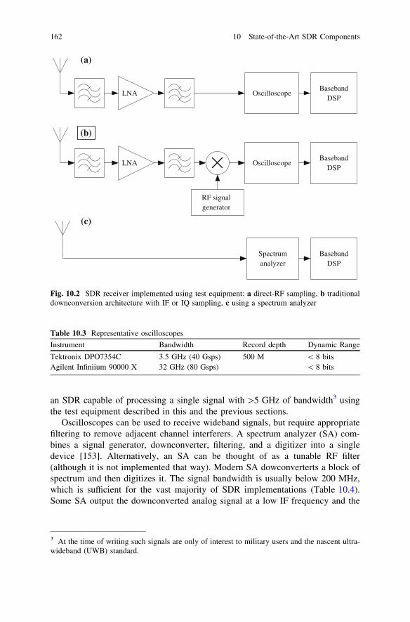
an SDR capable of processing a single signal with [5 GHz of bandwidth3 usingthe test equipment described in this and the previous sections.
Oscilloscopes can be used to receive wideband signals, but require appropriatefiltering to remove adjacent channel interferers. A spectrum analyzer (SA) com-bines a signal generator, downconverter, filtering, and a digitizer into a singledevice [153]. Alternatively, an SA can be thought of as a tunable RF filter(although it is not implemented that way). Modern SA dowconverterts a block ofspectrum and then digitizes it. The signal bandwidth is usually below 200 MHz,which is sufficient for the vast majority of SDR implementations (Table 10.4).Some SA output the downconverted analog signal at a low IF frequency and the
LNA OscilloscopeBaseband
DSP
LNA OscilloscopeBaseband
DSP
RF signalgenerator
Spectrumanalyzer
BasebandDSP
(a)
(b)
(c)
Fig. 10.2 SDR receiver implemented using test equipment: a direct-RF sampling, b traditionaldownconversion architecture with IF or IQ sampling, c using a spectrum analyzer
Table 10.3 Representative oscilloscopes
Instrument Bandwidth Record depth Dynamic Range
Tektronix DPO7354C 3.5 GHz (40 Gsps) 500 M \ 8 bitsAgilent Infiniium 90000 X 32 GHz (80 Gsps) \ 8 bits
3 At the time of writing such signals are only of interest to military users and the nascent ultra-wideband (UWB) standard.
162 10 State-of-the-Art SDR Components

digitized signal over a parallel digital interface (see Fig. 10.2c). These outputinterfaces are ideal for integration with the DSP subsystem to create a completeSDR.
10.1.3 Practical Considerations
The test equipment described in this section demonstrates state-of-the-art perfor-mance for RF carrier generation, baseband signal generation, and digitization. It isinteresting to consider whether a complete SDR can be developed using thisequipment and a separate (e.g. FPGA-based) DSP subsystem. The answer is‘sometimes.’
A combination of a vector signal generator (VSG) and a spectrum analyzer withappropriate digital baseband interfaces can be used to implement an SDR forsignal bandwidth below 200 MHz and carrier frequencies over a very wide range(Hz to GHz). For example, the Tektronix RSA6000 SA outputs the digitized IQdata over a 16-bit connector. Likewise, an Agilent E8267D can receive digital IQdata for upconversion over a similar interface. The DSP subsystem is thenresponsible for generating/processing digital samples in real time.
Higher bandwidth signals cannot be processed in real time using available testequipment. The wideband AWGs and oscilloscopes are designed to work on rel-atively short bursts of data. A pseudo-real-time wideband system with a low-dutycycle can be implemented. The transmitted samples are computed in the DSPsubsystem and transferred to the AWG (Fig. 10.3). The AWG is then triggered(e.g., based on absolute time) to transmit the burst of data. Likewise, an oscillo-scope can be triggered when the received signal level exceeds some threshold or ata specific time (Fig. 10.4). The digitized data is then transferred from the oscil-loscope and processed in the DSP subsystem. Oscilloscopes do not provide a wayto accurately time-tag the captured samples, but an additional device can be usedto record the time of each trigger. Clearly this solution is not suitable for a full-duplex TDMA links since the latency between transmission and reception is quitehigh (of the order of seconds).
It is theoretically possible to disassemble the wideband AWG and oscilloscopeand connect the internal DAC/ADC assembly directly to a DSP. Developing a DSPsubsystem capable of processing a signal with 10+ GHz bandwidth is extremelychallenging, but not impossible with today’s technology. Multiple FPGAs orASICs operating in parallel would be required to keep up with real-timeprocessing.
Table 10.4 Representative spectrum analyzers
Instrument Carrier Frequency Signal Bandwidth Dynamic Range
Agilent N9030A PXA 3 Hz to 50 GHz 140 MHz \ 14 bitsRohde-Schwartz FSQ 20 Hz to 40 GHz 120 MHz \ 14 bits
10.1 SDR Using Test Equipment 163

BasebandDSP
Clock AWGRF
signalgenerator
trigger
Ethernet IQ samplesTransmit time, T0
GPS
computesamples
transfersamples
setFc
setT0
Clock
PlayAWG &RF Gen
Fig. 10.3 Implementing a low-duty-cycle SDR transmitter using test equipment (dashed blocksare optional)
BasebandDSP
ScopeRF
signalgenerator
Clock
trigger
GPS
Carrier frequency IQ samples Receive time
Clock
Scope
recordtime
transfersamples
transfertime
processsamplesDSP
capture
Fig. 10.4 Implementing a low-duty-cycle SDR receiver using test equipment (dashed blocks areoptional)
164 10 State-of-the-Art SDR Components

10.2 SDR Using COTS Components
To make the leap from the laboratory to mass deployment, an SDR must becompetitive with single function radios in terms of cost, size, and power con-sumption. The high-end equipment described in the previous section definitelydoes not meet these requirements. This section examines components availableoff-the-shelf in high volumes and at reasonable cost.
10.2.1 Highly Integrated Solutions
Integration of multiple functional blocks on a single microchip is crucial to reducingcost and size of the solution. Some of the earliest work aimed at an integrated SDRRFFE was done at Interuniversity Microelectronics Centre (IMEC). Their latestiteration of a flexible RFFE, shown in Fig. 10.6, supports carrier frequencies from100 MHz to 3 GHz and signal bandwidth up to 20 MHz [154]. An entire book isdedicated to an earlier version of that chip [155]. Lime Microsystems offers themost flexible commercial RFFE on the market today. This single-chip transceiversupports carrier frequencies from 375 MHz to 4 GHz and signal bandwidth up to28 MHz [156]. A block diagram of this chip is shown in Fig. 10.5.
Note that both the IMEC and Lime chips use the direct-IF architecture describedin Sect. 6.2, and both integrate ADCs and DACs on the same chip. The two chips aremore similar than different, but the IMEC chip offers slightly better performance.
Fig. 10.5 Lime Microsystems flexible RFFE [156]
10.2 SDR Using COTS Components 165
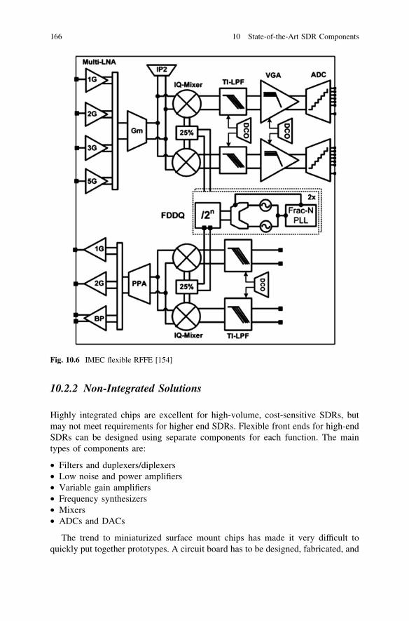
10.2.2 Non-Integrated Solutions
Highly integrated chips are excellent for high-volume, cost-sensitive SDRs, butmay not meet requirements for higher end SDRs. Flexible front ends for high-endSDRs can be designed using separate components for each function. The maintypes of components are:
• Filters and duplexers/diplexers• Low noise and power amplifiers• Variable gain amplifiers• Frequency synthesizers• Mixers• ADCs and DACs
The trend to miniaturized surface mount chips has made it very difficult toquickly put together prototypes. A circuit board has to be designed, fabricated, and
Fig. 10.6 IMEC flexible RFFE [154]
166 10 State-of-the-Art SDR Components

assembled just to put two chips together.4 RF components, on the other hand, comein both chip and connectorized versions (Fig. 10.7).
The author has met ‘old school’ RF designers from large military contractorswho were almost unaware of the ‘chip’ versions, and RF designers from startupsdeveloping cell phones who were completely unaware of the connectorized ver-sions. The two worlds seem to exist in parallel. Connectorized devices are pre-valent in very high frequency designs ([8 GHz) and are invaluable for quickprototyping. The connectorized versions are up to ten times more expensive andusually operate at higher voltages and burn more power. The connectorizeddevices are targeted at the high-end market and usually offer better performancethan bare chips.5 For example, a connectorized amplifier typically includesappropriate matching circuits.
10.2.3 Analog-to-Digital Converters (ADCs)
The dynamic range and bandwidth of an ADC converter is often the limiting factorin the flexibility of an SDR receiver.6 ADCs are semiconductor devices, but theirperformance does not follow Moore’s law—i.e., performance does not doubleevery 18 months. According to [35,157], the resolution-bandwidth7 productdoubles every 4 years and power consumption decreases by 50 % every 2 years.
Fig. 10.7 Connectorized and chip versions of RF components
4 Evaluation boards are sometimes available and can be used during the prototyping stage.5 There is, of course, nothing magical about the connectorized devices. Inside the box, they stilluse the chip components. However, the chips are attended by high-quality passives and the boardlayout is excellent.6 The ultimate limit for ADCs is estimated using the Heisenberg uncertainty principle. Using theequation DEDt [ h/2p, where DE is the energy of the smallest resolvable signal (� LSB), and Dtis half the sampling period (T/2), and h is Planck constant. Assuming a 1 V peak-to-peak inputsignal and a 50 X impedance, the Heisenberg limit yields 12 bits at 840 GS/s. This limit is *4orders of magnitude beyond the state-of-the-art which is currently aperture jitter limited [164].7 The number of bits quoted on ADC datasheets is an almost meaningless metric. The effectivenumber of bits (ENOB) is a better measure and is typically 2-5 bits less than the ‘nominal’resolution. ENOB is driven by a combination of noise and spurs.
10.2 SDR Using COTS Components 167
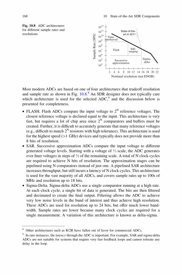
Most modern ADCs are based on one of four architectures that tradeoff resolutionand sample rate as shown in Fig. 10.8.8 An SDR designer does not typically carewhich architecture is used for the selected ADC,9 and the discussion below ispresented for completeness.
• FLASH. Flash ADCs compare the input voltage to 2N reference voltages. Theclosest reference voltage is declared equal to the input. This architecture is veryfast, but requires a lot of chip area since 2N comparators and buffers must becreated. Further, it is difficult to accurately generate that many reference voltages(e.g., difficult to match 2N resistors with high tolerance). This architecture is usedfor the highest speed ([1 GHz) devices and typically does not provide more than8 bits of resolution.
• SAR. Successive approximation ADCs compare the input voltage to differentgenerated voltage levels. Starting with a voltage of � scale, the ADC generatesever finer voltages in steps of � of the remaining scale. A total of N clock cyclesare required to achieve N bits of resolution. The approximation stages can bepipelined using N comparators instead of just one. A pipelined SAR architectureincreases throughput, but still incurs a latency of N clock cycles. This architectureis used for the vast majority of all ADCs, and covers sample rates up to 100s ofMHz and resolution up to 18 bits.
• Sigma-Delta. Sigma-delta ADCs use a single comparator running at a high rate.At each clock cycle, a single bit of data is generated. The bits are then filteredand decimated to create the final output. Filtering allows the ADC to achievevery low noise levels in the band of interest and thus achieve high resolution.These ADCs are used for resolution up to 24 bits, but offer much lower band-width. Sample rates are lower because many clock cycles are required for asingle measurement. A variation of this architecture is known as delta-sigma.
104
105
106
107
108
109
1010
1011
1012
2 4 8 10 12 14 16 18 20 22
Time-interleaved
Flash Sub-ranging
Successiveapproximation
Sigma-delta
State-of-the-art in 2011
Sam
ple
Rat
e [S
PS]
Nominal resolution (not ENOB)6
Fig. 10.8 ADC architecturesfor different sample rates andresolutions
8 Other architectures such as R/2R have fallen out of favor for commercial ADCs.9 In rare instances, the latency through the ADC is important. For example, SAR and sigma-deltaADCs are not suitable for systems that require very fast feedback loops and cannot tolerate anydelay in the loop.
168 10 State-of-the-Art SDR Components

• Time Interleaved. Time interleaved ADCs apply the concept of parallel processingby using multiple ADCs simultaneously. The sample time for each constituentADC is offset relative to others by either delaying the sample clock or the inputsignal. For example, 10 ADCs sampling at 10 MHz and offset in time by 10 ns are‘equivalent’ to a single ADC sampling at 100 MHz. This architecture is only used
Fig. 10.9 Published ADC performance (1993-2011): bandwidth versus precision (line indicatesperformance limit for sample jitter of 1 ps) [158]
Fig. 10.10 Published ADC performance (1993-2011): power consumption versus precision(line indicates 10 pJ/fs) [158]
10.2 SDR Using COTS Components 169
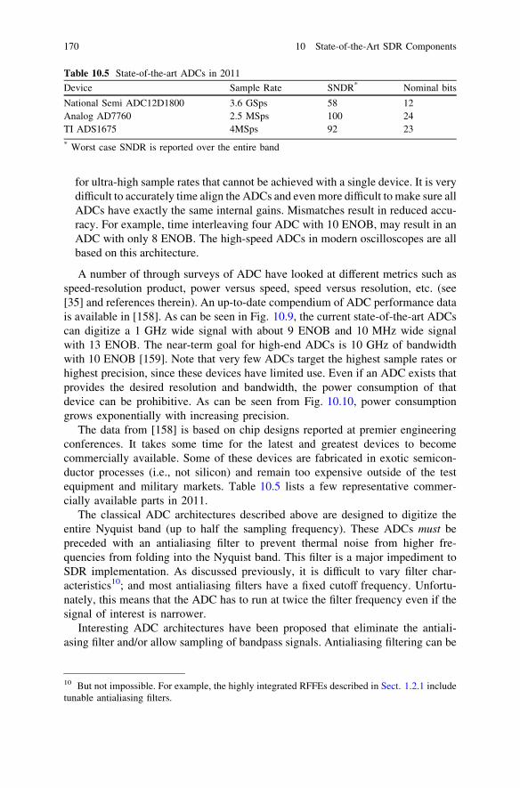
for ultra-high sample rates that cannot be achieved with a single device. It is verydifficult to accurately time align the ADCs and even more difficult to make sure allADCs have exactly the same internal gains. Mismatches result in reduced accu-racy. For example, time interleaving four ADC with 10 ENOB, may result in anADC with only 8 ENOB. The high-speed ADCs in modern oscilloscopes are allbased on this architecture.
A number of through surveys of ADC have looked at different metrics such asspeed-resolution product, power versus speed, speed versus resolution, etc. (see[35] and references therein). An up-to-date compendium of ADC performance datais available in [158]. As can be seen in Fig. 10.9, the current state-of-the-art ADCscan digitize a 1 GHz wide signal with about 9 ENOB and 10 MHz wide signalwith 13 ENOB. The near-term goal for high-end ADCs is 10 GHz of bandwidthwith 10 ENOB [159]. Note that very few ADCs target the highest sample rates orhighest precision, since these devices have limited use. Even if an ADC exists thatprovides the desired resolution and bandwidth, the power consumption of thatdevice can be prohibitive. As can be seen from Fig. 10.10, power consumptiongrows exponentially with increasing precision.
The data from [158] is based on chip designs reported at premier engineeringconferences. It takes some time for the latest and greatest devices to becomecommercially available. Some of these devices are fabricated in exotic semicon-ductor processes (i.e., not silicon) and remain too expensive outside of the testequipment and military markets. Table 10.5 lists a few representative commer-cially available parts in 2011.
The classical ADC architectures described above are designed to digitize theentire Nyquist band (up to half the sampling frequency). These ADCs must bepreceded with an antialiasing filter to prevent thermal noise from higher fre-quencies from folding into the Nyquist band. This filter is a major impediment toSDR implementation. As discussed previously, it is difficult to vary filter char-acteristics10; and most antialiasing filters have a fixed cutoff frequency. Unfortu-nately, this means that the ADC has to run at twice the filter frequency even if thesignal of interest is narrower.
Interesting ADC architectures have been proposed that eliminate the antiali-asing filter and/or allow sampling of bandpass signals. Antialiasing filtering can be
Table 10.5 State-of-the-art ADCs in 2011
Device Sample Rate SNDR* Nominal bits
National Semi ADC12D1800 3.6 GSps 58 12Analog AD7760 2.5 MSps 100 24TI ADS1675 4MSps 92 23* Worst case SNDR is reported over the entire band
10 But not impossible. For example, the highly integrated RFFEs described in Sect. 1.2.1 includetunable antialiasing filters.
170 10 State-of-the-Art SDR Components

integrated into the digitization process as described in [160]. Removing the an-tialiasing filter is very desirable for SDR implementations. The sigma-deltaarchitecture can be adapted to digitize a narrowband signal centered at a non-zerocarrier frequency as described in [161]. A number of the bandpass sampling ADCshave been reported in the last 10 years. However, they have limited applicabilityto SDR since the signal center frequency is not easily tunable.
10.2.4 Digital to Analog Converters (DACs)
DACs do not receive nearly as much attention in the research community asADCs.11 DACs are arguably easier to implement than ADCs. Interestingly, DACarchitectures closely mirror those of ADCs:
• A fully parallel implementation uses either 2N resistors or current sources. Thisarchitecture provides the highest sample rate. However, matching the individualsources becomes very difficult, limiting the precision of the DAC.
• Binary weight. These DACs use N resistors or current sources, with each sourceweighted according to its position in the N-bit word.
• Sigma-Delta. This architecture is very similar to the ADC sigma-delta.• Hybrid architectures. Most practical DACs use a combination of the above
architectures. For example, the MSBs may be implemented full parallel, and theLSBs using the binary weights.
Table 10.6 lists a few representative commercially available parts in 2011(Fig. 10.11).
10.3 Exotic SDR Components
The test equipment and COTS components described in the previous two sectionsare available (at a price) to most SDR developers. This section briefly touches onsome new and exotic technologies that have not yet made it out of the lab. Some of
Table 10.6 State-of-the-art DACs in 2011
Device Sample Rate SFDR* Quoted resolution
Euvis MD662H 8 GSps 45 12Maxim MAX5881 4.3 GSps 60 12TI DAC5670 2.4 GSps 60 14Maxim MAX5895 500 MSps 73 16Analog AD9122 1.2 GSps 72 16
11 An informal search of the IEEEXplore database for the past 10 years returned *4,000 paperson ADCs and *1,000 papers on DACs.
10.2 SDR Using COTS Components 171

the most interesting research on very wideband data conversion involves the use ofphotonic components [163]. A comprehensive overview of ADC technology ingeneral and photonic ADCs in particular is provided in [164]. In a genericphotonic ADC, the electrical signal that must be digitized is first modulated onto alaser beam. The laser beam is then processed in the optical domain using nonlinearoptical components. The processed optical signal(s) are then converted back to theelectrical signals using photodetectors. The electrical signals are finally processedusing standard electronic ADCs/DACs. The resultant system is not yet practical forcommercial SDRs. Optical components are currently quite large (but gettingsmaller [165]) and expensive. The power consumption of the laser source can bequite high. Photonic ADCs currently provide very wide bandwidth (*80 GHz)but limited resolution (\4 bits).
Photonic components are also being applied to the RFFE chain [166]. Photoniccirculators [167] and tunable filters (see Sect. 1.4) have been reported in the openliterature. These exciting developments are mainly of interest to the academic andmilitary communities but will most likely trickle down to the commercial SDRdevelopers in the coming years.
Cryogenics has been used in the design of high-end radios for many years.Improvements in cryo-cooler design are making these components more accessi-ble. Cryo-ADCs offer both lower power consumption12 and higher resolutionbandwidth products than room temperature ones [168]. At least one company isaggressively marketing a cryo-ADC [169] based on a sigma-delta architecture.
35
40
45
50
55
60
65
70
75
80
1E+02 1E+03 1E+04
SFD
R
Sample Rate [MSps]
Fig. 10.11 Published DAC performance specifications (1995-2010) [162]
12 Neglecting the power consumption of the cryogenic subsystem.
172 10 State-of-the-Art SDR Components

According to the marketing materials from HYPRESS, their digital-RF receiver isvery close to an ideal SDR. However, a tunable channel select filter is still requiredfor the RFFE.
One particularly interesting system combines photonics and cryogenics.Measuring the power spectrum density (PSD) over a wide bandwidth and doing itquickly is very important for cognitive radio (see Sect. 3.4). The traditionalapproach uses a wideband ADC to digitize the samples, and then a high-speed FFTengine on a GPP or FPGA to compute the PSD. A few GHz of spectrum can beanalyzed using state-of-the-art ADCs. A photonic spectrum analyzer relies on aunique property of a Thulium-doped YAG crystal cooled down to 5�K [170, 171].This crystal can ‘record’ PSD of a microwave signal with well over 10 GHz ofbandwidth (extendable to 200 GHz using a different crystal [172]). A stable laseris modulated with the received microwave signal. The modulated laser passesthrough the crystal and ‘burns in’ the PSD. The recorded PSD is then read out witha narrowband chirped laser and digitized at a rate of up to 1,000 Hz. Note that theADC need not be particularly fast—100 MHz is sufficient. Thus, a complete10+ GHz spectrum can be measured every ms with about 60 dB of dynamic range.This ultra-exotic and very expensive ($200 k +) technology is aimed squarely atthe military market (Fig. 10.12). As is often the case, the answer to a question‘‘what is possible in today’s technology?’’ is that it depends on how much moneyis available.
10.4 Tunable Filters
Lack of a tunable RF bandpass filter is the single largest impediment to realizationof an ideal SDR receiver. Tunable filters are also desirable, but are not required forSDR transmitters. This section briefly covers existing and emerging technologiesfor tunable RF filters. A key metric for a filter is its Q factor—the ratio of thebandwidth to the center frequency (Fig. 10.13). The higher the Q, the narrower and‘‘sharper’’ the filter. For example, to extract a 1 MHz signal at a carrier frequency
Stablelaser
Optical modulator
Tm:YAGcrystal
Readoutchirp laser
Photo-detector
A/D
Cryo cooler
Fig. 10.12 Ultra-wideband photonic/cryogenic spectrum analyzer
10.3 Exotic SDR Components 173

of 1 GHz, the Q should be approximately 1,000. It turns out that designing filterswith large Q is difficult. Both the center frequency and the bandwidth of a tunablefilter should be continuously and independently variable. An excellent review oftunable filters is available [173].
The main technologies for manufacturing RF filters are:
• RLC (Fig. 10.14a). RLC filters are designed using standard resistors (R),capacitors (C), and inductors (L). These devices can be discrete parts mountedon a substrate (for lower Fc) or traces on a circuit board (for higher Fc). It isdifficult to get high Q-factors with RLC filters because many stages of filteringare required. RLC values in each stage must be closely matched to achieve the
0
BW
Fc
BWFc=Q
Frequencyrolloff
Fig. 10.13 Filter Q factor
Fig. 10.14 Sample filters a RLC, b SAW, c waveguide
174 10 State-of-the-Art SDR Components

desired frequency response. RLC filters can be tuned by changing the value ofone or more components (usually the capacitor).
• SAW (Fig. 10.14b). Surface acoustic wave filters are mechanical (not elec-tronic) devices that happen to resonate at some frequencies and dampen others.SAW filters have very high Q-factors and very sharp rolloff. Unfortunately, theydo not work well above 3 GHz and are not tunable.
• Waveguide (Fig. 10.14c). Waveguide (and cavity) filters rely on constructiveand destructive interference of EM waves in the filter cavities to achieve thedesired response. These filters are typically machined out of single block ofmetal. The filter size is inversely proportional to the center frequency. Wave-guide filters are mostly used for frequencies above 2 GHz since they are verylarge for lower frequencies. Waveguide filters can be tuned by changing thedimensions of the cavities (e.g., by tightening or loosening strategically placedscrews).
Selecting one from a bank of available filters is currently the most populartechnique to create a tunable filter (Fig. 10.15). The constituent filters can use anytechnology. The disadvantages of this approach are clear:
• Multiple filters take up a lot of space.• Each level of switching causes loss of signal power (less than 0.5 dB per stage),
reducing receiver SNR or increasing transmitter power requirements.• The switches are not ideal, and large interferers can leak into the signal of
interest through the ‘off’ switches.• The filter is only minimally tunable—bandwidth cannot be changed, and only a
few center frequencies are available.
Mechanically tunable filters have been available for decades. In fact, somehigh-end analog AM/FM radio receivers used tunable filters. Turning the tuningdial actually moved capacitor plates in and out, changing the center frequency ofan RLC filter.13 The center frequency of these filters can be varied contiguouslyover the filter range (typically one octave). However, the Q factor is fixed and thefilter bandwidth increases at higher center frequencies. These filters are valuablefor laboratory use but are of limited practical use for SDR development(Fig. 10.16).
RFFE
Fig. 10.15 Tunable filterusing a filter bank
13 Most radios just used that variable capacitor to change the output frequency of the synthesizer.
10.4 Tunable Filters 175

Tunable RLC filters are created by using devices with variable capacitance. Twomain technologies for electrically (vs. mechanically) tunable capacitance are var-actors and ferroelectric films. The dielectric constant of a ferroelectric compoundBST (barium strontium titanate) changes with applied voltage. BST can therefore beused to make variable capacitors [175]. At least one company is attempting tocommercialize BST technology [176].14 BST-based tunable filters have beenreported for a wide range of center frequencies, from baseband to 30 GHz [177, 178]with high Q-factors. Unfortunately, BST filters require large voltages to tune—up to100 V. To the best of the author’s knowledge, BST filters are not commerciallyavailable. Varactors are simply diodes fabricated in standard semiconductor pro-cesses. They are inexpensive and easily integrated on the same die as other RF andmixed-signal circuits. Varactor-based tunable filters are used in the single-chipRFFE described in Sect. 1.2.1. Unfortunately, these filters cannot achieve highQ-factors and are not readily usable for carrier frequencies above 500 MHz. Arepresentative example of a varactor-tuned filter is marketed by Hittite [179].
Yttrium-Iron-Garnet (YIG) is a ferromagnetic material that has been used tomake tunable filters since the 1960s. A magnetic field is used to change filterproperties. Unlike the mechanically tunable filters described above, the bandwidthof a YIG filter is typically fixed (and typically \100 MHz) and does not changewith the center frequency. YIG filters have been reported that cover center fre-quencies from 0.5 to 40 GHz [180]. The passband of these filters is not very flatand requires equalization in the DSP subsystem. YIG filters consume a lot ofpower to generate the required magnetic field. They are also quite large (typicallyabout 10 cm3), and therefore not suitable for use in handheld devices. They cannothandle power above 10 dBm, and are therefore not suitable for filtering poweramplifier output in a transmitter. Despite their drawbacks, YIG filters are currentlythe only solution for truly wideband and high-Q filters. A number of vendors are
Fig. 10.16 Mechanically tunable filters: a manual control, b electronic control [174]
14 The filters marketed by AgileRF are targeted for baseband antialiasing rather than for RFchannel selection.
176 10 State-of-the-Art SDR Components

actively marketing YIG filters [181,182,183], targeting the high-end communi-cations and military markets. Performance of a representative filter is shown inFig. 10.17. Note the very high Q and a significant ripple in the passband.
The most promising technology for high-Q wideband tunable RF filters ismicro-electro-mechanical-systems (MEMS). MEMS-based RF filters use a largenumber of miniature on/off switches to add and remove capacitors from the circuit[184]. The resistance of each switch is very small, making the overall insertion losssmall. A MEMS filter can be thought of as a highly miniaturized version of thefilter in Fig. 10.15. Most MEMS filters are not truly continuously tunable, sincethe number of bandwidth and center frequencies is determined by the numberof switches. However, if the tuning resolution (inversely proportional tolog2(#switches)) is reasonably high ([5 bits), the filter can be consideredcontinuously tunable for all practical purposes. MEMS filters can be integratedinto a standard semiconductor process, making them potentially low cost, verycompact, and low power. Design of these filters is currently a very active researcharea with over 1,000 papers published in the last 10 years. However, to the best ofthe author’s knowledge, they are not yet commercially available. Transistor-basedswitches can be used instead of MEMS switches, but offer lower performance.
The technologies described in this section are summarized in Table 10.7.RF photonics filters rely on nonlinear properties of optical components. These
filters first modulate the RF signal on an optical carrier (i.e., laser) and process thelaser beam in the optical domain before converting back to electrical. Just like thephotonic ADCs described earlier, photonic RF filters have not yet made it out ofthe laboratory. However, some very exciting development is taking place withchip-scale photonics [185,186]. Photonic components are being integrated on asemiconductor chip, making the entire filter relatively compact and low cost. Thefilters reported so far offer very a wide range of center frequencies, but do notallow narrow bandwidth. The most impressive photonic filter, reported in [187],offers a center frequency of 1–40 GHz and a bandwidth of 250–1,000 MHz. Theseresults are significantly better than prior art and should be treated as ‘what will be
Fig. 10.17 RepresentativeYIG filter tuned over 1–2 GHz range
10.4 Tunable Filters 177
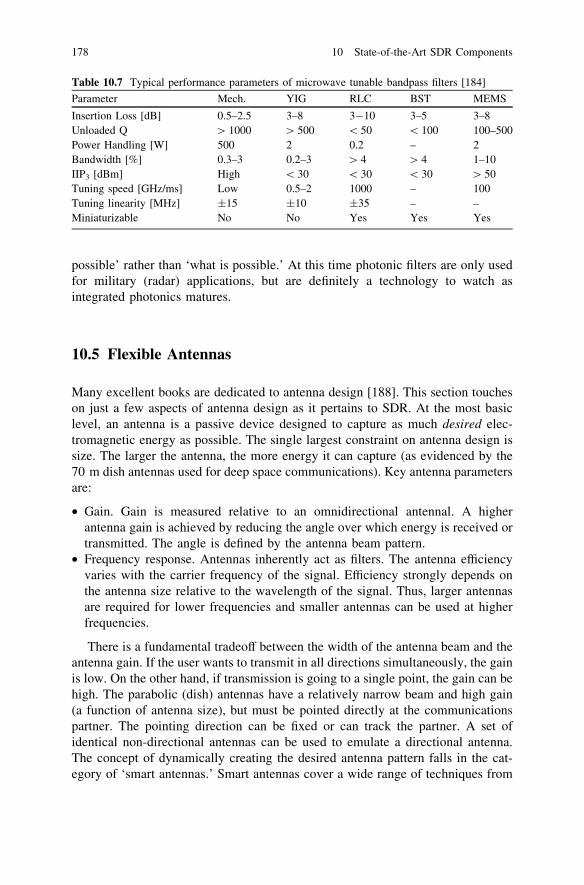
possible’ rather than ‘what is possible.’ At this time photonic filters are only usedfor military (radar) applications, but are definitely a technology to watch asintegrated photonics matures.
10.5 Flexible Antennas
Many excellent books are dedicated to antenna design [188]. This section toucheson just a few aspects of antenna design as it pertains to SDR. At the most basiclevel, an antenna is a passive device designed to capture as much desired elec-tromagnetic energy as possible. The single largest constraint on antenna design issize. The larger the antenna, the more energy it can capture (as evidenced by the70 m dish antennas used for deep space communications). Key antenna parametersare:
• Gain. Gain is measured relative to an omnidirectional antennal. A higherantenna gain is achieved by reducing the angle over which energy is received ortransmitted. The angle is defined by the antenna beam pattern.
• Frequency response. Antennas inherently act as filters. The antenna efficiencyvaries with the carrier frequency of the signal. Efficiency strongly depends onthe antenna size relative to the wavelength of the signal. Thus, larger antennasare required for lower frequencies and smaller antennas can be used at higherfrequencies.
There is a fundamental tradeoff between the width of the antenna beam and theantenna gain. If the user wants to transmit in all directions simultaneously, the gainis low. On the other hand, if transmission is going to a single point, the gain can behigh. The parabolic (dish) antennas have a relatively narrow beam and high gain(a function of antenna size), but must be pointed directly at the communicationspartner. The pointing direction can be fixed or can track the partner. A set ofidentical non-directional antennas can be used to emulate a directional antenna.The concept of dynamically creating the desired antenna pattern falls in the cat-egory of ‘smart antennas.’ Smart antennas cover a wide range of techniques from
Table 10.7 Typical performance parameters of microwave tunable bandpass filters [184]
Parameter Mech. YIG RLC BST MEMS
Insertion Loss [dB] 0.5–2.5 3–8 3-10 3–5 3–8Unloaded Q [ 1000 [ 500 \ 50 \ 100 100–500Power Handling [W] 500 2 0.2 – 2Bandwidth [%] 0.3–3 0.2–3 [ 4 [ 4 1–10IIP3 [dBm] High \ 30 \ 30 \ 30 [ 50Tuning speed [GHz/ms] Low 0.5–2 1000 – 100Tuning linearity [MHz] ±15 ±10 ±35 – –Miniaturizable No No Yes Yes Yes
178 10 State-of-the-Art SDR Components

MIMO (see Sect. A.6) to beamforming. Beamforming is a technique that com-bines appropriately scaled and delayed signals to (from) individual antennas tocreate the desired beam shape. A beam can be shaped to send all energy to thepartner(s), or to avoid (null) an interferer, or achieve a combination of these goals(Fig. 10.18). SDR is an excellent platform for implementing smart antenna tech-niques. The algorithms are implemented entirely in the DSP subsystem and willnot be discussed here.
The relationship between antenna dimensions and its frequency response is oneof the biggest hurdles in implementing a wideband SDR. Physics tells us that alarge antenna is required to receive low frequency signals. For example, if an SDRneeds to process carrier frequencies down to 100 MHz, the antenna size must be ofthe order of 1 meter. Smaller antennas will work, but result in reduced SNR. Thereare two approaches to supporting a wide range of frequencies for an SDR antenna:
1. Use a wideband antenna that provides reasonable performance over the entireband.
2. Use a tunable antenna that provides good performance over a narrow band, butallows the band to be tuned over a wide range.
Neither approach is better than the other in all cases. For example, a cognitiveradio that must monitor spectrum looking for available bandwidth needs to have awideband antenna. On the other hand, once a band is selected, a tunable antennasimplifies filtering requirements. A tunable narrowband antenna typically provideshigher gain than a similarly sized wideband antenna.
The basic idea behind most tunable15 antennas is to selectively add and removesegments to achieve the desired geometry, or add capacitors and inductors toachieve the desired resonance frequency. Segments can be added by closingswitches between them. The switches can be made using either MEMS [189,190]or semiconductor devices [191] (Fig. 10.19). Tunable antennas are not yet com-mercially available. A mechanically tunable antenna that uses micropistons insteadof MEMS switches was developed by Synotics and is reported in [192].
An entirely different type of antenna has recently been resurrected fromobscurity. A plasma antenna uses highly ionized air instead of metal to interactwith electromagnetic waves. The size of the ionized volume can be varied by
User 1
User 2
InterfererDSP
AntennasRFFEsFig. 10.18 Application ofsmart antenna technique(beamforming)
15 Matching the antenna impedance to the RFFE circuits is a separate task.
10.5 Flexible Antennas 179

changing the applied voltage (or magnetic field). Plasma antennas are thereforeinherently tunable. A comprehensive review is provided in [193] and [194].Despite their somewhat exotic origins,16 plasma antennas can be implemented insilicon for low cost and size. At least one company is actively pursuing com-mercialization of plasma antennas [195].
Since tunable antennas are not yet commercially available, a wideband antennais the next best thing for an SDR. Fortunately, many wideband antennas areavailable—from compact designs suitable for handheld devices to large YAGIs.A representative wideband antenna and its VSWR are shown in Fig. 10.20. Note
Frequency [GHz]
VSW
R
2 3 4 5 6 7 81
2
3
4
5penny
Fig. 10.20 Representativewideband (2-8 GHz)antenna
Fig. 10.19 Using MEMS switches to configure antenna geometry [189]: a elements andswitches, b top view of a switch, c side view of a closed switch, d side view of an open switch
16 Plasma antennas are of significant interest to the military because they ‘disappear’ andbecome invisible when plasma generation is de-energized [272].
180 10 State-of-the-Art SDR Components

that VSWR increases (efficiency decreases) at lower frequencies because theantenna is small (just under � wavelength at 2 GHz). Another relatively compactantenna that covers 0.4–18 GHz is described in [196] and shown in Fig. 10.21.Large antennas that cover frequencies from 100 MHz to 40 GHz are available.Interesting spiral antennas developed specifically for SDR are reported in [197].
60 cm
Frequency [GHz]
Gai
n [d
Bi]
10
5
0
0.5 108642
Fig. 10.21 Very wideband antenna (log-periodic) [196]
10.5 Flexible Antennas 181

Chapter 11Development Tools and Flows
Tools used to develop SDR are equally applicable to single-function radios and othercomplex systems with extensive DSP requirements. The required toolset and devel-opment flow strongly depends on the hardware architecture. Unique tools are requiredfor FPGA, ASIC, or DSP implementations. Few decisions engender as much passionas the choice of tools and languages for a new development. Many developers feelalmost religious attachment toward their language of choice (C++ vs. Java, Verilog vs.VHDL). In the author’s opinion, the choice of a tool within the same class (e.g. C++ vs.Java) makes only a small difference, and the expertise of the key team members countsfor a lot. However, switching between classes of tools (e.g. VHDL vs. MATLAB/Simulink) can make a dramatic difference (though not always the expected one).
A highly simplified flowgraph for a typical SDR development process is shownin Fig. 11.1. This flowgraph does not capture any of the optimization/iterationloops that are invariably required in the course of development.1
The requirements defined in the first step are used to drive architecture selec-tion. Different SDR architectures (e.g. FPGA, GPP, etc.) are discussed in Chap. 5.The choice of architecture determines which branch(es) in Fig. 11.1 will be taken.
11.1 Requirements Capture
Requirements definition is without a doubt the most important step in SDR devel-opment. As discussed in Sect. 4.2, constraining the capabilities of a SDR is non-trivial. Many SDR requirements mirror those for single function radios but with listsprovided for each option (e.g. ‘‘radio shall support modulations: QPSK, 16QAM;data rates: 0.5–10 Mbps’’, etc.). Unfortunately, these types of requirements oftenlead to poorly designed SDRs. The final product does in fact support all the options,but may not be flexible enough to support minor variations. For example, to ensure
1 Ideally, the loops only go between adjacent levels. In practice, it is not unreasonable for anintractable problem encountered at the implementation of the ASIC physical layer to affect therequirements, causing a ripple of changes down the flowgraph.
E. Grayver, Implementing Software Defined Radio,DOI: 10.1007/978-1-4419-9332-8_11, � Springer Science+Business Media New York 2013
183

flexibility, the modulation requirement is better stated as: ‘‘radio shall support anarbitrary constellation described by 2, 4, 8, or 16 points in the complex plane.’’ Themore general requirement ensures that the radio can support a 12/4 APSK modula-tion, which is slightly different from 16-QAM.
In general, many SDR requirements should read ‘‘shall be capable of supportingX…’’ rather than ‘‘shall support X…’’ For the first clause, the developer mustestimate required hardware to support X. For the latter clause, the developer mustactually implement X and it is unreasonable to implement all possible waveformsan SDR can support. Of course, these requirements are more difficult to verify. Awell-planned SDR development should include a minimum set of waveforms andfeatures at launch, and anticipate new waveforms to be added in the future. Thus,the developer can select an architecture that can readily accommodate the plannedfeatures, without requiring that those features be implemented immediately.
The amount of formality and paperwork in the requirements definition phasevaries dramatically. A SDR intended for laboratory R&D has few true require-ments and a large number of desirements. On the other hand, a SDR meant formilitary field use must comply with a draconian requirements capture process.2
Requirements Definition
Requirements Flowdown
Architecture Specification
System Simulation
FirmwareDevelopment
Implementation
Physical Layer
SoftwareDevelopment
PerformanceOptimization
Hardware/RFDevelopment
Mechanical
Verification
Fig. 11.1 Simplified SDR development flowgraph
2 A nice set of ‘‘requirements for requirements’’ is articulated in [273]:Correct (technically and legally possible); Complete (express a whole idea or statement); Clear
(unambiguous and not confusing); Consistent (not in conflict with other requirements); Verifiable(it can be determined that the system meets the requirement); Traceable (uniquely identified andtracked); Feasible (can be accomplished within cost and schedule); Modular (can be changedwithout excessive impact); Design-independent (do not pose specific solutions on design).
184 11 Development Tools and Flows

A dedicated software tool is recommended for all but the most relaxedrequirements capture processes (a word processor is not an appropriate tool).These tools range from the high-end, such as IBM Rational DOORS [198], to theopen source OSRMT [199]. Many of these tools support a graphical languageknown as the Unified Modeling Language (UML) [200]. UML provides graphicalnotation techniques to describe how the system should operate, which can then betranslated into actionable requirements. For example, UML can be used to describedifferent use cases, event sequence diagrams, or relationships between blocks inthe system.
The requirements flowdown process takes the high-level requirements andbreaks them down into actionable sub-requirements. For example, a requirement‘‘the transmitter shall support symbol rates up to 100 MSps’’ can be broken intothe following sub-requirements, and each sub-requirement must be traceable to theparent requirement.
1. The DAC shall support sample rate of at least 200 MSps2. The power amplifier shall have a bandwidth of at least 150 MHz3. The DSP subsystem shall support a contiguous sample rate of at least
200 MSps.
Each sub-requirement should be linked to a software or firmware file thatimplements the code to satisfy the requirement. High quality requirements capturetools allow dynamic linking between the source code and the requirement.
Fig. 11.2 Representing a QPSK modulator with pulse shaping. a Simulink. b Systemvue.c MATLAB
11.1 Requirements Capture 185

11.2 System Simulation
System level simulations allow rapid development of models or prototypes for theentire system or selected critical components. This allows developers to plan andtest the big-picture architectures, features, and design parameters before focusingprematurely on final implementation details. System level simulations should beused to verify the performance of selected algorithms under a wide range ofexpected conditions. For example, signal acquisition would be tested for worst-case frequency and timing offsets and worst-case SNR.
System simulation tools fall into two categories (Fig. 11.2):
1. Code-based tools require the developer to describe the algorithms as a set ofsequential commands in a specific language. A simulation may be written inMATLAB, C++, Python, etc. MATLAB is currently the tool of choice for themajority of DSP engineers because of the vast library of predefined functions(toolboxes).3
2. Block-based tools require the developer to draw block diagrams to describe thealgorithms. Popular block-based tools used today include Simulink, SignalProcessing Workbench (SPW), and SystemVue. Simulink is by far the mostwidely used. Each tool comes with a library of predefined blocks (corre-sponding to predefined functions for code-based tools). The richness of theblockset is a key differentiator between tools. Additional blocks can be createdby either combining existing blocks (hierarchical design), developing newblocks in a code-based tool (e.g. C++) with appropriate wrappers, or purchasinglibraries from third-party vendors.
One fundamental difference between code and block tools is the way dataflowis handled. Code-based tools expect the developer to manage data transfer betweenfunctions. Block-based tools implicitly provide buffers and flow control betweenblocks. The difference is apparent in long simulations. A simulation in a code-based tool cannot allocate enough memory4 to hold all of the data required for thesimulation at once. The developer must therefore create a loop to break up the longsimulation into smaller chunks. Preserving the internal state for all the functionsbetween each chunk is messy and error-prone. On the other hand, a block-based
3 Interestingly, some developers targeting ASICs strongly prefer C++ for system simulation.This preference may be due to higher simulation speeds offered by C++ versus MATLAB. AnASIC design must be very thoroughly tested across every possible scenario since it cannot bechanged after fabrication. The additional effort required to write simulations in C++ is justified byreduced runtimes.4 The author came across one project where the system analysts kept requesting more and moreRAM for their computers. At one point, a simulation was taking 16 GB and was running veryslowly. A quick look at their code revealed that the entire simulation was processed in one step.Eventually the simulations got too long for even high-end machines and the code had to berewritten to break up the simulation into smaller chunks. The updated code required less than1 GB of RAM and ran twice as fast.
186 11 Development Tools and Flows

simulation can process an arbitrary amount of data because each block implicitlysaves its own state. If a block-based simulation processes samples one at a time,the simulation cannot take advantage of modern microprocessors’ vector com-putation units and runs slowly. Thus, modern block-based simulations introduce aconcept of ‘frames’ to process data in small chunks. Simulations execute muchfaster5 (but still slower than code-based) but become somewhat more difficult tomanage if the underlying algorithms require feedback loops that operate onsamples.
Despite slower performance, block-based simulators are becoming more andmore popular. Proponents argue that a block diagram is easier to understand thanequivalent function calls. The simulator framework takes care of many details,making designers more productive. Perhaps the strongest argument for block-based simulations is the newly emerging option to transition a model intoimplementation (discussed below).
Simulink is the most general purpose of the commercially available block-based simulators. It is also one of the newest entrants into the marketplace.However, tight integration with the immensely popular MATLAB has madeSimulink a clear leader.
Signal processing workstation (SPW) is one of the oldest system simulationtools. It was very popular in the 1990s, and is still used by defense contractors withlarge libraries of legacy designs. In the past decade, SPW has changed hands fromCadence to CoWare to Synopsys. It remains an extremely powerful tool withbetter visualization and interaction features than Simulink. SPW was probably thefirst tool to offer a path from simulation to hardware implementation. The libraryof blocks offered by SPW is unsurpassed by any competitors (SystemVue is a closesecond) and includes complete solutions for many modern wireless standards.However, SPW costs over ten times more than Simulink, making it accessible onlyto deep-pocketed companies. More importantly, momentum is definitely withSimulink.
SystemVue is an interesting tool that is arguably easier to use than Simulink. Itis targeted specifically for communications system design and has a rich set ofcommunications-specific blocks. Its main strength is a clean interface betweendigital baseband and RF components. It is the only tool to include a comprehensiveset of distortion parameters for fundamental analog blocks (e.g. differential non-linearity properties of a DAC). SystemVue is also unique in that it offers tightintegration with Agilent test equipment (e.g. simulation output can be sent directlyto a signal generator and the visualization interface is identical to that of a vectorsignal analyzer). The same GUIs can therefore be used for the entire developmentprocess from system simulation to hardware debugging.
5 The author compared throughput of a simulation of a simple BPSK modem with pulse shapingcoded using optimized C++, MATLAB, and Simulink. The relative throughput was 13:6:1.Throughput of frame based vs. sample based Simulink simulation was 3:1.
11.2 System Simulation 187

The three products described above are by no means the only available block-based system simulation tools. Tools like VisSim and LabView have a small shareof the system simulation pie. In fact, even the GNURadio/GRC platform describedin Sect. 8.1 can be used for simulations.
Firmware and software development starts after system simulations are com-plete and results satisfy the requirements.
11.3 Firmware Development
For the purposes of this section, ‘firmware’ refers to code intended for imple-mentation on an FPGA or ASIC.
The standard practice in the past was for a systems engineer to hand off a set ofrequirements, algorithm documentation, and system models to a hardware engi-neer. The hardware engineer then translated the (usually) MATLAB code to ahardware description language (HDL, VHDL or Verilog). The hardware engineerwas responsible for mapping the algorithm to available hardware resources (logicgates, multipliers, memory, etc.) while meeting throughput and latency require-ments. The system model generated necessary stimulus files and output files foreach algorithm. The hand-coded HDL was then simulated with the stimulus fileand the output was compared to the ‘golden’ output from the system model. Thisprocess was time consuming and error-prone. The hardware engineer did notdevelop the algorithm, making it difficult for him to debug problems. The systemengineer is usually not well versed in the hardware ‘costs’ of different algorithmsand can easily come up with a solution that is very inefficient in terms of hard-ware.6 Many time-consuming iterations are frequently required to converge on afunctional implementation of a hardware-efficient algorithm (Fig. 11.3). The nexttwo subsections present some recent developments that promise to reduce devel-opment time by allowing design at a higher level of abstraction.
11.3.1 Electronic System Level Design
Designs are getting more and more complex, but the chip resources available todesigners increase even faster. There is a strong effort in industry to combine theroles of system and hardware engineers. This effort is centered on a concept calledelectronic system level (ESL7) design [201, 202]. The goal is to develop firmware
6 A division operator (7) does not typically warrant a second thought from a communicationsengineer, but dividers are anathema to hardware designers because they are difficult to implementand require a lot of resources.7 Also known as high-level synthesis (HLS).
188 11 Development Tools and Flows

at the system level, bypassing the manual conversion of the system model to HDL.The idea is by no means new—a tool called Behavioral Compiler was marketed bySynopsys as early as 1994 [203] (also see [204] for a comprehensive but somewhatbiased history). Unfortunately, the tools were not good enough, and chip resourceswere too valuable to waste on poorly optimized designs. ESL got a second windaround 2005 with the introduction of a few tools that promised to convert standard(or semi-standard) ‘C’ code to HDL. Some of the entrants were: Impulse-C, Dime-C, Handel-C, and the only currently surviving option, SystemC. SystemC has yetto be widely adopted and may follow the fate of the others. An extremelypromising tool was developed by AccelChip to convert MATLAB code directly toHDL. Unfortunately this tool never gained enough traction, and was discontinuedby 2009. It appears that high level synthesis is still ‘‘almost there’’ after 15 years.A recent article [205] highlights the primary difficulty of HLS––the same algo-rithm can be implemented using very different hardware architectures with easily10009 difference in design size and performance between them.
If we are expecting C-to-FPGA to ever behave like a software compiler, we’re over-looking an important fact about the difference between hardware and software. For asoftware compiler, there is always something that could be agreed upon as a ‘‘best’’solution. Compiler developers can tune away—trying to minimize the size and maximizethe speed of the generated code. The right answer is reasonably easy to quantify. Opti-mization choices made during software compilation have at best a modest effect on theresults. For the sake of argument, maybe zero to 20 % plus or minus.8
Firmware
System simulation
StimulusGoldenoutput
Output
Algorithmdocumentation
Matchfailed
Reasonable? Notreasonable
Syst
ems
e ngi
n eer
Har
d war
ee n
gin e
er
equal
Done and
Fig. 11.3 Typical system model ? hardware implementation flow
8 The author must disagree with this statement since processor-specific optimizations discussedin Sect. 8.1.1 can provide improvements well over 100 %.
11.3 Firmware Development 189

In hardware architecture, however, there is a gigantic range of answers. The fastestsolution might take 1000x the amount of hardware to implement as the densest one. Thelowest power version might run at a tiny fraction of the maximum speed. The size of thedesign space one can explore in HLS is enormous. Implementing a simple datapathalgorithm in an FPGA, for example, one might choose to use a single hardware multiplier/DSP block for maximum area efficiency—or one might have the datapath use every singleavailable DSP block on the chip—which can now range into the thousands. The cost/performance tradeoff available to the user, then, could be in the range of three orders ofmagnitude. The ‘‘best’’ answer depends on the user’s knowledge of the true design goals,and how those goals map down to the particular piece of hardware being implementedwith HLS. Unless the user has a way to express those design goals and constraints andpercolate those down into the detailed levels of the design hierarchy, an HLS tool hasalmost zero chance of guessing the right answer. It is NOT like a software compiler.
11.3.2 Block-Based System Design
Block-based system simulation tools have fared much better in providing a directpath to HDL.9 SPW has offered an option to convert block diagrams (restricted tousing a small subset of its block library) to HDL for over 10 years. More recently,both of the major FPGA vendors have been offering a Simulink blockset thattargets their devices (SystemGenerator from Xilinx [206], and DSP Builder fromAltera [207]). A Simulink model may use only blocks from the blockset to besynthesizable.10 This clearly limits the usefulness of the simulation environmentsince the designer cannot leverage the full library of blocks. However, the blocksprovided by the FPGA vendors are highly optimized for the target devices. Evenmore recently, Mathworks has added a feature to Simulink that allows HDL codegeneration without using vendor-specific blocksets. The HDL Coder [208] gen-erates vendor independent11 VHDL or Verilog code from a Simulink block dia-gram using ‘standard’ blocks. At this time about 150 of the standard Simulinkblocks can be used with HDL Coder. It is also possible to use a vendor-specificblockset with HDL Coder, but the design flow is very awkward.
Synopsys Synphony Model Compiler (previously known as Synplify DSP) alsoprovides a path from Simulink block diagram to HDL code [209]. Synphony cangenerate vendor independent code, and is different from the previously describedtools in that it offers powerful architectural transformations of the resultant code.
9 This is hardly surprising since a block-based tool can be ‘dumbed down’ to mimic a schematicscapture tool. Schematics capture was a standard way to develop FPGA designs 20 years ago.10 SystemGenerator and HDL Coder allow MATLAB scripts (using a subset of MATLABsyntax and no function calls) to be embedded as synthesizable blocks. This is a very importantimprovement since it makes putting control logic (‘if’, ‘case’, etc.) into a block diagram mucheasier and cleaner.11 Vendor independence is crucial if the design is to be implemented on an ASIC, or to allow theflexibility of moving from one FPGA vendor to another. The downside is that the code is notoptimized for a given FPGA architecture.
190 11 Development Tools and Flows

Transformations allow the same design to be optimized for speed, low power, orlogic resources. For example, a filter operating at a sample rate of 1 MSps and1 GSps implements exactly the same mathematical operation. However, theoptimal implementation is clearly very different. The ‘holy grail’ of ESL is toallow the designer to specify the functionality and let the tools handle theimplementation details. This powerful feature comes at a price—Synphony isreportedly at least twenty times more expensive than tools described in the lastparagraph. An interesting, but ad-hoc, comparison of three HDL generation tools isprovided in [210].
All of the major tools allow the developer to create new blocks. New blocks canbe developed in HDL and then linked with the model using co-simulation. Co-simulation requires an HDL simulator to be running alongside the block-basedtool, as shown in Fig. 11.4. The two simulators exchange data every clock cycle,significantly increasing simulation time. This approach is absolutely essential forintegrating third-party IP cores that are provided in HDL (e.g. a FEC decoder). Asthe model-to-HDL flow becomes more popular, IP vendors can be expected toprovide native simulation blocks with the HDL cores.
Co-simulation can be extended to interface with hardware instead of anothersimulator. Both Simulink and Synphony support a flow where some of the signalprocessing is done in the tool and some in an attached FPGA. Simulink supportsboth JTAG and the much faster Ethernet interface. This hardware-in-the-loopapproach can be used to incrementally develop the FPGA firmware. The FPGAcan also act as a hardware accelerator, offloading computationally expensiveprocessing from the main GPP (see Sect. 6.2.3.4).
Co-simulation with either an HDL simulator or hardware simplifies unit testsand system-level testbenches, since the test logic does not need to besynthesizable.
HDLCore
HDL Simulator (e.g. ModelSim, NCS, AldecHDL)
Block-based simulator (e.g.Simulink, Synphony)
Fig. 11.4 Co-simulation between a block-based tool and an HDL simulator
11.3 Firmware Development 191

The prospect of going directly from model to implementation is too tempting toignore. The author hears anecdotal evidence that Simulink-to-HDL toolsets arefinally being embraced by industry. Unfortunately, with so many completelyincompatible players (which also include SystemVue12 and LabView), choosingone is a major decision. Evaluating multiple tools is a time-consuming endeavor.Choosing the wrong tool can leave the developers with a large but useless code-base. With Simulink a defacto standard in the communications industry, HDLCoder is probably the tool most likely to succeed.13
11.3.3 Final Implementation
Once the firmware has been developed and verified, it is implemented on theselected device. The implementation is a multi-step process:
1. The HDL code is synthesised to a set of primitive logic gates (i.e. AND, OR,etc.). The synthesis tool performs some low level optimization (e.g. moveregisters around to break up long paths, duplicate registers, eliminate redundantlogic). FPGA vendors typically provide a synthesiser as part of their tool suite.Both ASIC and FPGA developers can also use third-party synthesisers (e.g.from Synopsys). These dedicated synthesisers can provide slightly betterquality of results for FPGA designs than the vendor provided tools (on the orderof 10 % reduction in size or improvement in throughput14).
2. The logic gate netlist is then mapped to the device fabric (look up tables forFPGAs, standard cells for ASICs). The mapping is tightly coupled to theplacement of primitives and routing between them.
3. The placed and routed design is ready for back-end processing. Configurationfile generation is the only back-end process required for FPGA designs. ASICdesigns require many back-end process steps to ensure that all the design ruleshave been followed and the fabricated chips have good yield.15
12 Hardware implementation features in SystemVue seem to be an afterthought. The HDLblockset includes only a few primitives (e.g. add, subtract, register).13 The author’s very guarded opinion is that HDL Coder is a reasonable choice for ASICdevelopers and a combination of HDL Coder and a vendor-specific blockset is the right choice forFPGA developers.14 Synthesisers can only optimize hand-written HDL code, and cannot improve performance ofIP cores provided as netlists. In the author’s experience, the critical path (longest delay) in FPGAsusually happens inside the complex vendor-provided cores.15 ASIC back-end processing requires highly specialized expertise and any mistake carries anextremely high cost. If a company makes fewer than four tape-outs a year, this step should beoutsourced to a turnkey ASIC shop [293].
192 11 Development Tools and Flows

11.4 Software Development
Readers are most likely already familiar with standard software development flow.This section does not provide a comprehensive review of the software develop-ment process, but highlights a couple of aspects. Since ‘software’ is the first wordin the acronym SDR, it is hardly surprising that software is often the most com-plicated and labor-intensive subsystem.16
11.4.1 Real-Time Versus Non-Real-Time Software
Software can be split into two classes:
1. Real-time: Real-time software must process data and events within a tight timeconstraint. Most of the software for an all-software radio is real-time (e.g.,received samples must be processed at least as fast as they come into avoidoverrunning input buffers). Many modern wireless standards require tight andaccurate timing for transmitting messages (e.g., an uplink packet has to be sentwithin x ms of receiving a downlink packet).
2. Non-real-time: Non-real-time software does not have tight constraints onresponding to events. For example:
a. User interfaces have to be responsive but there are no hard requirements.b. Low data rate standards allow messages to be precomputed and then sent
out in a burst.
An operating system (OS) provides a layer of abstraction between the GPP andthe application software. An OS is used for all but the simplest applications. Justlike the application itself, the OS can be real-time (RTOS)17 or standard, non-real-time (SOS). A common misconception is that real-time applications require anRTOS. That is not always the case.
Consider an all-software satellite TV recorder. The input data is sampled at,say, 10 MSps and must be processed at that rate to avoid dropping video frames.Received and decoded data is saved to disk. The software is therefore clearly real-time. However, there is no hard constraint on when a particular frame is saved to
16 In the author’s experience, most large schedule slips and cost overruns are due tounderestimating the software complexity.17 A key characteristic of an RTOS is the level of its consistency concerning the amount of timeit takes to accept and complete an application’s task; the variability is jitter. A hard real-timeoperating system has less jitter than a soft real-time operating system. The chief design goal is nothigh throughput, but rather a guarantee of a soft or hard performance category. A RTOS that canusually meet a deadline is a soft real-time OS, but if it can meet a deadline deterministically it is ahard real-time OS.
11.4 Software Development 193

disk. As long as the input buffers are large enough, the software can run on a non-real-time OS.
For example, the GNURadio and OSSIE frameworks discussed in Chap. 8 aredesigned to run on regular Linux and Windows SOS, but can process real-timedata. The price for high process switching jitter in SOS is larger input and outputbuffers. Since mixed-signal subsystem always runs in real-time, the buffers mustbe large enough to sustain data flow while the application is not active. If themixed-signal subsystem supports timestamps, an SOS application can provide veryaccurate packet transmission times (see Sect. 6.1). An RTOS is required if theapplication has to respond to received data within a tight time constraint. Forexample, the UMTS standard requires a handset to update its output power inresponse to commands from the basestation at a rate of 1500 Hz. The updateinterval, 0.6 ms, is too short to reliably hit with an SOS. An RTOS is thereforerequired.
The decision to go with an RTOS or SOS should be made only after require-ments have been defined. If the latency and jitter requirements are 10 ms or more,an SOS will work fine, but an RTOS is required to achieve ls values. A com-parison of different OS options in the context of SDR is presented in [211]. SinceRTOSs are designed for embedded applications, they have smaller memoryfootprints than SOSs. An obvious question is: why not always use an RTOSinstead of a SOS?18 Some of the disadvantages of an RTOS are:
• Slightly reduced performance. The timer interrupts used to ensure hard-real-time constraints add overhead. Keeping uninterruptible critical zones in thekernel small to ensure predictable response times also decreases averagethroughput.
• Less convenient development. The development tools for RTOS have improveddramatically over the past 10 years. Commercial vendors such as Wind Riverprovide excellent integrated development environments [212]. Despite theimprovements, the tools are still not as powerful or user friendly as for SOS.This is usually the strongest argument against using an RTOS.
• Cost. Commercial high-quality RTOS (e.g. VxWorks) can cost well over $10 k.However, open source alternatives do exist.
Hybrid SOS/RTOS solutions are available for developments that require fea-tures of a SOS (e.g. a graphical user interface) and an RTOS (e.g. INtime forWindows [213] and Lynuxworks for Linux [214]). These solutions typically run aSOS as a separate process in an RTOS kernel. Alternatively, an RTOS kernel istied to the lowest level of the SOS kernel. The processes running in the RTOSworld can seamlessly communicate with the SOS world.
18 Many old-school engineers also question why any OS is required. Very simple embeddeddesigns can get away without using an OS, but almost any SDR is complex enough to require anOS to manage memory allocation and threading.
194 11 Development Tools and Flows

11.4.2 Optimization
High power consumption and low throughput are the main reasons radios are notall developed using software on GPPs. As discussed previously, GPPs are just notwell suited for digital signal processing. Meeting real-time throughput is always amajor challenge for developing all-software radios. At any complexity point, thedesire is always to use the smallest, cheapest and lowest power GPP capable ofprocessing the data. GPPs are getting more complex, but the clock rates are notincreasing. GPPs now sport multiple cores, single instruction multiple data (SIMD)features, and even dedicated hardware accelerators for encryption. Unfortunately,taking advantage of these features using standard programing language constructsis not easy. Compilers are just not good enough to convert hand-written high levelcode to efficient SIMD instructions. A program that serially executes all the signalprocessing cannot take advantage of multiple cores. Software optimization forSDR relies on the following three components19:
• Profiling. It is unreasonable and inefficient to optimize every function in a largeSDR.20 A profiler allows developers to pinpoint the ‘hot spots’ and concentrateon optimizing them.21 A typical profiler output is shown in Fig. 11.5. In thisparticular example, the profile shows that the division operation (line 16) takesabout two times longer than an addition (line 5).
• Multi-threaded programing. Signal processing tasks must run in multiple threadswith as little data exchange between threads as possible.
• Function libraries optimized for the GPP. As mentioned previously, a compilercannot always generate the most efficient code. Hand-optimized (often writtenin assembly) libraries of frequently used functions are available from GPP andSPU vendors. The library developers are intimately familiar with the hardwarearchitecture and take the time to optimize each function. For example, an FIRfilter function from the Intel library runs about four times faster than one writtenin C and compiled with an Intel compiler. ATLAS is an open source alternativeto vendor specific libraries [215].
Consider the following example: An all-software SDR receiver is performingacquisition, tracking, demodulation and FEC decoding. Functionality is verifiedusing stored data files, but the receiver cannot meet real-time throughput. Profilingidentifies that FEC decoding takes 80 % of the time. The decoder algorithm isrewritten using optimized libraries and runs twice as fast. The receiver is nowabout 1.7 times faster. If the throughput is still too low, FEC decoding is spawned
19 A superb treatise on optimization is available in [291].20 ‘‘Premature optimization is the root of all evil,’’ D. Knuth [290].21 Common sense is not sufficient. The author came across a design where the generation ofGaussian noise took significantly more computational resources than a Viterbi decoder. Anothertime throughput decreased by a factor of 4 after a minor code change. A profiler identified adeeply buried function that was logging data to disk and taking most of the CPU resources.
11.4 Software Development 195

into a separate thread and executes in parallel to the rest of the signal processing.The receiver is now about four times faster. If the throughput is still too low, andthe processor has idle cores, more threads can be dedicated to FEC decoding.Otherwise, hardware acceleration can be considered (see Sect. 6.2.3.4).
11.4.3 Automatic Code Generation
Source code for SDR software is still mostly written by hand. However, automaticcode generation tools are becoming available. Many of the tools described inSect. 11.3 can be used to generate either HDL or C code. In fact, since the tools arethemselves just software, it is possible to run an entire real-time radio inside amodeling tool.22 Unfortunately, the tools run relatively slowly compared to opti-mized software.
Automatic code generation can be used to create the high-level architecturewhile the low-level functions are implemented by hand. UML allows the devel-opers to describe class relationships and basic execution flow, and is generally
Fig. 11.5 Output of a profiler showing time used for each line of source code and the time spentin each function (inset)
22 Simulink comes with an example design that implements an FM radio receiver capable ofrunning in real-time on a moderately powerful computer.
196 11 Development Tools and Flows

accepted as the best approach for architecture-level code generation. It is notmeant for describing the signal processing inside the classes. As described inSect. 11.1, UML can also be used for requirements capture. The same diagramscan then be translated into skeleton code. A major advantage of this approach isease of tracing a requirement to the code that satisfies it. A case for using UML forthe development of SDR is presented in [216].
11.4 Software Development 197

Chapter 12Conclusion
Any new design of a reasonably sophisticated radio should incorporate certainSDR features. The additional up-front time and costs incurred to add flexibility andprogrammability will be recouped by reducing the number of design changes laterand a potentially larger market.
The main takeaway of this book is: applying more DSP to make better use ofthe available spectrum, current channel conditions, and the transmit power isalmost always a winning proposition. Even non-SDR single-function radiosimplement many adaptive algorithms. An old receiver adaptively estimates onlytiming and frequency offset. A modern receiver adapts for channel conditions,RFFE distortions, amplifier nonlinearity, available battery life, etc. Many of thesealgorithms are implemented in software. The key difference an SDR brings to thetable is the ability to change the algorithms themselves, not just the values of theknobs the algorithms control.
As transistors keep getting faster, smaller, lower power, and cheaper, GPPs willbecome a better platform for SDR development. DSP will consume a smallerportion of the overall radio power budget (still dominated by the transmit power).The flexibility and ease of development will make all-software radios executing ona GPP the dominant SDR architecture.
Modern FEC algorithms combined with smart antenna technology squeezealmost every bit of throughput from the available spectrum (approaching theShannon limit). A provocatively titled paper ‘‘Is the PHY Layer Dead?’’ waspublished in 2010 and generated a firestorm of comments [217]. Because manywireless links are operating close to the Shannon limit, there can be little doubtthat we are at the point of diminishing returns with every new physical layeralgorithm. Does this make SDR any less relevant? Not at all. SDR is the tech-nology that enables developers to take advantage of the latest physical layeralgorithms and is therefore just as important even if no new algorithms aredeveloped.
E. Grayver, Implementing Software Defined Radio,DOI: 10.1007/978-1-4419-9332-8_12, � Springer Science+Business Media New York 2013
199

Appendix AAn Introduction to Communications Theory
Wireless communications is a relatively mature field and has been covered in manyexcellent books. Classical works by Proakis [1], Sklar [2], Rappaport [218],Haykin [219] and others provide cohesive in-depth coverage of this large andcomplex topic. The reader is strongly encouraged to become very familiar with oneof those tomes before continuing with this book. The field of software defined radiois addressed in the excellent book by Reed [220]. A very accessible introduction toimplementing SDR is presented in [221, 222]. A solid understanding of basiccalculus and linear algebra are prerequisites to tackling any of these books.
This chapter does not presume to be a substitute for the books cited above.Instead, the author will attempt to give a bird-eye-view of a few aspects of wirelesscommunications. The goal of this chapter is to serve as a refresher to some readersand introduce readers who are new to the field to some of the concepts andterminology used throughout the book. Many concepts discussed below are tightlycoupled, making it difficult to introduce them in a sequential order. The reader isencouraged to read over the entire appendix and then return to the sections of interest.
Although wireless communications is a highly mathematical field, the authorwill attempt to use as few equations as possible. The reader should be able todevelop some intuition and then delve deeper into topics of specific interest.Communications is a growth field and you may be coming from a different technicalfield.1 After a few months of intensive study it is possible to get comfortable enoughwith basic communications theory to start implementing SDRs.
A.1 Information
The fundamental problem of communication is that of reproducing at one point, eitherexactly or approximately, a message selected at another point.
Claude Shannon 1955
1 My first manager came to communications from applied physics and many of my colleaguesmajored in fields other than communications.
E. Grayver, Implementing Software Defined Radio,DOI: 10.1007/978-1-4419-9332-8, � Springer Science+Business Media New York 2013
201

All communication begins with information that must be transmitted from pointA to point B.2 The formal definition of information hinges on the likelihood(probability, p()) of each transmitted message. In other words, information isdetermined by the entropy of the messages. The amount of entropy, H, measuredin bits, is defined in the equation below. A message, x, is one of a set of messages,3
X. A message could be anything from a voltage level to a colored flag.
H xð Þ ¼ �Xx2X
p xð Þ log2 pðxÞ
Throughout this book we assume that data to be transmitted consists of entirelyindependent (random) messages. For example, there are two messages in X—onelabeled ‘0’ and the other labeled ‘1’. One of these messages is transmitted withprobability of �. In that case, each message carries exactly 1 bit of information:
H xð Þ ¼ � 12
log212þ 1
2log2
12
� �¼ 1 bit
How about ship-to-ship communications that relies on a sailor waving one offour different colored flags?
H xð Þ ¼ � 14
log214|fflfflffl{zfflfflffl}
red flag
þ 14
log214|fflfflffl{zfflfflffl}
green flag
þ 14
log214|fflfflffl{zfflfflffl}
yellow flag
þ 14
log214|fflfflffl{zfflfflffl}
blue flag
0BBBB@
1CCCCA ¼ 2bits
In general, assuming X consists of 2M equally probable messages, each messagecarries M bits of information.
H Xð Þ ¼ �Xx2X
p xð Þ log2 pðxÞ ¼ �X2M
1
12M
log21
2M¼ � log2
12M¼ Mlog22 ¼ M
A.2 Frequency and Bandwidth
Frequency and bandwidth are two key concepts used to describe any wirelesscommunications system. The electromagnetic spectrum is a set of frequencies fromzero to infinity. Humans cannot sense electromagnetic waves at most frequencies,making the difference between a 2 GHz and a 4 GHz frequency somewhatabstract. However, our eyes easily distinguish between frequencies in the visible
202 Appendix A
2 Only point-to-point links will be discussed for simplicity. Most (but not all) results generalizeto point-to-multipoint and multipoint-to-point as well.3 Only digital communications are addressed in this book. Each message conveys a set of bits.Messages are also known as symbols. Thus, the set X is discrete and finite. The set X is contiguousfor analog communications.

range and we associate an electromagnetic wave at a frequency of *650 THz withthe color blue and at a frequency of *450 THz with the color red.
Wireless signals are transmitted at a certain frequency, known as the carrierfrequency and denoted, fc. With rare exceptions a signal occupies not just thecarrier frequency, but adjacent frequencies as well. Continuing with the coloranalogy, a signal is not a single shade of pure red, but covers many shades of red.The range of frequencies occupied by a signal is known as the signal bandwidthand denoted, B. The reason carrier and bandwidth are so important is that twosignals cannot easily occupy the same frequency range.
Consider two sailors standing next to each other and attempting to send different messagesto a distant ship. If both sailors are using red lanterns to modulate the data using on-offkeying (OOK), the receiver will not be able to tell them apart. However, if one of thelanterns is blue instead of red, the receiver can easily tell which lantern is on at any giventime. The human eye can distinguish quite a few colors and many different coloredlanterns can be used to simultaneously transmit data.
This example demonstrates why different signals must typically be transmittedon different carrier frequencies.4
Consider a poorly built lantern with glass that ranges in color from blue to green ratherthan being a single pure color. The lantern now occupies a wider bandwidth. A greenlantern cannot be used next to the ‘blue-green’ one since it will be impossible to tell thetwo apart. A wider bandwidth lantern reduces the number of other signals that can betransmitted at the same time.
This example demonstrates that the difference between carrier frequencies oftwo signals must be at least as large as half of the sum of the signals’ bandwidths(Fig. A.1).5
There are multiple definitions of bandwidth, with almost fanatical adherents toeach definition.6 The most popular are:
frequency
Signal1
Signal2
fc0 fc1
B0 B1
210
10
BBff cc
+>−Fig. A.1 Signal frequencyand bandwidth
Appendix A 203
4 The reader is no doubt familiar with techniques that allow many signals to share the samebandwidth. Some of these techniques will be discussed later in the book.5 If the signals are spaced closer than that, energy from one signal distorts the other. This processis known as adjacent channel interference.6 The author has come across wireless systems that are poorly designed because of a lack ofagreement on a definition of bandwidth. In one example, a satellite transmitter had to beredesigned because the developers assumed 3 dB bandwidth while the ITU frequency mask wasbased on 99 % bandwidth.
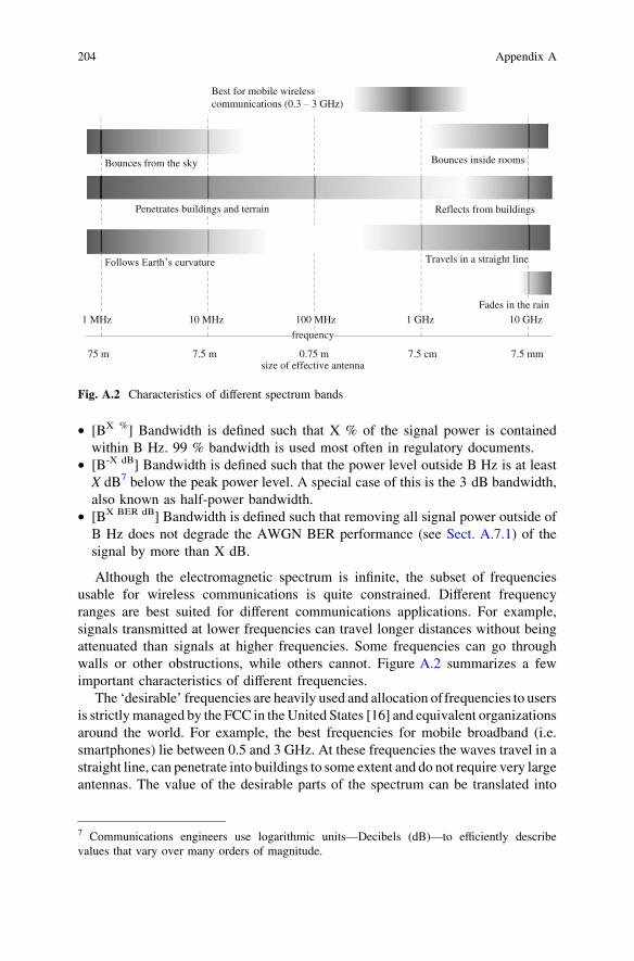
• [BX %] Bandwidth is defined such that X % of the signal power is containedwithin B Hz. 99 % bandwidth is used most often in regulatory documents.
• [B-X dB] Bandwidth is defined such that the power level outside B Hz is at leastX dB7 below the peak power level. A special case of this is the 3 dB bandwidth,also known as half-power bandwidth.
• [BX BER dB] Bandwidth is defined such that removing all signal power outside ofB Hz does not degrade the AWGN BER performance (see Sect. A.7.1) of thesignal by more than X dB.
Although the electromagnetic spectrum is infinite, the subset of frequenciesusable for wireless communications is quite constrained. Different frequencyranges are best suited for different communications applications. For example,signals transmitted at lower frequencies can travel longer distances without beingattenuated than signals at higher frequencies. Some frequencies can go throughwalls or other obstructions, while others cannot. Figure A.2 summarizes a fewimportant characteristics of different frequencies.
The ‘desirable’ frequencies are heavily used and allocation of frequencies to usersis strictly managed by the FCC in the United States [16] and equivalent organizationsaround the world. For example, the best frequencies for mobile broadband (i.e.smartphones) lie between 0.5 and 3 GHz. At these frequencies the waves travel in astraight line, can penetrate into buildings to some extent and do not require very largeantennas. The value of the desirable parts of the spectrum can be translated into
1 MHz 10 MHz 100 MHz 1 GHz 10 GHz
75 m 7.5 m 0.75 m 7.5 cm 7.5 mmsize of effective antenna
Penetrates buildings and terrain
Bounces from the sky
Best for mobile wirelesscommunications (0.3 3 GHz)
frequency
Bounces inside rooms
Reflects from buildings
Travels in a straight line
Fades in the rain
Fig. A.2 Characteristics of different spectrum bands
204 Appendix A
7 Communications engineers use logarithmic units—Decibels (dB)—to efficiently describevalues that vary over many orders of magnitude.

dollars by looking at the results of recent FCC auctions.8 The relationship betweenthe amount of spectrum allocated to a user and how much data throughput that usercan achieve is discussed in the next section. The goal of much of the SDR technologydiscussed in this book is to transmit as much data as possible using the least amountof spectrum (bandwidth) while obeying all the other constraints.
A.3 Channel Capacity
The theoretical foundation for communications theory was laid down by ClaudeShannon in 1948. Starting with the definition of information, Shannon derived anupper bound on the amount of information that can be reliably9 transmitted over acommunications channel. The general formulation of the result is beyond thescope of this book and is elegantly addressed in chapter 7 of [1]. Only a subset ofthe theory applicable to a simple AWGN channel (see A.9.1) is considered in thissection. The capacity of an AWGN channel is given by
C ¼ B log2 1þ SNRð Þ ¼ B log2 1þ P
N
� �¼ B log2 1þ P
BN0
� �
where
B is the bandwidth of the signalP is the average power of the received signalN0 is the noise power density and N is the total noise in the signal bandwidth
This well-known result applies to the simple AWGN channel with a singletransmit and a single receive antenna and with the channel gain constant over thebandwidth of the channel. Shannon’s result proved that this capacity wastheoretically achievable, but provided little insight into how it can be achieved inpractice. At the time his work was published, communications links wereachieving at best 10 % of the predicted capacity. It took another 40 years forcoding theory to develop techniques that now allow us to operate almost atcapacity (see Sect. A.8).
Let us consider a few examples to develop some intuition about what thisfundamental result really means. We first observe that capacity growslogarithmically with the signal power.
Consider a link with B = 1 Hz, N0=1 W/Hz, P=0.1 W. The capacity of this linkis C ¼ 1 log2 1þ 0:1
1�1
� �¼ 0:14 bps. What happens if we double the transmit
power? Capacity increases almost 2-fold to 0.26 bps. What if the transmit power is
Appendix A 205
8 Over $60 billion has been paid by companies to the US treasury over the past 15 years for therights to operate in a few spectral bands.9 With arbitrarily small error probability of error.

1 W? Capacity is then exactly 1 bps. How much extra power would be required todouble this throughput? The total power required to achieve 2 bps is 3 W(SNR = 3)—3 times more than before. The point is clear—the amount of powerrequired to increase throughput grows exponentially! It takes a lot of power toincrease bandwidth efficiency above 1 bps/Hz (due to the shape of the logfunction) (Fig. A.3).
Let us now consider the effect of available bandwidth, B, on the capacity. Athigh SNR, capacity increases almost linearly with bandwidth. Of course, as thebandwidth increases, SNR decreases since more noise enters the system.10
Consider the same link as in the example above: with B = 1 Hz, N0 = 1 W/Hz,P = 0.1 W. How much bandwidth is required to double the capacity? Looking atFig. A.4, we observe that capacity increases slower than logarithmically asbandwidth asymptotically approaches a constant. Thus, capacity cannot bedoubled by simply increasing bandwidth without increasing power! This region ofthe capacity curve is known as power constrained.
Now consider a link with B = 0.1 Hz, N0 = 1 W/Hz, P = 1 W. SNR is 10.When SNR is relatively high, increasing bandwidth helps increase capacity. Forexample, increasing bandwidth by a factor of 4 to 0.4 Hz approximately doublesthe capacity. A corresponding increase in capacity while keeping the bandwidth at0.1 Hz requires about 15 times more power.
These examples demonstrate an important point about channel capacity. At lowSNR (\3 dB), increasing power is an effective way to increase capacity. However,at high SNR ([10 dB), small increase in capacity requires a very large increase inpower. Likewise, increasing bandwidth is not effective at increasing capacity atlow SNR, but becomes effective at high SNR.
0 1 2 3 40
0.5
1
1.5
2
2.5
SNR [linear]
Cap
acity
[bps
]
0 1 2 30
5
10
15
20
Capacity [bps]
Add
itio
nalp
ower
requ
ired
todo
uble
capa
city
[W]
Fig. A.3 AWGN channel capacity and power requirements
10 Exercise for the reader: analyze the asymptotic behavior of the channel capacity as bandwidthtends to infinity.
206 Appendix A

For many wireless links, both power and bandwidth are constrained by applicablestandards and regulatory bodies. A relatively new technology, known as MIMO, hasbeen developed over the last two decades to overcome the bandwidth limitation.
A.4 Transmitting Messages
Messages can be transmitted by varying any observable parameter. Dozens ofdifferent transmission techniques and message formats have been developed overthe years. The conversion between an abstract message and an observable outcomeis known as modulation. The observable outcomes are known as symbols. Symbolsare transmitted at regular intervals (at a constant rate, known as the symbol rate,R). The bandwidth of a signal is proportional11 to its symbol rate, B / R. Theproportionality constant depends on the modulation. This section will mentionsome of the more frequently used modulations.
A.4.1 On-Off Keying
Perhaps the simplest modulation scheme is on-off-keying (OOK). At any symbolinterval, a signal is either transmitted or not. Presence of the signal can be mappedto a ‘1’ and absence of a signal can be mapped to a ‘0.’ The signal itself can beanything:
• Smoke rising from a fire (‘1’) or blocked by an animal hide (‘0’)• A flash of light reflected from a mirror (‘1’) or no flash (‘0’)
0 0.2 0.4 0.6 0.8 10
0.5
1
1.5
2
Bandwidth [Hz]
Cap
acity
[bps
]
Power = 1 W
Power = 15 W
Fig. A.4 AWGN capacityand bandwidth requirements
Appendix A 207
11 For most modulations. Exceptions include PPM described in Sect. A.4.6.

– Modern optical communications is a logical extension of this ancientapproach. Even today, most commercial optical systems rely on simple on/offpulses from a laser.
• A whistle (‘1’) or silence (‘0’)• Nonzero voltage level on a wire (‘1’) or ground potential (‘0’)
A.4.2 Frequency Shift Keying
Frequency shift keying (FSK) is another very simple modulation scheme that hasbeen in use for hundreds of years. FSK symbols differ from each other by thefrequency of the signal. The oldest example is using different colored lanterns.Different colors of light correspond to different frequencies of the electromagneticwave (e.g. blue light is *650 THz, while red light is *450 THz). Whistling orplaying different musical notes uses different frequencies of sound to transmitdifferent messages. Practical FSK modulation uses 2, 4, 8, or 16 closely spacedfrequencies. The spacing between adjacent frequencies relative to the symbol rateis known as the modulation index. The phase of the signal can remain contiguousbetween successive symbols (continuous phase FSK, CPFSK) or start at anarbitrary or random phase at the beginning of each symbol. Since FSK is relativelyeasy to generate and detect it is still used for low-data rate links such as satellitecommand and control.
A.4.3 Continuous Phase Modulation
The continuous phase FSK modulation described above is one of a general class ofcontinuous phase modulations (CPM). Data bits are encoded by smoothlychanging the phase of the output signal from the previous symbol to the newsymbol. Signal amplitude remains constant. The shape of the phase as it changesfrom one symbol to the next (phase trajectory) depends on the specifics of themodulation. The contiguous phase trajectory means that the symbol cannot bedetermined solely from the final phase of the signal. The symbol depends on thefinal phase and the phase at the beginning of the symbol. The phase at thebeginning of the symbol is determined by the cumulative total phase of allprevious transmitted symbols. Practical systems design the phase trajectory suchthat only a finite number of previous symbols have to be considered.
Perhaps the simplest type of CPM is minimum shift keying (MSK). MSK is also aspecial case of CPFSK, with two frequencies and the modulation index equal to 1/2.
The most frequently used type of CPM is GMSK—modulation adopted forGSM (second generation cellular telephony standard), Bluetooth, and many others.The phase trajectory for GMSK is determined by passing the input data through aGaussian filter which creates a smooth phase trajectory.
208 Appendix A

A.4.4 Amplitude and Phase Shift Keying
The vast majority of modern modulation schemes rely on amplitude and/or phaseshift keying. These modulation schemes do not have obvious manifestations likesmoke signals or colored flags. Instead, they should be thought of as a set ofcomplex numbers. Complex number notation is integral to description and analysisof APSK. Each symbol, x, is defined by a magnitude and a phase:12
x ¼ xj j\x ¼ xj jei\x ¼ xj j cos \xð Þ þ i xj j sin \xð Þ ¼ xR þ ixI
A set of symbols is then defined by a set of amplitudes, A, and a correspondingset of phases, h. The actual value of A is usually irrelevant, and only the ratiobetween Ak is important.
xk ¼ Akeihk
The set of symbols is known as a constellation and is usually shown graphicallyas a set of points on a complex plane. Each symbol in the constellation maps to aset of data bits.13 For example, the simplest PSK constellation, known as binaryPSK or BPSK, consists of two symbols {–A, +A}, corresponding to data bits ‘1’and ‘0’. Equivalently BPSK is defined by: A0 ¼ A1 ¼ A; h0 ¼ 0; h1 ¼ p, and isshown in Fig. A.5a. More complex constellations, shown in Fig. A.5b–d, usemultiple phases (4 for QPSK, 8 for 8PSK) and multiple phases and amplitudes (12phases and 3 amplitudes for 16QAM). Special cases of the general constellationdescribed above are described below:14
• If the phase is same for all symbols and only the amplitude changes, theconstellation is known as amplitude shift keying, ASK. ASK is rarely used inmodern digital communications.
(a) (b) (c) (d)
Fig. A.5 Standard APSK constellations: a BPSK, b QPSK, c 8PSK, d 16QAM
Appendix A 209
12 The real part of x, xR, is frequently called the in-phase part (I) while the imaginary part, xI, iscalled the quadrature part (Q).13 Any mapping is allowed, but Gray coded (i.e. binary representation of symbols that are closeto each other differ by only one bit) maps usually result in the best performance.14 Note that some constellations fall under multiple special cases.
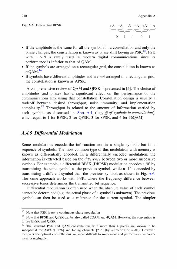
• If the amplitude is the same for all the symbols in a constellation and only thephase changes, the constellation is known as phase shift keying m-PSK.15. PSKwith m [ 8 is rarely used in modern digital communications since itsperformance is inferior to that of QAM.
• If the symbols are arranged on a rectangular grid, the constellation is known asmQAM.16
• If symbols have different amplitudes and are not arranged in a rectangular grid,the constellation is known as APSK.
A comprehensive review of QAM and QPSK is presented in [5]. The choice ofamplitudes and phases has a significant effect on the performance of thecommunications link using that constellation. Constellation design is usually atradeoff between desired throughput, noise immunity, and implementationcomplexity.17 Throughput is related to the amount of information carried byeach symbol, as discussed in Sect. A.1 (log2ð# of symbols in constellationÞ,which equal to 1 for BPSK, 2 for QPSK, 3 for 8PSK, and 4 for 16QAM).
A.4.5 Differential Modulation
Some modulations encode the information not in a single symbol, but in asequence of symbols. The most common type of this modulation with memory isknown as differentially encoded. In a differentially encoded modulation, theinformation is extracted based on the difference between two or more successivesymbols. For example, a differential BPSK (DBPSK) modulation encodes a ‘0’ bytransmitting the same symbol as the previous symbol, while a ‘1’ is encoded bytransmitting a different symbol than the previous symbol, as shown in Fig. A.6.The same approach works with FSK, where the frequency difference betweensuccessive tones determines the transmitted bit sequence.
Differential modulation is often used when the absolute value of each symbolcannot be determined (e.g. the actual phase of a symbol is unknown). The previoussymbol can then be used as a reference for the current symbol. The simpler
+A –A+A +A+A –A
0 1 1 0 1
Fig. A.6 Differential BPSK
210 Appendix A
15 Note that PSK is not a continuous phase modulation16 Note that BPSK and QPSK can be also called 2QAM and 4QAM. However, the convention isto use BPSK and QPSK.17 The standard PSK and QAM constellations with more than 4 points are known to besuboptimal for AWGN [276] and fading channels [275] (by a fraction of a dB). However,receivers for optimal constellations are more difficult to implement and performance improve-ment is negligible.

demodulation comes at the price of reduced performance. Corruption in onesymbol affects two symbol decisions.18 Double differential modulation uses threeconsecutive symbols instead of two [223] to provide even more immunity tofrequency offset at a cost of higher degradation in performance.
A.4.6 Pulse Position Modulation
Pulse position modulation (PPM) relies on transmitting a short pulse at differenttimes within a symbol period. Unlike the previously described modulations, thesignal is transmitted for only a small portion of the symbol period.19 For example, apulse sent in the first half of the symbol period can be mapped to a data bit ‘0’, while apulse in the second half of the symbol period is mapped to ‘1.’ An example is shownin Fig. A.7. Multiple bits can be transmitted by allowing multiple pulse positionswithin a symbol. One of the main difficulties in implementing a PPM is accuratelydetermining the symbol period boundaries. Differential PPM (see Sect. A.4.5) isfrequently used to avoid having to determine the symbol boundaries.
PPM is most often used for optical communications, both over fiber [224] andover the air [225]. RF transmissions using PPM are less common. Short duration ofthe burst makes the PPM waveform wideband (i.e. occupy a large bandwidthrelative to the symbol rate) and has attracted some interest from the ultrawideband(UWB) community [226].
A.4.7 Orthogonal Frequency Division Multiplexing
OFDM is a popular modulation that has been adopted for well over half of allwideband terrestrial standards (including both contenders for fourth generationcellular telephony). This section barely scratches the surface of this sophisticatedmodulation, and the reader is encouraged to see Chap. 12 in [1] for a quick
time
0 0 1 0 1 1
Fig. A.7 Pulse positionmodulation
Appendix A 211
18 Actual performance degradation depends on the details of the modulation and demodulatorimplementation. In the simplest case, an uncoded, hard-decision, coherent D-BPSK demodulatorgenerates twice as many errors as the non-differential demodulator. At high SNR this degradationis small (fraction of a dB), but at low SNR the degradation is up to 3 dB.19 Short burst transmissions can be very desirable for some hardware implementations. Forexample, a laser may be powered from a capacitor that takes a lot longer to charge than discharge.Short bursts result in a wideband signal, making PPM one of the modulations selected for theUWB standard [284].

summary or Chap. 15 in [5]. This section first describes the modulation, and thenexplains why it is so popular.
An OFDM modulation consists of N subcarriers.20 The serial user data stream isconverted to a parallel vector with one or more bits for every used21 subcarrier.The number of bits allocated to each subcarrier corresponds to the modulationselected for that subcarrier (e.g. 1 for BPSK, 3 for 8PSK). The modulation on eachsubcarrier can be different. The bits for each subcarrier are then mapped into amodulated symbol. The symbol modulates a subcarrier of frequency fk (Fig. A.8).So far, this describes a standard FDM waveform (see Sect. A.5.2). The key toOFDM is setting fk ¼ k � fb, where fb is equal to the symbol rate. This frequencyassignment ensures that the subcarriers are packed tightly and still remainorthogonal to each other – no subcarrier interferes with any other subcarrier. Thenumber of subcarriers in practical systems ranges from 64 to 4096. Clearly, a brute
Userdata
Seri
al to
par
alle
l
tjfe 0
tjfe 1
tjfNe
Fig. A.8 Conceptual structure of OFDM modulation (fk = 2pfk for conciseness)
212 Appendix A
20 N is almost always a power of 2 to allow efficient hardware implementation using FFTs.21 Some subcarriers can be designated as ‘unused’ or ‘pilots’, or even allocated to other users inthe case of OFDMA.

force implementation of the block diagram in Fig. A.8 is impractical. All currentlyfielded OFDM systems use an FFT to efficiently multiply the input symbols by aset of complex exponentials. However, an FFT is not essential to an OFDM-likemodulation as discussed in [227, 228].
The primary motivation for OFDM is its performance in a fading environment(see Sect. A.9.3). A wideband single carrier waveform experiences differentchannel gain at different frequencies in the band. This leads to distortion known asintersymbol interference (ISI). ISI caused by a wideband rapidly changing channelis difficult to mitigate. Each subcarrier in a wideband OFDM waveform ‘sees’ asmall portion of the channel bandwidth and the channel gains is essentiallyconstant over the frequencies in the subcarrier band. Thus, no ISI is introduced andno mitigation is necessary. This convenience comes at the price of a small amountof overhead due to the cyclic prefix.
A.4.8 Direct Sequence Spread Spectrum
DSSS is a modulation technique that aims to spread the transmitted signal powerover a bandwidth much larger than the symbol rate. Since the bandwidth is roughlyproportional to the rate of change in the signal, spreading is accomplished bymultiplying the original signal by another signal. The second signal has a muchhigher symbol rate. The symbol rate of the second signal is known as the chip rate.The simplest implementation of a DSSS modulation is shown in Fig. A.9. The datasignal modulated with BPSK is multiplied by a high rate signal, also modulatedwith BPSK. Each ‘bit’ in the high rate signal, known as a chip, is generated using apseudo-random sequence. The final output has transitions at the chip rate andtherefore occupies a bandwidth proportional to the chip rate. The ratio of the chip
symbol period
chip period
data
spre
adin
gse
quen
cetr
ansm
itch
ips
Fig. A.9 Spreading a signal by a high rate chipping sequence (SF = 10, PG = 10 dB)
Appendix A 213

rate to the symbol rate is known as the spreading factor, SF.22 The spreading factoris also expressed as the processing gain, PG = 10 log10(SF).
The receiver multiplies the received signal by a replica of the pseudo-randomcode to get back the original data signal (multiplying each chip by itself effectivelyremoves the spreading since 1 9 1 = 1 and –1 9 – 1 = 1).
Since spectrum is a precious resource, why would it be desirable to increase thebandwidth of a signal? At first glance, it seems quite wasteful. There are threereasons to use DSSS:
1. Security: The total power in the spread and unspread signals is the same. Thenthe power spectral density (power per Hz of bandwidth) is lower for a spreadsignal. For large SF, the power spectral density is very low and can easily belower than the noise floor (i.e. natural noise level in the environment). Thereceiver can still detect the signal by ‘despreading’ it. However, a hostileobserver cannot easily detect that a transmission is even taking place,23 leadingto a low probability of detection (LPD). Even if the transmission is detected, theobserver would have to know the pseudo-random sequence to make sense of thesignal.
2. Multiple Access: Each spread signal appears as noise to other users in the sameband. As long as the pseudo-random sequences for each user are relativelyuncorrelated, multiple users can share the same band at the same time (also seeSect. A.5.5).
3. Multipath Fading Mitigation: As discussed in Sect. A.9.3, multipath fading isusually more detrimental to wideband signals than to narrowband ones.However, efficient receiver architecture exists to mitigate the effects ofmultipath fading on DSSS waveforms. A RAKE receiver (Chap. 13 in [1])recombines delayed replicas of the signal in the time domain to combat fading.
DSSS modulation is used for all third generation cellular telephony standards(3GPP and cdma2000) as well as for some WiFi modes for reasons 2 and 3. It hasbeen replaced by OFDM for the fourth generation of wireless standards.
Most examples of DSSS use either BPSK or QPSK for both data and chippingmodulations. However, it is entirely valid to spread a BPSK data signal with an8PSK chipping sequence.
A.4.9 Frequency Hop Spread Spectrum
FHSS is similar to DSSS in that it aims to spread the transmitted signal power overa bandwidth much larger than the symbol rate. However, instead of using a high-
214 Appendix A
22 The chip edges are aligned with the symbol edges and SF is an integer in a synchronous DSSSwaveform. The chipping rate is independent of the symbol rate (i.e. SF is not necessarily aninteger) in an asynchronous DSSS system. Most modern DSSS systems are synchronous.23 Sophisticated techniques can detect a spread signal below the noise floor.

frequency chipping sequence, the carrier frequency of the signal is varied over thespreading bandwidth. The carrier frequency is changed according to a predefinedformula every hop period. A hop period can consist of many symbol periods (slowhopping) or a fraction of one symbol period (fast hopping). Frequency hoppingwas first used for military electronic countermeasures. Because radiocommunication occurs only for brief periods on a radio channel and thefrequency hop channel numbers are only known to authorized receivers of theinformation, transmitted signals that use frequency hopping are difficult to detector jam.
FHSS is usually easier to implement than DSSS. A popular consumer wirelessstandard, Bluetooth, selected FHSS because it can be easily implemented in a low-power device.
FHSS can be thought of as a special case of TDMA/FDMA multiple accessscheme (see Sect. A.5.4) with a user assigned a different frequency band in eachtime slot.
A.5 Multiple Access
Multiple access techniques specify how different users can access the radiospectrum to communicate with each other. This section introduces some but not allof the commonly used techniques.
A.5.1 Time Division Multiple Access
In the simplest scenario, two users communicate using the same spectrum (samecarrier frequency and bandwidth) by taking turns transmitting and receiving. Thisapproach can be extended to more than two users by giving each user an exclusiveopportunity to transmit at a given time. All other users must not transmit at thesame time, as shown in Fig. A.10. The transmit opportunity is known as a timeslot. TDMA requires that all users have the same concept of time and can timetheir transmissions accurately. Accurate timing can be accomplished using either:
User 1
User 2
User 3
Transmit
Receive
Receive
Receive
Transmit
Receive
Receive
Receive
Transmit
Transmit
Receive
Receive
Receive
Transmit
Receive
time slottime
Fig. A.10 Simple TDMA schedule
Appendix A 215
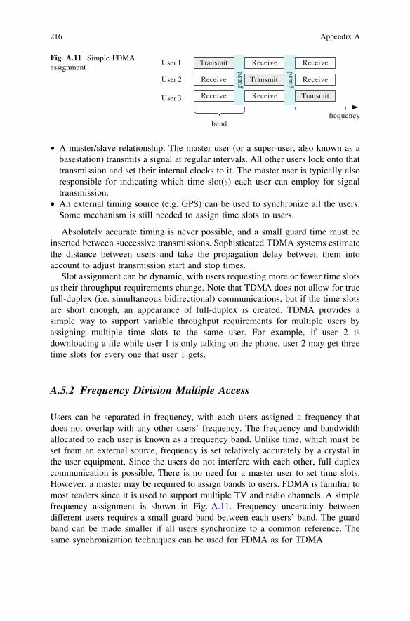
• A master/slave relationship. The master user (or a super-user, also known as abasestation) transmits a signal at regular intervals. All other users lock onto thattransmission and set their internal clocks to it. The master user is typically alsoresponsible for indicating which time slot(s) each user can employ for signaltransmission.
• An external timing source (e.g. GPS) can be used to synchronize all the users.Some mechanism is still needed to assign time slots to users.
Absolutely accurate timing is never possible, and a small guard time must beinserted between successive transmissions. Sophisticated TDMA systems estimatethe distance between users and take the propagation delay between them intoaccount to adjust transmission start and stop times.
Slot assignment can be dynamic, with users requesting more or fewer time slotsas their throughput requirements change. Note that TDMA does not allow for truefull-duplex (i.e. simultaneous bidirectional) communications, but if the time slotsare short enough, an appearance of full-duplex is created. TDMA provides asimple way to support variable throughput requirements for multiple users byassigning multiple time slots to the same user. For example, if user 2 isdownloading a file while user 1 is only talking on the phone, user 2 may get threetime slots for every one that user 1 gets.
A.5.2 Frequency Division Multiple Access
Users can be separated in frequency, with each users assigned a frequency thatdoes not overlap with any other users’ frequency. The frequency and bandwidthallocated to each user is known as a frequency band. Unlike time, which must beset from an external source, frequency is set relatively accurately by a crystal inthe user equipment. Since the users do not interfere with each other, full duplexcommunication is possible. There is no need for a master user to set time slots.However, a master may be required to assign bands to users. FDMA is familiar tomost readers since it is used to support multiple TV and radio channels. A simplefrequency assignment is shown in Fig. A.11. Frequency uncertainty betweendifferent users requires a small guard band between each users’ band. The guardband can be made smaller if all users synchronize to a common reference. Thesame synchronization techniques can be used for FDMA as for TDMA.
frequency
User 1
User 2
User 3
Transmit
Receive
Receive
Receive
Transmit
Receive
Receive
Receive
Transmit
band
guar
d
guar
d
Fig. A.11 Simple FDMAassignment
216 Appendix A

FDMA makes it difficult to respond to changing throughput requirements.While it is possible to allocate multiple bands to a single user, it is not usuallydone24 and all users always get the same throughput.
A.5.3 Random Access
Perhaps the simplest possible multiple access scheme allows all users to transmitwhenever they have data available. Clearly, if two users transmit at the same time inthe same area, the transmissions will collide and neither user succeeds in getting hisdata to the receiver. In that case, the users retransmit after a (typically random) delay.The throughput of such a system, known as pure ALOHA, is quite low if there aremany users.
Carrier sense multiple access (CSMA) improves on pure ALOHA. At any giventime the user checks if another transmission is already taking place (i.e. senses thechannel). If the channel is clear, the user transmits his message. If the channel isbusy, the user either continues sensing until the channel is free (known aspersistent CSMA) or waits a random amount of time to try again. CSMA is verysimple and requires no infrastructure but results in lower overall throughput due tocollisions between users. CSMA is only applicable for packet-based25 data ratherthan streaming data. CSMA has better throughput than ALOHA because thenumber of collisions is reduced. Sensing an ongoing transmission can be difficultand unreliable if a fading channel (see Sect. 3.4), or simply because two trans-mitters cannot ‘see’ each other, as shown in Fig. A.12. In that case, both users 1
Fig. A.12 Hidden user problem with CSMA
Appendix A 217
24 Except in OFDM and OFDMA systems, but those are not strictly speaking FDMA.25 Most modern wireless systems are packet-based.

and 2 ‘sense’ the channel and declare it open. They both transmit to user 3resulting in a collision.
Collision avoidance extends CSMA (CSMA/CA) by having the receivertransmit a busy tone as soon as it starts processing a transmission. Since collisionsoccur at the receiver, the hidden user problem described above is somewhatalleviated. All transmitters close to the receiver now know not to transmit.
A.5.4 Time and Frequency Multiple Access
TDMA and FDMA can be combined to support more users. In the hybrid TDMA/FDMA approach, each user is allocated a time slot and a frequency band it cantransmit in, as shown in Fig. A.13. Taking advantage of both dimensions results ina more flexible schedule and more efficient use of the spectrum. For example, userscan be allocated multiple timeslots and/or bands when they require higherthroughput. The GSM standard uses this approach to support many cellular phonesper basestation.
A.5.5 Code Division Multiple Access
CDMA is only applicable to DSSS modulations described in Sect. A.4.8. Eachuser is assigned a pseudo-random chipping sequence, PNk. The sequences aredesigned such that the peak cross-correlation (H) between any two lengthN sequences is approximately zero:
max PNiHPNj
� �¼ eij � 0 i 6¼ j
N i ¼ j
�
All users then transmit their spread sequences simultaneously in the samefrequency band. Each user can extract the signal intended for him by correlatingthe sum of received signals with his chipping sequence. All other users’ signals
timetime slot
frequency
band User 1
transmit
User 2 transmit
User 3 transmit
User 6 transmit
User 5 transmit
User 4 transmit
User 1 transmit
User 1 transmit
User 3 transmit
User 6 transmit
User 2 transmit
User 2 transmit
Fig. A.13 TDMA/FDMAslot assignment (users 1 and 2get higher throughput)
218 Appendix A

correlate to approximately zero and are treated as noise. An example, shown inFig. A.14, demonstrates the concept for three users.
An obvious question is why an infinite number of signals cannot be transmittedthis way in the same band. Theoretically, this is possible as long as the totalthroughput does not violate the channel capacity theorem (see Sect. A.3) extendedto a multiple access channel (p. 474 in [229]). For relatively simple receivers,26 thenon-zero cross-correlation limits practical number of users that can share thebandwidth [230, 231].
A.5.6 Carrier-in-Carrier (Doubletalk) Multiple Access
A unique multiple access technique was patented about 10 years ago. It allows twousers to share the same band at the same time without using DSSS. To date, thistechnique has only been applied to satellite communications and has very limitedexposure in open literature [232, 233]. It is described here only because of the‘wow’ factor.
The concept is illustrated in Fig. A.15. Two users cannot communicate directlywith each other, and use a satellite to relay their signals. For the purpose of thisexample both users are in the same downlink beam from the satellite (i.e. bothusers receive whatever the satellite transmits). Users require full duplexcommunication, meaning they transmit at the same time. A conventionalapproach would be to use FDMA and allocate each user a frequency band in
Fig. A.14 Code division multiple access
26 I.e. receivers that do not implement multi-user interference cancellation. Interferencecancellation can reduce the effect of non-zero cross-correlation by subtracting the interferingusers’ signals from the received signal.
Appendix A 219
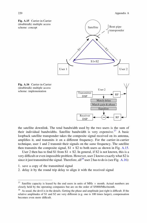
the satellite downlink. The total bandwidth used by the two users is the sum oftheir individual bandwidths. Satellite bandwidth is very expensive.27 A basicloopback satellite transponder takes the composite signal received on its antenna,amplifies it, and transmits it on a different frequency. For the carrier-in-carriertechnique, user 1 and 2 transmit their signals on the same frequency. The satellitethen transmits the composite signal, S1 + S2 to both users as shown in Fig. A.15.
User 2 then has to find S1 from S1 + S2. In general, if S2 is not known, this is avery difficult or even impossible problem. However, user 2 knows exactly what S2 issince it just transmitted the signal. Therefore, all28 user 2 has to do is (see Fig. A.16):
1. save a copy of the transmitted signal2. delay it by the round trip delay to align it with the received signal
S1+S2
Satellite Bent pipe transponder
User 1 User 2
S1 S2
Fig. A.15 Carrier-in-Carrier(doubletalk) multiple accessscheme: concept
TransmitterDSP
ReceiverDSP
Match delay
User 2
RF
RF
Match gain & phase
Equalize
Fig. A.16 Carrier-in-Carrier(doubletalk) multiple accessscheme: implementation
27 Satellite capacity is leased by the end users in units of MHz 9 month. Actual numbers areclosely held by the operating companies but are on the order of $5000/Mhz/month.28 As usual, the devil is in the details. Getting the phase and amplitude just right is difficult. If therelative amplitudes of S1 and S2 are very different (e.g. one is 100 times larger), compensationbecomes even more difficult.
220 Appendix A

3. compensate for gain and phase changes introduced during the trip4. subtract the delayed and adjusted copy from the received signal.
The astute reader will no doubt wonder why the same technique is not usedwithout a satellite in the middle. Why does the approach shown in Fig. A.17 notwork? Why can not User 2 simultaneously transmit and receive? Theoretically, thesame cancellation technique described above should work. In practice, theenormous difference between the power of the transmitted signal and the receivedsignal makes interference cancellation very difficult or impossible. The receiverADC has to sample S1 + S2, where S1 is easily a ten billion (100 dB) timesstronger29 than S1. The main problem is that the output of the power amplifier isnot exactly equal to the signal generated in the transmitter DSP. The thermal andquantization noise present at the input to the amplifier gets scaled together with thesignal. The amplified noise is much higher than the receiver noise floor and cannotbe cancelled out. It may be possible to create a very low noise power amplifier(perhaps a cryogenic one), but such a system is not practical today. Another optionis to put in a high isolation circulator that prevents transmitted signals fromfeeding back to the receiver. Conventional circulators provide about 20 dB ofisolation, which is not nearly enough. However, exotic photonic circulators havebeen reported that may offer sufficient isolation [167].
A.6 MIMO
A relatively new technology, known as multiple-input multiple-output (MIMO),uses multiple antennas at the transmitter and/or receiver to achieve higherthroughput in the same amount of bandwidth. MIMO is a very large and complextopic and is the subject of many books. In this section, we briefly mention some ofthe benefits of MIMO and a qualitative argument for why it works. There are threefundamental methods to take advantage of multiple antennas:
1. Scale and time-align signals for each antenna to form a beam that enhances thedesired signal and suppresses undesired signals. This technique is known asbeamforming (see Sect. 10.5) and has been used for decades.
2. Combat effects of fading by relying on diversity. If each antenna sees an‘independent’ version of the transmitted signal, it is unlikely that all theantennas will experience a ‘fade’ at the same time. Diversity gain is perhaps the
User 1 User 2S1S2
Fig. A.17 Carrier-in-carriermultiple access scheme with-out a satellite
29 For example, a signal transmitted at 2 GHz frequency over 1 km range experiences free spaceloss of *100 dB.
Appendix A 221

most important application of MIMO for terrestrial wireless communications.3. Increase capacity by sending different data on each antenna. This technique,
known as spatial multiplexing, is the most recent application of MIMO.
The first two methods are very effective in the low-SNR regime, while the thirdmethod is most effective in the high-SNR regime. For all of these methods, aMIMO system must have two or more antennas at the receiver, transmitter, orboth. The reader is likely familiar with the first two methods, and only spatialmultiplexing will be discussed below.
The most fundamental results in MIMO were derived by Foscini [234] andTelatar [235]. They showed that the capacity of a channel using Mt transmit andMr receive antennas increases linearly with max (Mt, Mr). This is a dramaticimprovement over the logarithmic growth described in the previous section.MIMO systems achieve capacity that is at first glance higher than Shannoncapacity by creating multiple parallel channels instead of just one. MIMO worksbest in an environment with many multipath. Each path provides another ‘view’ ofthe transmitted signals. Ideally, each antenna should receive a signal uncorrelatedto any other antenna. In a rich multipath environment this can be achieved bysimply separating antennas by at least � of the wavelength of the signal.30 Thereceiver then has many uncorrelated copies of the different transmitted signals andcan apply signal processing to extract each signal.
A simple, but illustrative example is shown in Fig. A.18, where three highlydirectional antennas are used to transmit three separate data streams.31 The beamfrom each antenna does not interfere with other beams. As far as the user isconcerned, each antenna has access to the entire spectrum allocated to him, B. Thetotal bandwidth is therefore 3 9 B. However, the total power available to the userdoes not change and must now be shared between the three antennas. Forsimplicity, assume that the signal from each antenna experiences the same
User 1
S1
S2
S3
User 2
S1
S2
S3
Fig. A.18 Simple MIMO system using highly directional antennas
222 Appendix A
30 MIMO is rarely used at low frequencies because the wavelength is large. Smaller wavelengthallows for smaller antennas and less separation between them. For example, at 3 GHz, thewavelength is 10 cm. Antennas should be separated by at least 2.5 cm. A typical handheld devicecan host not more than two antennas.31 This technique (but without the restriction of directional antennas) is known as VBLAST [277].The antennas are normally not directional. A ‘directional’ link is created by appropriatelycombining signals from all antennas. A matrix defined by the multipath coefficients is inverted andused to multiply the vector of received samples.
m

attenuation and the SNR at all receive antennas is the same.32 The total power isthen shared equally between the antennas, Pk = P/3. The link capacity is then:
C ¼X3
1
B log2 1þ P=3N
� �¼ 3B log2 1þ P=3
N
� �
Relative capacity for B = 1 Hz, for the 3 9 3 antenna MIMO vs. a singleantenna (SISO) is shown in Fig. A.19. As can be seen from that figure, the MIMOsystem achieves almost 39 higher capacity than a SISO system at high SNR. Thelast point is very important—spatial multiplexing becomes effectively only atrelatively high SNR, when the SISO system is in a bandwidth-limited regime (seeSect. A.3). Since MIMO is extremely popular, spatial multiplexing has beensuggested for systems that operate in low SNR and do not experience fading(e.g. satellite links), where the capacity improvement cannot be realized.33 MIMOis applicable for satellite-to-mobile links that experience some fading [236].
SDRs are ideally suited for taking advantage of multiple antennas over a widerange of channel conditions by choosing the appropriate algorithm for different SNRregimes. For example, a SDR can enable full VBLAST processing when average linkSNR is in the 10 dB range. Once SNR falls below 10 dB, additional antennas can bedisabled to save power, or switch to beamforming to achieve power gain.
5 100
10
20
30
SNR [dB]
Cap
acity
[bp
s]
0 15 20 25 300
1
2
3
Cap
acity
impr
ovem
ent r
atio
(3x
MIM
O v
s SI
SO)
Single antenna
Three antennae
Fig. A.19 Capacity for a 3 9 3 MIMO system with uniform SNR
Appendix A 223
32 This is almost never the case and power is allocated to different antennas using the waterfillingalgorithm. The waterfilling algorithm can be shown to be optimal for uncoded systems, but issuboptimal for coded systems [289].33 For example, it does not make sense to use capacity improving MIMO when using a powerfulcode and a robust modulation such as one shown in Figure A.22.

A.7 Performance Metrics
The existence of dozens of different modulations and wireless standards indicatesthat there is no single ‘best’ waveform. Each modulation has advantages anddisadvantages along a set of different metrics. The metrics are given different weightdepending on the system requirements and constraints. A few relevant metrics are:
• Bit error rate performance in the presence of noise: What percentage of bitsis received correctly?
• Bandwidth efficiency: What throughput can be achieved in a given bandwidth.The theoretical limit is given by the channel capacity, but most waveforms arequite far from that limit.
• Implementation complexity: Can the radio implementing the waveform bebuilt within the technology constraints.
• Robustness to interferers: How well will the waveform perform in thepresence of intentional or unintentional interferers.
A.7.1 Bit Error Rate
BER is perhaps the most fundamental, and definitely the most frequently used, metricapplied to wireless waveforms. BER curves show the average fraction of bitsreceived incorrectly versus the energy expended to transmit one bit of data relative tothe noise floor, Eb/N0. Eb/N0 is closely related to the signal to noise ratio.34 BERcurves are also known as waterfall curves because of their characteristic shape, seeFig. A.20. Since each curve captures only the dependence on SNR, all other relevantparameters (e.g. channel type, interference environment) must be annotatedseparately. The BER curve can be used by the system designers to determine therequired transmit power, or the distance over which the link can operate bycomputing these parameters from Eb/N0. Analytical equations have been derived tocompute the BER for almost every uncoded waveform and for a small subset ofcoded waveforms. Most of these equations are only applicable in a pure AWGNchannel, and some are available for fading channels.35
Analytical results are invaluable for providing intuition about what variablesaffect the BER. However, these results are derived for simplified and idealizedoperating environments which are rarely seen in practice. BER curves for aspecific scenario that takes into account all the distortions and degradations are
224 Appendix A
34 The author has sat through many meetings where the exact meaning of the abscissa wasdebated over and over. Some researchers choose to use the symbol rather than bit power, Es/N0,which are not the same if each symbol conveys multiple bits. Others feel that the forward errorcorrection coding should not be considered in the definition of Eb/N0, and use the term ‘channelbit’, Ec/N0. Still others are only comfortable with ‘true’ SNR, or C/N0. Each community has itsown preferences (e.g. GNSS prefers C/N0).35 MATLAB provides a nice compendium of these analytical results via the ‘bertool’ command.

usually obtained by simulating the system. These simulations can be extremelycomputationally intensive and require a long time to complete. One of theapplications of SDR is the simulation of BER curves. Hardware-based SDRs canspeed up these simulations. Of course, the SDR has to implement all the relevantimpairments and degradations. The difference between the simulated curves andthe analytical ones is known as performance loss.
BER curves are used almost universally to compare performance of differentwaveforms. However, it is often the wrong metric. Uniform distribution of errors isan implicit assumption in a BER curve. Consider two ways to get BER = 10 % in aset of 100 bits:
1. 9 correct bits, followed by 1 incorrect bit. The sequence repeats 10 times.2. 90 correct bits followed by 10 incorrect bits.
The first scenario is likely to occur in an AWGN channel with an uncodedwaveform. The second scenario can occur in a fading channel, or if coding isapplied. The impact on the user from these scenarios can be quite different:
a. Live video is transmitted with 10 bits per video frame. In the first scenario, eachframe has a minor glitch that may not be noticeable. In the second scenario, an entireframe is lost which is quite noticeable. Thus, scenario 1 is better than scenario 2.
b. Data is transmitted in packets of 10 bits. Parity is checked on every packet andif the check fails, the packet is discarded. In the first scenario, all packetscontain one error and therefore all are discarded. The packet error rate is100 %. In the second scenario, only the last packet is discarded and the packeterror rate is 10%. Thus, scenario 2 is better than scenario 1.
Packet error rate is a metric more suitable for modern wireless systems. It doesnot matter how many bits in a packet are bad—one invalidates the entire packet.
4 6 8 10 12 1410
-6
10-5
10-4
10-3
10-2
10-1
Eb/N0
BE
R
BPSK in AWGN channelBPSK in Rayleigh channel16-QAM in AWGN channel
Fig. A.20 A few BER curves
Appendix A 225
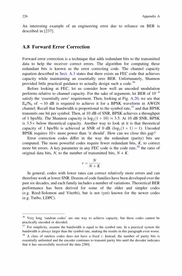
An interesting example of an engineering error due to reliance on BER isdescribed in [237].
A.8 Forward Error Correction
Forward error correction is a technique that adds redundant bits to the transmitteddata to help the receiver correct errors. The algorithm for computing theseredundant bits is known as the error correcting code. The channel capacityequation described in Sect. A.3 states that there exists an FEC code that achievescapacity while maintaining an essentially zero BER. Unfortunately, Shannonprovided little practical guidance to actually design such a code.36
Before looking at FEC, let us consider how well an uncoded modulationperforms relative to channel capacity. For the sake of argument, let BER of 10-6
satisfy the ‘essentially zero’ requirement. Then, looking at Fig. A.20, we see thatEb/N0 of *10 dB is required to achieve it for a BPSK waveform in AWGNchannel. Recall that bandwidth is proportional to the symbol rate,37 and that BPSKtransmits one bit per symbol. Then, at 10 dB of SNR, BPSK achieves a throughputof 1 bps/Hz. The Shannon capacity is log2 1þ 10ð Þ � 3:5. At 10 dB SNR, BPSKis 3.59 below theoretical capacity. Another way to look at it is that theoreticalcapacity of 1 bps/Hz is achieved at SNR of 0 dB (log2 1þ 1ð Þ ¼ 1). UncodedBPSK requires 109 more power than ‘it should’. How can we close this gap?
Error correction codes differ in the way the redundant (parity) bits arecomputed. The more powerful codes require fewer redundant bits, K, to correctmore bit errors. A key parameter in any FEC code is the code rate,38 the ratio oforiginal data bits, N, to the number of transmitted bits, N + K.
r ¼ N
N þ K
In general, codes with lower rates can correct relatively more errors and cantherefore work at lower SNR. Dozens of code families have been developed over thepast six decades, and each family includes a number of variations. Theoretical BERperformance has been derived for some of the older and simpler codes(e.g. Reed-Solomon and Viterbi), but is not (yet) known for the newer codes(e.g. Turbo, LDPC).
226 Appendix A
36 Very long ‘random codes’ are one way to achieve capacity, but these codes cannot bepractically encoded or decoded.37 For simplicity, assume the bandwidth is equal to the symbol rate. In a practical system thebandwidth is always larger than the symbol rate, making the results in this paragraph even worse.38 A class of rateless codes does not have a fixed r. Instead, the number of parity bits isessentially unlimited and the encoder continues to transmit parity bits until the decoder indicatesthat it has successfully received the data [280].

Codes can be classified into two major classes, as shown in Fig. A.21:
1. Block codes work on fixed length sequences of bits. The parity bits depend onlyon the previous N bits. Code performance generally improves (within a codefamily) as the block size increases. Examples of block codes include: Reed-Solomon, Turbo, LDPC. Most modern powerful codes are block codes.
2. Convolutional codes work on sequences of arbitrary length. A feedback loop mayexist in the equation for computing parity bits and the parity bits then depend on theentire history of transmitted bits. Since most modern systems are packet-based,convolutional codes are typically terminated to keep the history a fixed length. Thebest known convolutional code is actually named for the type of decoder used toprocess it – the Viterbi decoder (frequently, but incorrectly, called the Viterbi code).
FEC decoders can be classified into two major classes:
1. Hard-decision decoders work on data bits estimated from the received symbols.2. Soft-decision decoders work on real values that indicate the reliability of the
data bits estimates from the received symbols. For example: BPSK symbolscorresponding to bits ‘0’ and ‘1’ are nominally +1 and –1. Symbols are receivedcorrupted by noise and are digitized to real values {0.7, -0.99, 1.2, 0.2}. Thehard-decisions are then {‘0’, ‘1’, ‘0’, ‘0’}. Clearly some information is lostgoing from the received symbols to hard decisions. Soft-decision decoders takeadvantage of this ‘lost’ information. For example, it is clear that the confidencethat the last symbol is a ‘0’ is a lot lower than for the previous symbol (0.2 is alot closer to -1 than 1.2 is).
Soft-decision decoders provide better performance (by as much as 3 dB,depending on the code), but require more computational resources (at least 49).
A major advance in FEC code design came in the 1980s with the developmentof iterative decoding for Turbo Codes. Prior to iterative decoding, a decodingalgorithm was applied to the received data once. Whatever errors remained afterthe decoding algorithm could not be corrected. The elegant idea of iterativedecoding is to apply the same algorithm multiple times. For specially designedcodes, each application of the decoding algorithm changes the reliability estimates
Block Convolutional
Hamming
BCH
Reed-Solomon LDPC
Turbo
Concatenated
Product
Trellis-codedmodulation
Algebraic (hard-decision) decoding Iterative decoding Viterbi decoding
Fig. A.21 Classification of FEC codes
Appendix A 227

for the data bits.39 The information from data bits with higher confidence is used toincrease the confidence in other data bits. After a number of iterations, allconfidences are expected to converge to large values and decoding is complete.Applying the algorithm many times increases the computational complexity. AnFEC decoder for a modern code such as Turbo and LDPC often dominates thecomputational complexity of the entire modem.
Figure A.22 shows BER performance of a powerful modern code (DVB-S2LDPC, r = �, N = 32kb). The difference between the coded curve and the uncodedcurve is dramatic. The difference between Eb/N0 required to achieve a certain BERfor coded and uncoded waveforms is known as the coding gain. For example, thecoding gain at BER = 10-6 for this code is *9 dB. This gain does come at the priceof reduced bandwidth efficiency—using a rate � code reduces the throughput in agiven bandwidth by a factor of 2. Keeping the same assumptions as in the exampleabove, the throughput achieved by the coded waveform is 0.5 bps/Hz. Theoreticalcapacity of 0.5 bps/Hz is achieved at SNR of -0.3 dB (log2 1� 0:3ð Þ � 0:5). Thecoded waveform requires about 2 dB more power than theoretical minimum, whichis a lot better than 10 dB more for the uncoded waveform.
The coded BER curve is an almost vertical line, very different from therelatively smooth uncoded curve. Powerful modern codes turn the waterfall curvesinto cliffs. This is an important observation that is sometimes overlooked byengineers used to the uncoded systems. In particular, it means that the system doesnot degrade gracefully as SNR decreases. Old, uncoded waveforms, could berelied on to operate with somewhat degraded performance if the SNR droppedbelow the target. Modern waveforms fail completely.
2 4 6 8 10 1210
-8
10-6
10-4
10-2
Eb/N0
BE
R
BPSK in AWGN channel
BPSK coded in AWGN channel
Fig. A.22 Performance ofcoded (DVB-S2 r = � 64 kbblock size) BPSK vs.uncoded
39 Most iterative decoders are also soft-decision decoders. However, this is not necessary andhard-decision iterative decoders exist.
228 Appendix A

A.9 Distortions and Impairments
‘‘Noise is a communications engineer’s best friend. Without it we would not have a job’’f. harris
A radio sends its signal into a hostile environment, bent upon degrading anddestroying the signal before it reaches the intended receiver. The complexity ofthis environment, known as the channel, provides employment to mostcommunications engineers. In addition to impairments introduced by theenvironment, the receiver and transmitter both distort the signal from thetheoretical ideal. In this section, we review some of the most frequentlyencountered channel impairments. The first few subsections cover environmentaleffects, while the last few cover distortions introduced by the hardware.
A.9.1 Thermal Noise
The most fundamental impairment is thermal noise. Thermal noise is usuallyassumed to be a pure random process with Gaussian distributed amplitude and flat(white) spectrum. It is therefore called additive white Gaussian noise (AWGN).AWGN comes from many sources, from the vibration of atoms in the receiverelectronics, to black body radiation from the warm ground, to the backgroundradiation left over from the creation of the universe. Thermal noise exists at allfrequencies (at least from DC to 1012 Hz [2], p. 31) at a constant spectral powerdensity of N0 dBm/Hz.40
The total noise power (variance of the random process) is given byP ¼ k � T � B, where T is the temperature41 in Kelvin, B is the bandwidth inHz, and k is Boltzmann’s constant. At room temperature, N0 = -174 dBm/Hz, anumber ingrained in the mind of every communications engineer.
Systems with only AWGN are analytically tractable and a vast majority ofpublished results assume AWGN. Unfortunately, such systems are few and farbetween. Space communications with highly directional antennas and point-to-point microwave links are some of the examples.42 The channel for terrestrialcommunications such as cellular telephony is considerably more complicated.
Appendix A 229
40 Note that the total power in thermal noise appears to be infinite (constant power density 9
infinite bandwidth). In fact, noise power does decrease at very high frequencies, but is white forall practical purposes for wireless systems. High total power is one reason why it is difficult tobuild a good noise source for laboratory testing. Putting wideband noise into a widebandamplifier can overdrive that amplifier and introduce nonlinear effects. This unexpected effect isoften overlooked even by experienced engineers.41 Cryogenics is used to lower the temperature of the front end (low noise amplifier) of ultra-sensitive radios [262].42 Even these examples are AWGN only to a first degree – second-order effects such as rain andother atmospheric distortions must be considered.

A.9.2 Path Loss
As the electromagnetic wave emitted from the transmitter antenna spreads out, thepower at any given point decreases. This effect is obvious to anyone who has usedthe flashlight—objects closer to the light are brighter. In free space (i.e. line ofsight in a vacuum), power decreases with the square of the distance. The ratio ofreceived power, PR, to transmitted power, PT is given by
PR
PT/ 1
d2f 2
The proportionality constant depends on the specifics of the transmitter andreceiver antennas. The path loss is greater at higher frequencies. The quadraticpath loss is useful for analytical derivations and can be assumed as a first orderestimate for line of sight terrestrial communications. However, it is a grossoversimplification. Signals at some frequencies (e.g. \2 GHz) propagate throughair almost as well as through vacuum, while at other frequencies (e.g. 60 GHz) theatmosphere absorbs most of the signal power due to water and oxygen moleculeresonance. More importantly, most terrestrial communications links arecharacterized by obstructions (e.g. walls) and reflections. Measurements in anurban environment ([2], p. 953) show that path loss is not really quadratic indistance, but the exponent varies from 1.5 to 4, with a mean of about 2.7.
A.9.3 Multipath
As the electromagnetic wave emitted from the transmitter antenna makes its wayto the receiver, the wave reflects off different objects in the path. Each reflectionmay eventually arrive at the receiver with a different power and at a different time.This propagation environment is appropriately called multipath as shown inFig. A.23.
The effects43 of multipath propagation depend on the symbol rate and carrierfrequency of the transmitted signal. An excellent in-depth treatment of themultipath channel is provided in [238] and [239]. Low frequency signals do notreflect well off most objects and few multipath are generated. A multipath channelwith M paths is described by:
y tð Þ ¼XM
m¼1
hmx t � dmð Þ
where dm is the delay of the mth path and hm is the gain of that path.
230 Appendix A
43 One effect familiar to those old enough to have used analog TV sets is ‘ghosting.’ A faint copyof an older image was visible over the normal picture.

The gain is usually expressed relative to the strongest path. The gain is typicallycomplex-valued (i.e. non zero phase), but will be assumed real for the examplesbelow. The multipath coefficients are usually not known a priori and change overtime if the transmitter, the receiver, or anything in the environment is mobile.Multipath propagation has two effects on the received signal:
1. Inter-symbol interference2. Fading
A.9.3.1 Inter-Symbol Interference
As delayed and attenuated copies of the transmitted signal add up at the receiverantenna, the resultant signal is a distorted version of the transmitted one.An example, assuming a BPSK signal at a symbol rate of 106, is shown inFig. A.24. The distortion gets worse at higher symbol rates, where the delaybetween the paths is on the order of (or large than) a symbol duration. The ‘typical’delay between paths depends on the environment and can vary from 100ns to 10lsor even larger. Inter-symbol interference is not a major concern for data ratesbelow 10 ksymbols/s, but must be considered for higher data rates. Leftunmitigated, ISI dominates overall system performance and can preclude
TX
RX
Time
1
3
2
pow
er
1 2 3 Path#
Delay[ ns]
Power[dB]
Phase[deg]
1 0 0 0
2 10 -2 0
3 30 -4 0
Fig. A.23 Multipath propagation
Appendix A 231

communications at data rates above 100 kbps even at very high SNR(Fig. A.2544,45 compare to Fig. A.20).
A number of ISI mitigation approaches have been developed over the years:Adaptive equalization. The multipath channel is a linear system and an
approximate inverse linear system can be designed to cancel the effect of thechannel. The problem can be stated as: find a set of filter coefficients zk such that:
z nð Þ ¼XL
l¼1
zly n� lTð Þ � xðnÞ
Pat
h1
Pat
h2
Pat
h3
Fig. A.24 Effect of inter-symbol interference
0 5 10 15 20 2510
-4
10-3
10-2
10-1
100
Eb/N0 [dB]
BE
R
Flat fading
Low ISI
High ISI
Fig. A.25 Effect of ISI on biterror rate
44 This figure assumes a simple model for multipath – path power decreases linearly with thepath delay. Low ISI assumes 3 total paths, while high ISI assumes 201 total paths. Note the ‘errorfloor’ behavior due to ISI.45 BER curves in a fading channel no longer have the ‘waterfall’ shape, but are closer to straightlines.
232 Appendix A

where T is the sample rate of the digitized signal. T is usually equal to half of thesymbol period, T = �Tb. Adaptive signal processing techniques such as steepestdescent can be applied to minimize x nð Þ � zðnÞj j. Equalization works well as longas the maximum delay is not more than a few symbol periods and the multipathcoefficients change slowly relative to the symbol rate. Unfortunately, neitherrequirement is met for modern high-rate systems that are expected to operate whilethe user is in a moving vehicle.
Direct sequence spread spectrum (see Sect. A.4.8) is another approach tomitigate the effects of multipath. The idea is to increase the apparent symbol rateby converting each data symbol into a sequence of shorter chips. The chip durationis designed such that delays between paths are larger than the chip rate, i.e. dm -
dm-1[Tc. Then each path is treated as a unique signal, demodulated, phase andtiming tracked. The individual signals are then coherently combined byappropriately scaling and delaying the symbols. A receiver that implementssuch an algorithm is known as RAKE. RAKE receivers do not work well if two ormore paths arrive within a chip duration.
Orthogonal frequency division multiplexing (see Sect. A.4.7) takes an oppositeapproach to multipath mitigation by making the symbols much longer. An OFDMsymbol consists of many low-rate subcarriers packed closely in frequency.Multipath will corrupt the beginning (dM seconds) of the long symbol, but most ofthe symbol is untouched. The key idea behind OFDM is to take samples from theend of the symbol and prepend them to the beginning of the symbol. Theprepended samples are known as a cyclic prefix (CP). Cyclic prefix must be longerthan dM. The FFT algorithm used to demodulate OFDM is circular, and any set ofsequential samples can be used for demodulation. The multipath delay, dM, isestimated and the first samples are discarded as shown in Fig. A.26.
A.9.3.2 Frequency Selective Fading
The electromagnetic waves from each path combine at the receiver eitherconstructively or destructively. Fading is best understood by considering the high-frequency carrier rather than the data symbols. The carrier is a sine wavepropagating in space. A delay is then equivalent to a phase shift. A delay of half aperiod (equivalently half a wavelength) is equivalent to a 180� shift, or a signinversion. The wavelength depends on the carrier frequency as k ¼ c=f , where c isthe speed of light. At a carrier frequency of 2 GHz, a wavelength is 15 cm. Adifference in path delay of 0.5 ns (7 cm) results in a phase shift of 180�. Considerthe effect of two paths with path delay equal to half a wavelength as shown inFig. A.27. The two waves combine destructively as shown in Fig. A.28.46 Noamount of signal processing in the receiver can compensate for the lack of inputsignal at the antenna. However, moving either TX or RX a few inches fixes the
Appendix A 233
46 Note that there is almost no ISI in this scenario since the delay between paths is negligiblerelative to the symbol period.

problem. This type of fading is known as fast fading because it changes rapidlyover time if TX or RX is moving.
Wideband signals can be thought of as a many adjacent tones (that is literally thecase for OFDM). Tones of different frequency end up with different phase shifts afterthe same delay and therefore combine to different powers. This is known asfrequency selective fading, where parts of the signal spectrum are affected differentlythan others. Many mitigation techniques have been developed to combat fast fading.
Adaptive equalization is not particularly effective against fast fading because itcannot adapt quickly enough.
A combination of interleaving and forward error correction is effective inmitigating fast fading, if the fade duration is significantly shorter than the span ofthe interleaver. The symbols lost during a fade are randomly spread across theinterleaver and then fixed by the FEC decoder.
OFDM Symbol
CP
Symbol A.2
Symbol A .3
Symbol A.1
Received A
Symbol B.2
Symbol B.3
Symbol B.1
Received B
Symbol C.2
Symbol C.3
Symbol C.1
Received C
dM
Used for demod
(a)
(b)
Fig. A.26 Using cyclic prefix in OFDM to mitigate inter-symbol interference (index .1, 2, 3refers to path number)
RXTXPhase
1
2
Path#
Delay[ ns]
Power[dB] [deg]
1 0 0 0
2 0.5 -0.1 0
Fig. A.27 Two path channel
234 Appendix A

DSSS waveforms rely on the spreading gain to compensate for ‘missing’ partsof the signal. Intuitively, if the spread signal is 10 MHz wide, and 1 MHz of that isfaded, only 10 % of the energy is lost and the signal can still be processed.
OFDM can use channel state information (if available) and put no data on thesubcarriers that fall within the faded frequencies.
The most effective technique, known as antenna diversity, is to use multipleantennas. Consider a receiver with two antennas separated by at least half awavelength. The probability that both antennas experience a deep fade at the sametime is relatively low. More antennas reduce the probability even further. A simplemulti-antenna receiver just selects the antenna with the highest received power andprocesses that signal. More sophisticated receivers take advantage of all theantennas and optimally combine their signals (e.g. using maximal ratio combining,MRC [238], p. 312). Many texts mention that MRC increases the average SNR ofthe link by a factor equal to the number of receiver antennas. While that is true, theeffect is relatively unimportant compared to the dramatically reduced number ofdeep fades (and potential dropped links).
Frequency selective fading can also be caused by atmospheric scintillation. Thiseffect is only relevant for ground-spacecraft links. Scintillation refers to the rapidfluctuation in signal amplitude and phase [240, 241]. The effects are oftenobserved in satellite links and may occur either in the ionosphere due to changes infree electron density or/and in the atmosphere due to changes in pressure,humidity, temperature, etc. Although the mechanism behind scintillation is verydifferent from multipath, the effect is very similar. An early exampledemonstrating the use of SDR to mitigate scintillation effects is described in [242].
A.9.3.3 Statistical Fading Channel Models
The number, magnitude, phase, and delay of multipath all depend on the geometryof the environment between the transmitter and receiver. It is clearly not practicalto evaluate the performance of a radio for all possible combinations of geometricconfigurations. A statistical model of a channel is used to represent ‘typical’environments. Such a model is used to generate time-varying channel coefficients,hm, that can be used to first simulate the performance of radio algorithms and then
-1
0
1
-1
0
1
-1
-0.5
0
0.5
1
Pat
h1
Pat
h2
Fig. A.28 Destructive interference due to multipath
Appendix A 235

verify performance of the hardware.47 There are two types of models: thosederived from highly simplified assumptions about the environment and those basedon fits to measurement data. The ‘derived’ models are analytically tractable andare used in most academic publications. An extensive review of different models isavailable in [238] .
Perhaps the most widely used model, Rayleigh, assumes a large number ofmultipaths arriving from all directions. The Rayleigh model is assumes that eachcoefficient is a complex number with Gaussian distribution for real and imaginaryparts. This model is applicable for dense urban environments where no direct lineof sight exists between the transmitter and the receiver. The rate at which thecoefficients change depends on the carrier frequency and the velocity of the radios.The coefficients are considered uncorrelated over time spans that exceed thechannel coherence time. If a line-of-sight exists between the Tx and Rx, theRayleigh model becomes a Rician model.48 The Rician model adds a constantcoefficient with zero delay.
A.9.4 Rain Attenuation
In addition to solid obstructions such as walls and trees, electromagnetic wavesalso have to contend with propagating through rain. Rain attenuation is of greatconcern to satellite communications because the signal has to go through the depthof the atmosphere filled with rain drops.49 It is a smaller, but non-negligible,problem for long distance microwave links. The amount of attenuation, A, dependson rain intensity, R, and the signal carrier frequency, f. An empirical relation,A ¼ aRb, can be used to estimate the attenuation with coefficients a(f) andb(f) derived from measurement data (Fig. A.29) [243, 244, 245]. When the carrierwavelength is small, the waves get reflected and refracted by the individualraindrops. The effect is most pronounced for carrier frequencies above 10 GHz(wavelength \3 cm) [246]. Rain fading is a relatively slow process since it doesnot usually start raining hard immediately. ACM and power control are effective atmitigating the effects of rain fading.
236 Appendix A
47 Channel emulators are available from many test equipment vendors (e.g.http://www.elektrobit.com/). These emulators typically take in an RF signal from the transmit-ter and output an RF signal to the receiver. Internally, a channel emulator uses one of thestatistical models (or measured data) to filter the digitized input signal. A mid-range emulatorruns $200,000 with MIMO models well over $500,000.48 Equivalently, a Rayleigh model is a special case of the Rician model with the ratio of the LOSpower to the multipath power equal to zero. Note that both models are named after the equationthat describes the distribution of received signal amplitude.49 The effect is no doubt well-known to readers with satellite TV receivers.
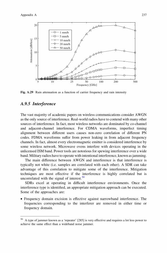
A.9.5 Interference
The vast majority of academic papers on wireless communications consider AWGNas the only source of interference. Real-world radios have to contend with many othersources of interference. In fact, most wireless networks are dominated by co-channeland adjacent-channel interference. For CDMA waveforms, imperfect timingalignment between different users causes non-zero correlation of different PNcodes. FDMA waveforms suffer from power leaking in from adjacent frequencychannels. In fact, almost every electromagnetic emitter is considered interference bysome wireless network. Microwave ovens interfere with devices operating in theunlicensed ISM band. Power tools are notorious for spewing interference over a wideband. Military radios have to operate with intentional interference, known as jamming.
The main difference between AWGN and interference is that interference istypically not white (i.e. samples are correlated with each other). A SDR can takeadvantage of this correlation to mitigate some of the interference. Mitigationtechniques are most effective if the interference is highly correlated but isuncorrelated with the signal of interest.50
SDRs excel at operating in difficult interference environments. Once theinterference type is identified, an appropriate mitigation approach can be executed.Some of the approaches are:
• Frequency domain excision is effective against narrowband interference. Thefrequencies corresponding to the interferer are removed in either time orfrequency domain.
5 10 25 50 100 200 5000
5
10
15
20
Frequency [GHz]
Atte
nuat
ion
[dB
/km
]1 mm/h5 mm/h10 mm/h20 mm/h50 mm/h
Fig. A.29 Rain attenuation as a function of carrier frequency and rain intensity
50 A type of jammer known as a ‘repeater’ [285] is very effective and requires a lot less power toachieve the same effect than a wideband noise jammer.
Appendix A 237

– An adaptive notch filter is tuned to optimally remove the interferer [247] or– The received signal is transformed to the frequency domain using an FFT.
The bins corresponding to the interferer are clipped or zeroed out. Thefrequency domain is then transformed back to the time domain for normalprocessing [248].
• Time domain blanking is effective against wideband bursty interference.• Changing the waveform from DSSS to FHSS is effective against a repeater
jammer.• Changing the waveform from FHSS to DSSS is effective against a frequency
follower jammer.• Multi-user detection (also known as successive interference cancellation) is
effective against a known and uncorrelated interferer.
Unexpected interference types are often encountered once the radio is fielded.SDR allows the waveforms and algorithms to be updated once new mitigationtechniques are developed.
A.9.6 Nonlinearity
Transceiver hardware consists of many analog and RF components that introducenonlinearities into the system.51 Nonlinear distortion is difficult to mitigate and isavoided whenever possible. However, avoiding nonlinear distortion means that allthe components have to operate in their linear regions. Many components,especially amplifiers, are most power efficient outside their linear region.52 Atrade-off exists between power consumption and the amount of distortion. Theeffects of distortion can be seen in both time and frequency domains. In the timedomain, the effect is most obvious when looking at constellation plot, as shown inFig. A.30a. The outer points (points with highest power) are compressed. Manywireless standards limit the level of distortion in the transmitter amplifier byspecifying the maximum error-vector-magnitude (EVM). EVM is a measure ofhow much the distorted constellation differs from an ideal one. In the frequencydomain, the spectrum becomes distorted due to intermodulation. A pulse-shapedspectrum acquires characteristic ‘‘shoulders’’ shown in Fig. A.30b.
Adaptive algorithms such as predistortion at the transmitter [249] and adaptiveLLR computation at the receiver can be used to mitigate the distortion.Intermodulation due to nonlinearity is a major problem for wideband SDRreceivers. Any nonlinearity in the front end LNA can cause a strong
238 Appendix A
51 Fundamentally, no component is completely linear—if nothing else, putting sufficient powerin will cause it to burn up which is a very nonlinear effect.52 Power efficiency also often translates into size and weight. e.g., a less efficient amplifier needsa larger heat sink than a more efficient one.
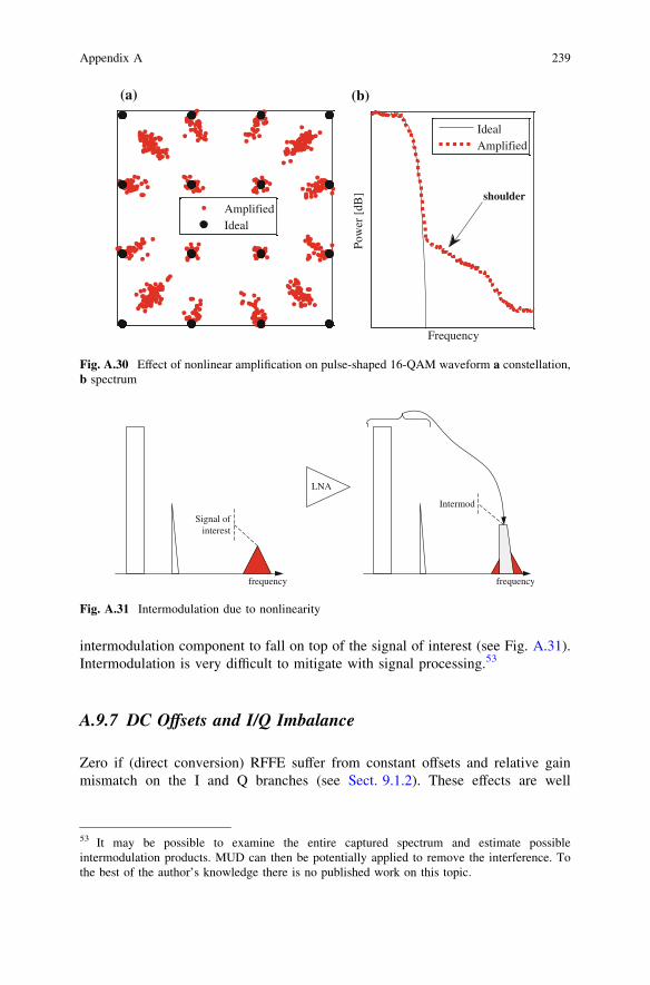
intermodulation component to fall on top of the signal of interest (see Fig. A.31).Intermodulation is very difficult to mitigate with signal processing.53
A.9.7 DC Offsets and I/Q Imbalance
Zero if (direct conversion) RFFE suffer from constant offsets and relative gainmismatch on the I and Q branches (see Sect. 9.1.2). These effects are well
Pow
er [
dB]
Frequency
IdealAmplified
AmplifiedIdeal
shoulder
(b)(a)
Fig. A.30 Effect of nonlinear amplification on pulse-shaped 16-QAM waveform a constellation,b spectrum
frequency
Signal ofinterest
frequency
Intermod
LNA
Fig. A.31 Intermodulation due to nonlinearity
53 It may be possible to examine the entire captured spectrum and estimate possibleintermodulation products. MUD can then be potentially applied to remove the interference. Tothe best of the author’s knowledge there is no published work on this topic.
Appendix A 239

understood and relatively easily mitigated as described [250] and referencestherein. Direct-IF sampling (see Sect. 9.1.3) avoids the problem.
A.9.8 Frequency and Timing Offsets
Frequencies for generating data symbols and the carrier in a radio are typicallyderived from a reference crystal. Each crystal is slightly different,54 making thesymbol rates and carrier frequencies in each radio slightly different. Frequenciesalso vary due to Doppler if the radios are not stationary. One of the first steps inacquiring a signal in the receiver is estimating the relative frequency offsetbetween it and the transmitter. Once the offset is estimated, it must be continuouslyupdated since the offset changes over time. The effect of residual frequency offsetis especially severe for OFDM modulation.
The offsets can be tracked with a feedback loop or can be updated usingfeedforward estimator. The definitive reference to classical phase and timingsynchronization techniques by Mengali [251] should be on every SDR designer’sbookshelf. Synchronization becomes more difficult at low SNR. In fact, thepowerful FEC codes operate at such low SNR that synchronization can become thelimiting factor.
A.9.9 Phase Noise
Frequency offset and drift due to Doppler, crystal aging, and temperature variationchange relatively slowly. However, the crystal also introduces a fast variation inthe phase due to phase noise (also known as jitter). Phase noise is a complexprocess caused by a combination of physical properties of the crystal. It ischaracterized by the power spectral density of the phase variation [252, 253]. Thepower spectral density is specified in units of dBc/Hz—power relative to the toneat the nominal output frequency. Phase noise can be thought of as a random FMmodulation. Instead of a single peak at the nominal frequency, the spectrum of atone spreads out.
Most crystals have more phase noise power close to nominal frequency55 asshown in Fig. A.32. The frequency of a crystal in a radio is scaled up to achievethe carrier frequency (and often the symbol frequency). Typical crystals oscillate
54 Crystal accuracy is specified in parts per million (ppm). For example, a relatively good crystalhas an absolute accuracy of 10 ppm. That means that a symbol rate of 10 MHz is accurate to±100 Hz. A carrier frequency of 2 GHz is accurate to ±20 kHz. Frequency also changes overtime and with temperature. More expensive (and typically larger and higher power) crystals havetighter specifications.55 One notable exception is rubidium atomic clocks which have an essentially constant phasenoise power over frequency.
240 Appendix A

at 1–30 MHz. The phase noise power is increased by the scaling factor.For example, a 10 MHz crystal has phase noise spec of -50 dBc/Hz at 1 kHz
offset. The frequency is multiplied by 100 to get a carrier of 1 GHz. The phasenoise at the carrier is then �50þ 10 log10 100 ¼ �30 dBc/Hz:
Thus, phase noise becomes more of a concern at very high carrier frequencies(e.g. 60 GHz).
The effect of phase noise (just like any other frequency variation) depends onhow frequently the phase estimate is updated in the receiver (usually once persymbol). Phase noise is less of a concern at high symbol rates because the phase isupdated often. Since most of the phase noise power is concentrated at lowerfrequencies, the updates can keep up with the variations in phase and ‘track themout.’ However, at lower data rates, the phase can change by a large amountbetween two updates.
frequency[Hz]
Pow
er [
dBc/
Hz]
10 0 10 1 10 2 10 3 10 4
Fig. A.32 Typical phasenoise profile
Appendix A 241

Appendix BRecommended Test Equipment
Developing a SDR from scratch is a major undertaking. There is a very large gapbetween development of effective baseband DSP algorithms and a working radiosuitable for field use. Most readers will have access to appropriate test equipmentthrough their employers or schools. This section highlights some of the essentialtools of the trade. All modern test equipment is designed to work with a PC forboth control and data transfer. Ethernet interface is preferred to the older GPIB orserial interfaces.
• Digital oscilloscope (2? channel, BW [500 MHz). Must be able to capture atleast 10k samples. Desirable features include:
– Digital inputs (8 or more)
• Spectrum analyzer ([3 GHz). Desirable features include:
– Digital or analog IF output. The SA can be used as a downconverter.
• Vector signal generator ([3 GHz) with I/Q inputs. Desirable features include:
– Integrated baseband signal generator (otherwise an arbitrary waveformgenerator is required).
– Integrated noise generator.
• Two or more SDR development platforms. While it is possible to use a singleboard to both transmit and receive (loopback), two systems are required toverify tracking and acquisition.
– High-end workstation with a programmable RFFE (e.g. USRP) or– FPGA-based platform.
• Channel emulator. A channel emulator should be specific for the intended SDRmarket and capabilities—a MIMO emulator for cellular communications is verydifferent from a satellite channel emulator.
E. Grayver, Implementing Software Defined Radio,DOI: 10.1007/978-1-4419-9332-8, � Springer Science+Business Media New York 2013
243

Optional:
• Arbitrary waveform generator (BW [ 100 MHz).• Noise generator• Logic analyzer. This previously essential tool for debugging digital boards is
becoming less useful with the advent of internal logic analyzers in FPGAs. Aninexpensive logic analyzer can now be quickly rigged up using a cheap FPGAdevelopment board.
244 Appendix B

Appendix CSample XML files for an SCA Radio
The next few paragraphs discuss the contents of XML files used to define an SCAradio. For this example, a very simple SCA application, shown in Fig. C.33, wasdeveloped in OSSIE.56 (Table C.1)
TxDemo RxDemo
complex Short data
Fig. C.33 SCA application
56 Unique identifiers (UIDs) are shortened for compactness
E. Grayver, Implementing Software Defined Radio,DOI: 10.1007/978-1-4419-9332-8, � Springer Science+Business Media New York 2013
245

Table C.1 Software assembly descriptor (SAD) XML file—connecting the components
246 Appendix C

Let us now examine what the SCA OE knows about the TxDemo component.The component is referenced from the SAD file with a link to theTxDemo.spd.xml file, shown in Table C.2. (Tables C.3, C.4, C.5)
Appendix C 247

Table C.2 Software package descriptor (SPD) XML file—setting the executable filename
248 Appendix C

Table C.3 Properties descriptor (PRF) XML file—defining parameters
Appendix C 249

Table C.4 Software component descriptor (SCD) XML file—defining the IO ports
250 Appendix C

Table C.5 Deployment enforcement XML file—defining devices to execute components
Appendix C 251

Bibliography
1. Proakis M (2007) Digital communications. McGraw-Hill, New York2. Sklar B (2001) Digital communications: fundamentals and applications. Prentice-Hall PTR,
Englewood Cliffs3. Wireless Innovation Forum (2011) Driving the future of radio communications and systems
worldwide. http://www.wirelessinnovation.org4. Zimmermann H (1980) OSI reference model–the ISO model of architecture for open
systems interconnection. Commun, IEEE Trans 28:425–4325. Hanzo L, Ng SX, Webb WT, Keller T (2004) Quadrature amplitude modulation: from
basics to adaptive trellis-coded, turbo-equalised and space-time coded OFDM, CDMA andMC-CDMA systems. IEEE Press-John Wiley, New York
6. Caire G, Kumar KR (2007) Information theoretic foundations of adaptive codedmodulation. Proc IEEE 95:2274–2298
7. James JH, Milton S, Bomey Y, Zhong Y (2008) Using FEC, channel Interleaving, ARQ, andDCM to mitigate fades of various timescales. In: 26th international communicationssatellite systems conference (ICSSC)
8. Smolnikar M, Javornik T, Mohorcic M, Berioli M (2008) DVB-S2 adaptive coding andmodulation for HAP communication system. In: Vehicular technology conference, VTCspring 2008, IEEE. pp 2947–2951
9. Sbarounis C, Squires R, Smigla T, Faris F, Agarwal A (2004) Dynamic bandwidth andresource allocation (DBRA) for MILSATCOM. In: Military communications conference,2004. MILCOM 2004, IEEE, vol 2. pp 758–764
10. Kivanc D, Guoqing L, Hui L (2003) Computationally efficient bandwidth allocation andpower control for OFDMA. Wirel Commun, IEEE Trans, vol 2. pp 1150–1158
11. Koffman I, Roman V (2002) Broadband wireless access solutions based on OFDM access inIEEE. Commun Mag, IEEE 40:96–103
12. Rhee W, Cioffi JM (2000) Increase in capacity of multiuser OFDM system using dynamic.In: Vehicular technology conference proceedings, VTC 2000-Spring Tokyo. 2000 IEEE51st, vol 2. pp 1085–1089
13. Mitola J, Maguire GQ (1999) Cognitive radio: making software radios more personal. PersCommun, IEEE 6:13–18
14. Haykin S (2005) Cognitive radio: brain-empowered wireless communications. Sel AreasCommun, IEEE J 23:201–220
15. National Telecommunications and Information Admini (2003) United States frequencyallocations: the radio spectrum. http://www.ntia.doc.gov/osmhome/allochrt.pdf
16. Doumi TL (2006) Spectrum considerations for public safety in the United States. CommunMag, IEEE 44:30–37
E. Grayver, Implementing Software Defined Radio,DOI: 10.1007/978-1-4419-9332-8, � Springer Science+Business Media New York 2013
253

17. Yucek T, Arslan H (2009) A survey of spectrum sensing algorithms for cognitive radioapplications. Commun Surv Tutorials, IEEE 11:116–130
18. Le B et al (2007) A public safety cognitive radio node. In: SDR Forum, Denver19. He A et al (2010) A survey of artificial intelligence for cognitive radios. Veh Technol, IEEE
Trans 59:1578–159220. Mary P, Gorce JM, Villemaud G, Dohler M, Arndt M (2007) Reduced complexity MUD-
MLSE receiver for partially-overlapping WLAN-like interference. In: Vehicular technologyconference, 2007. VTC2007-Spring. IEEE 65th, pp 1876–1880
21. Congzheng Han et al (2011) Green radio: radio techniques to enable energy-efficientwireless networks. Commun Mag, IEEE 49:46–54
22. Gür G, Alagöz F (2011) Green wireless communications via cognitive dimension: anoverview. Network, IEEE 25:50–56
23. Chen Y, Zhang S, Xu S, Li GY (2011) Fundamental trade-offs on green wireless networks.Commun Mag, IEEE 49:30–37
24. Grace D, Chen J, Jiang T, Mitchell PD (2009) Using cognitive radio to deliver ‘Green’communications. In: Cognitive radio oriented wireless networks and communications,CROWNCOM ‘09. 4th international conference on 2009. pp 1–6
25. Viswanath P, Tse DN, Laroia R (2002) Opportunistic beamforming using dumb antennas.Inf Theor, IEEE Trans 48:1277–1294
26. Bogucka H, Conti A (2011) Degrees of freedom for energy savings in practical adaptivewireless systems. Commun Mag, IEEE 49:38–45
27. Popken L (2007) Rescuing the huygens mission from fiasco. Proc IEEE 95:2248–225828. Deutsch LJ (2002) Resolving the cassini/huygens relay radio anomaly. In: IEEE aerospace
conference, Big Sky, MT, pp 3-1295–3-1302. http://trs-new.jpl.nasa.gov/dspace/bitstream/2014/13159/1/01-1802.pdf
29. Vallés EL, Prabhu RS, Dafesh PA (2010) Phase tracking with a cognitive antijam receiversystem (CARS). In: Military communications conference, MILCOM 2010. pp 1701–1706
30. Prabhu RS, Valles EL, Dafesh PA (2009) Cognitive anti-jam radio system. SoftwareDefined Radio Forum, Washington
31. Grayver E et al (2009) Cross-layer mitigation techniques for channel impairments. In:Aerospace conference, 2009 IEEE. pp 1–9
32. Ixia (2011) IxN2X multiservice test solution. www.ixiacom.com/products/ixn2x/index.php33. Grayver E, Chen J, Utter A (2008) Application-layer codec adaptation for dynamic
bandwidth resource allocation. In: Aerospace conference, 2008 IEEE. pp 1–834. Hant J, Swaminathan V, Kim J (2008) Real-time emulation of internet applications over
satellite links using the SAtellite link EMulator (SALEM). In: AIAA, San Deigo35. Murmann B (2008) A/D converter trends: power dissipation, scaling and digitally assisted
architectures. In: Custom integrated circuits conference, 2008. CICC 2008. IEEE. pp 105–11236. Michael LB, Mihaljevic MJ, Haruyama S, Kohno R (2002) A framework for secure
download for software-defined radio. Commun Mag, IEEE 40:88–9637. Dong X (2006) Effect of slow fading and adaptive modulation on TCP/UDP performance of
high-speed packet wireless networks. University of California at Berkeley, Berkeley,Technical Report UCB/EECS-2006-109
38. Kuon I, Rose J (2006) Measuring the gap between FPGAs and ASICs. pp 21–3039. FPGA Developer (2011) List and comparison of FPGA companies. http://www.
fpgadeveloper.com/2011/07/list-and-comparison-of-fpga-companies.html40. Rezgui S, Wang JJ, Sun Y, Cronquist B, McCollum J (2008) New reprogrammable and non-
volatile radiation tolerant FPGA: RTA3P. In: Aerospace conference, 2008 IEEE. pp 1–1141. Microsemi (2011) RT proASIC3 FPGAs. http://www.actel.com/products/milaero/rtpa3/
default.aspx42. Microsemi (2011) Axcelerator antifuse FPGAs. http://www.actel.com/products/axcelerator/
default.aspx
254 Bibliography

43. Palkovic M et al (2010) Future software-defined radio platforms and mapping flows. SigProcess Mag, IEEE 27:22–33
44. Farber R (2011) CUDA application design and development. Morgan Kaufmann45. KHRONOS Group (2011) OpenCL—the open standard for parallel programming of
heterogeneous systems. http://www.khronos.org/opencl/46. Munshi A, Gaster B, Mattson TG, Fung J, Ginsburg D (2011) OpenCL programming guide.
Addison-Wesley Professional, Boston47. Accelereyes (2011) Jacket GPU engine. http://www.accelereyes.com/products48. Kahle JA et al (2005) Introduction to the cell multiprocessor49. Lin Y et al (2007) SODA: a high-performance DSP architecture for software-defined radio.
Micro, IEEE 27:114–12350. Woh M et al (2008) From SODA to scotch: the evolution of a wireless baseband processor.
In: Microarchitecture, 41st IEEE/ACM international symposium on, pp 152–16351. Williston K (2009) Massively parallel processors: who’s still alive?. http://www.eetimes.
com/electronics-blogs/dsp-designline-blog/4034360/Massively-parallel-processors-Who-s-still-alive
52. Schulte Michael et al (2006) A low-power multithreaded processor for software definedradio. J VLSI Sig Process Syst 43(2–3):143–159
53. Mamidi S et al (2005) Instruction set extensions for software defined radio on amultithreaded processor. pp 266–273
54. Coherent Logix (2011) HyperX. http://www.coherentlogix.com/55. Octasic. OCT2224W is a system-on-chip. http://www.octasic.com/en/products/oct2200/
oct2224w.php56. picoChip. PC205 high-performance signal processor. http://www.picochip.com/page/76/57. Tilera. Multicore Processing. http://tilera.com/58. Malone M (2008) On-board processing expandable reconfigurable architecture (OPERA)
program overview. In: The first workshop on fault-tolerant spaceborne computingemploying new technologies. Albuquerque, http://www.zettaflops.org/spc08/Malone-Govt-OPERA-FT-Spaceborne-Computing-Workshop-rev3.pdf
59. Singh K et al (2011) FFTW and complex ambiguity function performance on the maestroprocessor. In: Aerospace conference, 2011 IEEE. pp 1–8
60. Walters JP, Kost R, Singh K, Suh J, Crago SP (2011) Software-based fault tolerance for themaestro many-core processor. In: Aerospace conference, 2011 IEEE. pp 1–12
61. Texas Instruments (2009) OMAPTM 1 processors. http://focus.ti.com/general/docs/wtbu/wtbuproductcontent.tsp?templateId=6123&navigationId=11991&contentId=4670
62. Xilinx (2011) Zynq-7000 extensible processing platform. http://www.xilinx.com/products/silicon-devices/epp/zynq-7000/index.htm
63. Berkeley Design Technology (2006) Enabling technologies for SDR: comparing FPGA andDSP performance. http://www.bdti.com/MyBDTI/pubs/20061115_sdr06_fpgas.pdf
64. Valles EL, Tarasov K, Roberson J, Grayver E, King K (2009) An EMWIN and LRITsoftware receiver using GNU radio. In: Aerospace conference, 2009 IEEE. pp 1–11
65. Feng W, Balaji P, Baron C, Bhuyan LN, Panda DK (2005) Performance characterization ofa 10-gigabit ethernet TOE, high-performance interconnects, symposium on, vol 0, pp 58–63
66. Hughes-Jones R, Clarke P, Dallison S (2005) Performance of 1 and 10 Gigabit ethernetcards with server quality motherboards. Future Gener Comput Syst 21:469–488
67. Schmid T, Sekkat O, Srivastava MB (2007) An experimental study of network performanceimpact of increased latency in software defined radios. pp 59–66
68. Mills D (2007) Network time protocol version 4 protocol and algorithm specification. IETF,RFC 1305
69. Eidson JC, Fischer M, White J (2002) IEEE-1588 standard for a precision clocksynchronization protocol for networked measurement and control systems. IEEE, Standard1588
70. Dobkin DM (2007) The RF in RFID: passive UHF RFID in practice. Elsevier/Newnes, p 34
Bibliography 255

71. Lu G, Lu P (2008) A software defined radio receiver architecture based on clustercomputing. In: Grid and cooperative computing, GCC ‘08, Seventh international conferenceon 2008. pp 612–619
72. Papadimitriou K, Dollas A (2006) Performance of partial reconfiguration in FPGA systems:a survey and a cost model. http://ee.washington.edu/faculty/hauck/publications/KypPartReconfig.pdf
73. Yuan M, Gu Z, He X, Liu X, Jiang L (2010) Hardware/software partitioning and pipelinedscheduling on runtime reconfigurable FPGAs. ACM Trans Des Autom Electron Syst15(2):13:1–13:41
74. McDonald EJ (2008) Runtime FPGA partial reconfiguration. In: IEEE aerospaceconference, Big Sky
75. Suris J et al (2008) Untethered on-the-fly radio assembly with wires-on-demand. In:Aerospace and electronics conference, NAECON 2008, IEEE National. pp 229–233
76. JPEO JTRS (2011) SCA: application program interfaces (APIs). http://sca.jpeojtrs.mil/api.asp
77. Xilinx (2011) Xilinx platform flash XL. http://www.xilinx.com/products/config_mem/pfxl.htm
78. Altera (2011) Altera parallel flash loader megafunction. http://www.altera.com/literature/ug/ug_pfl.pdf
79. Parhi K (1999) VLSI digital signal processing systems: design and implementation. Wiley,New York
80. Hussein J, Klein M, Hart M (2011) Lowering power at 28 nm with Xilinx 7 series FPGAs.Xilinx, white paper WP389
81. Altera (2010) Reducing power consumption and increasing bandwidth on 28 nm FPGAs.White paper WP-01148-1.0
82. Edwards M (1997) Software acceleration using coprocessors: is it worth the effort?. In:Hardware/software codesign, (CODES/CASHE ‘97), Proceedings of the 5th internationalworkshop on 1997. pp 135–139
83. Lange H (2011) Reconfigurable computing platforms and target system architectures forautomatic HW/SW compilation. TUt Darmstadt, Darmstadt, PhD thesis,http://tuprints.ulb.tu-darmstadt.de/2560/
84. Intel (2011) VTuneTM performance analyzer. http://software.intel.com/en-us/articles/intel-vtune-amplifier-xe/
85. Tian X, Benkrid K (2010) High-performance quasi-monte carlo financial simulation: FPGAvs. GPP vs. GPU. ACM Trans Reconfigurable Technol Syst 3(4):26:1–26:22
86. Nallatech PCIe-280–8-lane PCI express 2.0 accelerator. http://www.nallatech.com/Motherboards/pcie-280-8-lane-pci-express-20-accelerator-card-featuring-xilinx-virtex-5-fpga-and-memory.html
87. Nvidia (2011) TESLA C2050 and TESLA C2070 computing processor board. http://www.nvidia.com/docs/IO/43395/BD-04983-001_v04.pdf
88. eVGA (2010) EVGA classified SR-2 motherboard. http://www.evga.com/articles/00537/89. Magma (2011) ExpressBox7 (x8) Gen2. http://magma.com/expressbox7x8G2.asp90. Nallatech (2011) Intel xeon FSB FPGA socket fillers. http://www.nallatech.com/
intel-xeon-fsb-fpga-socket-fillers.html91. XtremeData (2009) XD2000FTM FPGA in-socket accelerator for AMD socket F. http://old.
xtremedatainc.com/index.php?option=com_content&view=article&id=105&Itemid=5992. Reinhart RC et al (2007) Open architecture standard for NASA’s software-defined space
telecommunications radio systems. Proc IEEE 95:1986–199393. JPEO JTRS http://sca.jpeojtrs.mil/home.asp94. Bard J (2007) Software defined radio: the software communications architecture. Wiley,
New York95. Ciaran McHale, CORBA explained simply. http://www.ciaranmchale.com/corba-explained-
simply/
256 Bibliography

96. Balister PJ, Robert M, Reed JH (2006) Impact of the use of CORBA for inter-componentcommunication in SCA based radio. In: SDR forum technical conference, Washington
97. Ulversøy T, Neset JO (2008) On workload in an SCA-based system, with varyingcomponent and data packet sizes. NATO, RTO-MP-IST-083
98. Cormier AR, Dietrich CB, Price J, Reed JH (2010) Dynamic reconfiguration of softwaredefined radios using standard architectures. Phys Commun 3:73–80
99. Stephens DR, Magsombol C, Jimenez C (2007) Design patterns of the JTRS infrastructure.In: Military communications conference, MILCOM 2007, IEEE. pp 1–5
100. Magsombol C, Jimenez C, Stephens DR (2007) Joint tactical radio system—applicationprogramming interfaces. In: Military communications conference, MILCOM 2007, IEEE.pp 1–7
101. ISO/IEC (2002) High-level data link control (HDLC) procedures. http://webstore.iec.ch/preview/info_isoiec13239%7Bed3.0%7Den.pdf
102. National Geospatial-Intelligence Agency (2009) Grids and reference systems.http://earth-info.nga.mil/GandG/coordsys/grids/referencesys.html
103. Reinhart RC et al (2010) Space telecommunications radio system (STRS) architecturestandard. NASA glenn research center, Clevelend, TM 2010-216809
104. Willink E (2002) The waveform description language. Wiley, New York105. Willink ED (2001) The waveform description language: moving from implementation to
specification. In: Military communications conference, MILCOM 2001, communicationsfor network-centric operations: creating the information force, IEEE, vol 1. pp 208–212
106. Scaperoth D et al (2006) Cognitive radio platform development for interoperability. In:Military communications conference, MILCOM 2006, IEEE. pp 1–6
107. Grayver E (2009) Physical layer description standard for software defined radio. SoftwareDefined Radio Forum, Washington
108. Reed Solomon codes as BCH codes http://en.wikipedia.org/wiki/Reed-Solomon_code#Reed-Solomon_codes_as_BCH_codes
109. Comtech, CDM-750 advanced high-speed trunking modem. http://www.comtechefdata.com/products/modems/pCDM-750.asp
110. Pucker L (2005) Does the wireless industry really need all these digital if standards?Commun Mag, IEEE 43:54–57
111. VITA, VITA Radio Transport (VRT) Standard. https://www.vita.com/online-store.html112. Normoyle R, Mesibov P (2008) The VITA radio transport as a framework for software
definable radio architectures. In: Software Defined Radio Forum113. Vigil AJ (2010) Digital IF for MILSATCOM terminals: CONOPS and standardization for
the next decade and beyond. In: Military communications conference, MILCOM 2010.pp 1128–1133
114. thinkRF (2011) WSA4000 RF digitizer. http://www.thinkrf.com/wsa4000_spec.html115. Beljour H et al (2010) Proof of concept effort for demonstrating an all-digital satellite
communications earth terminal. In: Military communications conference, MILCOM 2010.pp 1547–1551
116. MIPI Alliance. DigRF(SM) Specifications http://www.mipi.org/specifications/digrfsm-specifications
117. Seng E (2009) Testing digRF for 3G handsets. Test and Measurement World, May118. Innovative Computer Engineering (2011) SDDS packet format. www.ice-online.com/
BACKUP/SDDSPacket.doc119. OBSAI (2010) RP3 specification. http://www.obsai.org/obsai/documents/public_documents
/download_specifications/rp_specifications120. Lanzani CF (2007) OBSAI RP3-01 6.144 Gbps interface implementation. FPGAworld121. CPRI (2011) Common public radio interface specification. http://www.cpri.info/spec.html122. Varghese AA, Linder LF (2008) Software defined radio—the ‘‘Holy Grail’’ for the industry.
Wirel Des Mag, April 2008
Bibliography 257

123. Intel (2011) Integrated performance primitives (IPP). http://software.intel.com/en-us/articles/intel-ipp/
124. Lu Z (2010) How GNU radio core works—an analysis of GNU radio 3.3.0 sources.http://apachepine.ece.ncsu.edu/resources/How%20GNU%20Radio%20Core%20Works.pdf
125. The GOES-R program office, GOES-R main website. http://www.goes-r.gov/126. National Oceanic and Atmospheric Administration (NOAA) EMWIN-N overview.
http://www.weather.gov/emwin/index.htm127. National Oceanic and Atmospheric Administration (NOAA) LRIT Overview. http://noaasis.
noaa.gov/LRIT128. Mueller K, Muller M (1976) Timing recovery in digital synchronous data receivers.
Commun, IEEE Trans 24:516–531129. Palomo A, Villing R, Farrell R (2008) Software defined radio architectures evaluation. In:
SDR 08 technical conference and product exposition, Washington130. Chen D, Vanhoy G, Beaufait M, Dietrich CB (2010) OSSIE/GNU radio generic component
demonstration. In: SDR ’10 technical conference, Washington131. Prismtech, Spectra CX software communications architecture (SCA) tool. http://www.prism
tech.com/spectra/products/spectra-cx132. CRC, SCARI software suite. http://www.crc.gc.ca/en/html/crc/home/research/satcom/rars/
sdr/products/scari_suite/scari_suite133. Tan K et al (2011) Sora: high-performance software radio using general-purpose multi-core
processors. Commun ACM 54(1):99–107134. Falcao G, Sousa L, Silva V (2011) Massively LDPC decoding on multicore architectures.
Parallel Distrib Syst, IEEE Trans 22:309–322135. Hwang J (2003) Innovative communication design lab based on PC sound card and matlab:
a software-defined-radio OFDM modem example. In: Acoustics, speech, and signalprocessing, Proceedings (ICASSP ‘03), IEEE international conference on 2003, vol 3. ppIII–761-4
136. Beaudoin L et al (2003) Receiving images directly from meteorological satellites in anengineers’ school: technical and pedagogical aspects. In: Geoscience and remote sensingsymposium, 2003, IGARSS ‘03, Proceedings, IEEE international, vol 1. pp 479–481
137. Avtec Systems, Inc (2005) EMWIN OQPSK transmit and receiver prototype specifications.NOAA/CSC, TR 05-004
138. Elektor (2011) Software defined radio. http://www.elektor.com/products/kits-modules/modules/software-defined-radio-%28070039-91%29.91475.lynkx
139. Mathworks (2011) MATLAB and Simulink support for USRPTM devices. http://www.mathworks.com/discovery/sdr/usrp.html
140. National Instruments (2011) What Is NI USRP hardware? http://zone.ni.com/devzone/cda/tut/p/id/12985
141. Hamed Firooz (2011) Implementation of full-bandwidth 802.11b receiver. http://span.ece.utah.edu/pmwiki/pmwiki.php?n=Main.80211bReceiver
142. Sparkfun (2011) SiGe GN3S sampler v2. http://www.sparkfun.com/products/8238143. Borre K, Akos DM (2006) A software-defined GPS and galileo receiver: a single-frequency
approach (applied and numerical harmonic analysis). Birkhäuser, Boston144. NSL (2011) GNSS SDR front end and receiver. http://www.nsl.eu.com/primo.html145. Rincon, DLSR-1U-xx DSPBrik L-band software radio. http://www.rincon.com/DLSR_1U_
xx_Final.pdf146. Midwest Microwave Solutions (2011) VHF/UHF digitizers. http://mms-rf.com/
rf-digitizers.html147. Innovative Computer Engineering, GIGExD. http://www.ice-online.com/rumeL/RI-
GIGEXD.htm148. EPCOS (2007) Front-end solutions for world phones. http://www.epcos.com/web/generator/
Web/Sections/Components/Page,locale=en,r=263282,a=575612.html
258 Bibliography

149. Ghannouchi FM (2010) Power amplifier and transmitter architectures for software definedradio systems. Circ Syst Mag, IEEE 10:56–63
150. Hentschel T (2005) The six-port as a communications receiver. Microwave Theor Tech,IEEE Trans 53:1039–1047
151. Xu X, Wu K, Bosisio RG (2003) Software defined radio receiver based on six-porttechnology. In: Microwave symposium digest, 2003 IEEE MTT-S international, vol 2.pp 1059–1062
152. Agilent Inc (2011) See the future of arbitrary waveform generators. http://www.home.agilent.com/upload/cmc_upload/All/March-1-2011-AWG-webcast.pdf
153. Hunter MT, Kourtellis AG, Ziomek CD, Mikhael WB (2010) Fundamentals of modernspectral analysis. In: AUTOTESTCON, IEEE, pp 1–5
154. Ingels M et al (2010) A 5 mm2, 40 nm LP CMOS transceiver for a software-defined radioplatform. Solid-State Circuits, IEEE J 45:2794–2806
155. Giannini V (2008) Baseband analog circuits for software defined radio. Springer156. Lime Microsystems (2011) Multi-band multi-standard transceiver with digital interface
(LMS6002D). http://www.limemicro.com/download/LMS6002D_Product_Brief.pdf157. Walden RH (2008) Analog-to-digital conversion in the early 21st century. In: Benjamin W
(ed) Wiley encyclopedia of computer science and engineering. Wiley, Hoboken158. Murmann B (2011) ADC performance survey. http://www.stanford.edu/*murmann/
adcsurvey.html159. DARPA Microsystems Technology Office (2009) Remoted analog-to-digital converter with
de-serialization and reconstruction. DARPA, BAA 09-51160. Poberezhskiy YS, Poberezhskiy GY (2004) Sampling and signal reconstruction circuits
performing internal antialiasing filtering and their influence on the design of digitalreceivers and transmitters. Circuits Syst I: Regul Pap, IEEE Trans 51:118–129
161. Schreier R (2005) Understanding delta-sigma data converters. IEEE Press, New York162. Murmann B, Daigle C (2010) DAC survey [private communications]163. Shoop B (2001) Photonic analog-to-digital conversion. Springer, Berlin164. Bussjager R (2006) Photonic analog-to-digital converters. Air Force Research Lab, Rome,
NY, AFRL-SN-RS-TR-2006-109165. Grein ME et al (2011) Demonstration of a 10 GHz CMOS-compatible integrated photonic
analog-to-digital converter. In: CLEO:2011—laser applications to photonic applications, pCThI1
166. Yao J (2009) Microwave photonics. Lightwave Technol, J 27:314–335167. Cox III CH, Ackerman EI (2011) Photonics for simultaneous transmit and receive. In:
International microwave symposium, Baltimore168. Mukhanov OA, Gupta D, Kadin AM, Semenov VK (2004) Superconductor analog-to-digital
converters. Proc IEEE 92:1564–1584169. HYPRES, Inc (2011) Digital-RF receiver. http://www.hypres.com/products/
digital-rf-receiver/170. Gorju G et al (2007) 10 GHz Bandwidth rf spectral analyzer with megahertz resolution
based on spectral-spatial holography in Tm3$?$:YAG: experimental and theoretical study.J Opt Soc Am B 24:457–470
171. Kunkee E et al (2008) Photonically enabled RF spectrum analyzer demonstration172. Colice M, Schlottau F, Wagner KH (2006) Broadband radio-frequency spectrum analysis in
spectral-hole-burning media. Appl Opt 45:6393–6408173. Llamas-Garro I, Brito-Brito Z (2010) Reconfigurable microwave filters. In: Minin I (ed)
Microwave and millimeter wave technologies: from photonic bandgap devices to antennaand applications. Chap. 7, pp 185–205
174. K&L Microwave (2011) Tunable filter products. http://www.klmicrowave.com175. Roy MK, Richter J (2006) Tunable ferroelectric filters for software defined tactical radios.
In: Applications of ferroelectrics, isaf ‘06, 15th IEEE international symposium on the 2006.pp 348–351
Bibliography 259

176. Agile RF (2011) http://www.agilerf.com/products/filters.html177. Wang X, Bao P, Jackson TJ, Lancaster MJ (2011) Tunable microwave filters based on
discrete ferroelectric and semiconductor varactors. Microwaves, Antennas Propag, IET5:776–782
178. Kwang C, Courreges S, Zhiyong Z, Papapolymerou J, Hunt A (2009) X-band and Ka-bandtunable devices using low-loss BST ferroelectric capacitors. In: Applications offerroelectrics, ISAF 2009. 18th IEEE international symposium on the 2009, pp 1–6
179. Hittite Microwave Corporation (2011) Tunable bandpass filters. http://www.hittite.com/products/index.html/category/342
180. Fjerstad RL (1970) Some design considerations and realizations of iris-coupled YIG-tunedfilters in the 12–40 GHz region. Microwave Theory Tech, IEEE Trans 18:205–212
181. OMNIYIG, INC (2011) http://www.omniyig.com/182. Giga-tronics (2011) http://www.gigatronics.com/product/c/tunable-microwave-filters183. Teledyne Microwave, YIG filter information. http://www.teledynemicrowave.com/pdf_
YIG/Teledyne%20Microwave%20YIG%20Filter%20Products%200507.pdf184. Entesari K (2006) Development of high performance 6–18 GHz tunable/switchable RF. The
University of Michigan, Ann Arbor, PhD thesis185. Alipour P et al (2011) Fully reconfigurable compact RF photonic filters using high-Q silicon
microdisk resonators. In: Optical fiber communication conference and exposition (OFC/NFOEC), 2011 and the national fiber optic engineers conference, pp 1–2
186. Norberg EJ, Guzzon RS, Parker JS, Johansson LA, Coldren LA (2011) Programmablephotonic microwave filters monolithically integrated in InP–InGaAsP. Lightwave Technol,J 29:1611–1619
187. Savchenkov AA et al (2009) RF photonic signal processing components: from high ordertunable filters to high stability tunable oscillators. In: Radar conference 2009. IEEE, pp 1–6
188. Constantine Balanis (2005) Antenna theory: analysis and design. Wiley, New york189. Cetiner BA et al (2004) Multifunctional reconfigurable MEMS integrated antennas for
adaptive MIMO systems. Commun Mag, IEEE 42:62–70190. Maddela M, Ramadoss R, Lempkowski R (2007) PCB MEMS-based tunable coplanar patch
antenna. In: industrial electronics, ISIE 2007. IEEE international symposium on 2007,pp 3255–3260
191. Huang L, Russer P (2008) Electrically tunable antenna design procedure for mobileapplications. Microwave Theory Tech, IEEE Trans 56:2789–2797
192. Lee EY et al (2009) The software defined antenna: measurement and simulation of a 2element array. In: Antennas and propagation society international symposium, 2009.APSURSI ‘09. IEEE, pp 1–4
193. Kumar R (2011) Plasma antenna. Lambert Academic Publishing194. Jenn DC (2003) Plasma antennas: survey of techniques and the current state of the art.
Naval Posgraduate School, Monterrey, CA, technical report NPS-CRC-03-001195. Plasma Antennas (2011) PSiAn plasma antennas. http://www.plasmaantennas.com196. AARONIA AG (2011) Logarithmic periodic antenna. http://www.aaronia.com/Datasheets/
Antennas/Broadband_Measurementantenna_HyperLOG3000.pdf197. Zhao J, Chen C-C, Volakis JL (2010) Low profile ultra-wideband antennas for software
defined radio. In: Antennas and propagation society international symposium (APSURSI),2010 IEEE, pp 1–4
198. IBM, Rational DOORS. http://www.ibm.com/software/awdtools/doors/199. OSRMT (2010) Open source requirements management tool. http://sourceforge.net/
projects/osrmt/200. Lamsweerde A (2009) Requirements engineering : from system goals to UML models to
software specifications. Wiley, New York201. Bailey B (2010) ESL models and their application electronic system level design and
verification in practice. Springer, Berlin
260 Bibliography

202. Fingeroff M (2010) High-level synthesis: blue book. Xlibris Corporation Mentor GraphicsCorporation, Philadelphia
203. Knapp D (1996) Behavioral synthesis: digital system design using the synopsys behavioralcompiler. Prentice Hall PTR, Englewood Cliffs
204. Cong J et al (2011) High-level synthesis for FPGAs: from prototyping to deployment.Comput. Aided Des Integr Circ Syst, IEEE Trans 30:473–491
205. Morris K (2011) C to FPGA: who’ll use the next generation of design tools? Electron Eng J,June 2011. http://www.eejournal.com/archives/articles/20110621-nextgen/
206. Xilinx (2011) System generator for DSP. http://www.xilinx.com/tools/sysgen.htm207. Altera (2011) DSP builder/simulink. http://www.altera.com/technology/dsp/dsp-builder/
dsp-simulink.html208. Mathworks (2011) Simulink HDL coder. http://www.mathworks.com/products/slhdlcoder/209. Synopsys (2011) High-level synthesis with synphony model compiler. http://www.
synopsys.com/Systems/BlockDesign/HLS/Pages/Synphony-Model-Compiler.aspx210. Zoss R, Habegger A, Bandi V, Goette J, Jacomet M (2011) Comparing signal processing
hardware-synthesis methods based on the matlab tool-chain. pp 281–286211. Levine DL, Flores-Gaitan S, Gill CD, Schmidt DC (1999) Measuring OS support for real-
time CORBA ORBs. In: Object-oriented real-time dependable systems. Proceedings, 4thinternational workshop on 1999, pp 9–17
212. Wind River (2011) Workbench. http://www.windriver.com/products/workbench/213. TenAsys Corporation (2011) INtime for windows. http://www.tenasys.com/products/
intime.php214. Lynuxworks (2011) LynxOS RTOS. http://www.lynuxworks.com/rtos/rtos.php215. ATLAS (2011) Automatically tuned linear algebra software. http://math-atlas.
sourceforge.net/216. Yang X (2004) A feasibility study of UML in the software defined radio. In: Electronic
design, test and applications. DELTA 2004, 2nd IEEE international workshop on 2004,pp 157–162
217. Dohler M, Heath RW, Lozano A, Papadias CB, Valenzuela RA (2011) Is the PHY layerdead? Commun Mag, IEEE 49:159–165
218. Rappaport TS (2002) Wireless communications: principles and practice. Prentice Hall PTR,Englewood Cliffs
219. Haykin M (2009) Communication systems. Wiley, New York220. Reed JH (2002) Software radio: a modern approach to radio engineering. Prentice Hall,
Englewood Cliffs221. Johnson WA (2004) Telecommunication breakdown: concepts of communication
transmitted via software-defined radio. Pearson Education Inc, New York222. Kenington PB (2005) RF and baseband techniques for software defined radio. Artech
House, London223. Bhatnagar MR, Hjorungnes A (2007) SER expressions for double differential modulation.
In: Information theory for wireless networks, IEEE information theory workshop on 2007,pp 1–5
224. Shiu D-S, Kahn JM (1999) Differential pulse-position modulation for power-efficientoptical. Commun, IEEE Trans 47:1201–1210
225. Park H, Barry JR (2004) Trellis-coded multiple-pulse-position modulation for wirelessinfrared communications. Commun, IEEE Trans 52:643–651
226. Aiello GR, Rogerson GD (2003) Ultra-wideband wireless systems. Microwave Mag, IEEE4:36–47
227. Lin Y-P, Phoong S-M, Vaidyanathan PP (2010) Filter bank transceivers for Ofdm and Dmtsystems. Cambridge University Press, Cambridge
228. Waldhauser DS, Nossek JA (2006) Multicarrier systems and filter banks. Advances in radioscience. http://www.adv-radio-sci.net/4/165/2006/ars-4-165-2006.pdf
Bibliography 261

229. Goldsmith Andrea (2005) Wireless communications. Cambridge University Press,Cambridge
230. Welch L (1974) Lower bounds on the maximum cross correlation of signals. Inf Theory,IEEE Trans 20:397–399
231. Massey JL, Mittelholzer T (1991) Welchs bound and sequence sets for code-divisionmultiple-access systems, pp 63–78
232. Jayasimha S, Paladugula J (2008) Interference cancellation in satcom and ranging. In:National conference on communications
233. Comtech EF Data, DoubleTalk carrier-in-carrier performance characterization. http://www.appsig.com/documentation/dt_cnc_performance.pdf
234. Foschini GJ (1996) Layered space–time architecture for wireless communication in a fadingenvironment when using multielement antennas. Bell Labs Tech J 41–59
235. Telatar E (1995) Capacity of multiantenna Gaussian channels. AT&T, Tech Memo236. Arapoglou P-D, Burzigotti P, Bertinelli M, Bolea-Alamanac A, De Gaudenzi R (2011) To
MIMO or not to MIMO in mobile satellite broadcasting systems. Wirel Commun, IEEETrans 10:2807–2811
237. Huang KD, Malone D, Duffy KR (2011) The 802.11 g 11 Mb/s rate is more robust than6 Mb/s. Wirel Commun, IEEE Trans 10:1015–1020
238. Parsons J (2000) The mobile radio propagation channel. Wiley, New York239. Sklar B (1997) Rayleigh fading channels in mobile digital communication systems.
Commun Mag, IEEE 35:90–100240. Crane RK (1977) Ionospheric scintillation. Proc IEEE 65:180–199241. Moulsley T, Vilar E (1982) Experimental and theoretical statistics of microwave amplitude
scintillations on satellite down-links. Antennas Propag, IEEE Trans 30:1099–1106242. Filip M, Vilar E (1990) Adaptive modulation as a fade countermeasure. An olympus
experiment. Int J Satell Commun 8:31–41243. Olsen R, Rogers D, Hodge D (1978) The aRbrelation in the calculation of rain attenuation.
Antennas Propag, IEEE Trans 26:318–329244. Lin D-P, Chen H-Y (2002) An empirical formula for the prediction of rain attenuation.
Antennas Propag, IEEE Trans 50:545–551245. Willis MJ Rain effects. http://www.mike-willis.com/Tutorial/PF10.htm246. Willis MJ (1991) Fade countermeasures applied to transmissions at 20/30 GHz. Electron
Commun Eng J 3:88–96247. Amin MG, Wang C, Lindsey AR (1999) Optimum interference excision in spread spectrum
communications. Sig Process, IEEE Trans 47:1966–1976248. Ouyang X, Amin MG (2001) Short-time fourier transform receiver for nonstationary. Sig
Process, IEEE Trans 49:851–863249. Tarasov KN, McDonald EJ, Grayver E (2008) Power amplifier digital predistortion—fixed
or adaptive? In: Military communications conference, MILCOM 2008, IEEE, pp 1–7250. Nezami MK (2002) Performance assessment of baseband algorithms for direct conversion
tactical software defined receivers: I/Q imbalance correction, image rejection, DC removal,and channelization. In: MILCOM 2002, Proceedings, vol 1. pp 369–376
251. Mengali U (1997) Synchronization techniques for digital receivers. Plenum Press, New York252. Rutman J, Walls FL (1991) Characterization of frequency stability in precision frequency.
Proc IEEE 79:952–960253. Ferre-Pikal ES et al (1997) Draft revision of IEEE STD 1139–1988 standard definitions of.
In: Frequency control symposium. Proceedings of the 1997 IEEE international, pp 338–357254. Hogg J, Bordeleau F (2010) SCA deployment management: bridging the gap in SCA
development. http://www.zeligsoft.com/files/whitepapers/SCA-Deployment-Management-WP.pdf
255. Fast Infoset http://en.wikipedia.org/wiki/Fast_Infoset256. Bayer M (2005) Analysis of binary XML suitability for NATO tactical messaging. Naval
Postgraduate School, Masters thesis, ADA439540
262 Bibliography
257. XML Query http://www.w3.org/XML/Query/258. Bard J (2007) Software defined radio. Wiley, New York259. Microsoft (2011) Microsoft research software radio (Sora). http://research.microsoft.com/
en-us/projects/sora/260. Texas Instruments (2011) ADS1675: 4MSPS, 24-Bit analog-to-digital converter.
http://focus.ti.com/docs/prod/folders/print/ads1675.html261. Xilinx (2009) Xilinx Virtex-4 configuration guide. www.xilinx.com/support/documentation/
user_guides/ug071.pdf262. Clauss RC (2008) Cryogenic refrigeration systems. In: Low-noise systems in the deep space
network. Jet Propulsion Laboratory, Pasadena, Chap. 4, p 161263. Xilinx (2010) Radiation-hardened, space-grade Virtex-5QV device overview. http://www.
xilinx.com/support/documentation/data_sheets/ds192_V5QV_Device_Overview.pdf264. iBiquity, HD Radio. http://www.hdradio.com/265. World DAB, Digital multimedia broadcasting. http://www.worlddab.org/266. Neo WC et al (2006) Adaptive multi-band multi-mode power amplifier using integrated
varactor-based tunable matching networks. Solid-State Circuits, IEEE J 41:2166–2176267. Yumin Lu, Peroulis D, Mohammadi S, Katehi LP (2003) A MEMS reconfigurable matching
network for a class AB amplifier. Microwave Wirel Compon Lett, IEEE 13:437–439268. Hadzic I, Udani S, Smith J (1999) FPGA viruses. In: 9th international workshop on field-
programmable logic and applications, Glasgow, UK269. Chen SY, Kim N-S, Rabaey JM (2008) Multi-mode sub-Nyquist rate digital-to-analog
conversion for direct waveform synthesis. In: Signal processing systems, 2008. SiPS 2008,IEEE workshop on 2008. pp 112–117
270. Murmann B (2008) A/D converter trends: power dissipation, scaling and digitally assistedarchitectures. In: Custom integrated circuits conference, CICC 2008. IEEE, pp 105–112
271. Courreges S et al (2010) Back-to-back tunable ferroelectric resonator filters on flexibleorganic substrates. Ultrason, Ferroelectr Freq Control, IEEE Trans 57:1267–1275
272. Alexeff I et al (2005) Advances in plasma antenna design. In: Plasma science, ICOPS ‘05.IEEE conference record—abstracts. IEEE international conference on 2005. pp 350–350
273. Dominic Tavassoli (2011) Ten steps to better requirements management. http://public.dhe.ibm.com/common/ssi/ecm/en/raw14059usen/RAW14059USEN.PDF
274. Gaudet VC, Gulak PG (2003) A 13.3-Mb/s 0.35 lm CMOS analog turbo decoder IC with aconfigurable interleaver. Solid-State Circuits, IEEE J 38:2010–2015
275. Huang J, Meyn S, Medard M (2006) Error exponents for channel coding with application tosignal constellation design. Sel Areas Commun, IEEE J 24:1647–1661
276. Sayegh S (1985) A condition for optimality of two-dimensional signal constellations.Commun, IEEE Trans 33:1220–1222
277. Foschini GJ, Golden GD, Valenzuela RA, Wolniansky PW (1999) Simplified processing forhigh spectral efficiency wireless. Sel Areas Commun, IEEE J 17:1841–1852
278. Mitola J (2000) Cognitive radio: an integrated agent architecture for software defined radio.Royal Institute of Technology (KTH), Kista, Sweden, PhD thesis, ISSN 1403-5286
279. Jensen K, Weldon J, Garcia H, Zettl A (2007) Nanotube radio. Nano Lett 7:3508–3511280. Bonello N, Yang Y (2011) Myths and realities of rateless coding. IEEE Commun Mag
9(8):143–151281. Cavallaro JR, Vaya M (2003) Viturbo: a reconfigurable architecture for Viterbi and turbo
decoding. In: Acoustics, speech, and signal processing, Proceedings, (ICASSP ‘03). IEEEinternational conference on 2003, vol 2. pp II–497–500
282. Xilinx (2011) Xilinx partial reconfiguration. http://www.xilinx.com/tools/partial-reconfiguration.htm
283. Altera (2011) Stratix V FPGAs: ultimate flexibility through partial and dynamicreconfiguration. http://www.altera.com/products/devices/stratix-fpgas/stratix-v/overview/partial-reconfiguration/stxv-part-reconfig.html
Bibliography 263

284. Reed JH (2005) An introduction to ultra wideband communication systems. Prentice HallPTR, Englewood Cliffs
285. Wang H, Guo J, Wang Z (2007) Feasibility assessment of repeater jamming technique forDSSS. In: Wireless communications and networking conference, WCNC 2007. IEEE,pp 2322–2327
286. Tabula (2011) Spacetime 3D architecture. http://www.tabula.com/technology/technology.php
287. Rondeau T (2011) VOLK and GNU radio. In: NEWSDR, Boston, http://people.bu.edu/mrahaim/NEWSDR/Presentations/NEWSDR_Rondeau2.pdf
288. Techma (2011) NeXtMidas. http://nextmidas.techma.com/289. Kostina V, Loyka S (2011) Optimum power and rate allocation for coded V-BLAST:
instantaneous optimization. Commun, IEEE Trans 59:2841–2850290. Knuth D (1974) Structured programming with go to statements. ACM J Comput Surv
6(4):268291. Fog A (2011) Software optimization resources. http://www.agner.org/optimize/292. Shrestha R, Mensink E (2006) A wideband flexible power upconverter for software defined
radios. pp 85–89293. Simon A (2002) The COT planning guide: tips, tactics, and strategies for successful IC
outsourcing. Simon Publications, Bethesda
264 Bibliography

Index
AA/D converters, 7Adaptive coding and
modulation, 10, 30Adaptive equalization, 232Additive white
Gaussian noise, 229Adjacent channel interference, 203Analog radio, 1Antenna, 1, 92, 128, 157
adaptive 180diversity, 235
ARQ, 30, 32ASIC, 37, 51, 84, 188
BBandwidth efficiency, 10, 12, 14, 206,
224, 228Beam pattern, 178Beamforming, 178, 221Blanking, 238
CCarrier frequency, 7, 21, 22, 94, 109, 152, 153,
160, 179, 203Channel, 71Channel emulator, 31, 70, 236, 243Channel selection, 7Chip, 214Coding gain, 228Cognitive radio, 9, 21, 25, 65
cognition engine, 23Coherence time, 236
Connectorized, 166Constellation, 209Cost, 2, 20, 27, 37, 47, 54, 95, 109, 123, 136,
137, 140, 148, 159, 166, 190, 194, 245Cyclic prefix, 213, 233
DDatapath, 44, 47, 75, 190DBRA, 17Desirements, 160Direct rf synthesis, 152Direct-if, 155, 165, 239Diversity, 221Doppler, 28, 240DSP, 2, 43DSSS, 53, 57, 64, 213, 214, 235, 238
asynchronous, 214DVB-S2, 14, 118
EEb/N0, 224Effective number of bits, 167Error correcting code, 226Error floor, 232Error-vector-magnitude, 238Event driven, 136Excision, 237
FFast Fading, 13, 233FCC, 10, 21, 22, 204
E. Grayver, Implementing Software Defined Radio,DOI: 10.1007/978-1-4419-9332-8, � Springer Science+Business Media New York 2013
265

F (cont.)Feedback loop, 240Feedforward estimator, 240FHSS, 238Firmware, 61FPGA, 16, 38, 44, 54, 60, 73, 84, 140, 183,
188, 190Frequency shift keying, 208
GGNU Radio, 69, 131
GRC, 188GPP, 55, 73GPU, 47Green radio, 25Guard time, 216
HHandover, 20Hardware acceleration, 53, 65, 84
FPGA, 91Hidden node problem, 23
IIncumbent user, 22Intel IPP, 138Interference, 29Intermodulation, 8, 238IQ mixer, 154Iterative decoding, 227
JJammer, 29, 238
MMaximal ratio combining, 235Modem hardware abstraction layer, 101, 107Modulation, 207Modulation index, 208Multi user detection, 238Multipath, 230Multiuser detection, 24
NNonlinear distortion, 238
OObject Request Broker, 100OFDM, 17, 233, 240On-off-keying, 207Opportunistic beamforming, 27OSSIE, 100, 117, 131, 140, 194, 245
PPacket, 16, 73Parity, 3, 126, 226Partial reconfiguration, 17, 60, 62, 68Performance loss, 225Phase noise, 240Physical layer, 5Power consumption, 5, 10, 24, 27, 38, 48, 52,
55, 81, 154, 158, 165, 172Primary user, 21Profiling, 85, 195
QQ factor, 174Q-factor, 157Quadrature IF mixer, 154
RRateless codes, 226Rayleigh model, 236RF front end, 2, 38, 145RF front ends, 118
SShannon limit, 10, 26, 199, 205Signal acquisition, 3, 186, 57, 61, 138, 65Signal processing workstation (SPW), 187Simulink, 187Skeleton, 100Software controlled, 6Spatial multiplexing, 222Spectrum sensing, 22SPU, 47STRS, 97, 108Stub, 100Symbol, 202Symbol rate, 208Symbols, 207Synchronization, 240SystemVue, 187, 192
266 Index

TTesting, 39Tilera, 49Time slot, 216Tradeoffs, 8
VVITA-49, 93, 94, 118, 122, 123, 145, 146, 149VRT. See VITA-49
WWaterfall curves, 224Waterfilling, 223Waveform, 5Wireless innovation forum, 5
ZZero-if, 239
267 Index