Implicit Runge-Kutta schemes for optimalcontrol problems with evolution equations

Thomas G. Flaig∗

Abstract

In this paper we discuss the use of implicit Runge-Kutta schemes for the time discretiza-tion of optimal control problems with evolution equations. The specialty of the considereddiscretizations is that the discretizations schemes for the state and adjoint state are chosensuch that discretization and optimization commute. It is well known that for Runge-Kuttaschemes with this property additional order conditions are necessary. We give sufficientconditions for which class of schemes these additional order condition are automaticallyfulfilled. The focus is especially on implicit Runge-Kutta schemes of Gauss, Radau IA,Radau IIA, Lobatto IIIA, Lobatto IIIB and Lobatto IIIC collocation type up to order six.Furthermore we also use a SDIRK (singly diagonally implicit Runge-Kutta) method todemonstrate, that for general implicit Runge-Kutta methods the additional order condi-tions are not automatically fulfilled.

Numerical examples illustrate the predicted convergence rates.

Mathematical Subject Classification (2010) 49M25, 49M05, 65M15, 65M60, 49M29.Keywords: Optimal control problem, Parabolic partial differential equation, Implicit

Runge-Kutta schemes.

1. Introduction

The novelty of this contribution is the characterization for which implicit Runge-Kutta schemesfor distributed parabolic optimal control problems discretization and optimization commuteand the convergence order is preserved. This characterization is done in terms of simplifyingassumptions for the coefficients of the schemes. The commutability is desired for the followingreasons. For the approach discretize-then-optimize we can choose an appropriate approxima-tions for the state and the adjoint equation but we might need to transfer discrete quantitiesfrom one discretization to the other discretization. This may result in an solution operatorwhich is not symmetric and positive definite. On the other hand if we chose the other approachoptimize-then-discretize we do not have this problem, but we also do not know if the discreteadjoint state is an appropriate approximation of the continuous adjoint state. Therefore ourgoal is to use schemes which combine the advantages of both approaches.

∗thomas.flaig@unibw.de, Universitat der Bundeswehr Munchen, Institut fur Mathematik und Bauinformatik,D-85577 Neubiberg, Germany

1

arX

iv:1

311.

0640

v1 [

mat

h.N

A]

4 N

ov 2

013

In particular we discuss higher order time discretization with implicit Runge-Kutta schemesfor the optimal control problem

min1

2

∥∥∥M1/2 (y(·, T )− yD)∥∥∥2

H+

T∫0

ν

2

∥∥∥M1/2u∥∥∥2

Hd t,

Myt +Ay = Bu,

My(0) = Mv,

(1)

with the control u and the state y. The Hilbert space H is appropriately chosen, the desiredstate yD ∈ H and the initial condition v ∈ H are given, and the operators M and B are regular.Further we assume that the operator A is self-adjoint, and maps A : V → V ∗ with the Hilbertspace V ⊆ H. In the case of second order parabolic equations we choose H1(Ω) ⊆ V ⊆ H1

0 (Ω),corresponding to the boundary conditions, and H = L2(Ω).

Due to the papers of Becker, Meidner and Vexler [2] and Meidner and Vexler [18, 19] it iswell known that discretization and optimization commute for continuous and discontinuousGalerkin time discretizations. The work on discontinuous Galerkin schemes [18] provides errorestimates for time discretization of arbitrary order, whereas the continuous Galerkin case waslimited to the Petrov-Galerkin Crank-Nicolson scheme [19].

Lasaint and Raviart [16] have proven the equivalence of discontinuous Galerkin time dis-cretization to special implicit Runge-Kutta schemes. But there are also time stepping schemes,for which the equivalence to Galerkin schemes is not clear and for which discretization andoptimization commute. A second order time stepping Crank-Nicolson scheme, for which dis-cretization and optimization commute and which is not a Galerkin scheme, is discussed, amongother variants, in a paper by Apel and Flaig [1]. Previous papers on Crank-Nicolson time dis-cretizations, as Rosch [20], did not provide results on second order convergence.

For the time discretization of optimal control problems it is well known, that Runge-Kuttaschemes which provide the commutation of discretization and optimization need to fulfill ad-ditional order conditions, see Hager [7, 8] and Bonnans and Laurent-Varin [3, 4]. In [3, 4]no numerical discretization schemes, which fulfill these conditions, were given and in [8] onlynumerical examples with explicit Runge-Kutta schemes were presented. The analysis was ex-tended to W-method by Lang and Verwer and the additional order conditions up to order threecan be found in [15]. Herty, Pareschi and Steffensen [12, 13] transfer the theory of Hager andBonnans and Laurent-Varin to implicit-explicit discretizations, where the stiff part of the dif-ferential equation is discretized with an implicit scheme and the non-stiff part with an explicitscheme. They give order conditions up to order three.

In this contribution we focus on A-stable discretization schemes for the discretization of aparabolic equation and therefore on implicit Runge-Kutta schemes. For schemes up to ordersix we give simple criteria for the decision whether the additional order conditions are fulfilled.These criteria are given in terms of well known simplifying assumptions on the coefficients ofRunge-Kutta schemes. In particular we see that collocation Runge-Kutta schemes of Gauss,Radau IA, Radau IIA, Lobatto IIIA, Lobatto IIIB and Lobatto IIIC type fulfill the additionalorder conditions. We also give an SDIRK scheme as example for which the additional conditionsdo not hold and the order reduction can be observed.

The outline of the paper is as follows. In the next section we introduce the time discretizationand in Section 3 we analyze under which circumstances the additional order conditions arefulfilled. In Section 4 numerical examples confirm the predicted orders of convergence.

2

2. Time Discretizations

2.1. Runge-Kutta schemes for the time discretization of optimal control problems

It is well known [17, 21] that the first order optimality conditions for the optimal controlproblem (1) are given by

Myt +Ay = Bu, Mpt −Ap = 0,

My(0) = Mv, Mp(T ) = M (yD − y(T )) ,

Mu =1

νMp.

(2)

Since the problem (1) is convex these necessary optimality conditions are also sufficient. Asseen in [4, Formula (6)] and [7, 8] for the s-stage Runge-Kutta discretization of the optimalcontrol problem (1) given by

Myk+1 = Myk + τk

s∑i=1

bi (Muk;i −Ayk;i) ,

Myk;i = Myk + τk

s∑j=1

aij (Muk;j −Ayk;j) ,

Mpk+1 = Mpk − τks∑i=1

biApk;i,

Mpk;i = Mpk − τks∑j=1

aijApk;j ,

Muk;i =1

νMpk;i,

My0 = Mv,

MpN = M (yD − yN ) ,

(3)

discretization and optimization commute if the two schemes for the state and the adjoint statefulfill the conditions

bi = bi,

aij = bj −bjbiaji.

(4)

In the discretization (3) we denote the discretization of the state and the adjoint state fort = tk by yk, pk, the inner stages of the Runge-Kutta schemes by yk;i, pk;i and the time stepsize by τk.

The conditions (4) are also known as condition for symplecticity of partitioned Runge-Kuttaschemes [9, Theorem VI.4.6].

For the Runge-Kutta discretization of optimal control problems it is known (see [3, 4, 8])that in addition to the usual order conditions additional order conditions are needed. Theseconditions were given in [8, Table 1] up to order four and in [4, Table 2–6] up to order six.We repeat these order conditions up to order four in Table 1, the conditions of order five inTable 2 and the conditions of order six in the Tables 3–6.

3

Table 1: The order conditions for Runge-Kutta discretization for the state equation and opti-mal control problems, see also [4, Table 2–4][8, Table 1 and 2]. All summations gofrom 1 to the number of stages s.

(a) Abbreviations

ci =∑

aij , dj =∑

biaij .

(b) Order conditions for the state equation without control

Order Conditions

1∑

bi = 1. (O1)

2∑

di =1

2. (O2)

3∑

cidi =1

6,

∑bic

2i =

1

3. (O3)

4∑

bic3i =

1

4,

∑biciaijcj =

1

8,

∑dic

2i =

1

12,

∑diaijcj =

1

24. (O4)

(c) Additional order conditions for optimal control problems

Order Additional conditions

3∑ d2

i

bi=

1

3. (A3)

4∑

cid2i

bi=

1

12,

∑ d3i

b2i=

1

4,∑ bi

bjciaijdj =

5

24,∑ di

bjaijdj =

1

8. (A4)

4

Table 2: The order conditions of order 5 for Runge-Kutta discretization for the state equationand optimal control problems, see also [4, Table 6]. All summations go from 1 to thenumber of stages s.

(a) Order conditions of order 5 for the state equation without control (computed with Mathematica).

∑biaikakjcicj =

1

30,

∑ajkcjdjck =

1

40,

∑biaijcic

2j =

1

15, (O5-1)∑

c3jdj =

1

20,

∑ bibkalkailcidk =

11

120,

∑biaijc

2i cj =

1

10, (O5-2)∑

akjc2jdk =

1

60,

∑bic

4i =

1

5,

∑bi

(∑aijcj

)2=

1

20(O5-3)

(b) Additional order conditions of order 5 for optimal control problems (see also [4, Table 6]).

∑ 1

bkalkckdkdl =

1

40,

∑ 1

bkc2kd

2k =

1

30,

∑ 1

b2lcld

3l =

1

20, (A5-1)

∑ 1

bkakld

2kcl =

1

60,

∑ 1

b3md4m =

1

5,

∑biaikaijcjck =

1

20, (A5-2)∑

alkakjcjdl =1

120,

∑ 1

bkalkdkcldl =

7

120,

∑ bibjbk

ajkaikcicj =2

15, (A5-3)∑ bi

bkaikcickdk =

7

120,

∑ bib2lailcid

2l =

3

20,

∑ 1

bkamkalkdldm =

1

20, (A5-4)

∑ 1

b2lamld

2l dm =

1

10,

∑ 1

bkamlalkdkdm =

1

30,

∑ bibkalkaikcidl =

3

40, (A5-5)

∑ bibkaikaildkcl =

3

40,

∑ biblbm

aimaildldm =2

15,

∑ bibkaikc

2i dk =

3

20, (A5-6)∑ 1

blbmalmd

2l dm =

1

15. (A5-7)

5

Table 3: The order conditions of order 6 for Runge-Kutta discretization for the state equationwithout control (computed with Mathematica). All summations go from 1 to thenumber of stages s.

∑c4jdj =

1

30,

∑almaklajkdjcm =

1

720,

∑biaijc

2i c

2j =

1

18, (O6-1)∑

ajkcjdjc2k =

1

90,

∑biaijcic

3j =

1

24,

∑akjc

3jdk =

1

120, (O6-2)∑

biaijc3i cj =

1

12,

∑ajkc

2jdjck =

1

60,

∑biaijajkcicjck =

1

48, (O6-3)∑

aljajkcjckdl =1

240

∑aklajkcjdjcl =

1

180

∑biajkaijc

2i ck =

1

36(O6-4)∑

biaikakjcic2j =

1

72

∑alkakjc

2jdl =

1

360

∑biaikaijc

2jck =

1

36(O6-5)∑

biailaikakjcjcl =1

72,

∑biaklajkaijcicl =

1

144,

∑bic

5i =

1

6, (O6-6)∑

bici

(∑aijcj

)2=

1

24,∑

biaij

(∑ajkck

)2=

1

120. (O6-7)

Table 4: Part 1 of the additional order conditions of order 6 for Runge-Kutta discretizationfor optimal control problems, see also [4, Table 6]. All summations go from 1 to thenumber of stages s.

∑ 1

b4nd5n =

1

6,

∑ 1

b3mcmd

4m =

1

30,

∑ 1

b2lc2l d

3l =

1

60, (A6-1)

∑ 1

bkc3kd

2k =

1

60,

∑ bibkaikc

2i ckdk =

2

45,

∑ 1

bkalkckdkcldl =

1

72, (A6-2)∑ bi

b2lailc

2i d

2l =

19

180,

∑ 1

b2lamld

2l cmdm =

2

45,

∑ 1

b2mbnanmd

2md

2n =

1

18, (A6-3)

∑ 1

bkakld

2kc

2l =

1

180,

∑ almd2l cmdmblbm

=1

90,

∑ bibkaikc

3i dk =

7

60, (A6-4)∑ bi

bkaikcic

2kdk =

1

40,

∑ 1

bkalkc

2kdkdl =

1

120,

∑ 1

bkalkdkc

2l dl =

1

30, (A6-5)∑ bi

b2lailcicld

2l =

1

30,

∑ 1

b2lamlcld

2l dm =

1

60,

∑ 1

bkaklckd

2kcl =

1

120, (A6-6)

∑ almcld2l dm

blbm=

1

40,

∑ bib3maimcid

3m =

7

60,

∑ 1

b3manmd

3mdn =

1

12. (A6-7)

6

Table 5: Part 2 of the additional order conditions of order 6 for Runge-Kutta discretizationfor optimal control problems, see also [4, Table 6]. All summations go from 1 to thenumber of stages s.

∑ almd3l cmb2l

=1

120,∑ anlamldldmdn

b2l=

1

24,

∑ amkalkckdldmbk

=1

120(A6-8)

∑ amnd3mdn

b2mbn=

1

24,

∑ amlalkdkcldmbk

=1

80,

∑ biaimailcidldmblbm

=11

120, (A6-9)

∑ anlalmdldmdnblbm

=1

48,

∑ anmanldldmdnblbm

=1

24,

∑ bibjajkaikcicjckbk

=1

24, (A6-10)∑ bibjajlailcicjdl

b2l=

11

120,

∑ bialkailcidkclbk

=11

240,

∑ bialkaikcickdlbk

=1

60, (A6-11)

∑ biamlailcidldmb2l

=7

120,∑ bialmailcidldm

blbm=

11

240,

∑biaikaijcicjck =

1

24(A6-12)

∑ biaikailcidkclbk

=7

120,∑ amkakldkcldm

bk=

1

240,

∑ biaikaklcidkclbk

=1

80, (A6-13)

∑ biaimalmcid2l

blbm=

7

180,

∑ajlajkdjckcl =

1

120,

∑ alkalmdkdlcmbk

=1

60, (A6-14)

∑bialkaikc

2i dlbk =

19

360,

∑ amkalkcldldmbk

=1

45,

∑ anmalmd2l dn

blbm=

1

36, (A6-15)

∑ almakld2kcm

bk=

1

360,

∑ biaimamlcid2l

b2l=

13

180,

∑ anmalnd2l dm

blbm=

1

72, (A6-16)

∑ anmamld2l dn

b2l=

1

36,

∑ biaimaild2l cm

b2l=

19

360,

∑ biainaimd2mdn

b2mbn=

7

72, (A6-17)

∑ biaikalkcicldlbk

=13

360,

∑ amkalmdkcldlbk

=7

360,

∑ biailalkcickdkbk

=7

360, (A6-18)∑ amlalkckdkdm

bk=

1

180,

∑ biailaikckdkclbk

=1

45,

∑ biaimailcldldmblbm

=13

360, (A6-19)

∑ bibjajkaikc2i cj

bk=

7

72,

∑bialkailc

2i dkbk =

13

180,

∑ biaikaildkc2l

bk=

7

180. (A6-20)

7

Table 6: Part 3 of the additional order conditions of order 6 for Runge-Kutta discretizationfor optimal control problems, see also [4, Table 6]. All summations go from 1 to thenumber of stages s.

∑ bibjajlalkaikcicjbk

=1

18,

∑ bibjajlajkaikciclbk

=7

144, (A6-21)∑ bibjajmaimcjdl

blbm=

61

720,

∑ bialmailaikdkcmbk

=7

360, (A6-22)∑ biaimamlalkcidk

bk=

19

720,

∑ biaimailalkdkcmbk

=13

360, (A6-23)∑ biaimainanldldm

blbm=

1

18,

∑ biaikamkalmcidlbk

=7

360, (A6-24)∑ ankamnalmdkdl

bk=

1

144,

∑ biaikamkalkcidlbk

=13

360, (A6-25)∑ anmamkalkdldn

bk=

1

72,

∑ biaimaikalkdlcmbk

=19

720, (A6-26)∑ biaimailanldmdn

blbm=

7

144. (A6-27)

2.2. Implicit Runge-Kutta discretizations for optimal control problems

For our discussion we focus on implicit collocation Runge-Kutta schemes of of Gauss, Radau IA,Radau IIA, Lobatto IIIA, Lobatto IIIB and Lobatto IIIC type up to order 6 and a SDIRKmethod of order four. The corresponding Butcher tableaux are repeated in Table 7–10. Inthe selection of schemes the focus was on A-stable Runge-Kutta schemes of higher order.Additionally the Stormer Verlet scheme of order two was included, as this gives a new variantof the results of [1, 6]. Whereas in [1, 6] the state and the adjoint state were discretized onshifted time meshes, in the discretization (3) the state and the adjoint state are discretized onthe same time mesh. The corresponding discretization schemes for the adjoint equation aregiven by the relation (4).

Remark 2.1. In some cases the adjoint schemes of the Runge-Kutta discretizations are wellknown schemes of their own:

• The scheme for the adjoint discretization of the Gauss scheme is the Gauss scheme itself.

• The scheme for the adjoint discretization of the Lobatto IIIA scheme is the Lobatto IIIBscheme and vice versa (see also [9]).

• The scheme for the fourth order adjoint discretization of the Lobatto IIIC scheme isknown as Butcher’s Lobatto scheme. This scheme is not A-stable (see [11, ExampleIV.3.5.]).

• The scheme for the adjoint discretization of the Radau IA scheme is known not to beA-stable (see [11, Example IV.3.5.]).

8

Table 7: Coefficients of Runge Kutta schemes of order two and three (see also [9, 10, 11]).

(a) Coefficients of the Stormer-Verlet discretization for thestate (cf. [9, Table 2.1]).

0 0 0

1 12

12

12

12

(b) Coefficients for the Radau IAmethod of order three (cf. [11,Table IV.5.3.]).

0 14 −1

4

23

14

512

14

34

(c) Coefficients for the Radau IIAmethod of order three (cf. [11,Table IV.5.5.]).

13

512 − 1

12

1 34

14

34

14

Table 8: Coefficients of Runge Kutta schemes of order four (see also [9, 10, 11]).

(a) Coefficients for the Gauss scheme oforder four (cf. [10, Table II.7.3],[11,Table IV.5.1.]).

12 −

√3

614

14 −

√3

6

12 +

√3

614 +

√3

614

12

12

(b) Coefficients for an L-stable SDIRK method oforder four (cf. [11, Formula (6.16)]).

14

14

34

12

14

1120

1750 − 1

2514

12

3711360 − 137

272015544

14

1 2524 −49

4812516 −85

1214

2524 −49

4812516 −85

1214

(c) Coefficients for the Lo-batto IIIA method of orderfour (cf. [11, Table IV.5.7.]).

0 0 0 0

12

524

13 − 1

24

1 16

23

16

16

23

16

(d) Coefficients for the Lo-batto IIIB method of orderfour (cf. [11, Table IV.5.9.]).

0 16 −1

6 0

12

16

13 0

1 16

56 0

16

23

16

(e) Coefficients for the Lo-batto IIIC method of orderfour (cf. [11, Table IV.5.11.]).

0 16 −1

316

12

16

512 − 1

12

1 16

23

16

16

23

16

9

Table 9: Coefficients of Runge Kutta schemes of order five (see also [9, 10, 11]).

(a) Coefficients for the Radau IA method oforder five (cf. [11, Table IV.5.3.]).

0 19

−1−√

618

−1+√

618

6−√

610

19

88+7√

6360

88−43√

6360

6+√

610

19

88+43√

6360

88−7√

6360

19

16+√

636

16−√

636

(b) Coefficients for the Radau IIA method oforder five (cf. [11, Table IV.5.5.]).

4−√

610

88−7√

6360

296−169√

61800

−2+3√

6225

4+√

610

296+169√

61800

88+7√

6360

−2−3√

6225

1 16−√

636

16+√

636

19

16−√

636

16+√

636

19

Table 10: Coefficients of Runge Kutta schemes of order six(see also [9, 10, 11]).

(a) Coefficients for the Gauss scheme of ordersix (cf. [11, Table IV.5.2.]).

12 −

√15

10536

29 −

√15

15536 −

√15

30

12

536 +

√15

2429

536 −

√15

24

12 +

√15

10536 +

√15

3029 +

√15

15536

518

49

518

(b) Coefficients for the Lobatto IIIC methodof order six(cf. [11, Table IV.5.11.]).

0 112

−√

512

√5

12−112

5−√

510

112

14

10−7√

560

√5

60

5+√

510

112

10+7√

560

14

−√

560

1 112

512

512

112

112

512

512

112

(c) Coefficients for the Lobatto IIIA method oforder six (cf. [11, Table IV.5.7.]).

0 0 0 0 0

5−√

510

11+√

5120

25−√

5120

25−13√

5120

−1+√

5120

5+√

510

11−√

5120

25+13√

5120

25−+√

5120

−1−√

5120

1 112

512

512

112

112

512

512

112

(d) Coefficients for the Lobatto IIIB methodof order six (cf. [11, Table IV.5.9.]).

0 112

−1−√

524

−1+√

524 0

5−√

510

112

25+√

5120

25−13√

5120 0

5+√

510

112

25+13√

5120

25−√

5120 0

1 112

11−√

524

11+√

524 0

112

512

512

112

10

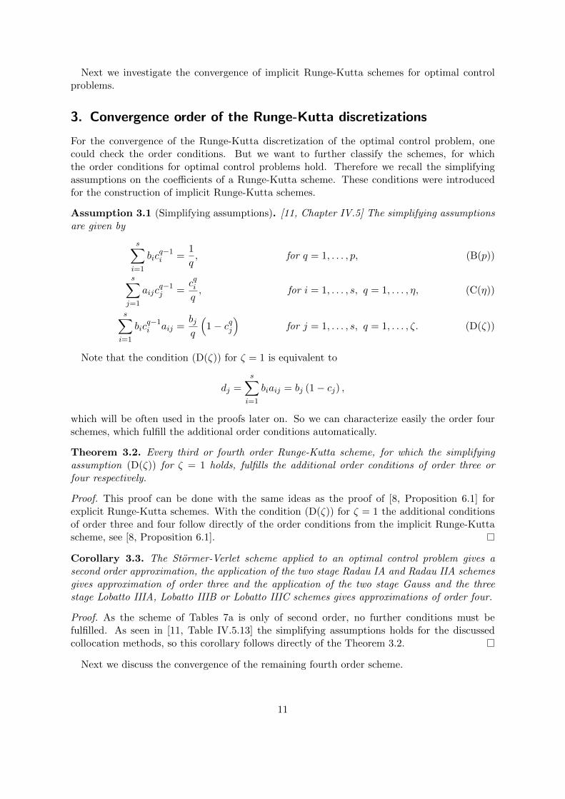
Next we investigate the convergence of implicit Runge-Kutta schemes for optimal controlproblems.

3. Convergence order of the Runge-Kutta discretizations

For the convergence of the Runge-Kutta discretization of the optimal control problem, onecould check the order conditions. But we want to further classify the schemes, for whichthe order conditions for optimal control problems hold. Therefore we recall the simplifyingassumptions on the coefficients of a Runge-Kutta scheme. These conditions were introducedfor the construction of implicit Runge-Kutta schemes.

Assumption 3.1 (Simplifying assumptions). [11, Chapter IV.5] The simplifying assumptionsare given by

s∑i=1

bicq−1i =

1

q, for q = 1, . . . , p, (B(p))

s∑j=1

aijcq−1j =

cqiq, for i = 1, . . . , s, q = 1, . . . , η, (C(η))

s∑i=1

bicq−1i aij =

bjq

(1− cqj

)for j = 1, . . . , s, q = 1, . . . , ζ. (D(ζ))

Note that the condition (D(ζ)) for ζ = 1 is equivalent to

dj =s∑i=1

biaij = bj (1− cj) ,

which will be often used in the proofs later on. So we can characterize easily the order fourschemes, which fulfill the additional order conditions automatically.

Theorem 3.2. Every third or fourth order Runge-Kutta scheme, for which the simplifyingassumption (D(ζ)) for ζ = 1 holds, fulfills the additional order conditions of order three orfour respectively.

Proof. This proof can be done with the same ideas as the proof of [8, Proposition 6.1] forexplicit Runge-Kutta schemes. With the condition (D(ζ)) for ζ = 1 the additional conditionsof order three and four follow directly of the order conditions from the implicit Runge-Kuttascheme, see [8, Proposition 6.1].

Corollary 3.3. The Stormer-Verlet scheme applied to an optimal control problem gives asecond order approximation, the application of the two stage Radau IA and Radau IIA schemesgives approximation of order three and the application of the two stage Gauss and the threestage Lobatto IIIA, Lobatto IIIB or Lobatto IIIC schemes gives approximations of order four.

Proof. As the scheme of Tables 7a is only of second order, no further conditions must befulfilled. As seen in [11, Table IV.5.13] the simplifying assumptions holds for the discussedcollocation methods, so this corollary follows directly of the Theorem 3.2.

Next we discuss the convergence of the remaining fourth order scheme.

11

Theorem 3.4. The pairing of the fourth order SDIRK scheme of Table 8b with the corre-sponding adjoint scheme applied to an optimal control problem provides only a second orderapproximation.

Proof. It is well known that the SDIRK scheme of Table 8b is a fourth order scheme, see [11,Table IV.6.5]. For the falsification of the additional order conditions of order three we see that

s∑i=1

d2i

bi=

18367

588006= 1

3,

and therefore the application to optimal control problem is only of order two, as for order twono additional order conditions are needed.

Remark 3.5. It is easy to check that the schemes of Table 8b and the corresponding adjointscheme are both of order four. Nevertheless the pairing applied to optimal control problems isonly of order two, so we see that the conditions in Table 1c are really additional conditions andare not automatically fulfilled for any implicit Runge-Kutta scheme of the corresponding orderfor ordinary differential equations.

Remark 3.6. The result of Theorem 3.4 is not a general property of SDIRK schemes. Thereare also SDIRK schemes for which in the discretization (3), (4) the convergence order ispreserved, e.g. the SDIRK methods denoted to Crouzeix and Raviart in [11, Exercise IV.6.1],[10, Table II.7.2] of order four with three stages and oder three with two stages.

After the classification of fourth order Runge-Kutta schemes for optimal control, we nowconsider fifth order schemes.

Theorem 3.7. If a Runge-Kutta scheme of order five fulfills the simplifying assumptions(B(p)), (C(η)), (D(ζ)) up to p = 2, η = 2, ζ = 2, then the additional order conditions are alsofulfilled.

Proof. The full proof is given in the Appendix A and done by algebraic manipulation of theadditional order condition with the simplifying assumptions and the usual order conditions.

Corollary 3.8. The three stage Radau IA and Radau IIA implicit Runge-Kutta schemes ap-plied to an optimal control problem are of order five.

Proof. As seen in [11, Table IV.5.13] the schemes fulfill at least the simplifying assumptions(B(p)), (C(η)), (D(ζ)) up to p = 2, η = 2, ζ = 2.

Theorem 3.9. If a Runge-Kutta scheme of order six fulfills the simplifying assumptions(B(p)), (C(η)), (D(ζ)) up to p = 4, η = 2, ζ = 2, then the additional order conditionsare also fulfilled.

Proof. The full proof was carried out by hand by the author by algebraic manipulation of theadditional order condition with the simplifying assumptions and the usual order conditions. Asthis tedious proof gives no higher insights and is, due to the huge number of order conditions,longer as the proof of Theorem 3.7 the details are omitted.

Corollary 3.10. The three stage Gauss and the four stage Lobatto IIIA, Lobatto IIIB andLobatto IIIC implicit Runge-Kutta schemes applied to an optimal control problem are of ordersix.

12

Proof. As seen in [11, Table IV.5.13] the schemes fulfill at least the simplifying assumptions(B(p)), (C(η)), (D(ζ)) up to p = 4, η = 2, ζ = 2.

With Theorem 3.2, Theorem 3.7 and Theorem 3.9 we have sufficient conditions if the addi-tional order conditions are fulfilled which are easy to check. It is open whether these conditionsare also necessary or if there exists an implicit Runge-Kutta scheme which fulfills the additionalorder conditions but not the simplifying assumptions.

Remark 3.11 (Full discretization). In this section the focus was on the time discretizationerror. The full discretization of a parabolic optimal control problem can be handled with themethod of lines as in [1]. Then the error can be split into

‖y(·, ti)− yhi‖L2(Ω) + ‖p(·, ti)− phi‖L2(Ω) . ‖y(·, ti)− yh(ti)‖L2(Ω) + ‖yh(ti)− yhi‖L2(Ω)

+ ‖p(·, ti)− ph(ti)‖L2(Ω) + ‖ph(ti)− phi‖L2(Ω) ,

where the functions yh and ph are discretized in space with a finite element method.

Remark 3.12 (Regularity). The order conditions in this section were taken from [3, 4, 8]and derived with techniques based on Taylor series. Therefore high regularity assumptions andsmooth solutions are needed to observe these rates. For a reduction of the required regularityone might use generalized Taylor polynomials as in the work by Dupont and Scott [5], this iswork of further research.

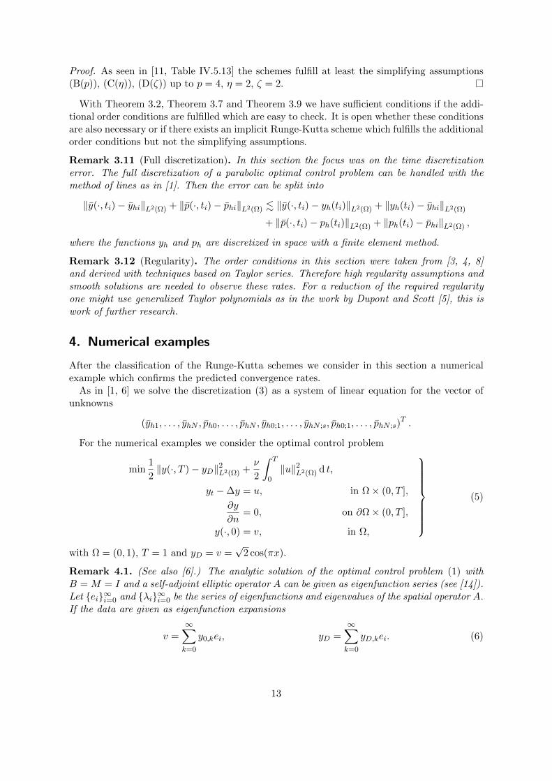
4. Numerical examples

After the classification of the Runge-Kutta schemes we consider in this section a numericalexample which confirms the predicted convergence rates.

As in [1, 6] we solve the discretization (3) as a system of linear equation for the vector ofunknowns

(yh1, . . . , yhN , ph0, . . . , phN , yh0;1, . . . , yhN ;s, ph0;1, . . . , phN ;s)T .

For the numerical examples we consider the optimal control problem

min1

2‖y(·, T )− yD‖2L2(Ω) +

ν

2

∫ T

0‖u‖2L2(Ω) d t,

yt −∆y = u, in Ω× (0, T ],

∂y

∂n= 0, on ∂Ω× (0, T ],

y(·, 0) = v, in Ω,

(5)

with Ω = (0, 1), T = 1 and yD = v =√

2 cos(πx).

Remark 4.1. (See also [6].) The analytic solution of the optimal control problem (1) withB = M = I and a self-adjoint elliptic operator A can be given as eigenfunction series (see [14]).Let ei∞i=0 and λi∞i=0 be the series of eigenfunctions and eigenvalues of the spatial operator A.If the data are given as eigenfunction expansions

v =

∞∑k=0

y0,kei, yD =

∞∑k=0

yD,kei. (6)

13

Table 11: Coefficients for the exact solution (7) of the problem (5) to the data (6).

y0,i yD,i C1,i C2,i C3,i

ai bi−bi+ai e−λi

−2νλi eλi − eλi + e−λi−−bi+ai eλi +2νλiai eλi

−2νλi eλi − eλi + e−λi2λiνC1,i

The optimal control problem decouples into independent problems for every eigenfunction eiand has the solution

y =∞∑i=0

C1,iei eλit +C2,iei e−λit, p =∞∑i=0

C3,iei eλit . (7)

The coefficients can be computed with Maple and are given in Table 11.For the example (5) with yD = v =

√2 cos(πx) the series for the state and the adjoint state

reduce to the terms with the second eigenfunction e1 =√

2 cos(πx) of the Laplace operator withNeumann boundary conditions, i.e. only the coefficients C1,1, C2,1 and C3,1 do not vanish.

The spatial discretization is adapted to the time discretization. The polynomial degree of theLagrange finite elements for the spatial discretization is chosen as k− 1 for time discretizationschemes of order k. So an error splitting argument provides the error bound

‖y(·, ti)− yhi‖L2(Ω) + ‖p(·, ti)− phi‖L2(Ω) . hk + τk.

In the numerical examples the discretization parameters τ and h are chosen so that τ ∼ h.We measure the time discretization error by the quantities

maxi∈0,1,··· ,N

((yhi − Ihy(x, ti))

TM(yhi − Ihy(x, ti))) 1

2 , (8)

maxi∈0,1,··· ,N

((phi − Ihp(x, ti))TM(phi − Ihp(x, ti))

) 12 , (9)

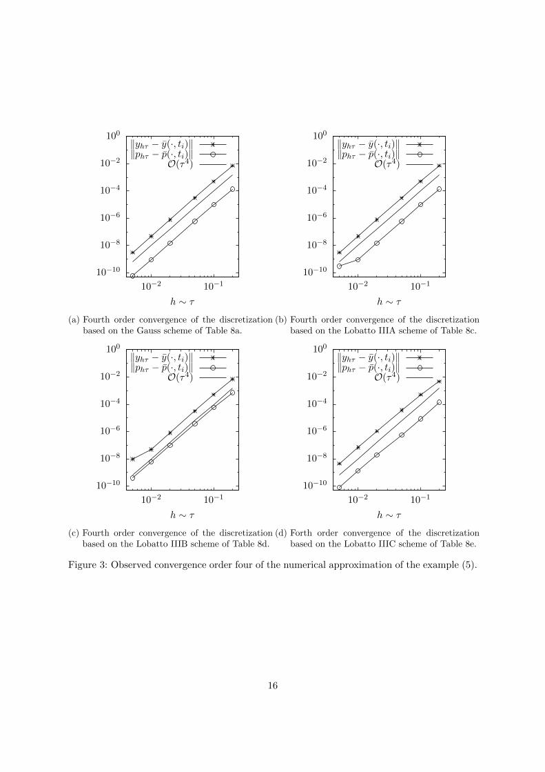
where Ih is the Lagrangian interpolation operator to the corresponding spatial discretizationand M the finite element mass matrix. In Figure 1 to Figure 5 we observe nicely the predictedconvergence rates for the example (5) with ν = 0.001. In the computations with some fourthand sixth order schemes we also observe the influence of the round-off error due to the highnumbers of unknowns. All the computations were done in Matlab.

The predicted order reduction for the SDIRK method can be seen in Figure 1b. For spatialdiscretization of the numerical example with the SDIRK time discretization cubic Lagrangefinite elements are used, as for the other fourth order time discretization schemes.

Remark 4.2. The order reduction of the SDIRK method can also be observed for an optimalcontrol problem with one linear ordinary differential equation. Consider the optimal controlproblem

min1

2(y(1)− 1)2 +

ν

2

∫ 1

0u2 d t,

yt + π2y = u, for t ∈ (0, 1],

y(0) = 1.

(10)

14

10−6

10−5

10−4

10−3

10−2

10−1

100

10−2 10−1

h ∼ τ

‖yhτ − y(·, ti)‖‖phτ − p(·, ti)‖

O(τ2)

(a) Second order convergence of the discretizationbased on the Stormer-Verlet discretization ofTable 7a.

10−6

10−5

10−4

10−3

10−2

10−1

100

10−2 10−1

h ∼ τ

‖yhτ − y(·, ti)‖‖phτ − p(·, ti)‖

O(τ2)

(b) Second order convergence of the discretizationbased on the SDIRK scheme of Table 8b.

Figure 1: Observed convergence order two of the numerical approximation of the example (5).

10−7

10−6

10−5

10−4

10−3

10−2

10−1

100

10−2 10−1

h ∼ τ

‖yhτ − y(·, ti)‖‖phτ − p(·, ti)‖

O(τ3)

(a) Third order convergence of the discretizationbased on the Radau IA scheme of Table 7b.

10−7

10−6

10−5

10−4

10−3

10−2

10−1

100

10−2 10−1

h ∼ τ

‖yhτ − y(·, ti)‖‖phτ − p(·, ti)‖

O(τ3)

(b) Third order convergence of the discretizationbased on the Radau IIA scheme of Table 7c.

Figure 2: Observed convergence order three of the numerical approximation of the example (5).

15

10−10

10−8

10−6

10−4

10−2

100

10−2 10−1

h ∼ τ

‖yhτ − y(·, ti)‖‖phτ − p(·, ti)‖

O(τ4)

(a) Fourth order convergence of the discretizationbased on the Gauss scheme of Table 8a.

10−10

10−8

10−6

10−4

10−2

100

10−2 10−1

h ∼ τ

‖yhτ − y(·, ti)‖‖phτ − p(·, ti)‖

O(τ4)

(b) Fourth order convergence of the discretizationbased on the Lobatto IIIA scheme of Table 8c.

10−10

10−8

10−6

10−4

10−2

100

10−2 10−1

h ∼ τ

‖yhτ − y(·, ti)‖‖phτ − p(·, ti)‖

O(τ4)

(c) Fourth order convergence of the discretizationbased on the Lobatto IIIB scheme of Table 8d.

10−10

10−8

10−6

10−4

10−2

100

10−2 10−1

h ∼ τ

‖yhτ − y(·, ti)‖‖phτ − p(·, ti)‖

O(τ4)

(d) Forth order convergence of the discretizationbased on the Lobatto IIIC scheme of Table 8e.

Figure 3: Observed convergence order four of the numerical approximation of the example (5).

16

10−12

10−10

10−8

10−6

10−4

10−2

100

10−2 10−1

h ∼ τ

‖yhτ − y(·, ti)‖‖phτ − p(·, ti)‖

O(τ5)

(a) Fifth order convergence of the discretizationbased on the three stage Radau IA scheme.

10−12

10−10

10−8

10−6

10−4

10−2

100

10−2 10−1

h ∼ τ

‖yhτ − y(·, ti)‖‖phτ − p(·, ti)‖

O(τ5)

(b) Fifth order convergence of the discretizationbased on the three stage Radau IIA scheme.

Figure 4: Observed convergence order five of the numerical approximation of the example (5).

Even for this very simple example we observe the reduced convergence rate in Figure 6. Againthe regularization parameter ν = 0.001 was chosen.

Remark 4.3. The optimal control problem (10) can be interpreted as a spatial Galerkin dis-cretization of optimal control Problem (5), where the bases of trial and test space are chosen asthe second normalized eigenfunction of the Laplace operator. Note that the first eigenfunctionof the Laplace operator with Neumann boundary conditions is the constant function.

Remark 4.4. In Figure 1a we observe the second order convergence of the Stormer-Verletscheme. Similar observations were presented in [6]. But in contrast to [6], where the conver-gence of the state was observed in the time discretization points ti and the convergence of theadjoint state was observed in the time middle points ti+ 1

2= ti+ti+1

2 , we present in Figure 1a

the convergence of the state and the adjoint state in the time discretization points ti.

5. Conclusions and Outlook

In this paper we discussed the use of higher order implicit Runge-Kutta schemes for optimalcontrol with parabolic partial differential equations for which optimization and discretizationcommute. In terms of the well known simplifying assumptions on the coefficients of implicitRunge-Kutta scheme we were able to give a classification for which discretization schemesup to order six the convergence order is preserved. For collocation schemes of Gauss, RadauIA, Radau IIA, Lobatto IIIA, Lobatto IIIB and Lobatto IIIC type and a SDIRK scheme theexpected and the numerical convergence rates coincide nicely.

For schemes of order higher than six the order conditions are not known explicitly, butthey can be computed with the aid of bi-colored Butcher trees, as described in [3, 4]. For areduction of the additional order conditions of order higher as six the procedure presented in

17

10−12

10−10

10−8

10−6

10−4

10−2

10−2 10−1

h ∼ τ

‖yhτ − y(·, ti)‖‖phτ − p(·, ti)‖

O(τ6)

(a) Sixth order convergence of the discretizationbased on the three stage Gauss scheme.

10−12

10−10

10−8

10−6

10−4

10−2

10−2 10−1

h ∼ τ

‖yhτ − y(·, ti)‖‖phτ − p(·, ti)‖

O(τ6)

(b) Sixth order convergence of the discretizationbased on the four stage Lobatto IIIA scheme.

10−12

10−10

10−8

10−6

10−4

10−2

10−2 10−1

h ∼ τ

‖yhτ − y(·, ti)‖‖phτ − p(·, ti)‖

O(τ6)

(c) Sixth order convergence of the discretizationbased on the four stage Lobatto IIIB scheme.

10−12

10−10

10−8

10−6

10−4

10−2

10−2 10−1

h ∼ τ

‖yhτ − y(·, ti)‖‖phτ − p(·, ti)‖

O(τ6)

(d) Sixth order convergence of the discretizationbased on the four stage Lobatto IIIC scheme.

Figure 5: Observed convergence order six of the numerical approximation of the example (5).

18

10−10

10−8

10−6

10−4

10−2

100

102

10−4 10−3 10−2 10−1

τ

‖yhτ − y(·, ti)‖‖phτ − p(·, ti)‖

O(τ2)

Figure 6: Observed convergence for example (10) with the SDIRK method.

this paper is not practical due the huge number of additional conditions. Therefore a moreelegant technique should be developed for the classification of schemes of order higher thansix.

Acknowledgements

The work was partially supported by the DFG priority program SPP 1253.

A. Proof of Theorem 3.7

Full proof of Theorem 3.7. The idea of the proof is to use the simplifying assumptions (B(p)),(C(η)), (D(ζ)) to reduce the additional order conditions to the classic order conditions or orderconditions of lower order, which have already been reduced to the order conditions of the un-controlled system. As all the numerical schemes fulfill the order conditions for the uncontrolledsystems, these conditions can be used to calculate the value of the reduced expression.

Surely the way of the application of the simplifying assumptions is not unique, here onepossibility is presented. A first goal in the reduction of order conditions with a fraction ·

biis

to use (D(ζ)) to produce an additional bi which cancels out. In the following we discuss thereduction of all the additional order conditions.

1. For the first additional order condition of (A5-1) we use the simplifying assumption(D(ζ)) for ζ = 1, the last condition of (O4) and the first condition of (O5-3). This yields∑

kl

1

bkalkckdkdl =

∑kl

dlalkck −∑kl

alkc2kdl =

1

24− 1

60=

1

40.

2. For the second additional order condition of (A5-1) we use the simplifying assumption(D(ζ)) for ζ = 1 and the third condition of (O4) and the second condition of (O5-3) to

19

get ∑k

1

bkc2kd

2k =

∑k

c2kdk −

∑k

c3kdk =

1

12− 1

20=

1

30.

3. For the last order condition of (A5-1) we use again the simplifying assumption (D(ζ))for ζ = 1, the first condition of (O3) the third condition of (O4) and the first conditionof (O5-2). This gives∑

l

1

b2lcld

3l =

∑cldl − 2

∑c2l dl +

∑l

c3l dl =

1

6− 2

12− 1

20=

1

20.

4. For the first condition of (A5-2) we apply the simplifying assumption (D(ζ)) for ζ = 1and use the last condition of (O4) and the second condition of (O5-1), which gives∑

kl

1

bkaklcld

2k =

∑kl

aklcldk −∑kl

aklcldkck =1

24− 1

40=

1

60.

5. For the second condition of (A5-2) we use the simplifying assumption (D(ζ)) for ζ = 1,the condition (O2), the first condition of (O3), the third condition of (O4) and the firstcondition of (O5-2) to end with∑

m

1

b3md4m =

∑m

dm −∑m

3dmcm +∑m

3dmc2m −

∑m

dmc3m =

1

5.

6. For the third condition of (A5-2) we apply the simplifying assumption (C(η)) for η = 2twice and get with the second condition of (O5-3) the result

∑ijk

biaikaijcjck =∑i

bi

(∑k

aikck

)∑j

aijcj

=1

4

∑i

bic4i =

1

20.

7. For the first condition of (A5-3) we apply again the simplifying assumption (C(η)) forη = 2 and the use of the first condition of (O5-3) yields

∑jkl

alkakjcjdl =∑kl

alkdl

∑j

akjcj

=1

2

∑kl

alkdlc2k =

1

120.

8. For the second condition of (A5-3) we apply first the simplifying assumptions (D(ζ)) forη = 1 and then the definition of cl and the simplifying assumption (C(η)) for η = 2.Together with the third condition of (O4) and the first condition of (O5-2) this gives

∑kl

1

bkalkdkcldl =

∑l

cldl

(∑k

alk

)−∑l

cldl

(∑k

alkck

)=∑l

c2l dl −

1

2

∑l

c3l dl =

7

120.

20

9. For the last condition of (A5-3) we apply the simplifying assumption (D(ζ)) for η = 2twice and get with (O1), the second condition of (O2) and the second condition of (O5-3)the result

∑ijk

bibjbk

ajkaikcicj =∑jk

bjbkajkcj

(∑i

biaikci

)=

1

2

∑k

(1− ck)

∑j

bjajkcj

=

1

4

∑k

bk(1− ck)(1− c2k) =

1

4

∑k

(bk − 2bkc

2k + bkc

4k

)=

2

15.

10. For the first condition of (A5-4) we use the simplifying assumption (D(ζ)) for η = 1and η = 2, the second condition of (O4), the second condition of (O3) and the secondcondition of (O5-3) to get

∑ik

bibkaikcickdk =

∑ik

biaikcick −∑

c2k

(∑i

biciaik

)=

1

8− 1

2

∑c2kbk(1− c2

k

)=

7

120.

11. For the second condition of (A5-4) we use again the simplifying assumptions (D(ζ)) forη = 1 and η = 2. The remaining expressions are treated with (O1), the simplifyingcondition (B(p)) for p = 2, the second condition of (O3), the first condition of (O4) andthe second condition of (O5-3). This gives

∑il

bib2lailcid

2l =

∑il

biailci(1− cl)2 =∑l

(1− cl)2

(∑i

biciail

)=

1

2

∑l

bl(1− cl)2(1− c2l )

=1

2

∑l

(bl − 2blcl + 2blc

3l − blc4

l

)=

3

20.

12. For the last condition of (A5-4) we use first the simplifying assumptions (D(ζ)) for η = 1we get due to symmetry properties∑lmk

1

bkamkalkdldm =

∑lmk

blbmbk

amkalk(1− cl)(1− cm)

=∑lmk

blbmbk

amkalk − 2∑lmk

blbmbk

amkalkcl +∑lmk

blbmbk

amkalkclcm. (11)

The last term is the third condition of (A5-3) and therefore we already know how totread this term. On the first term of (11) we apply the simplifying assumptions (D(ζ))for η = 1 twice and get with (O1), (B(p)) for p = 2 and the second condition of (O3)

∑lmk

blbmbk

amkalk =∑k

1

bk

(∑m

bmamk

)(∑l

blalk

)=∑k

bk(1− ck)2 =1

3.

For the remaining term of (11) the use of (D(ζ)) for η = 1 and η = 2 and (O1), (B(p))for p = 2, the second condition of (O2) and the first condition of (O2) yields

∑lmk

blbmbk

amkalkcl =∑k

1

bk

(∑m

bmamk

)(∑l

blalkcl

)=

1

2

∑k

bk(1− ck)(1− c2k) =

5

24.

21

Altogether we have ∑lmk

1

bkamkalkdldm =

1

3− 5

12+

2

15=

1

20.

13. For the first condition of (A5-5) we start with the use of the simplifying assumption(D(ζ)) for η = 1 and the definition of cm. The last condition of (O4), the first conditionof (O5-3) and the first condition of (O3) give∑

lm

1

b2lamld

2l dm =

∑lm

aml(1− cl)2dm =∑lm

amldm − 2∑lm

amlcldm +∑lm

amlc2l dm

=∑m

cmdm −1

12+

1

60=

1

6− 1

15=

1

10.

14. For the second condition of (A5-5) the use of (D(ζ)) for ζ = 1, the definition of ci, thelast condition of (O4), the simplifying assumption (C(η)) for η = 2 and the first conditionof (O5-3) yields∑

kml

1

bkamlalkdkdm =

∑kml

amlalkdm −∑kml

amlalkdmck

=∑ml

amlcldm −∑ml

amldm

(∑k

alkck

)=

1

24− 1

2

∑ml

amldmc2l

=1

24− 1

120=

1

30.

15. For the last condition of (A5-5) we apply the simplifying assumption (D(ζ)) for ζ = 2,the definition of cl, first condition of (O5-3) and the first condition of (O3) to get

∑ilk

bibkalkaikcidl =

∑lk

1

bkalkdl

(∑i

biaikci

)=

1

2

∑lk

alkdl −1

2

∑lk

alkdlc2k

=1

2

∑l

cldl −1

120=

3

40.

16. For the first condition of (A5-6) we use the simplifying assumption (D(ζ)) for ζ = 1 andthe simplifying assumption (C(η)) for ζ = 2 three times. With the definition of ci, thefirst condition of (O4) and the second condition of (O5-3) we get

∑ikl

bibkaikaildkcl =

∑ik

biaik

(∑l

ailcl

)−∑i

bi

(∑k

aikck

)(∑l

ailcl

)

=1

2

∑i

bic2i

(∑k

aik

)− 1

4

∑i

bic4i =

1

2

∑i

bic3i −

1

20=

1

8− 1

20=

3

40.

17. To the second condition of (A5-6) we apply the simplifying assumption (D(ζ)) for ζ = 1once, use the definition of ci, the third condition of (A4) and the first condition of (A5-6).

22

This yields ∑ilm

biblbm

aimaildldm =∑ilm

bibmaimaildm −

∑ilm

bibmaimailcldm

=∑ilm

bibmaimcldm −

∑ilm

bibmaimailcldm =

2

15.

18. The application of the simplifying assumption (D(ζ)) for ζ = 1 to the last conditionof (A5-6) together with the last condition of (O5-2), the definition of ci and the firstcondition of (O4) gives∑

ik

bibkaikc

2i dk =

∑ik

biaikc2i −

∑ik

biaikc2i ck =

∑ik

bic3i −

1

10=

3

20.

19. For the condition (A5-7) we use the simplifying assumption (D(ζ)) for ζ = 1 two times,the definition of cl, the first condition of (O3), the third and fourth conditions of (O4)and the second condition of (O5-1) and get∑

lm

1

blbmalmd

2l dm =

∑lm

almdl −∑lm

almdlcl −∑lm

almdlcm +∑lm

almdlclcm

=∑lm

cldl −∑lm

c2l dl −

∑lm

almdlcm +∑lm

almdlclcm =1

15

Altogether we have derived the additional order conditions with the use of the simplifyingassumptions and (B(p)) for p ≤ 2, (C(η)) for η = 1, 2, (D(ζ)) for ζ = 1, 2, and the orderconditions (O1)–(O4) and (O5-1)–(O5-3).

References

[1] Thomas Apel and Thomas G. Flaig. Crank-Nicolson schemes for optimal control problemswith evolution equations. SIAM Journal on Numerical Analysis, 50(3):1484–1512, 2012.

[2] Roland Becker, Dominik Meidner, and Boris Vexler. Efficient Numerical Solution ofParabolic Optimization Problems by Finite Element Methods. Optimization Methodsand Software, 22(5):813 – 833, 2007.

[3] J. Frederic Bonnans and Julien Laurent-Varin. Computation of order conditions for sym-plectic partitioned Runge-Kutta schemes with application to optimal control. Rapport derecherche RR–5398, INRIA, http://hal.inria.fr/docs/00/07/06/05/PDF/RR-5398.

pdf, 2004.

[4] J. Frederic Bonnans and Julien Laurent-Varin. Computation of order conditions for sym-plectic partitioned Runge-Kutta schemes with application to optimal control - Order con-ditions for symplectic partitioned Runge-Kutta schemes (second revision). NumerischeMathematik, 103:1–10, 2006.

[5] Todd Dupont and Ridgway Scott. Polynomial approximation of functions in Sobolevspaces. Mathematics of Computation, 34(150):441–463, 1980.

23

[6] Thomas G. Flaig. Discretization strategies for optimal control problems with parabolicpartial differential equations. PhD thesis, Universitat der Bundeswehr Munchen, 2013.

[7] William W. Hager. Rates of convergence for discrete approximations to unconstrainedcontrol problems. SIAM Journal on Numerical Analysis, 13(4):449–472, 1976.

[8] William W. Hager. Runge-Kutta methods in optimal control and the transformed adjointsystem. Numerische Mathematik, 87:247–282, 2000.

[9] Ernst Hairer, Christian Lubich, and Gerhard Wanner. Geometric Numerical Integration:Structure-Preserving Algorithms for Ordinary Differential Equations. Springer-Verlag,Berlin, second edition, 2006.

[10] Ernst Hairer, Syvert Paul Nørsett, and Gerhard Wanner. Solving Ordinary DifferentialEquations I. Nonstiff Problems. Springer-Verlag, Berlin, 1987.

[11] Ernst Hairer and Gerhard Wanner. Solving Ordinary Differential Equations II. Stiff andDifferential-Algebraic Problems. Springer-Verlag, Berlin, 2nd revised edition, 1996.

[12] Michael Herty, Lorenzo Pareschi, and Sonja Steffensen. Implicit-explicit runge-kuttaschemes for numerical discretization of optimal control problems. SIAM Journal on Nu-merical Analysis, 51(4):1875–1899, 2013.

[13] Michael Herty, Lorenzo Pareschi, and Sonja Steffensen. Numerical methods for the optimalcontrol of scalar conservation laws. In Dietmar Homberg and Fredi Troltzsch, editors,System modeling and Optimization, 25th IFIP TC7 Conference, CSMO 2011, Berlin,Germany, September 12-16, 2011, Revised Selected Papers. Springer, Heidelberg, 2013.

[14] L. Steven Hou, Oleg Imanuvilov, and Hee-Dae Kwon. Eigen series solutions to terminalstate tracking optimal control problems and exact controllability problems constrained bylinear parabolic PDEs. Journal of Mathematical Analysis and Applications, 313:284–310,2006.

[15] Jens Lang and Jan G. Verwer. W-Methods in optimal control. Numerische Mathematik,124:337–360, 2013.

[16] P. Lasaint and P.-A. Raviart. On a finite element method solving the neutron transportequation. In Carl de Boor, editor, Mathematical aspects of finite elements in partialdifferential equations. Academic Press, New York, 1974.

[17] Jacques Louis Lions. Optimal Control of Systems Governed by Partial Differential Equa-tions. Springer, Berlin, 1971.

[18] Dominik Meidner and Boris Vexler. A Priori Error Estimates for Space-Time FiniteElement Discretization of Parabolic Optimal Control Problems. Part I: Problems withoutControl Constraints. SIAM Journal on Control and Optimization, 47(3):1150 – 1177,2008.

[19] Dominik Meidner and Boris Vexler. A priori error analysis of the Petrov Galerkin CrankNicolson scheme for parabolic optimal control problems. SIAM Journal on Control andOptimization, 49(5):2183 – 2211, 2011.

24

[20] Arnd Rosch. Error estimates for parabolic optimal control problems with control con-straints. Zeitschrift fur Analysis und ihre Anwendungen, 23(2):353–376, 2004.

[21] Fredi Troltzsch. Optimale Steuerung partieller Differentialgleichungen - Theorie, Ver-fahren und Anwendungen. Vieweg, Wiesbaden, 2005.

25