Implied Cost of Equity Capital in Earnings-based Valuation: International Evidence

ABSTRACT Assuming the clean surplus relation, the Edwards-Bell-Ohlson residual income valuation (RIV)

model expresses market value of equity as the sum of the book value of equity and the expected

discounted future residual incomes. Without assuming clean surplus, Ohlson and Juettner-

Nauroth (2000) show that the forward earnings per share are critical for valuation. We compare

the implied costs of capital from these two approaches to earnings-based valuation for seven

developed countries. We hypothesize superior performance from the RIV model in countries

where analysts’ forecasts of dividends, earnings, and book values of equity conform well to clean

surplus. First, we provide preliminary international evidence on the frequency and magnitude of

clean surplus violations. Second, we document, consistent with our hypothesis, that the implied

cost of capital is more reliable when derived from the RIV model when clean surplus adequately

describes the firms’ financial reporting. That is, the implied cost of capital derived from Ohlson

and Juettner-Nauroth (2000) is relatively more reliable in countries where clean surplus

deviations are common. Our analyses suggest that the proper choice of earnings-based valuation

model may depend on analysts’ interpretation of their financial reporting environment.

0

Implied Cost of Equity Capital in Earnings-based Valuation: International Evidence

1. Introduction

As is now well understood, the Edwards-Bell-Ohlson residual income valuation model

(hereafter RIV model) requires the clean surplus relation to rewrite the dividend discount model.

In this paper, we provide initial evidence of how the assumption of the clean surplus relation

applies to accounting data for firms in different countries. We proceed to investigate whether the

performance of the RIV model varies internationally with how well the assumption of the clean

surplus relation fits each country. As argued below, we predict that in reporting environments

where analyst forecasts of firms’ future performance in accounting terms consistently violate the

clean surplus relation, the RIV model is less likely to succeed. As a benchmark for our analysis,

we consider the Ohlson and Juettner-Nauroth model (hereafter OJ model) which does not assume

that clean surplus relation holds. We examine the relative reliability of the implied costs of

equity from two earnings-based approaches, the RIV valuation model and the OJ model, within a

sample of seven developed countries.

That most prior empirical analyses use data from U.S. stock markets might raise

methodological concerns. The capital markets around the world are, from the perspective of

investors and analysts, either integrated or segmented. Suppose initially that capital markets are

largely integrated on a global scale. First, analysts in different countries likely apply different

heuristics to process their information and generate earnings forecasts. For example, the use of

PEG ratios, which are a special case of the OJ model, is documented in the U.S. starting in the

1

early 1990s, but its use has not been documented internationally.1 The representativeness of any

single valuation model, such as PEG ratios, and the variation in analysts’ choice of valuation

methods might differ between stock markets and countries. Second, since the U.S. economy has

been growing consistently over a prolonged period of time, the inferred growth rates might be

overstated relative to the average growth rate of the world. Alternatively, suppose that capital

markets are segmented and that investors’ portfolio choices exhibit home bias. In that case, the

inferences drawn from the performance of any single country might not generalise to other

markets.

First, take as given that we wish to provide evidence on the clean surplus relation in

international accounting data. While differences in accounting methods and in analysts’ use of

information remain across firms within any single country, this variation is likely more

pronounced globally. We provide two types of evidence, ex ante and ex post. First, we provide

evidence on the properties of analyst forecasts. We selected a sample of firms for which analysts

make three forecasts available: book values of equity, earnings, and dividends. For this

particular sample, we establish that analysts’ forecasts do not adhere to the clean surplus relation.

Thus, the clean surplus relation may not be an equally effective assumption in all countries.

Consistent with analysts forming rational expectations, the clean surplus relation need not be a

descriptive assumption in financial reporting environments where the accounting standards allow

or require material deviations from the clean surplus relation. To investigate this possibility, we

proceeded to analyze the ex post performance of book value of equity, earnings, and dividends.

Following Lo and Lys (2001), we provide evidence on the magnitude of deviations from the

clean surplus relation in percentage of the ending book value of equity. Such deviations from the 1 See Bradshaw (2002, 2004). We performed an unstructured search of the Internet and found examples of PEG ratios in France (Paris-based analyst Arnaud Joly on Mr. Bricolage SA in 2002), Germany (MediClin) and the U.K. (Phillip Securities Limited on Barclays PLC).

2

clean surplus relation in prior years could, if correlated with analyst forecasts deviations from

clean surplus, impact the precision of our estimated costs of capital.2

Second, producing a reliable empirical representation of firms’ expected cost of equity is, of

course, a fundamental accounting research question in its own right. Early research discovered

that ex post realised stock return is a natural, but noisy and potentially biased, proxy of the

expected cost of equity (Elton, 1999). For example, Gebhardt, Lee, and Swaminathan (2001)

analyze the expected cost of equity implied in the equation between stock prices and intrinsic

value estimates based on analyst earnings forecasts. In this paper, we are interested in what type

of earnings-based valuation models, RIV or OJ, should be used in different countries.

Although the earnings-based valuation models derive from a common underlying theory,

the dividend discount valuation, their empirical implementation may cause differences in their

assessed validity. When the empirical implementation involves simplifying assumptions about

dividend payout ratios or terminal value calculations, the reliability in the implied cost of equity

may decrease. Therefore, which valuation model is preferred for deriving a reliable implied cost

of equity is an empirical question. However, given the plethora of possible implementations, this

question is difficult to resolve exhaustively. We address this concern by undertaking the

representative implementations of alternative valuation models to different environments.

We extend prior studies of the implied cost of equity into an international setting,

examining the reliability of the implied costs of equity both in general and in specific

environment. We consider the implied costs of equity derived from the representative earnings-

based valuation models, such as the OJ model, the PEG model, and two different

implementations of RIV models, within Australia, Canada, France, Germany, Japan, the U.K.

2 The implied cost of equity capital resulting from implementation of RIV models without a terminal value assumption should be unaffected by ex post deviations from clean surplus. See formal proof in the appendix.

3

and the U.S. These seven countries were chosen because they cover a substantial proportion of

the world’s total stock market capitalization with data available.

Diverse accounting standards and economic situations across seven countries offer an

empirical setting, in which we can examine the robustness of the relative reliability of alternative

estimates of implied costs of equity. For example, if a specific assumption about terminal values

is descriptive of the underlying economic reality, the resulting implied cost of equity can

approximate the true, unobservable cost of equity. Since seven countries are under different

economic and regulatory conditions, our international study facilitates more robust inferences

about the relative reliability of the implied cost of equity. In particular, cross-country variation

in dirty surplus accounting should affect the RIV model, but not the OJ model.3 As already

argued, the theoretical advantage of the OJ model is that it avoids the assumption of the clean

surplus relation, while the RIV model requires it. This difference motivates testing the relative

reliability of the implied cost of equity based on the OJ model versus the RIV model.

We examine which implied cost of equity is more closely associated with the representative

risk proxies within each country and then compare the relative ranks of implied cost of equity

across countries. Specifically, our metric of the reliability of the implied cost of equity is the

adjusted 2R of the regression of implied cost of equity on common risk proxies. In addition, we

examine the individual correlation between implied cost of equity and risk proxies as a

supplementary metrics.

In terms of the association with risk proxies, we find that the RIV model reflecting industry-

specific information is superior to, or equivalent with, alternative implementation of the RIV

model that only reflects firm-specific information. That is, industry-specific information is

3 This is in the spirit of Walker (1997, p.352).

4

incrementally helpful for enhancing the implied costs of equity for our countries. Further, the OJ

model appears inferior to, or equivalent with, the PEG model (a simpler version of the OJ model),

in all countries. Finally, we find that the RIV model clearly dominates the OJ model in countries

where clean surplus tends to hold (Australia, Canada, Japan and U.S.) which is not the case for

the European countries which exhibit more pronounced dirty surplus. Overall, the clean surplus

relation affects the relative performance of the RIV model as we predict.

Our study makes several contributions to the existing literature. We evaluate different

measures of the implied costs of equity based on the RIV model and the OJ model in an

international setting. Although prior research has examined the relative reliability of alternative

implied costs of equity using the U.S. data, it remains unresolved whether these results

generalise to other countries. By exploiting the diversity of economic conditions and accounting

rules across seven countries, we offer more robust conclusions regarding to the relative reliability

of implied costs of equity. Second, increasingly globalised financial markets motivate investors

and analysts interest in which valuation model to use for the implied costs of equity. Third, the

fact that the potential violation of the clean surplus relation affects the relative validity of

accounting-based valuation models might inspire accounting standard setters in different

countries as they decide whether to pursue the reporting of the comprehensive income.

The paper proceeds as follows. Section 2 reviews the related literature. Sections 3 and 4

describe the variable measurements and our sample. We present our empirical evidence in

Section 5 and summarize in Section 6.

5

2. Literature Review

Our research relates to the intersection between the implied cost of equity and the

international valuations. This section briefly outlines the literatures in these areas.

2.1 Prior Literature on Implied Cost of Equity

Research in accounting and finance explored the ex ante cost of equity which is required as

input for tests of asset pricing models and accounting-based valuation models. Since the ex ante

cost of equity is unobservable, ex post realised stock returns are an often-used proxy. The ex

post return has proven a notoriously noisy proxy for the ex ante cost of equity (for example, see

Fama and French, 1997).

Gebhardt et al. (2001) present an alternative approach to estimating the ex ante cost of

equity by calculating the internal rate of return that equates the stock prices with the intrinsic

value estimates based on analyst earnings forecasts. They calculate the implied cost of equity

from the RIV model using analyst earnings forecasts as proxies of the market’s earnings

expectations. Gebhardt et al. (2001) proceed to examine the relation between these implied costs

of equity and ex ante firm characteristics previously suggested as risk proxies. They conclude

that the implied cost of equity is systematically correlated with several risk proxies, suggesting

the reasonableness of their alternative approach to estimate the ex ante cost of capital.

Subsequent papers examine the reliability of the alternative implied costs of equity. For

example, Botosan and Plumlee (2002) assess which valuation model produces the implied cost of

equity approximating the ex ante cost of equity. They conclude that the implied cost of equity

derived from the PEG model associates consistently with all of the considered risk proxies. In

contrast, the associations between the implied cost of equity based on the RIV model or the OJ

model and their risk proxies are unstable. Similarly, Easton and Monahan (2003) provide

6

evidence that the implied cost of equity derived from naïve heuristics, such as price-to-forward

earnings multiple, are as reliable as those derived from theoretical models, such as the RIV

model or the OJ model. However, U.S.-based results reported by Gode and Mohanram (2003)

include that the RIV model reflecting industry-specific information outperforms the OJ model in

terms of the correlations with risk proxies. Guay, Kothari, and Shu (2003) conclude that only the

implied cost of equity derived from the RIV model reflecting industry-specific information

exhibits a significant correlation with two-year and three-year-ahead stock returns.

In summary, although prior research examines the reliability of implied costs of equity

derived from a variety of valuation models in terms of the association with frequently cited risk

proxies or realised stock returns, their analysis is generally limited to U.S. firms. Further, their

conclusions regarding the relative reliability of implied costs of equity remain mixed.

2.2 Prior Literature on International Valuation

Despite the popularity of the RIV model, with the exception of Frankel and Lee (1999),

little research explores the performance of the RIV model, or OJ model, in an international

setting. Frankel and Lee (1999) conclude that firm value estimates derived from the RIV model

adequately explains the cross-sectional distribution of the stock prices in 20 countries. They find

that, in most countries, the intrinsic value estimates based on the RIV model account for more

than 70% of the cross-sectional variation of stock prices. Their results predict that the implied

cost of equity derived from the RIV model might be reliable within their sample countries.

Of particular interest for this study, Frankel and Lee (1999) point to the possibility that

systematic violations of the clean surplus relation as a source of noise in the intrinsic value

estimates based on analyst earnings forecasts. This would imply that the country-specific extent

of the clean surplus relation violation might affect the relative reliability of the implied costs of

7

equity derived from the RIV model or from the OJ model across countries. Given the limited

evidence on the relative validity of different earnings-based valuation models across countries,

we provide initial evidence on cross-country variation in the degree of clean surplus violations.

3. Research Design and Variable Measurement

This section describes how we compare the reliability of different implied costs of equity,

the assumptions we apply to different valuation models to derive the implied costs of equity, and

which variables are chosen as the representative risk proxies.

3.1 Measurement of the Reliability of Implied Cost of Equity

Since the true ex ante cost of equity is unobservable, a direct assessment of the reliability of

implied cost of equity is not possible. However, an indirect way of assessment is to examine the

relationships between the implied cost of equity and the risk proxies that are believed to affect

the cost of equity. We base our empirical specification of risk premia in the capital markets on

the Arbitrage Pricing Theorem (APT). Ross (1976) derives firm i ’s expected cost of equity

( [ ]iE r ) is a function of the risk free rate ( fr ) and the excess expected return associated with K

risk factors. This leads to the following equation for the expected cost of equity:

[ ] [ ]( )1

K

i f k k fk

E r r E r rλ=

= + −∑ (1)

While this APT does not identify the risk factors, prior research identified risk proxies, described

below, which we use in this study.

Based on equation (1), we examine which implied costs of equity are more highly

associated with our risk proxies in cross-section within each country.4 If a specific implied cost

4 This methodology is consistent with Gebhardt et al. (2001), Botosan and Plumlee (2002) and Gode and Mohanram (2003).

8

of equity is more reliable than others, this estimate should exhibit a stronger association with risk

proxies. Therefore, we use the adjusted 2R of the regression of implied cost of equity on

frequently cited risk proxies as the main metric of the reliability of the implied cost of equity. In

addition, we examine the individual correlation between implied cost of equity and risk proxies

as a supplementary metric.

3.2 Alternative Measures of Implied Cost of Equity

We derive the implied cost of equity using the OJ model and the PEG model (a specific

form of the OJ model) as well as two implementations of the RIV model. We compute the

implied cost of equity for each firm as the internal rate of return that equates the stock prices to

intrinsic value estimates based on one-year-ahead and two-year-ahead earnings forecasts.5 All of

the four methods we examine are derived from same underlying valuation model, i.e., the

dividend discount model.

( )1 1t n

t t nn t

dP Er

∞+

=

=

+ ∑ (2)

where is the stock price at period t, d are the dividends net of capital contributions during

period t, and is the firm’s cost of equity.

tP t

tr

However, the RIV model specifies the valuation using the ‘return on equity’ rather than the

level of ‘abnormal earnings’ as in the OJ model. Furthermore, the implementations of even the

same valuation model differ mainly in their assumptions about the forecasts horizon and the

5 Since analyst forecasts of five-year earnings growth are not available for many of foreign firms, we use only one- and two-year-ahead earnings forecasts under a specific assumption about the longer period ahead earnings. In this study, this implementation is sensible since our implementation of the OJ model use only one- and two-year-ahead analyst earnings forecasts and so the comparison between the OJ model and the RIV model is not affected by the different usage of analyst earnings forecasts for different horizons. Frankel and Lee (1999) also use only one- and two-year-ahead analyst earnings forecasts in their international valuation study. Furthermore, Lo and Lys (2001) indicate that to reflect long-term analyst earnings forecasts into the RIV model does not significantly improve its pricing performance.

9

earnings growth after forecasts horizon. For example, the OJ model uses economy-wide

assumptions for the terminal earnings growth, while an implementation of the RIV model

incorporates industry-specific assumptions for the terminal earnings growth. These differences

in implementation might affect the reliability of the implied cost of equity. The remaining part

of this section describes the salient features and key assumptions underlying these four

implementations.

3.2.1 The Residual Income Valuation Model

According to the RIV model (Ohlson, 1995), intrinsic values can be expressed as the

reported book value of equity plus an infinite sum of discounted residual income, as long as the

dividend discount model is descriptive of equilibrium prices and clean surplus accounting is

followed. However, the empirical implementation of the RIV model requires additional

assumptions about forecast horizon, terminal value calculation, dividend payout ratios as well as

the explicit forecasts of future ROE before forecast horizon. We forecast future ROE explicitly

for the next two years using analyst earning forecasts, and then forecast ROE beyond year t+2

implicitly by adopting different terminal value calculations used in prior representative studies

using the RIV model.

Following the prior research, we estimate the implied cost of equity from two

implementations of the RIV model. The two implementations differ only in their assumptions

about the forecasts horizon and the growth of residual income beyond the forecasts horizon.

Following Frankel and Lee (1998), Lee Myers, and Swaminathan (1999), Liu, Nissim, and

Thomas (2002), and Ali, Hwang, and Trombley (2003), our first RIV model (hereafter RIVC)

assumes that the residual income is constant beyond year t 2+ . For each period t, we denote

earnings by and book value of equity by bv such that: teps t

10

21 2

21

( ) ((1 ) (1 )

t t s t t s t t t tt t s

s t t

E eps r bv E eps r bvP bvr r

+ + − +

=

− × − ×= + + + ×

∑ 1)

tr+

+ (3)

Our second RIV model (hereafter RIVI) assumes that the ROE trends linearly to the

industry median ROE by the 12th year and that thereafter the residual incomes remain constant in

perpetuity.6 The industry median ROE is calculated by the moving median of the previous five

years’ ROE of the firms within the same industry.7 Following Gebhardt et al. (2001), only firms

with positive ROE are used in the calculation. The assumption of the future ROE’s conversion

toward the industry median ROE is consistent with Lee et al. (1999), Gebhardt et al. (2001) and

Liu et al. (2002).

2 111 1

111 3

( ) [ ( )] [ ( )]

(1 ) (1 ) (1 )t t s t t s t t s t t s t t t t

t t s ss st t t

12 11

t

E eps r bv E ROE r bv E ROE r bvP bv

r r r+ + − + + − +

= =

− × − × − ×= + + +

+ + ×

∑ ∑r

+

+ (4)

where tROE is the return on equity during period t.

As stated previously, the RIVI model reflects the industry-specific information into terminal

value calculation while the RIVC model does not. Therefore, if long-term industry performance

is an important determinant of the valuation, the implied cost of equity derived from the RIVI

model will be superior to the implied cost of equity derived from the RIVC model.

Lastly, we make the same assumptions about dividend payout ratio to both models as

follows. If analyst forecasts of dividends are available, we apply those forecasts as future

dividends. When analyst forecasts of dividends are not available, we estimate future dividend

payout ratio by scaling dividends in the most recent year by earnings over the same year. For the

firms with negative earnings, we divide dividends in the most recent year by one-year-ahead or

two-year-ahead analyst earnings forecast to derive an estimated payout ratio. If both earning 6 See Myers (1999) for a discussion on intertemporal consistency 7 Since the data is limited for international firms, we use the median of the prior five years. We use the most general I/B/E/S industry classification, ‘Sector’, when calculating the industry median of ROE.

11

forecasts are still negative, we assume the future dividend payout ratio to be zero. If the

estimated dividend payout ratio is larger than 0.5, we assume the payout ratio to be 0.5. We

compute future book values of equity using the dividend forecasts (if not available, dividend

payout ratio) and analyst earnings forecasts based on the clean surplus relation.

Under these assumptions, we solve for r by searching over the range of 0 to 100% for a

value of r that minimises the difference between the stock prices and the intrinsic value

estimates based on analyst earnings forecasts.

t

t

3.2.2 The Abnormal Earnings Valuation Model

Ohlson and Juettner-Nauroth (2000) provide an alternative to the RIV model in order to

mitigate the potential problems in the RIV model, such as the violation of the clean surplus

relation under current accounting rules. According to the OJ model, intrinsic value consists of

the capitalised next-period earnings as the first value component and the present value of the

capitalised expected changes in earnings, adjusted for dividends as a second value component

(i.e., abnormal earnings). In addition, the OJ model uses γ as the perpetual growth rate of these

abnormal earnings as well as the rate at which the short-term growth decays asymptotically to

the perpetual growth rate, γ . We set γ to be equal to the country-specific risk free rate minus

3%, which is long-term inflation rate. This assumption on γ is consistent with Gode and

Mohanram (2003). Analogous to Claus and Thomas (2001), we set γ to zero when negative. In

addition, we assume one-year-ahead dividend payout ratio under the same assumptions as in the

RIV model. Under these assumptions, the OJ model is as follows.

)(21

γ−+= ++

tt

t

t

tt rr

aegr

epsP (5)

where 1122 )1( ++++ +−+≡ tttttt epsrdpsrepsaeg and is the dividends during period t. tdps

12

Subsequently the formula for the implied cost of equity is as follows.

( )

−

−++=

+

+++ γ1

1212

t

tt

t

tt eps

epsepsP

epsAAr , (6)

where

+≡ +

t

t

Pdps

A 1

21 γ . When eps 1t eps 2t+ +> , we assign the short-term earnings growth,

to zero. When the value inside the root is negative, we assume that the implied

cost of equity is A.

( )2 1t teps+ +−eps

Following Easton (2004), we derive the implied cost of equity from the PEG model, which

is a special case of the OJ model. Specifically, if we assume that both 0γ = and 1 0tdps + = in

the OJ model, i.e., assuming no changes in abnormal earnings beyond the forecast horizon and

no dividend payments, we can obtain the PEG model as follows.

212

t

ttt r

epsepsP ++ −= (7)

Therefore we classify the PEG model as a specific form of the OJ model when we compare the

validity of the OJ model with of the RIV model in Section 5. The implied cost of equity can be

obtained as the solution to the above quadratic equation. When ep 1ts eps 2t+ +> , the implied cost

of equity is set as the implied cost of equity derived from the OJ model.8

3.3 Measurement of Risk Proxies

Since no generally accepted theory guides a priori selection risk factors, we choose the

following five risk proxies used in prior research.

Market Beta (BETA): The Capital Asset Pricing Model predicts a positive association

between a firm’s beta and its cost of equity. We estimate beta by regressing at least 30 prior 8 We choose this assumption in order to keep the firm-years whose one-year-ahead analyst earnings forecasts is larger than two-year-ahead earnings forecasts, since deleting these firms might cause a selection bias toward growth firms.

13

monthly returns up to 60 prior monthly returns against the corresponding market index in each

country. We generally use the country indexes compiled by Morgan Stanley, but the CRSP

value-weighted market index for U.S. firms.

Market Value of Equity (MV): Penman (2004) indicates the importance of liquidity in

explaining the cost of equity. Amihud and Mendelson (1986) argue that firm size does proxy for

the liquidity of the stock. We therefore choose the natural log of market value of equity as the

risk proxy regarding to liquidity and expect a negative association between the cost of equity and

market value of equity.

Debt-to-Market Ratio (D/M): We use the financial leverage, defined as debt divided by

market value of equity, to proxy for financing risk. Modigliani and Miller (1958) show that cost

of equity should be an increasing function of the financial leverage. Thus we expect a positive

association between implied cost of equity and the D/M.

Dispersion of Analyst Earnings Forecasts (EPSDISP): Following Botosan and Plumlee

(2002), we consider information risks using the dispersion in analyst earnings forecasts as a risk

proxy. We measure the dispersion of analyst earnings forecasts as the standard deviation of the

one-year-ahead earnings forecasts scaled by the absolute mean of these forecasts. We expect a

positive association between the implied cost of equity and the dispersion of analyst earnings

forecasts.

Idiosyncratic Risk (IDRISK): While beta indicates a systematic risk, Lehmann (1990) and

Malkiel and Xu (1997), among others, present comprehensive evidence of the importance of

idiosyncratic risks. Therefore, we include idiosyncratic risk as the risk factors in the regression

test. Our measure of idiosyncratic risk is the variance of residuals from the regressions of beta

14

estimation. We expect a positive association between implied cost of equity and idiosyncratic

risk.

4. Sample and Descriptive Statistics

4.1 Sample Selection

Our empirical analysis is based on a sample of firms from seven developed countries from

1993 to 2001. We extract accounting data from COMPUSTAT (U.S. firms) and Global Vantage,

stock price, analyst earning forecasts and industry identification code from I/B/E/S (all firms),

and stock returns from CRSP (U.S. firms). In addition, we use the 10-year government bond rate

from Global Insight as a proxy for the risk free rate.

In September of each year,9 we select firm-years that satisfy the following criteria: (1) non-

financial firm, (2) financial statement data for main variables, such as book value of equity,

number of shares, are available in COMPUSTAT or Global Vantage,10 (3) stock price, consensus

of one-year-ahead and two-year-ahead analyst earning forecasts, industry identification code and

number of shares data are available from I/B/E/S, 11 (4) the currency codes are consistent

between Global Vantage and I/B/E/S, and between adjacent years, (5) stock return data are

available from CRSP or can be calculated from the Global Vantage, (6) all of the risk proxies,

such as beta, are available, (7) book value of equity and stock price is positive, and (8) the means

9 Frankel and Lee (1999) note that regulatory filings are not publicly available until seven months after the fiscal year-end in many countries. We choose the end of September for our analysis to ensure that financial statements of December year-end firms are publicly available. 10 Following Liu et al. (2002), we set missing dividends to zero. 11 We calculate cum-dividend stock returns for non-US firms from the data of stock prices and dividends extracted from Global Vantage. We adjust all per share numbers for stock splits and stock dividends using I/B/E/S adjustment factors. Also, when I/B/E/S indicates that the consensus forecast for that firm-year is on a fully diluted basis, we use I/B/E/S dilution factors to convert those numbers to a primary basis. Furthermore, to mitigate the effects of outliers, we winsorise all of the risk proxies except market value of equity at the 5% and 95% of the pooled distribution within each country. In addition, we winsorise the industry median of ROE at the risk free rate and 20 percent. To maintain consistency between calculations of implied costs of equity, we winsorise the cost of equity implied from equation (6), and implied from the PEG model, at 0 and 100%.

15

of one-year-ahead and two-year-ahead analyst earnings forecasts are positive.12 This process

yields a final sample of 31,199 firm-year observations, consisting of 7,292 firms between 1993

and 2001. Panel A of Table 1 reveals how our sample varies across years and countries.

However, Panel B of Table 1 indicates that our sample does not concentrate in a specific sector

within each country.

4.2 Descriptive Statistics

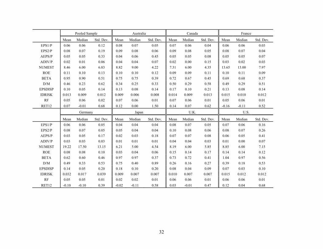
Table 2 reports the descriptive statistics of our variables. The pooled mean of one-year-

ahead (two-year-ahead) analyst earnings forecasts scaled by stock prices is 0.06 (0.08). The

country average two-year-ahead earnings forecasts scaled by stock prices vary from 0.05 (in

Japan) to 0.10 (in the U.K.). This cross-country variation might be due to the definitional

difference of earnings or the differences of expected earnings growth and risks across countries.

The cross-country variation of the actual earnings scaled by stock prices can be explained by

similar reasoning. The mean of the dividend yield varies from 0.01 (in Japan and the U.S.) to

0.04 (in Australia and the U.K.). This cross-country variation might be due to the difference of

dividend payout tendency and tax treatment of dividends across countries.

On the other hand, the cross-country variations of the mean return on equity (from 0.03 of

Japan to 0.15 of the U.K.), of the mean risk-free rate (from 0.02 of Japan to 0.07 of Austria and

Canada) and of the mean stock returns (from -0.16 of France to 0.14 of Canada) reflect the

varying economic conditions across countries. The cross-country variation in risk proxies

indicates the differences of the ex ante firm characteristics related to risk factors across countries.

Note that the average beta is below one for some countries. This might reflect a potential

selection bias within our sample toward the firms with lower systematic risks. Since the pooled

median analyst followings is six, using consensus of analyst earnings forecasts may cancel out 12 As noted by Gode and Mohanram (2003), empirical implementation of the OJ model requires this condition.

16

extreme errors in individual analysts’ earnings forecasts. In sum, the descriptive statistics of

main variables indicate variation in economic conditions as well as of the accounting standards

across countries. Such cross-country variation will tend to increase the power of our test.

Table 3 presents the descriptive statistics of the risk premium estimates for each country.

Investigating the aggregate market level cost of equity, Claus and Thomas (2001) conclude that

the average implied risk premium derived from the RIV model is around 3% in six developed

countries, below the historically average ex post risk premium of 7% to 9%. Consistent with

their findings, our implied risk premium derived from the RIVC model is slightly below 3%.

Although the RIVI model yields higher implied risk premium than the RIVC model, the level of

implied risk premium remains below the historical average ex post risk premium. However, the

OJ model and the PEG model produce consistently higher implied risk premium than the RIV

model. This result might arise from more optimistic assumptions about future earnings growth

by the OJ and PEG models.

Further note that the ex post returns remain more volatile than the implied risk premium:

The standard deviation of the ex post returns (RET12) is lowest for Germany at 38.5%, whereas

the standard deviations of our implied costs of equity always remain below 8%. This supports

the observation in Fama and French (1997), among others, that estimating the cost of equity

based on ex post cost of equity introduces additional noise.

4.3 Descriptive Statistics of the Violations of Clean Surplus

This section reports descriptive evidence on the cross-country variation in the extent to

which the clean surplus relation (hereafter CSR) holds. As noted before, the CSR violation

might affect the validity of the RIV model, but not of the OJ model, and so the cross-country

17

variation in the extent of the CSR violation might lead to the differential relative reliability of the

implied cost of equity derived from the RIV model or the OJ model across countries.

As noted by Frankel and Lee (1999), accounting standards often allow select (value-

relevant) accounting items to be charged directly to the book value of equity without going

through the income statement. These ‘dirty surplus adjustments’ violate the CSR. For example,

under the U.S. GAAP, unrealised gains and losses on marketable securities, foreign currency

translation gains and losses, and gains and losses on derivative instrument, among others, are

charged directly to the book value of equity not through the income statement. Similarly, in

countries such as the U.K., Australia and France, fixed assets may be revealed to reflect their

market value, with a corresponding adjustment directly to the book value of equity. Another

example is the goodwill written off directly against the book value of equity under the U.K.

GAAP during the first half of our sample period. Occasionally, this direct write-off is used by

German firms. In countries such as France and Australia, foreign currency translation tends to

be an important source of the dirty surplus adjustments.

In local GAAP, the existence of the dirty surplus adjustments does not necessarily lead to

the noise in the intrinsic value estimates based on the RIV model. As indicated by Claus and

Thomas (2001), if future earnings expectations, proxied by analyst earnings forecasts in our

study, satisfy the CSR, the validity of the RIV model should remain unaffected. The effect of

analyst forecasts’ violation of the CSR on the validity of the RIV model implementation can be

described as follows. Based on the assumption of the CSR, we start from the prior year’s actual

book value of equity, and add earnings forecast, then subtract forecasted dividend. This gives us

a predicted book value of equity. If analysts’ expectations on the future book value of equity

deviate from the predicted book value of equity, our intrinsic value estimates might differ from

18

the firm values in analysts’ minds. This difference will also bias the implied cost of equity,

which is derived from the assumed equation between stock prices and analysts’ valuations.

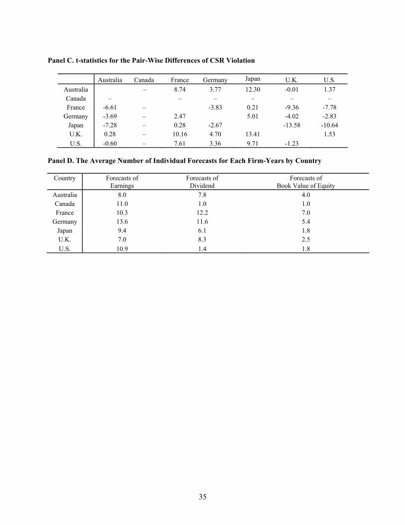
We provide the descriptive evidence of ex ante violation of the CSR from three sets of

consensus analyst forecasts from I/B/E/S. Specifically we require that three sets of consensus

forecasts on book value of equity, earnings, and dividends are available for each firm-year.

Panel A and B of Table 4 show that analyst forecasts do not satisfy the CSR in the ex ante sense

and the extent of the CSR violation varies across countries. Panel C further demonstrates that

this cross-country variation is statistically significant. However, the extent of the ex ante CSR

violation is also affected by the inconsistency of the individual forecast pools, which are used to

calculate the consensus forecasts. As shown in Panel D, such inconsistency varies across

countries. For example, the consensus earnings forecast for a typical U.S. firm-year comes from

about 11 individual forecasts, while the other consensus forecasts are calculated from about 2

individual forecasts. However, in France, each of consensus forecasts appears to be based on

more consistent pool of individual forecasts. In addition, as shown in Panel A, the available

sample is small for Canada, among others. Thus we cannot reliably compare the extent of the ex

ante CSR violation across countries.

Given this limitation in data, we report the ex post violation of the CSR as another

descriptive evidence. Our implicit assumption is that analyst earnings forecasts’ potential

violation of the CSR may be proportional to the magnitude of the ex post violation of the CSR in

our sample. Under this assumption, the effect of the potential CSR violation of analyst earnings

forecasts on the validity of the RIV model can be tested indirectly by examining whether the

cross-country variation of the relative reliability of the implied cost of equity derived from the

RIV model or the OJ model has a relationship with this ex post violation of the CSR.

19

We measure the magnitude of the ex post CSR violation by the difference between the

comprehensive income13 and the net income14 scaled by the book value of equity (hereafter

DSPB), following Lo and Lys (2001). To describe the general magnitude of the CSR violation

within a country, we include all of the firm-years for which the required data for the CSR

analysis are available. Figure 1 represents for each country the cumulative distributions of

DSPB with the familiar S-shape arising from a bell-curved histogram. The U.K. clearly appears

to be second order stochastically dominated by U.S., Japan, Australia and Canada, but

comparable to France and Germany. Recall that second order stochastic dominance implies that

CSR deviations contain additional noise in the European countries. It is therefore not surprising

when we also find that the variance of deviations from CSR is higher among the European

countries.

Panel A of Table 5 reports the distribution of the DSPB within each of the seven countries.

The interquartile range of the DSPB distributes from 1% (Australia) to 6% (France).15 This

measure implies roughly that for half of the firms, the CSR violations of Australian firm-years

exceed 0.05% of the book value of equity while half of French CSR violations exceed 3%. Panel

13 In Global Vantage (abbreviated GV), retained earnings do not include all dirty surplus items. We therefore measure the comprehensive income by the annual change of the sum of a firm’s retained earnings (Global Vantage GV #131), revaluation reserve (GV #130), unappropriated net profit (GV #132), other equity reserves (GV #133), cumulative translation adjustment (GV #134), legal reserves (GV #141) and consolidation reserves (GV #144) adding in common dividends (GV #36). For U.S. firms, however, we follow Dhaliwal, Subramanyam, and Trevazant (1999) and measure the comprehensive income by the annual change in a firm’s retained earnings (Compustat item #36), which includes the dirty surplus items, and add common dividends (Compustat item #21). 14 Global Vantage item #32, except Compustat item #172 for the U.S. firms. 15 We calculate the interquartile range of DSPB as the main metric to assess the magnitude of the CSR violation since the DSPB cannot perfectly measure the CSR violation of the firm-years in the tail. For example, a merging firm’s retained earnings will increase by the merged firm’s retained earnings under the pooling of interest method. Although this is not the violation of the CSR, our DSPB measure will account this increase as the violation of the CSR. It is conceivable that the firm-years in the tail will be affected by these non-dirty surplus items to a relatively larger extent. However, the interquartile range can mitigate this concern since the statistic is not affected by the firm-years in the tail. In addition, this statistic is sensible only when the middle of the distribution is zero. As indicated by Panel A of Table 5, the median of the distribution is around zero within all countries.

20

C of Table 5 reports the t-statistics based on bootstrap-type analysis, 16 indicating that the

differences of interquartile ranges across countries are statistically significant in most cases. As

a supplementary metric, Panel B of Table 5 reports the mean of the absolute DSPB and the

percentage of sample whose absolute DSPB is below 3% or 10%.17 The mean of the absolute

DSPB distributes from 5% (Australia) to 13% (the U.K.). Panel C of Table 5 indicates that the

cross-country differences on the mean of the absolute DSPB are statistically significant.

Moreover, Panel B of Table 5 shows that 43% (78%) of French (Japanese) firm-years has the ex

post CSR violation smaller than 3% of the book value of equity. Bootstrap t-statistics

(untabulated) indicate that the cross-country differences of the percentage with absolute DSPB is

below 3% or 10% are statistically significant.

Although we measure the magnitude of the CSR violation in several different ways, all

measures uniformly indicate that there are significant ex post violations of the CSR within all of

the countries. Further, the cross-country differences of the magnitude of the CSR violation are

significant. On the basis of these measures, we classify Australia, Canada, Japan, and the U.S. as

the countries where the CSR violation is relatively small and classify France, Germany and the

U.K. as the countries where the CSR violation is relatively large.

In sum, we observe a significant violation of the ex post CSR within all of our countries,

and the cross-country variation of the ex post CSR violation is significant. Assuming that the ex

post CSR violation is positively related to the ex ante CSR violation, the cross-country variation

of the CSR violation will set a good empirical setting in which we can examine the effects of the

16 The bootstrap-type analysis results in 95,485 firm-years by drawing observations randomly from the constructed sample with replacement. For each trial, we compute the interquartile range of the DSPB for each country and then compute the difference of interquartile range across countries. This process is repeated 100 times and a distribution for the difference of interquartile range across countries is obtained. A t-statistic is computed as the mean divided by the standard deviation of this distribution. 17 Unlike the interquartile range, this measure is unaffected by cross-country variation in skewness and by the firm-years in the tails.

21

CSR violation on the validity of the RIV model. However, as we pointed out, our ex post CSR

violation is an imperfect measure for the ex ante CSR violation. Therefore, we consider the

analysis concerning the ex post CSR violation only as preliminary, descriptive evidence.

5. Empirical Results

5.1 Univariate Analysis

In this section, we report the pair-wise correlations of key variables. Panel A of Table 6

presents Pearson correlations between implied costs of equity. First, as expected, the implied

costs of equity derived from the OJ model are very highly correlated with the implied costs of

equity derived from the PEG model within all of the countries. Second, the implied costs of

equity derived from the RIVC and RIVI model are more highly correlated with each other than

with costs of equity derived from the OJ or PEG model within all of the countries. That the

correlations among the implied costs of equity emerging from different valuation models remain

below one unit supports that the implied costs of equity exhibit different degrees of reliability.

Panel B of Table 6 reports the Pearson correlations between the risk proxies. Many of these

correlations are significantly different from zero. This suggests that multicollinearity may

prevent the detection of statistical significance of the coefficients on risk proxies. Panel C of

Table 6 presents the Pearson correlation between our risk proxies and the implied costs of equity.

Within all countries, the implied costs of equity are significantly correlated with the risk proxies

in a manner consistent with our expectations. The correlations between the implied costs of

equity and realised stock returns are often insignificant, or even negative, within five out of

seven countries with Japan and the U.S. as notable exceptions. Overall, the implied cost of

equity appears to be a reasonable proxy for the ex ante cost of equity in all of the countries, and

22

the ex ante cost of equity inferred from the implied cost of equity can differ significantly from

the ex ante cost of equity proxied by the realised stock returns.

Since most of the implied costs of equity are significantly correlated with most of risk

proxies, it is difficult to evaluate the relative reliability of the implied costs of equity exclusively

on the basis of univariate correlations. Therefore, we report multivariate regressions which

compare the overall associations between the implied costs of equity and the risk proxies.

5.2 Multivariate Analysis

This section discusses the results of our multivariate regression tests. We regress the

alternative implied costs of equity on the individual risk proxies as the independent variables.18

We then assess which valuation model produces more reliable implied cost of equity by

identifying the implied cost of equity that produces a higher adjusted 2R within each country.

Since the coefficients of risk proxies can be biased due to the multicollinearity problem, we

discuss only the salient features of the coefficients of the risk proxies in following analysis.19

Specifically, to remove the effects of cross-sectional correlation in error terms inherent in

panel data and to allow the coefficient of risk proxies to change in each year, we follow the Fama

and MacBeth (1973) approach to regression analyses. This procedure involves two steps. First,

we estimate the regression model separately for each year of data in the sample. Next, the

coefficients and adjusted 2R from each of these regressions are averaged across all years. We

report the means of the estimated coefficients and the adjusted 2R along with t-statistics based

18 To control the effect of the risk-free rate, we use the implied risk premium as the dependent variable. 19 As an example, for Australia, the pair-wise correlation analysis (in Panel C of Table 6) indicates that all of the implied costs of equity have significant correlations with four out of five risk proxies. However, Panel A of Table 7 indicates that a single risk proxy impacts all of the implied costs of equity.

23

on the time-series standard errors of the individual estimated coefficients with correction for

serial correlation.20

Panel A of Table 7 reports the results of this regression. Consider the polar cases of

Australia and France. In Australia, the RIVI model produces the highest adjusted 2R of 0.47.

The RIVC model produces a relatively high adjusted 2R of 0.35. In contrast, the OJ (PEG)

model generates low adjusted 2R of 0.16 (0.18). Consider next the pattern observed for France:

The OJ and PEG models result in high 2R s of 0.43 while the RIVC (RIVI) model generates

lower 2R of 0.32 (0.30). As indicated in Panel B of Table 7, the differences between the two

RIV-based models and the two OJ-based models are statistically significant but ordered

reversely.21 Canada, Japan, and U.S. offer evidence similar to Australia. This is as we would

expect since the ex ante deviations from the clean surplus relation are lowest in these countries.

While for Germany and the U.K., the differences between valuation models based on RIV and

OJ are statistically insignificantly, the results are qualitatively more similar to France than

Australia. Again, this evidence is consistent with our argument that the OJ and PEG models

should perform relatively better in countries with large ex ante deviations from clean surplus,

which we documented in Section 4.3.

As a supplementary test, not reported, we include the logarithm of the book-to-market ratio

in our regression in table 7. Prior studies view the book-to-market ratio as a proxy for risk

(Griffin and Lemmon, 2002, and Berk, 1995) or mispricing (Daniel and Titman, 1997). If the

book-to-market ratio reflects mispricing of stocks rather than risks, as suggested by several 20 Following Bernard (1995), we adjust the t-statistics for serial correlation, assuming the annual coefficients follow

a first-order autoregressive process. The correction factor is 2[(1 ) /(1 )] [2 (1 ) / (1 )n nφ φ φ φ φ+ + − − − ] where φ is the serial correlation in the coefficient and n is the number of years. 21 This bootstrap-type analysis results in 31,199 firm-years. For each trial, we compute the adjusted R from four valuation models within each country and then compute the difference of adjusted across four valuation models. Proceeding as described in footnote 15, we generate t-statistics.

2

2R

24

studies, our analysis based on adjusted 2R would be mechanically biased toward a more

favorable evaluation of the RIV model. In addition, the book-to-market ratio being used to

impute the RIV-based costs of equity could mechanically affect its association with the implied

costs of equity and generate higher adjusted 2R s. Our untabulated results confirm this, but the

relative orderings remain qualitatively robust.

In summary, the RIV model clearly outperforms the OJ model (including the PEG model)

within all non-European countries that we consider in terms of the adjusted 2R . Furthermore,

despite its theoretical foundation, the OJ model appears to offer little advantage at the

implementation stage in compared to the PEG model, a naïve heuristic for valuation. In addition,

the violation of the CSR seems to affect the relative performance of the RIV and OJ models.

6. Conclusion

We examine the relative reliability of the implied costs of equity within seven developed

countries. We conclude that the implied costs of equity derived from the RIV models are more

reliable than those implied from the OJ model in non-European countries. In Europe the OJ

model performs better – or as well as – the RIV model. Further, we document that the ex ante

violation of the clean surplus relation within a country affects which accounting-based valuation

model produces the more reliable implied costs of equity.

Our analyses and findings invariably suffer from limitations. First, we examine

representative implementations of valuation models, applied by prior research. Heterogeneity in

analysts’ information processing and valuation heuristics, may induce measurement error in the

relative reliability of implied cost of equity. To investigate this, future research might

incorporate other, industry-specific information into the valuation models. Second, our approach

25

uses the association between the implied cost of equity and risk proxies as the metric for the

reliability of the implied cost of equity. An implicit assumption is that considered risk proxies

represent the full list of the ‘true’ risk factors. Omitted, correlated risk proxies may affect our

results. Third, we consider only seven developed countries. Therefore, our findings need not

generalise to a larger cross-section of countries. Despite these caveats, we believe that our

findings offer insights into the derivation of the implied cost of equity closer to the true,

unobservable expected cost of equity.

References

Ali, A., Hwang, L., and Trombley, M. (2003). ‘Residual-income-based valuation predicts future stock returns: Evidence on mispricing vs. risk explanations’. Accounting Review, 78 (April): 377-396. Amihud, Y., and Mendelson, H. (1986). ‘Asset pricing and the bid-ask spread’. Journal of Financial Economics, 17 (2): 223-249. Berk, J. (1995). ‘A critique of size related anomalies’. Review of Financial Studies, 8: 275-286. Bernard, V. (1995). ‘The Feltham-Ohlson framework: Implications for empiricists’. Contemporary Accounting Research, 11 (2): 733-747. Botosan, C. A., and Plumlee, M. A. (2002). ‘Assessing alternative proxies for the expected risk premium’. Working paper, University of Utah. Bradshaw, M. T. (2002). ‘The use of target prices to justify sell-side analysts’ stock recommendations’. Accounting Horizons, 16 (March): 27-41. Bradshaw, M. T. (2004). ‘How do analysts use their earnings forecasts in generating stock recommendations?’ Accounting Review, 79 (January). Claus, J., and Thomas, J. (2001). ‘Equity premia as low as three percent? Evidence from analysts’ earnings forecast for domestic and international stock market’. Journal of Finance, 56 (5): 1629-1666. Daniel, K., and Titman, D. (1997). ‘Evidence on the characteristics of cross-sectional variation in stock returns’. Journal of Finance, 52: 1-33.

26

Dhaliwal, D., Subramanyam, K.R., and Trevazant, R. (1999). ‘Is comprehensive income superior to net income as a measure of firm performance?’ Journal of Accounting and Economics, 26: 43-67. Easton, P. (2004). ‘PE ratios, PEG ratios, and estimating the implied expected rate of return on equity capital’. Accounting Review, 79 (January). Easton, P., and Monahan, S. (2003). ‘An evaluation of the reliability of accounting based measures of expected returns: A measurement error perspective’. Working paper, University of Notre Dame. Elton, E. J. (1999). ‘Expected return, realized return, and asset pricing tests’. Journal of Finance, 54 (4): 1199-1220. Fama, E. F., and French, K. R. (1997). ‘Industry cost of equity’. Journal of Financial Economics, 43: 153-193. Fama, E. F., and MacBeth, J. (1973). ‘Risk, return, and equilibrium: Empirical tests’. Journal of Political Economy, 71: 607-636. Frankel, R. M. (2000). ‘Accounting cross-country accounting differences and fundamental analysis’. Working paper, University of Michigan. Frankel, R., and Lee, C. M. C. (1998). ‘Accounting valuation, market expectation, and cross-sectional stock returns.’ Journal of Accounting and Economics, 25 (June): 283-319. Frankel, R. M., and Lee, C. M. C. (1999). ‘Accounting diversity and international valuation’. Working paper, MIT and Cornell University. Gebhardt, W., Lee, C. M. C., and Swaminathan, B. (2001). ‘Toward an implied cost of capital’. Journal of Accounting Research, 39 (1): 135-176. Gode, D. K. K., and Mohanram, P. (2003). ‘Inferring the cost of capital using the Ohlson-Juettner model’. Review of Accounting Studies, forthcoming. Griffin, J. M., and Lemmon, M. L. (2002). ‘Book-to-market equity, distress risk, and stock returns’. Journal of Finance, 57 (5): 2317-2336. Guay, W., Kothari, S. P., and Shu, S. (2003). ‘An empirical assessment of cost of capital measures’. Working paper, MIT. Lee, C. M. C., Myers, J., and Swaminathan, B. (1999). ‘What is the intrinsic value of the Dow?’ Journal of Finance, 54: 1693-1741. Lehmann, B. N. (1990). ‘Residual risk revisited’. Journal of Econometrics, 45: 71-97.

27

Liu, J., Nissim, D., and Thomas, J. (2002). ‘Valuation using multiples’. Journal of Accounting Research, 40 (1): 135-172. Lo, K., and Lys, T. (2001). ‘The Ohlson model: Contribution to valuation theory, limitations, and empirical applications’. Journal of Accounting, Auditing, and Finance, 15 (3): 337-367. Malkiel, B. G., and Xu, Y. (1997). ‘Risk and return revisited’. Journal of Portfolio Management, 23: 9-14. Modigliani, F., and Miller, M.H. (1958). ‘The cost of capital, corporation finance and the theory of investment’. American Economic Review, 48 (3): 261-297. Myers, J. N. (1999). ‘Implementing residual income valuation with linear information dynamics’. Accounting Review, 74 (January): 1-28. Ohlson, J. A., (1995). ‘Earnings, book values, and dividends in security valuation’. Contemporary Accounting Research, 11 (Spring): 661-687. Ohlson, J. A., and Juettner-Nauroth, B. E. (2000). ‘Expected EPS and EPS growth as determinants of value’. Working paper, New York University. Penman, S. H. (2004). Financial Statement Analysis and Security Valuation. 2nd edition, New York, NY: McGraw-Hill. Ross, S. A. (1976). ‘The arbitrage theory of capital asset pricing model (CAPM)’. Journal of Economic Theory, 13: 341-360. Walker, M. (1997). ‘Clean surplus accounting models and market-based accounting research: A review’. Accounting and Business Research, 27 (4): 341-355. Appendix In this appendix we prove, as claimed in footnote 2, that ex post clean surplus violations should not affect the infinite horizon empirical implementation of the RIV model. Denote the most recently observed historical book value by bv and analyst earnings forecasts by

. The book value includes retained earnings which are the accumulation of earnings (or comprehensive income) from all prior years less the accumulated dividends. Consider what would happen if analysts, for the purpose of forecasting future earnings, apply a different definition or standard of earnings than that applied by the firm in prior years. Let bv denote the accounting book value that would have been reported in the initial year t if the firm had applied the analysts’ definition of earnings. This creates an initial discrepancy,

, in the application by empirical researchers of historical book value, bv , and analyst earnings forecasts. Since empirically, future book values are created by rolling forward

t

1 2, ,...,t teps eps eps+ +

at tbv bv bv∆ = −

5t+

at

t

28

through the clean surplus relation, all future book values will be misstated by the exact same amount, that is, ∆ = . However, this potential measurement error rinses out in the valuation of the firm since:

at n t nbv bv bv+ −

( )( ) ( )

( )

( )( )

1 2

1 2

1

t t t

t t

t t t

bv eps r

eps r bv

r

r bv eps

r r

+ +

+ +

− ⋅ − ⋅+ +

− ++

+

− ⋅+

+

( ) ( )( )

( ) ( )( ) ( )( )( )

( )( )( )

( )( )

( )

1 3 22 3

1 2 1 3 2

2 3

1 3 22

...1 1 1

...1 1

1 1 1

t t tt

a a at t t ta

t

a a at t ta

t

eps r bv eps r bvbv

r r r

bv eps r bv bv eps r bv bvbv bv

r r

eps r bv eps r bvbv

+ + +

+ + + + +

+ + +

− ⋅+ +

+ + +

∆ − + ∆ − + ∆= + ∆ + + +

+ +

− ⋅ − ⋅= + +

+ + +( )3 ...r

+

where the last equality follows from the identity that ( ) ( ) ( )2 3 ...1 1 1

bv bv bvbv r

r r r

∆ ∆ ∆= ∆ −

+ + +0

+ + +

.

This completes our proof. Note that this does not rule out that ex ante clean surplus violations may affect the empirical implementation of the RIV model.

29

Table 1. Descriptive Statistics for Sample Countries

Panel A. Firms per Year by Country

Year Australia Canada France Germany Japan U.K. U.S. 1993 80 127 28 37 407 396 1,672 1994 100 167 101 107 454 411 1,785 1995 111 180 117 102 828 467 1,942 1996 119 187 149 112 993 545 2,071 1997 154 178 176 126 850 563 2,079 1998 155 167 2 0 762 546 2,111 1999 140 157 25 2 761 509 1,981 2000 135 121 64 34 730 211 1,640 2001 118 109 98 74 758 246 1,622

Total Firm-Years 1,112 1,393 760 594 6,543 3,894 16,903 Number of Firms 221 314 243 195 1,490 850 3,979

Panel B. Observations per Sector by Country (in %)

Sector Australia Canada France Germany Japan U.K. U.S. Health Care 3% 2% 6% 6% 4% 4% 11%

Consumer Non-Durables 10 6 13 11 12 13 7 Consumer Services 24 21 27 17 19 28 20 Consumer Durables 3 3 3 5 6 3 6

Energy 8 23 3 0 1 2 7 Transportation 2 2 3 1 4 3 3

Technology 2 5 3 3 10 8 18 Basic Industries 32 22 11 18 13 12 9 Capital Goods 14 10 30 33 28 27 11 Public Utilities 1 7 1 6 2 2 8

Total 100% 100% 100% 100% 100% 100% 100%

30

Table 2. Descriptive Statistics of Variables for the Pooled Sample and by Country This table presents the mean, median and the standard deviation of variables used in this paper for the pooled sample and by country. EPS1/P is the one-year-ahead consensus analyst earnings forecast scaled by stock price. EPS2/P is two-year-ahead consensus analyst earning forecast scaled by stock price. AEPS/P is the actual earnings per share scaled by stock price. ADIV/P is the actual dividend per share scaled by stock price. NUMEST is the number of earnings forecasts. All forecasts are from the September statistical period from I/B/E/S. ROE is the return on book value of equity. BETA is the systematic risk estimated by regressing at least 30 prior monthly returns up to 60 prior monthly returns against the corresponding market index in each country. EPSDISP is the dispersion of analyst earnings forecasts, which is measured as the standard deviation of the one-year-ahead earnings forecasts scaled by the absolute mean of these forecasts. IDRISK is the idiosyncratic risk, which is measured as the variance of residuals from the regressions of beta estimation. RF is the risk-free rate, as proxied by the 10-year long-term government bond rate in each country. RET12 is the realised annual stock return.

31

Pooled Sample Australia Canada France

Mean Median Std. Dev. Mean Median Std. Dev. Mean Median Std. Dev. Mean Median Std. Dev. EPS1/P 0.06 0.06 0.12 0.08 0.07 0.05 0.07 0.06 0.04 0.06 0.06 0.03EPS2/P 0.08 0.07 0.19 0.09 0.08 0.06 0.09 0.08 0.05 0.08 0.07 0.04AEPS/P 0.05 0.05 0.33 0.04 0.06 0.45 0.05 0.05 0.08 0.05 0.05 0.07ADIV/P 0.02 0.01 0.06 0.04 0.04 0.07 0.02 0.00 0.15 0.03 0.02 0.03

NUMEST 8.46 6.00 6.83 8.82 9.00 4.22 7.31 6.00 4.35 13.65 13.00 7.97ROE 0.11 0.10 0.13 0.10 0.10 0.12 0.09 0.09 0.11 0.10 0.11 0.09

BETA 0.95 0.90 0.51 0.75 0.75 0.39 0.72 0.67 0.45 0.69 0.68 0.37D/M 0.46 0.23 0.62 0.34 0.25 0.33 0.50 0.29 0.58 0.49 0.29 0.51

EPSDISP 0.10 0.05 0.14 0.13 0.08 0.14 0.17 0.10 0.21 0.13 0.08 0.14IDRISK 0.013 0.009 0.012 0.009 0.006 0.008 0.014 0.009 0.013 0.015 0.010 0.012

RF 0.05 0.06 0.02 0.07 0.06 0.01 0.07 0.06 0.01 0.05 0.06 0.01RET12 0.07 -0.01 0.68 0.12 0.00 1.50 0.14 0.07 0.62 -0.16 -0.11 0.52

Germany Japan U.K. U.S.

Mean Median Std. Dev. Mean Median Std. Dev. Mean Median Std. Dev. Mean Median Std. Dev. EPS1/P 0.06 0.06 0.05 0.04 0.04 0.04 0.08 0.07 0.05 0.07 0.06 0.16EPS2/P 0.08 0.07 0.05 0.05 0.04 0.04 0.10 0.08 0.06 0.08 0.07 0.26AEPS/P 0.03 0.05 0.17 0.02 0.03 0.18 0.07 0.07 0.08 0.06 0.05 0.41ADIV/P 0.03 0.03 0.03 0.01 0.01 0.01 0.04 0.04 0.03 0.01 0.00 0.07

NUMEST 19.22 17.50 13.15 6.21 5.00 4.54 8.19 6.00 5.85 8.85 6.00 7.15ROE 0.08 0.08 0.10 0.03 0.04 0.06 0.15 0.14 0.17 0.14 0.14 0.12

BETA 0.62 0.60 0.46 0.97 0.97 0.37 0.73 0.72 0.41 1.04 0.97 0.56D/M 0.49 0.33 0.53 0.75 0.40 0.89 0.26 0.16 0.27 0.39 0.18 0.53

EPSDISP 0.14 0.05 0.20 0.18 0.10 0.20 0.08 0.04 0.09 0.07 0.03 0.10IDRISK 0.032 0.017 0.039 0.009 0.007 0.007 0.010 0.007 0.007 0.015 0.012 0.012

RF 0.05 0.05 0.01 0.02 0.02 0.01 0.06 0.06 0.01 0.06 0.06 0.01RET12 -0.10 -0.10 0.39 -0.02 -0.11 0.58 0.03 -0.01 0.47 0.12 0.04 0.68

32

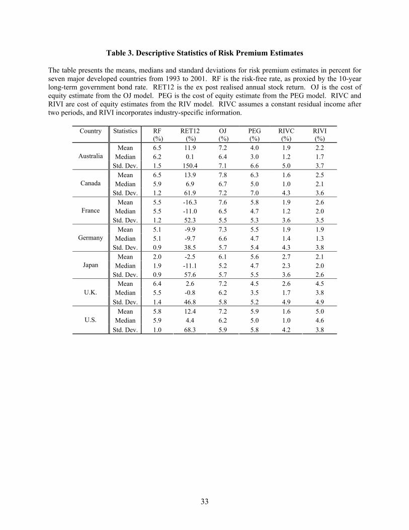
Table 3. Descriptive Statistics of Risk Premium Estimates The table presents the means, medians and standard deviations for risk premium estimates in percent for seven major developed countries from 1993 to 2001. RF is the risk-free rate, as proxied by the 10-year long-term government bond rate. RET12 is the ex post realised annual stock return. OJ is the cost of equity estimate from the OJ model. PEG is the cost of equity estimate from the PEG model. RIVC and RIVI are cost of equity estimates from the RIV model. RIVC assumes a constant residual income after two periods, and RIVI incorporates industry-specific information.

Country

Statistics

RF (%)

RET12 (%)

OJ (%)

PEG (%)

RIVC (%)

RIVI (%)

Mean 6.5 11.9 7.2 4.0 1.9 2.2 Median 6.2 0.1 6.4 3.0 1.2 1.7 Australia

Std. Dev. 1.5 150.4 7.1 6.6 5.0 3.7 Mean 6.5 13.9 7.8 6.3 1.6 2.5

Median 5.9 6.9 6.7 5.0 1.0 2.1 Canada Std. Dev. 1.2 61.9 7.2 7.0 4.3 3.6

Mean 5.5 -16.3 7.6 5.8 1.9 2.6 Median 5.5 -11.0 6.5 4.7 1.2 2.0 France

Std. Dev. 1.2 52.3 5.5 5.3 3.6 3.5 Mean 5.1 -9.9 7.3 5.5 1.9 1.9

Median 5.1 -9.7 6.6 4.7 1.4 1.3 Germany Std. Dev. 0.9 38.5 5.7 5.4 4.3 3.8

Mean 2.0 -2.5 6.1 5.6 2.7 2.1 Median 1.9 -11.1 5.2 4.7 2.3 2.0 Japan

Std. Dev. 0.9 57.6 5.7 5.5 3.6 2.6 Mean 6.4 2.6 7.2 4.5 2.6 4.5

Median 5.5 -0.8 6.2 3.5 1.7 3.8 U.K. Std. Dev. 1.4 46.8 5.8 5.2 4.9 4.9

Mean 5.8 12.4 7.2 5.9 1.6 5.0 Median 5.9 4.4 6.2 5.0 1.0 4.6 U.S.

Std. Dev. 1.0 68.3 5.9 5.8 4.2 3.8

33

Table 4. Ex Ante Violation of the Clean Surplus Relation This table presents the descriptive statistics of ex ante violation of the clean surplus relation for each sample country. The ex ante CSR violation is calculated as the difference between the book value of equity forecasted by the analysts and the book value predicted from the prior year actual book value, adding analyst earnings forecast, and subtracting analyst dividend forecasts, which is then scaled by the prior year actual book value of equity. Panel A presents the mean, median, the standard deviation, and the interquartile range. We winsorise the ex ante CSR violation at -1 and 1. Panel B presents ex ante CSR violations in absolute values, which are winsorised at 1. Similar statistics are presented in Panel B. In addition, ADS3% (ADS10%) is the percentage of firm-years with CSR violation smaller than 3% (10%) of prior year actual book value of equity. Panel C presents the t-statistics for the difference of CSR violation. The upper triangle reports t-statistics for the differences of mean absolute CSR violation presented in Panel B. The lower triangle reports the bootstrap t-statistics for the differences of interquartile range statistics presented in Panel A. The critical value for the pair-wise t-test is 1.96. Panel D presents the average number of individual earnings, dividend and book value of equity forecasts consisting of the consensus forecasts in each country. Panel A. The Distribution of Ex Ante CSR Violation per Book Value of Equity

Country No. of

firm-years Mean Median Std. Dev. Interquartile

Range Australia 1,081 -0.13 -0.05 0.37 0.24 Canada 1 0.40 0.40 – – France 640 -0.08 -0.01 0.23 0.11

Germany 411 0.00 0.00 0.31 0.16 Japan 1,447 -0.06 -0.04 0.22 0.11 U.K. 2,026 -0.13 -0.04 0.36 0.25 U.S. 838 -0.02 0.02 0.35 0.23

Panel B. The Distribution of Ex Ante CSR Violation in Absolute Values per Book Value of Equity

Country Mean Median Std. Dev. ADS3% ADS10% Australia 0.24 0.11 0.30 0.20 0.47 Canada 0.40 0.40 - – – France 0.13 0.05 0.21 0.36 0.71

Germany 0.18 0.07 0.25 0.30 0.58 Japan 0.13 0.06 0.19 0.27 0.66 U.K. 0.24 0.12 0.30 0.20 0.45 U.S. 0.23 0.12 0.27 0.18 0.45

34

Panel C. t-statistics for the Pair-Wise Differences of CSR Violation

Australia Canada France Germany Japan U.K. U.S. Australia – 8.74 3.77 12.30 -0.01 1.37 Canada – – – – – – France -6.61 – -3.83 0.21 -9.36 -7.78

Germany -3.69 – 2.47 5.01 -4.02 -2.83 Japan -7.28 – 0.28 -2.67 -13.58 -10.64 U.K. 0.28 – 10.16 4.70 13.41 1.53 U.S. -0.60 – 7.61 3.36 9.71 -1.23

Panel D. The Average Number of Individual Forecasts for Each Firm-Years by Country

Country

Forecasts of Earnings

Forecasts of Dividend

Forecasts of Book Value of Equity

Australia 8.0 7.8 4.0 Canada 11.0 1.0 1.0 France 10.3 12.2 7.0

Germany 13.6 11.6 5.4 Japan 9.4 6.1 1.8 U.K. 7.0 8.3 2.5 U.S. 10.9 1.4 1.8

35

Table 5. Ex Post Violation of the Clean Surplus Relation

This table presents the descriptive statistics of ex post violation of the clean surplus relation for each sample country. The ex post CSR violation is calculated by the difference between the comprehensive income and the net income scaled by the book value of equity. Panel A presents the mean, median, the standard deviation, and the interquartile range. We winsorise the ex post CSR violation at -1 and 1. Panel B presents the ex post CSR violations in absolute values, which are winsorised at 1. Similar statistics are presented in Panel B. In addition, ADS3% (ADS10%) is the percentage of firm-years with CSR violation smaller than 3% (10%) of book value of equity. Panel C presents the t-statistics for the difference of CSR violation. The upper triangle is t-statistics for the differences of mean absolute CSR violation presented in Panel B. The lower triangle is the bootstrap t-statistics for the differences of interquartile range statistics presented in Panel A. The critical value for the pair-wise t-test is 1.96. Panel A. The Distribution of Ex Post CSR Violation per Book Value of Equity

Country No. of

firm-years Mean Median Std. Dev. Interquartile

Range Australia 2,087 0.011 0.000 0.171 0.009 Canada 3,311 -0.006 0.000 0.208 0.021 France 3,082 -0.027 -0.023 0.205 0.060

Germany 3,264 -0.008 -0.001 0.231 0.056 Japan 16,582 0.007 0.000 0.125 0.013 U.K. 7,425 -0.014 -0.001 0.277 0.054 U.S. 59,734 -0.016 0.000 0.172 0.012

Panel B. The Distribution of Ex Post CSR Violation in Absolute Values per Book Value of Equity

Country Mean Median Std. Dev. ADS3% ADS10% Australia 0.05 0.01 0.16 0.75 0.90 Canada 0.08 0.01 0.19 0.69 0.84 France 0.10 0.04 0.18 0.43 0.78

Germany 0.10 0.03 0.21 0.52 0.78 Japan 0.04 0.01 0.12 0.78 0.93 U.K. 0.13 0.03 0.24 0.52 0.73 U.S. 0.06 0.00 0.16 0.76 0.89

Panel C. t-statistics for the Pair-Wise Differences of CSR Violation

Australia Canada France Germany Japan U.K. U.S. Australia -4.72 -9.35 -9.35 5.34 -13.75 -0.43 Canada 6.47 -4.82 -5.38 15.23 -11.42 7.38 France 25.19 21.38 -0.80 23.65 -6.62 14.48

Germany 16.28 14.14 -1.50 24.56 -5.79 16.05 Japan 3.01 -5.47 -29.19 -17.85 -39.59 -12.52 U.K. 18.55 12.75 -2.65 -0.60 18.44 35.55 U.S. 1.99 -7.02 -31.32 -18.52 -3.66 -19.34

36

Table 6. Correlations of Implied Costs of Equity and Risk Proxies This table presents the Pearson correlations of implied costs of equity and risk proxies for the pooled sample and for each country. OJ is the cost of equity estimate from the OJ model. PEG is the cost of equity estimate from the PEG model. RIVC is the cost of equity estimate from the RIV model assuming a constant residual income after two periods. RIVI is the cost of equity estimate from the RIV model but incorporating industry-specific information. BETA is the systematic risk estimated by regressing at least 30 prior monthly returns up to 60 prior monthly returns against the corresponding market index in each country. MV is the market value of equity for each firm-year. D/M is the debt divided by market value of equity for each firm. EPSDISP is the dispersion of analyst earnings forecasts, which is measured as the standard deviation of the one-year-ahead analyst earnings forecasts scaled by the absolute mean of these forecasts. IDRISK is the idiosyncratic risk, which is measured as the variance of residuals from the regressions of beta estimation. RET12 is the realised annual stock return. ***, **, * indicate, respectively, the significance level at the 1%, 5% and 10% level or better. Panel A. Pearson Correlations Between Implied Costs of Equity

Australia OJ PEG RIVC Canada OJ PEG RIVC PEG 0.97*** PEG 0.99*** RIVC 0.57*** 0.57*** RIVC 0.49*** 0.52*** RIVI 0.47*** 0.48*** 0.79*** RIVI 0.35*** 0.40*** 0.72***

France OJ PEG RIVC Germany OJ PEG RIVC

PEG 0.99*** PEG 0.98*** RIVC 0.54*** 0.55*** RIVC 0.40*** 0.40*** RIVI 0.49*** 0.51*** 0.83*** RIVI 0.31*** 0.30*** 0.59***

Japan OJ PEG RIVC U.K. OJ PEG RIVC PEG 1.00*** PEG 0.97*** RIVC 0.54*** 0.53*** RIVC 0.58*** 0.55*** RIVI 0.42*** 0.40*** 0.72*** RIVI 0.44*** 0.43*** 0.74***

U.S. OJ PEG RIVC Pooled OJ PEG RIVC PEG 0.99*** PEG 0.98*** RIVC 0.48*** 0.51*** RIVC 0.56*** 0.55*** RIVI 0.44*** 0.49*** 0.73*** RIVI 0.51*** 0.51*** 0.71***

37

Panel B. Pearson Correlations Between Risk Proxies and Realised Annual Stock Returns

Australia BETA MV D/M EPSDISP IDRISK Canada BETA MV D/M EPSDISP IDRISKMV 0.12*** MV 0.02 D/M 0.08** -0.02 D/M 0.00 -0.09***

EPSDISP 0.20*** -0.15*** 0.28*** EPSDISP 0.19*** -0.04 0.17***

IDRISK 0.18*** -0.10*** 0.00 0.31*** IDRISK 0.26*** -0.17*** -0.06* 0.17***

Ret12 -0.03 0.00 0.03 -0.02 -0.03 Ret12 -0.08*** -0.05 0.03 0.02 0.05

France BETA MV D/M EPSDISP IDRISK Germany BETA MV D/M EPSDISP IDRISKMV 0.13*** MV 0.23*** D/M 0.01 -0.12*** D/M 0.05 -0.12***

EPSDISP 0.03 -0.14*** 0.37*** EPSDISP 0.06 -0.07* 0.25***

IDRISK -0.03 -0.11*** 0.04 0.06* IDRISK 0.10** -0.04 -0.03 -0.16***

Ret12 -0.04 -0.02 0.09** -0.05 0.07* Ret12 -0.08 0.05 -0.04 -0.15*** 0.15***

Japan BETA MV D/M EPSDISP IDRISK U.K. BETA MV D/M EPSDISP IDRISKMV -0.06*** MV 0.02 D/M 0.08*** -0.04*** D/M 0.02 -0.07***

EPSDISP 0.18*** -0.06*** 0.28*** EPSDISP 0.07*** -0.05*** 0.35***

IDRISK 0.42*** -0.15*** 0.02* 0.12*** IDRISK 0.09*** -0.09*** 0.07*** 0.25***

Ret12 -0.03** -0.01 0.05*** 0.03** 0.02* Ret12 0.04** -0.02 -0.04** -0.04** -0.01

U.S. BETA MV D/M EPSDISP IDRISK Pooled BETA MV D/M EPSDISP IDRISKMV -0.04*** MV -0.03*** D/M -0.17*** -0.07*** D/M -0.06*** -0.02***

EPSDISP 0.09*** -0.07*** 0.24*** EPSDISP 0.07*** 0.02*** 0.31***

IDRISK 0.45*** -0.15*** -0.12*** 0.20*** IDRISK 0.33*** -0.10*** -0.08*** 0.07***

Ret12 0.04*** -0.03*** -0.01 -0.03*** -0.02*** Ret12 0.03*** -0.03*** -0.01 -0.03*** 0.01

38

Panel C. Pearson Correlations Between Implied Costs of Equity and Risk Proxies

Australia OJ PEG RIVC RIVI Canada OJ PEG RIVC RIVI BETA 0.03 0.07** -0.02 0.04 BETA 0.18*** 0.20*** 0.06* 0.10*** MV -0.13*** -0.11*** -0.19*** -0.20*** MV -0.13*** -0.15*** -0.19*** -0.21*** D/M 0.20*** 0.19*** 0.40*** 0.57*** D/M 0.16*** 0.16*** 0.29*** 0.36***

EPSDISP 0.28*** 0.34*** 0.21*** 0.35*** EPSDISP 0.27*** 0.28*** -0.08*** 0.12*** IDRISK 0.10*** 0.20*** 0.17*** 0.21*** IDRISK 0.16*** 0.21*** 0.16*** 0.22*** Ret12 0.01 0.01 0.00 0.01 Ret12 0.04 0.04 0.05 0.08**

France OJ PEG RIVC RIVI Germany OJ PEG RIVC RIVI BETA 0.07* 0.08* -0.05 -0.05 BETA 0.22*** 0.24*** 0.14*** 0.09* MV -0.17*** -0.17*** -0.23*** -0.25*** MV -0.14*** -0.14*** -0.15*** -0.17***

D/M 0.55*** 0.54*** 0.45*** 0.41*** D/M 0.36*** 0.33*** 0.27 0.48*** EPSDISP 0.47*** 0.48*** 0.17*** 0.29*** EPSDISP 0.36*** 0.38*** 0.08* 0.19*** IDRISK 0.14*** 0.14*** 0.15*** 0.25*** IDRISK -0.03 -0.04 -0.05 -0.07* Ret12 0.12*** 0.07* -0.01 -0.07* Ret12 0.04 0.02 0.01 -0.01

Japan OJ PEG RIVC RIVI U.K. OJ PEG RIVC RIVI BETA 0.11*** 0.13*** 0.01 -0.02 BETA 0.05*** 0.04*** -0.07*** -0.09*** MV -0.08*** -0.07*** -0.15*** 0.21*** MV -0.14*** -0.14*** -0.15*** -0.13*** D/M 0.17*** 0.16*** 0.17*** 0.25*** D/M 0.35*** 0.33*** 0.43*** 0.45***

EPSDISP 0.24*** 0.24*** -0.07*** 0.12*** EPSDISP 0.35*** 0.37*** 0.15*** 0.25*** IDRISK 0.33*** 0.35*** 0.37*** 0.29*** IDRISK 0.18*** 0.24*** 0.07*** 0.18*** Ret12 0.12*** 0.12*** 0.21*** 0.23*** Ret12 0.01 0.01 0.05*** 0.05***

U.S. OJ PEG RIVC RIVI Pooled OJ PEG RIVC RIVI

BETA 0.14*** 0.17*** -0.07*** 0.07*** BETA 0.09*** 0.14*** -0.08*** 0.04*** MV -0.13*** -0.15*** -0.14*** -0.20*** MV -0.13*** -0.12*** -0.13*** -0.20*** D/M 0.22*** 0.22*** 0.42*** 0.40*** D/M 0.10*** 0.12*** 0.20*** 0.09***

EPSDISP 0.35*** 0.35*** 0.04*** 0.19*** EPSDISP 0.18*** 0.20*** -0.05*** -0.07*** IDRISK 0.23*** 0.30*** 0.02** 0.223*** IDRISK 0.22*** 0.27*** 0.08*** 0.22*** Ret12 0.03*** 0.03*** 0.04*** 0.03*** Ret12 0.07*** 0.07*** 0.08*** 0.10***

39

Table 7. Cross-Sectional Year-by-Year Regressions of Implied Risk Premia This table presents the cross-sectional year-by-year regressions of implied risk premia for each country. The regression equation is as follows.

RISKPREMIUM (Intercept) BETA MV D/M EPSDISP IDRISKα α α α α ε= + + + + + +1 2 3 4 5it it it it it it it . RISKPREMIUM is defined as the cost of equity estimate minus the country-specific risk free rate. OJ is the cost of equity estimate from the OJ model. PEG is the cost of equity estimate from the PEG model. RIVC is the cost of equity estimate from the RIV model assuming a constant residual income after two periods. RIVI is the cost of equity estimate from the RIV model but incorporating industry-specific information. BETA is the systematic risk estimated by regressing at least 30 prior monthly returns up to 60 prior monthly returns against the corresponding market index in each country. MV is the market value of equity for each firm-year. D/M is the debt divided by market value of equity for each firm. EPSDISP is the dispersion of analyst earnings forecasts, which is measured as the standard deviation of the one-year-ahead earnings forecasts scaled by the absolute mean of these forecasts. IDRISK is the idiosyncratic risk, which is measured as the variance of residuals from the regressions of beta estimation. The coefficients presented are the means from annual regressions. The number below each coefficient is the t-statistic, adjusted for auto-correlation as in Bernard (1995). Adj-R2 is the average adjusted R2 for the regressions. Average sample size is the average number of samples per year for each sample country. Panel B shows the bootstrap t-statistics for the differences of adjusted R2s. The null hypothesis is no difference between any pair of adjusted R2s in the cross-sectional regressions. ***, **, * indicate, respectively, the significance level at the 1%, 5% and 10% level or better. Panel A. Regressions of Implied Risk Premia with Associated Risk Proxies

Country Model Intercept BETA MV D/M EPSDISP IDRISK Adj-R2 No. of Years Average Sample Size

Expected Signs ? + - + + + OJ 0.10 0.12 0.00 -0.01 0.03 -0.31 0.16 9 124

t-stat 12.61 0.32 -15.18 4.23 4.88 -0.53PEG 0.06 0.00 -0.01 0.02 0.11 0.33 0.18 9 124t-stat 6.73 0.55 -12.09 2.48 6.87 0.65RIVC 0.08 0.00 -0.01 0.04 -0.02 -0.02 0.35 9 124t-stat 3.69 0.12 -5.97 2.91 -0.79 -0.04RIVI 0.05 0.00 -0.01 0.04 0.01 0.02 0.47 9 124

Australia

t-stat 2.53 1.17 -5.53 6.21 3.91 0.06OJ 0.09 0.02 -0.01 0.01 0.07 0.31 0.14 9 155

t-stat 2.47 2.82 -1.72 8.94 5.48 0.91PEG 0.08 0.02 -0.01 0.01 0.06 0.44 0.17 9 155t-stat 2.36 2.77 -2.42 7.94 5.18 1.39RIVC 0.05 0.01 -0.01 0.02 -0.04 0.31 0.21 9 155t-stat 2.01 2.07 -3.61 12.45 -4.88 3.32RIVI 0.05 0.01 -0.01 0.02 0.00 0.22 0.30 9 155

Canada

t-stat 1.93 2.41 -4.46 7.79 -0.82 3.98

40

(Panel A continues)

Country Model Intercept BETA MV D/M EPSDISP IDRISK Adj-R2 No. of Years Average Sample Size

Expected Signs ? + - + + + OJ 0.08 0.01 -0.01 0.04 0.11 0.40 0.43 8 95

t-stat 8.06 3.18 -8.00 10.75 11.85 1.03PEG 0.06 0.01 -0.01 0.04 0.10 0.40 0.43 8 95t-stat 7.49 4.27 -10.63 10.48 11.37 1.08RIVC 0.07 0.01 -0.01 0.03 -0.02 -0.28 0.32 8 95t-stat 3.21 0.89 -4.44 3.13 -1.12 -2.13RIVI 0.06 0.01 -0.01 0.02 0.01 -0.11 0.30 8 95

France

t-stat 3.69 0.97 -9.91 4.33 0.49 -0.92 OJ 0.08 0.03 -0.01 0.03 0.06 -0.17 0.25 7 85

t-stat 1.51 4.33 -1.28 8.03 3.25 -2.95PEG 0.05 0.03 0.00 0.02 0.06 -0.13 0.25 7 85t-stat 0.93 4.19 -0.90 4.05 4.21 -2.39RIVC 0.07 0.01 -0.01 0.01 -0.02 -0.24 0.26 7 85t-stat 1.40 5.22 -1.89 5.43 -0.97 -1.11RIVI 0.04 0.01 -0.01 0.02 0.00 -0.13 0.32 7 85

Germany

t-stat 1.25 1.32 -3.80 24.83 -0.88 -1.21OJ 0.09 0.00 0.00 0.00 0.04 0.65 0.11 9 727

t-stat 1.72 1.81 -1.42 1.69 8.73 2.85PEG 0.08 0.00 0.00 0.00 0.04 0.78 0.12 9 727t-stat 1.70 2.23 -1.50 1.50 8.52 3.59RIVC 0.10 0.00 -0.01 0.00 -0.03 0.17 0.29 9 727t-stat 1.66 -1.40 -1.65 0.72 -7.57 1.49RIVI 0.09 0.00 -0.01 0.00 0.00 -0.38 0.33 9 727

Japan

t-stat 1.97 -1.23 -2.24 1.34 0.30 -3.85 OJ 0.15 0.01 -0.01 0.04 0.14 0.37 0.31 9 433

t-stat 4.79 5.61 -5.62 7.35 5.50 3.30PEG 0.11 0.01 -0.01 0.03 0.13 0.73 0.32 9 433t-stat 3.35 4.56 -5.29 7.18 6.15 10.21RIVC 0.11 0.01 -0.01 0.05 -0.02 -0.16 0.30 9 433t-stat 1.87 3.25 -2.56 5.11 -1.73 -0.78RIVI 0.12 0.01 -0.01 0.05 0.02 0.20 0.31 9 433

U.K.

t-stat 1.96 1.48 -2.50 5.73 4.19 1.41

41

(Panel A continues)

Country Model Intercept BETA MV D/M EPSDISP IDRISK Adj-R2 No. of Years Average Sample Size

Expected Signs ? + - + + + OJ 0.09 0.01 -0.01 0.02 0.14 0.41 0.26 9 1,878

t-stat 4.29 9.71 -4.97 4.49 7.49 1.42PEG 0.08 0.01 -0.01 0.01 0.13 0.57 0.30 9 1,878t-stat 3.38 10.08 -5.58 4.61 6.85 1.87RIVC 0.06 0.00 -0.01 0.03 -0.04 -0.21 0.27 9 1,878t-stat 2.63 0.70 -3.25 10.49 -10.11 -1.65RIVI 0.09 0.01 -0.01 0.02 0.00 0.03 0.35 9 1,878

U.S.

t-stat 2.96 6.31 -3.88 12.55 -0.27 0.14 Panel B. t-statistics for the Differences of Adjusted R2

Country OJ PEG RIVC Country OJ PEG RIVC

PEG 2.10** PEG 7.25*** RIVC 5.23*** 4.45*** RIVC 2.69*** 1.60 RIVI 8.52*** 7.64*** 3.77*** RIVI 4.92*** 3.81*** 3.14***

Australia

Canada

PEG 0.69 PEG 0.40 RIVC -1.40 -1.52 RIVC 0.45 0.37 RIVI -1.69* -1.83* -0.42 RIVI 1.32 1.28 1.37

France

Germany

PEG 3.39*** PEG 1.97** RIVC 14.80*** 14.41*** RIVC 0.03 -0.49 RIVI 12.76*** 12.48*** 2.76*** RIVI 0.64 0.16 0.77

Japan

U.K.

PEG 32.38*** RIVC 1.67* -3.01*** RIVI 7.29*** 3.73*** 6.18***

U.S.

42

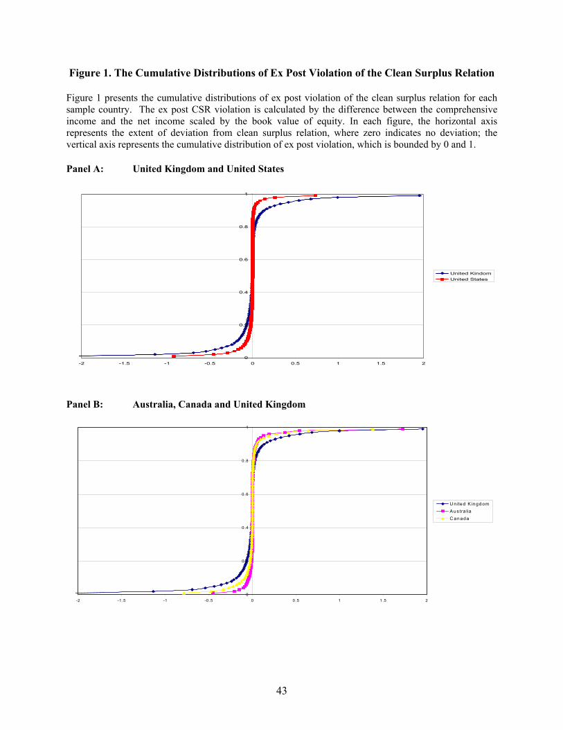
Figure 1. The Cumulative Distributions of Ex Post Violation of the Clean Surplus Relation Figure 1 presents the cumulative distributions of ex post violation of the clean surplus relation for each sample country. The ex post CSR violation is calculated by the difference between the comprehensive income and the net income scaled by the book value of equity. In each figure, the horizontal axis represents the extent of deviation from clean surplus relation, where zero indicates no deviation; the vertical axis represents the cumulative distribution of ex post violation, which is bounded by 0 and 1. Panel A: United Kingdom and United States

0

0.2

0.4

0.6

0.8

1

-2 -1.5 -1 -0.5 0 0.5 1 1.5 2

United KindomUnited States

Panel B: Australia, Canada and United Kingdom

0

0 .2

0 .4

0 .6

0 .8

1

-2 -1 .5 -1 -0 .5 0 0 .5 1 1 .5 2

U n ited K ingd omA us tra liaC an ada

43

Panel C: Japan and United Kingdom

0

0.2

0.4

0.6

0.8

1

-2 -1.5 -1 -0.5 0 0.5 1 1.5 2

United KindomJapan

Panel D: France, Germany, and United Kingdom

0

0.2

0.4

0.6

0.8

1

-2 -1.5 -1 -0.5 0 0.5 1 1.5 2

United KingdomGermanyFrance

44