importance sampling for bayesian networks: principles, algorithms
TRANSCRIPT

IMPORTANCE SAMPLING FOR BAYESIAN
NETWORKS: PRINCIPLES, ALGORITHMS, AND
PERFORMANCE
by
Changhe Yuan
B.S., Tongji University, 1998
M.S., Tongji University, 2001
M.S., University of Pittsburgh, 2003
Submitted to the Graduate Faculty of
the School of Arts and Sciences in partial fulfillment
of the requirements for the degree of
Doctor of Philosophy
University of Pittsburgh
2006

UNIVERSITY OF PITTSBURGH
SCHOOL OF ARTS AND SCIENCES
This dissertation was presented
by
Changhe Yuan
It was defended on
May 25th, 2006
and approved by
Marek J. Druzdzel, School of Information Sciences and Intelligent Systems Program
Gregory F. Cooper, Department of Biomedical Informatics and Intelligent Systems
Program
Leon J. Gleser, Department of Statistics
Milos Hauskrecht, Department of Computer Science and Intelligent Systems Program
Eric P. Xing, Center for Automated Learning and Discovery, Carnegie Mellon University
Dissertation Director: Marek J. Druzdzel, School of Information Sciences and Intelligent
Systems Program
ii

Copyright c© by Changhe Yuan
2006
iii

IMPORTANCE SAMPLING FOR BAYESIAN NETWORKS: PRINCIPLES,
ALGORITHMS, AND PERFORMANCE
Changhe Yuan, PhD
University of Pittsburgh, 2006
Bayesian networks (BNs) offer a compact, intuitive, and efficient graphical representation of
uncertain relationships among the variables in a domain and have proven their value in many
disciplines over the last two decades. However, two challenges become increasingly critical
in practical applications of Bayesian networks. First, real models are reaching the size of
hundreds or even thousands of nodes. Second, some decision problems are more naturally
represented by hybrid models which contain mixtures of discrete and continuous variables
and may represent linear or nonlinear equations and arbitrary probability distributions. Both
challenges make building Bayesian network models and reasoning with them more and more
difficult.
In this dissertation, I address the challenges by developing representational and computa-
tional solutions based on importance sampling. I First develop a more solid understanding of
the properties of importance sampling in the context of Bayesian networks. Then, I address
a fundamental question of importance sampling in Bayesian networks, the representation
of the importance function. I derive an exact representation for the optimal importance
function and propose an approximation strategy for the representation when it is too com-
plex. Based on these theoretical analysis, I propose a suite of importance sampling-based
algorithms for (hybrid) Bayesian networks. I believe the new algorithms significantly extend
the efficiency, applicability, and scalability of approximate inference methods for Bayesian
networks. The ultimate goal of this research is to help users to solve difficult reasoning
problems emerging from complex decision problems in the most general settings.
iv

TABLE OF CONTENTS
PREFACE . . . . . . . . . . . . . . . . . . . . . . . . . . . . . . . . . . . . . . . . . xii
1.0 INTRODUCTION . . . . . . . . . . . . . . . . . . . . . . . . . . . . . . . . . 1
1.1 Motivation . . . . . . . . . . . . . . . . . . . . . . . . . . . . . . . . . . . . 1
1.2 Objective . . . . . . . . . . . . . . . . . . . . . . . . . . . . . . . . . . . . . 2
1.3 Overview of the Dissertation . . . . . . . . . . . . . . . . . . . . . . . . . . 3
2.0 BACKGROUND . . . . . . . . . . . . . . . . . . . . . . . . . . . . . . . . . . 5
2.1 Notation and Graphical Concepts . . . . . . . . . . . . . . . . . . . . . . . . 5
2.2 Introduction to Bayesian Networks . . . . . . . . . . . . . . . . . . . . . . . 6
2.3 Inference and Complexity . . . . . . . . . . . . . . . . . . . . . . . . . . . . 8
2.4 Hybrid Bayesian Networks . . . . . . . . . . . . . . . . . . . . . . . . . . . . 9
3.0 THEORETICAL ANALYSIS OF IMPORTANCE SAMPLING . . . . . 11
3.1 Importance Sampling . . . . . . . . . . . . . . . . . . . . . . . . . . . . . . 12
3.2 Convergence Assessment of Importance Sampling . . . . . . . . . . . . . . . 16
3.3 Importance Sampling in Bayesian Networks . . . . . . . . . . . . . . . . . . 17
3.3.1 Property of the Joint Probability Distribution . . . . . . . . . . . . . 17
3.3.2 Desirability of Thick Tails . . . . . . . . . . . . . . . . . . . . . . . . 19
3.3.3 Heuristics for Thick Tails . . . . . . . . . . . . . . . . . . . . . . . . . 23
3.4 Conclusion . . . . . . . . . . . . . . . . . . . . . . . . . . . . . . . . . . . . 25
4.0 AN IMPORTANCE SAMPLING ALGORITHM FOR BAYESIAN NET-
WORKS BASED ON EVIDENCE PRE-PROPAGATION . . . . . . . . 26
4.1 Importance Sampling Algorithms for Bayesian Networks . . . . . . . . . . . 26
v

4.2 Evidence Pre-propagated Importance Sampling Algorithm for Bayesian Net-
works . . . . . . . . . . . . . . . . . . . . . . . . . . . . . . . . . . . . . . . 29
4.2.1 Loopy Belief Propagation . . . . . . . . . . . . . . . . . . . . . . . . . 30
4.2.2 Importance Function in the EPIS-BN Algorithm . . . . . . . . . . . 31
4.2.3 The EPIS-BN Algorithm . . . . . . . . . . . . . . . . . . . . . . . . . 33
4.3 Experimental Results . . . . . . . . . . . . . . . . . . . . . . . . . . . . . . 35
4.3.1 Experimental Method . . . . . . . . . . . . . . . . . . . . . . . . . . . 35
4.3.2 Parameter Selection . . . . . . . . . . . . . . . . . . . . . . . . . . . . 36
4.3.3 A Comparison on Convergence Rates . . . . . . . . . . . . . . . . . . 38
4.3.4 Results of Batch Experiments . . . . . . . . . . . . . . . . . . . . . . 40
4.3.5 The Roles of LBP and ε-cutoff . . . . . . . . . . . . . . . . . . . . . . 44
4.4 Conclusion . . . . . . . . . . . . . . . . . . . . . . . . . . . . . . . . . . . . 46
5.0 REPRESENTATIONS OF THE IMPORTANCE FUNCTION . . . . . 47
5.1 A General Representation for Importance Functions in Bayesian Networks . 48
5.2 Approximation Strategies for the Importance Functions . . . . . . . . . . . 52
5.3 An Influence-Based Approximation Strategy for Importance Functions . . . 56
5.4 Experimental Results . . . . . . . . . . . . . . . . . . . . . . . . . . . . . . 58
5.4.1 Results of Different Representations on ANDES . . . . . . . . . . . . 59
5.4.2 Results of Different Representations on CPCS and PathFinder . . . 59
5.5 Conclusion . . . . . . . . . . . . . . . . . . . . . . . . . . . . . . . . . . . . 60
6.0 HYBRID LOOPY BELIEF PROPAGATION . . . . . . . . . . . . . . . . 62
6.1 Hybrid Loopy Belief Propagation . . . . . . . . . . . . . . . . . . . . . . . . 63
6.2 Product of Mixtures of Gaussians . . . . . . . . . . . . . . . . . . . . . . . . 68
6.3 Belief Propagation with Evidence . . . . . . . . . . . . . . . . . . . . . . . . 69
6.4 Lazy LBP . . . . . . . . . . . . . . . . . . . . . . . . . . . . . . . . . . . . . 72
6.5 Experimental Results . . . . . . . . . . . . . . . . . . . . . . . . . . . . . . 74
6.5.1 Parameter Selection . . . . . . . . . . . . . . . . . . . . . . . . . . . . 74
6.5.2 Results on Emission Networks . . . . . . . . . . . . . . . . . . . . . . 76
6.6 Conclusion . . . . . . . . . . . . . . . . . . . . . . . . . . . . . . . . . . . . 78
vi

7.0 EVIDENCE PRE-PROPAGATED IMPORTANCE SAMPLING AL-
GORITHM FOR GENERAL HYBRID BAYESIAN NETWORKS . . 79
7.1 A General Representation of Hybrid Bayesian Networks . . . . . . . . . . . 80
7.2 Evidence Pre-propagated Importance Sampling Algorithm for General Hy-
brid Bayesian Networks . . . . . . . . . . . . . . . . . . . . . . . . . . . . . 81
7.3 Experimental Results . . . . . . . . . . . . . . . . . . . . . . . . . . . . . . 84
7.3.1 Parameter Selection . . . . . . . . . . . . . . . . . . . . . . . . . . . . 84
7.3.2 Results on the Emission Network . . . . . . . . . . . . . . . . . . . . . 87
7.3.3 Results on Other Networks . . . . . . . . . . . . . . . . . . . . . . . . 90
7.4 Conclusion . . . . . . . . . . . . . . . . . . . . . . . . . . . . . . . . . . . . 91
8.0 CONCLUSIONS . . . . . . . . . . . . . . . . . . . . . . . . . . . . . . . . . . 93
8.1 Summary of Contributions . . . . . . . . . . . . . . . . . . . . . . . . . . . . 93
8.2 Future Work . . . . . . . . . . . . . . . . . . . . . . . . . . . . . . . . . . . 95
8.3 Closing Remarks . . . . . . . . . . . . . . . . . . . . . . . . . . . . . . . . . 96
BIBLIOGRAPHY . . . . . . . . . . . . . . . . . . . . . . . . . . . . . . . . . . . . 97
vii

LIST OF TABLES
4.1 Running time (seconds) of the Gibbs sampling, AIS-BN, and EPIS-BN al-
gorithms on the ANDES network with 320K samples (n × 320K for Gibbs
sampling, where n is the number of nodes). . . . . . . . . . . . . . . . . . . . 38
4.2 Mean and standard deviation of the Hellinger’s distance of the Gibbs sampling,
AIS-BN, and EPIS-BN algorithms. . . . . . . . . . . . . . . . . . . . . . . . 42
7.1 Parameterizations of the augmented crop network. . . . . . . . . . . . . . . . 86
viii

LIST OF FIGURES
2.1 An example Bayesian network modelling hiking. . . . . . . . . . . . . . . . . 7
3.1 Convergence results when using a truncated normal, I(X) ∝ N(0, 2.12), |X| <3, as the importance function to integrate the density p(X) ∝ N(0, 22). The
estimator converges to 0.8664 instead of 1.0. . . . . . . . . . . . . . . . . . . . 14
3.2 A plot of the variance of importance sampling estimator as a function of σI
σp
when using the importance function I(ln X) ∝ N(µI , σ2I ) with different µIs
to integrate the density p(ln X) ∝ N(µp, σ2p). The legend shows the values of
|µI−µp
σp|. . . . . . . . . . . . . . . . . . . . . . . . . . . . . . . . . . . . . . . . 21
4.1 Importance sampling: The tradeoff between the quality of importance function
and the amount of effort spent getting the function. . . . . . . . . . . . . . . 27
4.2 The Evidence Pre-propagated Importance Sampling Algorithm for Bayesian
Networks (EPIS-BN). . . . . . . . . . . . . . . . . . . . . . . . . . . . . . . 34
4.3 A plot of the influence of propagation length on the precision of LBP and
EPIS-BN. . . . . . . . . . . . . . . . . . . . . . . . . . . . . . . . . . . . . . 36
4.4 Error curves of the Gibbs sampling, AIS-BN, LBP, and EPIS-BN algorithms.
The plots on the righthand side show important fragments of the plots on a
finer scale. . . . . . . . . . . . . . . . . . . . . . . . . . . . . . . . . . . . . . 39
4.5 The distribution of the probabilities of the evidence for all the test cases. . . 40
4.6 Boxplots of the results of the Gibbs sampling, AIS-BN, and EPIS-BN al-
gorithms. Asteristics denote outliers. The plots on the righthand side show
important fragments of the plots on a finer scale. . . . . . . . . . . . . . . . . 41
ix

4.7 Sensitivity of the Gibbs sampling, AIS-BN, and EPIS-BN algorithms to the
probability of evidence: Hellinger’s distance plotted against the probability of
evidence. The plots on the righthand side show important fragments of the
plots on a finer scale. . . . . . . . . . . . . . . . . . . . . . . . . . . . . . . . 43
4.8 Boxplots of the results of the E, E+C, E+P, and E+PC algorithms. Asteris-
tics denote outliers. The plots on the righthand side show important fragments
of the plots on a finer scale. E: EPIS-BN without any heuristics. E+C: EPIS-
BN with only ε-cutoff. E+P: EPIS-BN with only LBP. E+PC: the EPIS-BN
algorithm. . . . . . . . . . . . . . . . . . . . . . . . . . . . . . . . . . . . . . 45
5.1 The algorithm for building a factorizable network. . . . . . . . . . . . . . . . 50
5.2 A simple Bayesian network. . . . . . . . . . . . . . . . . . . . . . . . . . . . . 52
5.3 A causal link. . . . . . . . . . . . . . . . . . . . . . . . . . . . . . . . . . . . 57
5.4 A diagnostic link. . . . . . . . . . . . . . . . . . . . . . . . . . . . . . . . . . 57
5.5 An intercausal link. . . . . . . . . . . . . . . . . . . . . . . . . . . . . . . . . 57
5.6 Hellinger’s distance of the EPIS-BN algorithm on three different representa-
tions of importance function on ANDES. Parents: the importance function
with additional arcs between parents of evidence. All: the importance function
with all additional arcs. Numbers beside the boxplots are the median errors. . 60
5.7 Hellinger’s distance of the EPIS-BN algorithm on three different representa-
tions of importance function on (a) CPCS and (b) PathFinder. . . . . . . 61
6.1 The Hybrid Loopy Belief Propagation (HLBP) algorithm. . . . . . . . . . . . 67
6.2 An importance sampler for sampling from a product of MGs. . . . . . . . . . 70
6.3 A simple hybrid Bayesian network. . . . . . . . . . . . . . . . . . . . . . . . . 71
6.4 Emission network (without dashed nodes) and augmented emission network
(with dashed nodes). . . . . . . . . . . . . . . . . . . . . . . . . . . . . . . . . 74
6.5 The influence of (a) the number of message samples and (b) the number of
message integration samples on HLBP on the augmented emission network
when observing CO2Sensor and DustSensor both to be true and Penetrability
to be 0.5. . . . . . . . . . . . . . . . . . . . . . . . . . . . . . . . . . . . . . . 75
x

6.6 Posterior probability distribution of DustEmission when observing CO2Emission
to be −1.6, Penetrability to be 0.5 and WasteType to be 1 on the emission
network. . . . . . . . . . . . . . . . . . . . . . . . . . . . . . . . . . . . . . . 76
6.7 Results of HLBP and Lazy HLBP: (a) error on emission, (b) running time on
emission, (c) error on augmented emission, (d) running time on augmented
emission. . . . . . . . . . . . . . . . . . . . . . . . . . . . . . . . . . . . . . . 77
7.1 A simple hybrid Bayesian network. . . . . . . . . . . . . . . . . . . . . . . . . 83
7.2 The Evidence Pre-propagated Importance Sampling Algorithm for General
Hybrid Bayesian Networks (HEPIS-BN). . . . . . . . . . . . . . . . . . . . . 85
7.3 The augmented crop network. . . . . . . . . . . . . . . . . . . . . . . . . . . 86
7.4 (a) The influence of the propagation length on HEPIS-BN, (b) The influence
of the number of message samples on HEPIS-BN. . . . . . . . . . . . . . . . . 87
7.5 The posterior probability distributions of DustEmission estimated by LW and
HEPIS-BN, together with the normal approximation when observing CO2Emission
to be −1.6, Penetrability to be 0.5 and WasteType to be 1 on the emission
network. . . . . . . . . . . . . . . . . . . . . . . . . . . . . . . . . . . . . . . 88
7.6 Error curves of LW and HEPIS-BN on the emission network with evidence: (a)
CO2Emission = −1.6, Penetrability = 0.5 and WasteType = 1, (b) CO2Emission
= −0.1, Penetrability = 0.5 and WasteType = 1. Ideal case: LW on the emis-
sion network with no evidence. . . . . . . . . . . . . . . . . . . . . . . . . . . 88
7.7 The influence of the observed value of CO2Emission on LW and HEPIS-BN
when observing Penetrability to be 0.5 and WasteType to be 1 on the emission
network. . . . . . . . . . . . . . . . . . . . . . . . . . . . . . . . . . . . . . . 89
7.8 Error curves of LW and HEPIS-BN on the dynamic emission network. . . . . 90
7.9 Error curves of LW and HEPIS-BN on (a) the augmented emission network
when CO2Sensor and DustSensor are observed to be true, and (b) the aug-
mented crop network when totalprice is observed to be 18.0. . . . . . . . . . . 91
xi

PREFACE
First of all, I would like to thank my dissertation advisor, Marek J. Druzdzel, for his advising
throughout my PhD study. I learned so much from him during these years: how to use
intuition to understand a problem and use theory to tackle the problem, how to present my
work in both writing and oral presentation, and how to set high standards for myself in order
to constantly improve myself. On one hand, he gave me the maximum freedom to develop
myself; on the other hand, he always provided his guidance when I need it. Marek is a real
mentor.
I also would like to thank my dissertation committee, whom I chose because I respect
and admire them. I am indebted to Greg Cooper for his enormous help to me and his
incisive comments on my research. My interest in artificial intelligence started with Milos
Hauskrecht and his difficult but fun machine learning classes. I learned how to use statistical
thinking from Leon Gleser. His solid understanding of statistics is always amazing to me.
Eric P. Xing is a role model to me. He let me believe that I can also succeed on a continent
that gave me the experience of culture shock. Besides my committee, I also would like to
thank Janyce Wiebe for all the support from the Intelligent Systems Program.
I would like to thank my officemates in the Decision Systems Laboratory. Tsai-Ching Lu
has been both a friend and a mentor to me. I have benefited from the discussions with him in
both my research and my personal life. I also thank Jian Cheng for his excellent work, which
motivated me to do research in the same area. Many thanks to Adam Zagorecki, Denver
Dash, Mark Voortman, Tomek Sowinski, Peter Sutovsky, Tomek Loboda, and Xiaoxun Sun
for their friendships and support.
Finally and above all, I would like to thank my parents and Wei Xie for their love,
patience, and support, without which I can hardly imagine finishing this dissertation.
xii

1.0 INTRODUCTION
1.1 MOTIVATION
There is a lot of uncertainty in the world. In order to make decisions under uncertainty, we
need good modelling tools. Bayesian networks (BNs) (Pearl 1988) offer a compact, intuitive,
and efficient graphical representation of uncertain relationships among the variables in a
domain and have proven their value in many disciplines during the last two decades, which
include a variety of decision problems in medical diagnosis, prognosis, therapy planning, ma-
chine diagnosis, user modelling, natural language interpretation, planning, vision, robotics,
data mining, fraud detection, and many others. Some examples of these real-world applica-
tions are described in a special issue of Communication of ACM, on practical applications
of decision-theoretical methods in AI, Vol. 38, No. 3, March 1995.
In addition to modelling power, Bayesian networks provide excellent mechanism for per-
forming probabilistic reasoning tasks. They allow combining our prior knowledge and new
observations easily before reaching answers to a variety of queries. Taking the medical do-
main as an example, a physician first makes observations of the symptoms on a patient,
which are input to a Bayesian network that models the domain. The model can then be
applied to perform reasoning tasks, such as computing how likely the patient has a certain
disease, or what the most likely disease is. Based on the results, the physician can make
decisions regarding which tests to perform and what therapy to prescribe.
For the models that are not too complex, we can obtain exact answers for the reason-
ing tasks. However, two challenges become increasingly critical in practical applications of
Bayesian networks. First, real models are reaching the size of hundreds or even thousands.
Second, some decision problems are more naturally represented by hybrid models which
1

contain mixtures of discrete and continuous variables and may have equations and arbitrary
probability distributions. Building these models and reasoning with them becomes more and
more difficult. Exact inference has been shown to be NP-hard for discrete models (Cooper
1990) and even for a very simple hybrid model, a conditional linear Gaussian polytree (Lerner
and Parr 2001). Although approximate inference to any desired precision has been shown to
be NP-hard as well (Dagum and Luby 1993), it is for sufficiently complex models the only
alternative that will produce any result at all in an acceptable amount of time.
1.2 OBJECTIVE
To address the challenges mentioned in the last section, I focus on developing importance
sampling-based approaches. There are two main objectives for this research.
The first objective is to develop more solid understanding of importance sampling. It is
well known that the results of importance sampling are very sensitive to the quality of the
importance function, i.e., the sampling distribution. Although we know theoretically that the
optimal importance function is the actual posterior probability distribution, we usually have
no access to it. Therefore, it is important to understand the properties of good importance
functions.
The second objective is to propose representational and computational solutions for deci-
sion modelling using Bayesian networks. Theoretically, all importance sampling algorithms
asymptotically share the same convergence rate, 1√m
, where m is the number of samples,
except that the multiplicative constant before the rate may differ significantly across differ-
ent methods (Liu 2001). Therefore, the starting point of sampling really matters. I want
to develop more accurate and more efficient importance sampling algorithms based on novel
approaches to computing good importance functions.
The ultimate goal is to help users to solve difficult reasoning problems emerging from
complex decision problems in the most general settings.
2

1.3 OVERVIEW OF THE DISSERTATION
The outline of the dissertation is as follows.
In Chapter 2, I first define the notation used in this dissertation. Then, I give a gentle
introduction to Bayesian networks, including their mathematical and technical concepts.
I then review existing exact and approximate inference algorithms for Bayesian networks.
Finally, I give a brief introduction to hybrid Bayesian networks.
In Chapter 3, I first give a brief introduction to the basic theory of importance sampling
and outline its underlying assumptions. Although theoretically we know the form of the
optimal importance function, we only have access to its approximations in practice. I discuss
two requirements for a good importance function and translate the theoretical understanding
of the requirements to the context of Bayesian networks.
In Chapter 4, I propose the Evidence Pre-propagation Importance Sampling Algorithm for
Bayesian Networks (EPIS-BN) algorithm, which uses the Loopy Belief Propagation (LBP) (Mur-
phy, Weiss, and Jordan 1999) algorithm to calculate an importance function. My experi-
mental results show that the EPIS-BN algorithm achieves significant improvement over the
AIS-BN algorithm (Cheng and Druzdzel 2000).1 In the end, I point out that the calculation
of an importance function itself is an approximate inference problem.
In Chapter 5, I address a fundamental question for importance sampling in Bayesian
networks, the representation of importance functions. I first derive the exact representation
for the optimal importance function. Since calculating the exact form is usually unaffordable,
we often use its approximations. I review several popular approximation strategies and
propose a strategy based on explicitly modelling the most important additional dependence
relations introduced by the evidence.
In Chapter 6, I propose the Hybrid Loopy Belief Propagation (HLBP) algorithm, which
extends the Loopy Belief Propagation and Nonparametric Belief Propagation (Sudderth, Ih-
ler, Freeman, and Willsky 2003) algorithms to deal with hybrid Bayesian networks. The
main idea is to represent the LBP messages with mixture of Gaussians and formulate their
1For this work, Cheng and Druzdzel received honorable mention in the 2005 IJCAI-JAIR Best PaperAward Awarded to an outstanding paper published in JAIR in the preceding five calendar years. For 2005,papers published between 2000 and 2004 were eligible.
3

calculation as Monte Carlo integration problems.
In Chapter 7, I propose the Evidence Pre-propagated Importance Sampling Algorithm
for General Hybrid Bayesian Networks (HEPIS-BN), which uses HLBP to calculate the
importance function. The main advantages of the new algorithm are (1) it does not put
any restriction on the representation of the hybrid Bayesian networks, allowing equations
and arbitrary probability distributions, and (2) given enough computational resources, it
guarantees to converge to the correct posterior probability distributions, unlike most existing
approaches which only produce the first two moments for CLG models.
In Chapter 8, I summarize the contributions of this dissertation and point out some
future research directions.
Some of the material in this dissertation has appeared previously in conference or journal
papers by Yuan and Druzdzel (2003, 2005a, 2005b, 2006).
4

2.0 BACKGROUND
2.1 NOTATION AND GRAPHICAL CONCEPTS
In my notation, I use regular upper case letters, such as X and Xi, to denote single variables
and their corresponding lower case letters, x and xi, to denote their states. I use boldface
upper case letters, such as X = X1, ..., Xn to denote a set of variables. Their states are
denoted by the corresponding boldface lower case letters, x = x1, ..., xn. I use X−i to
denote the set of variables X minus variable Xi, i.e., X−i = X1, ..., Xi−1, Xi+1, ..., Xn. I
use boldface indexed lower case letters, such as xk, to denote samples from a multivariate
probability distribution p(X).
I also define some graph concepts that are needed in this dissertation. A directed graph
is a pair D = V,E, where V = X1, ..., Xn is a set of nodes, and E = (Xi, Xj)|Xi, Xj ∈V, i 6= j is the set of arcs. Given an arc (Xi, Xj) ∈ E, Xi is called a parent of Xj, and Xj
is called a child of Xi. I denote the set of Xi’s parents as PA(Xi). A directed path in a directed
graph D is a finite distinct sequence of directed arcs of the form ((X0, X1), (X1, X2), ..., (Xm−1, Xm)).
If there is a directed path from Xi to Xj, Xi is said to be an ancestor of Xj, and Xj a de-
scendant of Xi. A node X is called a root if no arcs are directed into X, and a node X is
called a leaf is no arcs start from X.
The underlying graph G of a directed graph D is the undirected graph formed by ignoring
the directions of the arcs in D. A path in an undirected graph G is a finite distinct sequence
of arcs of the form ((X0, X1), (X1, X2), ..., (Xm−1, Xm)). A cycle in an undirected graph G is
a path whose two end nodes coincide. A loop in a directed graph D corresponds to a cycle
in the underlying graph G of D. A complete graph (clique) is a graph with n nodes in which
each node is connected to each of the others through arcs. A directed graph D is acyclic if it
5

has no loops. A directed graph D is singly connected (also called polytree) if its underlying
graph G has no cycles. Otherwise, it is multiply connected or loopy.
In a directed acyclic graph D, a path is said to be d-separated by a set of nodes Z if and
only if: (1) the path contains a chain i → m → j or a fork i ← m → j such that the middle
node m is in Z, or (2) the path contains an inverted fork i → m ← j such that the middle
node m is not in Z and such that no descendant of m is in Z. A set Z is said to d-separate
X from Y if and only if Z d-separated every path from a node in X to a node in Y. X and
Y are d-connected by Z if and only if they are not d-separated by Z.
2.2 INTRODUCTION TO BAYESIAN NETWORKS
Bayesian networks are directed acyclic graphs (DAGs) in which nodes represent random
variables and arcs represent direct probabilistic dependencies among them. A Bayesian
network encodes the joint probability distribution over a set of variables X1, . . . , Xn, where
n is finite, and decomposes it into a product of conditional probability distributions over
each variable given its parents in the graph. In the case of nodes with no parents, a prior
probability distribution is used. The joint probability distribution over X1, . . . , Xn can be
obtained by taking the product of all of these prior and conditional probability distributions:
P (X1, . . . , Xn) =n∏
i=1
P (Xi|PA(Xi)) , (2.1)
where PA(Xi) denotes the parent nodes of Xi. Figure 2.1 shows a highly simplified example
Bayesian network modelling the influence of hiking on a person’s health. The variables in
this model are: Hiking (K), Trail (T ), Mood (M), Weather (W ), Hair style (S), and Health
(H). For the sake of simplicity, I assume that each of these variables is binary. For example,
K has two outcomes, denoted k and k, representing “hiking” and “not hiking,” respectively.
A directed arc between W and K denotes that weather influences the person’s likelihood
of going hiking. Similarly, an arc from K to H denotes that hiking influences the person’s
health.
6

m
m
m
m m
m
?@@R
?
Hiking (K)
Trail (T)
Mood (M)Weather (W)
Hair Style (S)
Health (H)
Figure 2.1: An example Bayesian network modelling hiking.
Lack of directed arcs is also a way of expressing knowledge, notably assertions of (con-
ditional) independence. For instance, the lack of directed arcs between W , T , M , and H
encodes that weather, trail, mood, and hair style can influence the person’s health, H, only
indirectly through hiking, K. These causal assertions can be translated into statements of
conditional independence: H is independent of W , T , and M given K. In mathematical
notation,
P (H|K) = P (H|K, W ) = P (H|K,T ) = P (H|K, M) = P (H|K, W, T,M) .
Structural independences, i.e., independences that are expressed by the structure of the
network, are captured by so called Markov condition, which states that a node (here H) is
independent of its non-descendants (here W , T , and M) given its parents (here K).
Similarly, the absence of arc T → W means that the type of the trail will not be directly
related to the weather. The absence of any links between hair style (S) and the remainder of
the variables means that S is independent of the other variables. In fact, S would typically
be considered irrelevant to the problem of hiking and is added to the model only for the sake
of illustration.
These independence properties imply that
P (W,T,M, S,K, H) = P (W ) P (T ) P (M) P (S) P (K|W,T, M) P (H|K) ,
7

that is, that the joint probability distribution over the graph nodes can be factored into the
product of the conditional probabilities of each node given its parents in the graph. Please
note that this expression is just an instance of Equation 2.1.
2.3 INFERENCE AND COMPLEXITY
The assignment of values to observed variables is usually called evidence. The most important
type of reasoning in a probabilistic system based on Bayesian networks is known as belief
updating, which amounts to computing the posterior marginal probability distributions of
the variables of interest given the evidence. In the example model of Figure 2.1, the variable
of interest could be K and the focus of computation could be the posterior probability
distribution over K given the observed values of W , T , and M , i.e., P (K|W = w, T =
t,M = m). Another type of reasoning focuses on computing the maximum a posteriori
assignment (MAP), i.e., the most probable joint instantiation of the variables of interest
given the evidence. Most probable explanation (MPE) is a special case of MAP, in which the
assignment is to all the unobserved variables. In the example model of Figure 2.1, we may
be interested to know the most likely instantiation of W ,T , and M , given the observed value
of H, i.e., argmaxW,T,M Pr(W,T,M |H).
A lot of research has focused on addressing these reasoning tasks. Some of them are exact
algorithms, including variable elimination (Zhang and Poole 1994), the junction tree algo-
rithm (Lauritzen and Spiegelhalter 1988), belief propagation for polytrees (Pearl 1988), cutset
conditioning (Pearl 1988), symbolic probabilistic inference (SPI) (Shachter, D’Ambrosio, and
del Favero 1990), and systematic MAP search (Park and Darwiche 2003). However, it has
been shown that exact inference in Bayesian networks is NP-hard (Cooper 1990). With prac-
tical models reaching nowadays the size of thousands of variables, exact inference in Bayesian
networks is apparently infeasible. Although approximate inference to any desired precision
has been shown to be NP-hard as well (Dagum and Luby 1993), it is for sufficiently complex
networks the only alternative that will produce any result at all in an accepted amount of
time. Therefore, many approximate inference algorithms have been proposed. Some of them
8

are actually approximate versions of exact algorithms, such as bounded conditioning (Horvitz,
Suermondt, and Cooper 1989), localized partial evaluation (Draper and Hanks 1994), incre-
mental SPI (D’Ambrosio 1993), probabilistic partial evaluation (Poole 1997), and mini-bucket
elimination (Dechter and Rish 2003).
Other algorithms are inherently approximate methods, including loopy belief propaga-
tion (Murphy, Weiss, and Jordan 1999), variational methods (Jordan, Ghahramani, Jaakkola,
and Saul 1998), search-based belief updating (Henrion 1991; Poole 1993), the local MAP
search (Park and Darwiche 2001), the genetic MAP algorithm (de Campos, Gamez, and
Moral 1999), and stochastic sampling algorithms. Stochastic sampling algorithms are a large
family that contains many instances. Some of these are the probabilistic logic sampling (Hen-
rion 1988), likelihood weighting (Fung and Chang 1989; Shachter and Peot 1989), backward
sampling (Fung and del Favero 1994), importance sampling (Shachter and Peot 1989), AIS-
BN (Cheng and Druzdzel 2000), Adaptive IS (Ortiz and Kaelbling 2000), IS VE (Hernan-
dez, Moral, and Salmeron 1998), IS T (Salmeron, Cano, and Moral 2000), and the dynamic
importance sampling (Moral and Salmeron 2003) algorithms. A subclass of stochastic sam-
pling methods, called Markov Chain Monte Carlo (MCMC) methods, includes Gibbs sam-
pling, Metropolis sampling, Hybrid Monte Carlo sampling (Geman and Geman 1984; Gilks,
Richardson, and Spiegelhalter 1996), and Annealed MAP (Yuan, Lu, and Druzdzel 2004). A
major problem of approximate inference algorithms is that they typically provide no guar-
antee with regard to the quality of their results. However, the family of stochastic sampling
algorithms is an exception, because theoretically they will converge to the exact solutions if
based on sufficiently many samples.
2.4 HYBRID BAYESIAN NETWORKS
Up to now, the introduction has been focusing on discrete Bayesian networks. As Bayesian
networks are applied increasingly to real problems, people realize that some decision prob-
lems are more naturally represented by hybrid Bayesian networks that contain mixtures of
discrete and continuous variables. However, inference in such general hybrid models is hard.
9

Therefore, the earliest attempts to model continuous variables focused on special instances
of hybrid models, such as Conditional Linear Gaussians (CLG) (Lauritzen 1992). CLG re-
ceived much attention because they have a nice property: we can calculate exactly the first
two moments for the posterior probability distributions of the continuous variables and ex-
act posterior probability distributions for the discrete variables. However, it has been shown
that inference is NP-hard even for the simplest hybrid model, the CLG tree (Lerner and
Parr 2001).
One major assumption behind CLG is that discrete variables cannot have continuous
parents. This limitation was later addressed by extending CLG with logistic and softmax
functions (Binder, Koller, Russell, and Kanazawa 1997; Murphy 1999; Lerner, Segal, and
Koller 2001). The work raised much interest in hybrid Bayesian networks, especially in de-
veloping methodologies for more general non-Gaussian models, such as Mixture of Truncated
Exponentials (MTE) (Moral, Rumi, and Salmeron 2001; Cobb and Shenoy 2005), and junc-
tion tree algorithm with approximate clique potentials (Koller, Lerner, and Angelov 1999).
10

3.0 THEORETICAL ANALYSIS OF IMPORTANCE SAMPLING
To address the challenges mentioned in the last chapter, I focus on importance sampling-
based approaches. Importance sampling has become the basis for many successful algorithms
for Bayesian networks (Hernandez, Moral, and Salmeron 1998; Cheng and Druzdzel 2000;
Ortiz and Kaelbling 2000; Moral and Salmeron 2003; Yuan and Druzdzel 2004). Essentially,
these algorithms only differ in the methods that they use to obtain importance functions.
The closer the importance function to the actual posterior distribution, the better the perfor-
mance. A good importance function can lead importance sampling to yield excellent results
in a reasonable time. It is well understood that an importance function should have a similar
shape to the the posterior distribution (Rubinstein 1981; Andrieu, de Freitas, Doucet, and
Jordan 2003). However, it is also pointed out that a good importance function should possess
thicker tails than the posterior probability distributions (Geweke 1989; MacKay 1998). Why
thick tails are important and how thick they should be has not been well understood. In this
chapter, I develop some theoretical understandings to the importance of thick tails, which
provide solid justification for several successful heuristics, including ε-cutoff (Cheng and
Druzdzel 2000; Ortiz and Kaelbling 2000), if-tempering (Yuan and Druzdzel 2004), rejection
control (Liu 2001), Pruned Enriched Rosenbluth Method (PERM) (Rosenbluth and Rosen-
bluth 1955; Grassberger 1997; Liang 2002), and intentionally biased dynamic tuning (Cheng
and Druzdzel 2000; Ortiz and Kaelbling 2000).
This chapter is organized as follows. In Section 3.1, I introduce the basic theory of
importance sampling and the underlying assumptions. I also present the form of the optimal
importance function. In Section 3.2, I discuss what conditions an admissible importance
function should satisfy. I also recommend a technique for estimating how well an importance
function performs when analytical verification of the conditions is impossible. In Section 3.3,
11

I study the properties of importance sampling in the context of Bayesian networks and
present my theoretical insights into the desirability of thick tails. In Section 3.3.3, I review
several successful heuristics that are unified by the insights.
3.1 IMPORTANCE SAMPLING
I start with the theoretical roots of importance sampling. Let p(X) be a probability density
of X over domain Ω ⊂ R, where R is the set of real numbers. Consider the problem of
estimating the integral
Ep(X)[g(X)] =
∫
Ω
g(X)p(X)dX , (3.1)
where g(X) is a function that is integrable with regard to p(X) over domain Ω. Thus,
Ep(X)[g(X)] exists. If p(X) is a density that is easy to sample from, we can solve the
problem by first drawing a set of i.i.d. samples xi from p(X) and then using these samples
to approximate the integral by means of the following expression
gN =1
N
N∑i=1
g(xi) . (3.2)
By the strong law of large numbers, the tractable sum gN almost surely converges as
follows
gN → Ep(X)[g(X)] . (3.3)
In case that we do not know how to sample from p(X) but can evaluate it at any point
up to a constant, or we simply want to reduce the variance of the estimator, we can resort to
more sophisticated techniques. Importance sampling is a technique that provides a systematic
approach that is practical for large dimensional problems. Its main idea is simple. First,
note that we can rewrite Equation 3.1 as
Ep(X)[g(X)] =
∫
Ω
g(X)p(X)
I(X)I(X)dX (3.4)
with any probability distribution I(X), named importance function, such that I(X) > 0
across the entire domain Ω. A practical requirement of I(X) is that it should be easy to
12

sample from. In order to estimate the integral, we can generate samples x1, x2, ..., xN from
I(X) and use the following sample-mean formula
gN =N∑
i=1
[g(xi)w(xi)] , (3.5)
where the weights w(xi) = p(xi)I(xi)
. Obviously, importance sampling assigns more weight to
regions where p(X) > I(X) and less weight to regions where p(X) < I(X) in order to
estimate Ep(X)(g(X)) correctly. Again, gN almost surely converges to Ep(X)[g(X)].
To summarize, the following weak assumptions are important for the importance sam-
pling estimator in Equation 3.5 to converge to the correct value (Geweke 1989):
Assumption 3.1. p(X) is proportional to a proper probability density function defined on
Ω.
Assumption 3.2. Ep(X)(g(X)) exists and is finite.
Assumption 3.3. xi∞i=1 is a sequence of i.i.d. random samples, the common distribution
having a probability density function I(X).
Assumption 3.4. The support of I(X) includes Ω.
We do not have much control over what is required in Assumptions 3.1, 3.2, and 3.3,
because they are either the inherent properties of the problem at hand or the requirements
of Monte Carlo simulation. We only have the freedom to choose an importance function
satisfying Assumption 3.4. The apparent reason why the last assumption is important is to
avoid undefined weights in the areas where I(X) = 0 while p(X) > 0, but such samples will
never show up in importance sampling, because we are drawing samples from I(X). Thus,
the problem is bypassed. However, the aftermath of the bypass is manifested in the final
result. Let Ω∗ be the support of I(X). When we use the estimator in Equation 3.5, we have
gN =N∑
i=1
[g(xi)w(xi)]
=∑
xi∈Ω∗∩Ω
[g(xi)w(xi)] +∑
xi∈Ω∗\Ω[g(xi)w(xi)] , (3.6)
where \ denotes set subtraction. Since we draw samples from I(X), all samples are in either
Ω∗ ∩Ω or Ω∗\Ω, and no samples will drop in Ω\Ω∗. Also, all the samples in Ω∗\Ω have zero
13

weights, because p(X) is equal to 0 in this area. Therefore, the second term in Equation 3.6
is equal to 0. Effectively, we have
gN =∑
xi∈Ω∗∩Ω
[g(xi)w(xi)]
→∫
Ω∗∩Ω
g(X)p(X)dX , (3.7)
which is equal to the expectation of g(X) with regard to p(X) only in the domain of Ω∗∩Ω.
So, the conclusion is that the estimator will converge to a wrong value if Assumption 3.4 is
violated. Figure 3.1 shows an example of such erroneous convergence.
0 2 4 6 8 1 0 1 2 1 4 1 6 1 8 200.85 5
0.86
0.865
0.87
0.87 5
0.88
0.885
0.89
N u m b e r o f s a m p le s (2i)
Estim
ate
d V
alu
e
Figure 3.1: Convergence results when using a truncated normal, I(X) ∝ N(0, 2.12), |X| <
3, as the importance function to integrate the density p(X) ∝ N(0, 22). The estimator
converges to 0.8664 instead of 1.0.
Standing alone, the assumptions aforementioned are of little practical value, because
nothing can be said about rates of convergence. Even though we do satisfy the assumptions,
gN can behave badly. Poor behavior is usually manifested by values of w(xi) that exhibit
substantial fluctuations after thousands of replications (Geweke 1989). To quantify the
14

convergence rate, it is enough to calculate the variance of the estimator in Equation 3.5,
which is equal to
V arI(X)(g(X)w(X))
= EI(X)(g2(X)w2(X))− E2
I(X)(g(X)w(X))
= EI(X)(g2(X)w2(X))− E2
p(X)(g(X)) . (3.8)
We certainly would like to choose the optimal importance function that minimizes the
variance. The second term on the right hand side does not depend on I(X) and, hence, we
only need to minimize the first term. This can be done according to Theorem 3.1.
Theorem 3.1. (Rubinstein 1981) The minimum of V arI(X)(g(X)w(X)) over all I(X) is
equal to(∫
Ω
|g(X)|p(X)dX
)2
−(∫
Ω
g(X)p(X)dX
)2
and occurs when we choose the importance function
I(X) =|g(X)|p(X)∫
Ω|g(X)|p(X)dX
.
Proof. It is enough to prove that(∫
Ω
|g(X)|p(X)dX
)2
≤∫
Ω
g2(X)p2(X)
I(X)dX ,
which can be obtained from the Cauchy-Schwarz inequality:(∫
Ω
|g(X)|p(X)dX
)2
=(∫
Ω|g(X)|p(X)
I1/2(X)I1/2(X)dX
)2
≤ ∫Ω
g2(X)p2(X)I(X)
dX∫Ω
I(X)dX (3.9)
=∫
Ωg2(X)p2(X)
I(X)dX .
The equality in Equation 3.9 holds only when
I(X) =|g(X)|p(X)∫
Ω|g(X)|p(X)dX
.
The optimal importance function turns out to be rather formal, because it contains the
integral∫Ω|g(X)|p(X)dX, which is computationally equivalent to the quantity Ep(X)[g(X)]
that we are pursuing. Therefore, it cannot be used as a guidance for choosing the importance
function.
15

3.2 CONVERGENCE ASSESSMENT OF IMPORTANCE SAMPLING
The bottom line of choosing an importance function is that the variance in Equation 3.8
should exist. Otherwise, the result may oscillate rather than converge to the correct value.
This can be characterized by the Central Limit Theorem.
Theorem 3.2. (Geweke 1989) In addition to assumptions 1-4, suppose
µ ≡ EI(X) [g(X)w(X)] =∫
Ωg(X)p(X)dX ,
and
σ2 ≡ V arI(X)[g(X)w(X)] =∫Ω
[g2(X)p2(X)
I(X)
]dX − µ2 .
are finite. Then
n1/2(gN − µ) ⇒ N(0, σ2) .
The conditions of Theorem 3.2 should be satisfied if the result is to be used to assess the
accuracy of gN as an approximation of Ep(X)[g(X)]. However, the conditions in general are
not easy to verify analytically in real problems. Geweke (1989) suggests that I(X) can be
chosen such that either
w(X) < w− < ∞,∀X ∈ Ω, and V arI(X)[g(X)w(X)] < ∞ ; (3.10)
or
Ω is compact, andp(X) < p < ∞, I(X) > ε > 0,∀X ∈ Ω . (3.11)
Demonstration of Equation 3.11 is generally simple. Demonstration of Equation 3.10
involves comparison of the tail behaviors of p(X) and I(X). One approach is to use the
variance of the normalized weights to measure how different the importance function is
from the posterior distribution (Liu 2001). If the distribution p(X) is known only up to a
16

normalizing constant, which is the case in many real problems, the variance of the normalized
weight can be estimated by the coefficient of variation (cv) of the unnormalized weight:
cv2(w) =
m∑j=1
(w(xj)− w)2
(m− 1)w2 , (3.12)
where w(xj) is the weight of sample xj, w is the average weight of all samples, and m is the
number of samples.
3.3 IMPORTANCE SAMPLING IN BAYESIAN NETWORKS
Given that inference in Bayesian networks in general is NP-hard (Cooper 1990; Dagum and
Luby 1993), exact inference is not feasible for extremely large or complex models, and we
have to resort to approximate methods. Importance sampling can be easily adapted to solve
belief updating problems in Bayesian networks, and has become the basis of an important
family of approximate methods (Hernandez, Moral, and Salmeron 1998; Cheng and Druzdzel
2000; Ortiz and Kaelbling 2000; Moral and Salmeron 2003; Yuan and Druzdzel 2004). In this
section, I study the properties of importance sampling in the context of Bayesian networks.
The study leads to a theoretical understanding of the desirability of thick tails and provide
justifications to several successful heuristic methods.
3.3.1 Property of the Joint Probability Distribution
Let X = X1, X2, ..., Xn be variables modelled in a Bayesian network. Let us pick an
arbitrary scenario of the network, and let p be the probability of the scenario. Let pi
be the conditional (or prior) probability of the selected outcome of variable Xi, i.e., pi =
P (Xi|PA(Xi)) or P (Xi) if Xi has no parents. We have
p = p1p2 . . . pn =n∏
i=1
pi . (3.13)
17

Druzdzel (1994) shows that p approximately follows the lognormal distribution. Here, I
review the main results. Take the logarithm of both sides of Equation 3.13, we obtain
ln p =n∑
i=1
ln pi . (3.14)
Since each pi is randomly picked from the prior or conditional probability distribution of
the variable, it is a random variable. Therefore ln pi is also a random variable. By Central
Limit Theorem (Liapounov), the distribution of a sum of independent random variables
approaches a normal distribution as the number of components of the sum approaches infinity
under the condition that the sum of the sequence of variances is divergent. The variance of
ln pi is 0 only and only if all values of pi are the same, i.e., Xi follows a uniform distribution
given PA(Xi). However, in practical models, uniform distributions are uncommon, and,
if so, the Liapounov condition is satisfied. Even though in practice we are dealing with a
finite number of variables, the theorem often gives us a good approximation. Therefore, the
distribution of the sum in Equation 3.14 is approximately the following form
f(ln p) =1√
2π∑n
i=1σ2i
exp−(ln p−∑n
i=1 µi)2
2∑n
i=1 σ2i
. (3.15)
Although theoretically each probability in the joint probability distribution comes from
a lognormal distribution with perhaps different parameters, Druzdzel (1994) points out that
the conclusion is rather conservative and the distributions over probabilities of different
states of a model might approach the same lognormal distribution in most practical models.
The main reason is that conditional probabilities in practical models tend to belong to
modal ranges, at most a few places after the decimal point, such as between 0.001 and 1.0.
Translated into the decimal logarithmic scale, it means the interval between −3 and 0, which
is further averaged over all probabilities, which have to add up to one, and for variables
with few outcomes will result in even more modal ranges. Therefore, the parameters of
the different lognormal distributions may be quite close to one another. For my incoming
analysis, I make the assumption that all probabilities in the joint probability distribution of
a Bayesian network come from the same lognormal distribution.
18

3.3.2 Desirability of Thick Tails
Based on the preceding discussion, we can look at any importance sampling algorithm for
Bayesian networks as using one lognormal distribution as the importance function to com-
pute the expectation of another lognormal distribution. Let p(X) be the target density
and p(ln X) ∝ N(µp, σ2p). Let I(X) be the importance function and I(ln X) ∝ N(µI , σ
2I ).
Consider the problem of computing the following integral
V =
∫
Ω
p(X)dX . (3.16)
We can use the following estimator
VN =N∑
i=1
w(xi) , (3.17)
where w(xi) = p(xi)I(xi)
. We know that
µ ≡ EI(X)[w(X)] =∫Ω
p(X)dX = 1 , (3.18)
which is obviously finite. We can also calculate the variance as
V arI(X)(w(X)) = EI(X)(w2(X))− E2
I(X)(w(X)) . (3.19)
Plug in the density functions of p(X) and I(X), we obtain
V arI(X)(w(X))
=
∫p2(X)
I(X)dX −
(∫p(X)dX
)2
= −1 +
∫σI
σ2pX√
2π
exp
(−(2σ2
I − σ2p)ln
2 X − 2(2µpσ2I − µIσ
2p)ln X + (2µ2
pσ2I − µ2
Iσ2p)
2σ2pσ
2I
)dX
= −1 +(σI
σp)2
√2(σI
σp)2 − 1
exp
((µI−µp
σp)2
2(σI
σp)2 − 1
)
∫1√
σ2pσ2
I
2σ2I−σ2
pX√
2π
exp
−
ln X − 2µpσ2I−µIσ2
p
2σ2I−σ2
p
2σ2pσ2
I
2σ2I−σ2
p
2
dX
=(σI
σp)2
√2(σI
σp)2 − 1
exp
((µI−µp
σp)2
2(σI
σp)2 − 1
)− 1 . (3.20)
19

One immediate observation from the above equation is that:
Observation 3.1. The necessary condition for the variance in Equation 3.20 to exist is that
2(σI
σp)2 − 1 > 0, which means that the variance of the importance function should be at least
greater than one half of the variance of the target density.
σI
σpcan be looked on as an indicator of thick tails. The bigger the σI
σp, the thicker the
tails of the importance function I(X) than those of P (X). The quantity |µI−µp
σp| is the
standardized distance between µI and µp with regard to p(X). It can be looked on as an
indicator whether two functions have similar shapes or not. From the table of the standard
normal distribution function, we know that
Φ(X) ∼= 1, when X ≥ 3.90 , (3.21)
where Φ(X) is the cumulative density function of the standard normal distribution. There-
fore, when |µI−µp
σp| ≥ 3.90, I(X) must be far from close to p(X) in terms of their shapes.
For different values of |µI−µp
σp|, I plot the variance of the importance sampling estimator as a
function of σI
σpin Figure 3.2.
We can make several additional observations based on this figure.
Observation 3.2. Given the value of σI
σp, as |µI−µp
σp| increases, the variance is monotonically
increasing.
This observation is consistent with the well understood requirement that I(X) should
concentrate its mass on the important parts of p(X). The more I(X) misses the important
parts of p(X), the worse importance sampling performs.
Observation 3.3. Given the value of µI and hence the value of |µI−µp
σp|, there is a minimum
variance when σI
σptakes a particular value, say u. As σI
σpdecreases from u, the variance
increases quickly and suddenly goes to infinity. When σI
σpincreases from u, the variance also
increases but much slower.
Observation 3.4. As σI
σpincreases, the performance of I(X) with different µIs differ less
and less.
20

0 1 2 3 4 5 6 7 8 9 100
5
10
15
20
25
30
S ta n d a rd D e v ia tio n R a tio
Variance o
f E
stim
ato
r
4
3
2
1
0
Figure 3.2: A plot of the variance of importance sampling estimator as a function of σI
σp
when using the importance function I(ln X) ∝ N(µI , σ2I ) with different µIs to integrate the
density p(ln X) ∝ N(µp, σ2p). The legend shows the values of |µI−µp
σp|.
The above two observations clearly tell us that if we do not know |µI−µp
σp|, i.e., we are not
sure if I(X) covers the important parts of p(X) or not,1 we may want to make the tails of
I(X) thicker in order to be safe. The results may get worse, but not too much worse.
Observation 3.5. The u value increases as |µI−µp
σp| increases, which means that the more
I(X) misses the important parts of p(X), the thicker the tails of I(X) should be.
The five observations all provide strong support for thick tails. In practice, we usually
have no clue about the real shape of p(X). Even if we have a way of estimating p(X),
our estimation may not be that precise. Therefore, we want to avoid light tails and err on
the thick tail side in order to be safe. One possible strategy is that we can start with an
importance function I(X) with considerably thick tails and refine the tails as we gain more
and more knowledge about p(X).
1I use the term cover to mean that the weight of one density is comparable to that of another density ina certain area.
21

It can be shown that the above results hold not only for Bayesian networks but also for
several well-known distributions, including normal distribution. Although generalizing the
results is hard, we can at least get some idea why in practice we often observe that thick
tails are desirable.
Furthermore, the theoretical result that the actual posterior distribution is the optimal
importance function is derived based on an infinite number of samples. In practice, we can
only afford a finite number of samples. In order that the samples effectively cover the whole
support of posterior distribution, we often need to make the importance function possess
thicker tails than the posterior distribution. Suppose the mass of the tail area of the actual
posterior distribution is ε and we draw totally N samples. In order that the samples cover
this area, we need at least one sample dropping in it, the probability of which is
p = 1− (1− ε)N .
In the case that Nε << 1, we have
p ≈ Nε . (3.22)
However, since Nε is very small, it is unlikely that any sample will drop in the tail area
of p(X). Given the importance of Assumption 3.4 discussed in Section 3.2, we may deviate
from the correct answer. For the probability to be greater than some value u, we have
N > u/ε . (3.23)
If we cannot afford the needed number of samples, we can instead increase the sampling
density of the importance function in the tail area so that
ε > u/N . (3.24)
This is exactly why in practice importance functions with thicker tails than the actual
posterior distribution often perform better than the latter (Geweke 1989).
22

3.3.3 Heuristics for Thick Tails
Given that thick tails are desirable for importance sampling in Bayesian networks, I recom-
mend the following strategy when designing an importance function. First, we need to make
sure that the support of the importance function includes that of the posterior distribution.
Since Ω is compact and p(X) is finite for Bayesian networks, which satisfy the conditions of
Equation 3.11, we only need to make sure that I(X) > 0 whenever p(X) > 0. Second, we
can make use of any estimation method to learn or compute an importance function. The
last step, based on the discussion in the previous section, is to diagnose light tails and try
to get rid of them to achieve thick tails. I review several existing heuristic methods for this
purpose:
ε-cutoff (Cheng and Druzdzel 2000; Ortiz and Kaelbling 2000): ε-cutoff defines the tails
in Bayesian networks to be the states with extremely small or extremely large probabilities.
So, it sets a threshold ε and replaces any smaller probability in the network by ε. At the
same time, it compensates for this change by subtracting it from the largest probability in
the same conditional probability distribution. The purpose is to spread the mass of the joint
probability distribution in order to make it more flat.
If-tempering (Yuan and Druzdzel 2004): Instead of just adjusting the importance function
locally, if-tempering makes the original importance function I(X) more flat by tempering
I(X). The final importance function becomes
I ′(X) ∝ I(X)1/T , (3.25)
where T (T > 1) is the tempering temperature.
Rejection control (Liu 2001): When the importance function is not ideal, importance
sampling often produces random samples with very small weights. Rejection control ad-
justs the importance function I(X) in the following way. Suppose we have drawn samples
x1, x2, ..., xN from I(X). Let wj = p(xj)/I(xj). Rejection control (RC) conducts the follow-
ing operation for any given threshold value c > 0:
1. For j = 1, ..., n, accept xj with probability
rj = min1, wj/c . (3.26)
23

2. If the jth sample xj is accepted, its weight is updated to w∗j = qcwj/rj, where
qc =
∫min1, w(X)/cI(X)dX . (3.27)
The new importance function I∗(X) resulting from this adjustment is expected to be
closer to the target function p(X). In fact, it is easily seen that
I∗(X) = q−1c minI(X), p(X)/c . (3.28)
Pruned Enriched Rosenbluth Method (PERM) (Rosenbluth and Rosenbluth 1955; Grass-
berger 1997; Liang 2002): PERM is also a population-based method, similar to rejection
control. Rejection control is based on the observation that samples with extremely small
weights do not play much role in the final estimation, but make the variance of sample
weights large. However, there is yet another source of problem: samples with extremely
large weights often overwhelmingly dominate the estimator and make other samples less
effective. To eschew both problems, PERM assumes that the sample weights are built up
in many steps and long range correlations between these steps are often weak. Given the
assumption, PERM adjusts the samples for given threshold values 0 < c− < c− < ∞ using
the following strategy in each step.
For j = 1, ..., n,
1. If c− < wj < c−, accept the sample xj and keep its weight intact.
2. If wj < c−, accept xj with probability 0.5. If the jth sample xj is accepted, its weight is
updated to w∗j = 2 ∗ wj .
3. If wj > c−, we split the sample into two samples, each with weight w∗j = wj/2 .
Effectively, PERM adjusts the importance function so that the new importance function
I∗(X) follows
I∗(X) = q−1p
2I(X), Ω1 : p(X) > c−I(X);
I(X), Ω2 : c− < p(X)/I(X) < c−;
I(X)/2, Ω3 : p(X) < c−I(X),
24

where
qp = 2
∫
Ω1
p(X)dX +
∫
Ω2
p(X)dX + (1/2)
∫
Ω3
p(X)dX . (3.29)
Intentionally biased dynamic tuning (Cheng and Druzdzel 2000; Ortiz and Kaelbling
2000): Dynamic tuning looks on the calculation of importance function itself as a self-
improving process. Starting from an initial importance function, dynamic tuning draws
samples from the current importance function and then use the samples to refine the impor-
tance function in order to obtain a new function. The new importance function improves
the old one at each stage. Dynamic tuning has been applied in several learning-based im-
portance sampling algorithms. However, only two of them observe the importance of thick
tails (Cheng and Druzdzel 2000; Ortiz and Kaelbling 2000) and use ε-cutoff to try to ensure
that property in order to get better convergence rates.
3.4 CONCLUSION
The quality of importance function determines the performance of importance sampling. In
addition to the requirement that the importance function should have a similar shape to the
posterior distribution, it is also highly recommended that the importance function possess
thick tails. The main contribution of this chapter is providing a better understanding of why
thick tails are desirable. By studying the basic assumptions of importance sampling and its
properties in the context of Bayesian networks, I draw several theoretical insights into the
desirability of thick tails, which provide the common ground for several successful heuristic
methods. Most existing heuristics for thick tails are local methods, i.e., they adjust the
importance function locally. I believe that heuristics that are aware of the global structure
of an importance function and make global adjustments may bring better performance.
25

4.0 AN IMPORTANCE SAMPLING ALGORITHM FOR BAYESIAN
NETWORKS BASED ON EVIDENCE PRE-PROPAGATION
From the discussion in the last chapter, we understand that the accuracy of importance
sampling is very sensitive to the quality of the importance function. Given that theoretically
the optimal importance function is the actual posterior distribution, the one being sought,
we normally have access only to its approximations. In this chapter, I propose the Evidence
Pre-propagated Importance Sampling Algorithm for Bayesian Networks (EPIS-BN), which
computes an importance function using two techniques: the Loopy Belief Propagation algo-
rithm (LBP) (Murphy, Weiss, and Jordan 1999; Weiss 2000) and the ε-cutoff heuristic (Cheng
and Druzdzel 2000).
This chapter is structured as follows. I first review existing importance sampling algo-
rithms for Bayesian networks. Then, I discuss the details of the EPIS-BN algorithm. After
that, I test the EPIS-BN algorithm on three large real Bayesian networks and observe that
it outperforms AIS-BN (Cheng and Druzdzel 2000) on all three networks, while avoiding
its costly learning stage. I also compare my algorithm against Gibbs sampling and discuss
the role of the ε-cutoff heuristic in importance sampling for Bayesian networks.
4.1 IMPORTANCE SAMPLING ALGORITHMS FOR BAYESIAN
NETWORKS
Importance sampling has become the basis for several state of the art stochastic sampling-
based inference algorithms for Bayesian networks. The accuracy of the algorithms depends
highly on the quality of the importance functions that they manage to get. Theoretically,
26

all importance sampling algorithms asymptotically share the same convergence rate, 1√m
,
where m is the number of samples, except that the multiplicative constant before the rate
may differ significantly across different methods (Liu 2001). Therefore, given a fixed number
of samples, any effort to make the importance function closer to the posterior distribution
will directly influence the precision of sampling algorithms. On the other hand, to achieve
a certain precision, a good importance function can save a lot of samples. This is best
illustrated graphically in Figure 4.1. Obviously, there is a tradeoff between the quality of
the importance function and the amount of effort spent on getting it.
Approximation S ampling E
rror
# S a m p le s
Figure 4.1: Importance sampling: The tradeoff between the quality of importance function
and the amount of effort spent getting the function.
In this section, I review some existing importance sampling algorithms for Bayesian
networks. Based on the different methods that they use to get the importance function, I
classify them into three families.
The first family uses the prior distribution of a Bayesian network as the importance
function. Since they spend no effort in trying to get a good importance function, they
typically need more time to converge. Probabilistic logic sampling (Henrion 1988) and likeli-
hood weighting (Fung and Chang 1989; Shachter and Peot 1989) both belong to this category.
27

When there is no evidence observed, the two algorithms reduce to the same algorithm. Their
difference becomes evident only when evidence is introduced. Logic sampling instantiates all
the nodes in a Bayesian network by sampling from the prior distribution and discards samples
that are not compatible with the evidence. Therefore, logic sampling is extremely inefficient
when the evidence is unlikely. On the contrary, likelihood weighting only instantiates the
nodes without evidence and assign each sample weight
w =∏xi∈E
P (xi|PA(xi)) , (4.1)
where E is the set of evidential variables. Likelihood weighting improves the accuracy of
sampling by making use of all the samples. However, when the evidence is unlikely, most
of the samples will have small weights, and occasional samples will have large weights that
may dominate the whole sample set. In this case the variance of the weights may become
too large, and, hence, the algorithm may be still inefficient.
The second family resorts to learning methods to learn an importance function. Self-
importance sampling (SIS) (Shachter and Peot 1989), adaptive IS (Ortiz and Kaelbling 2000),
AIS-BN (Cheng and Druzdzel 2000), and dynamic IS (Moral and Salmeron 2003) all be-
long to this family. SIS revises the prior distribution periodically using samples in order to
make the importance function gradually approach the posterior distribution. Adaptive IS
parameterizes the importance function using a set of parameters and devises several updat-
ing rules based on gradient descent to learn an importance function. The AIS-BN algorithm
learns an importance function starting from a modified prior. It modifies the prior using
two heuristics: (1) initializing the probability distributions of parents of evidence nodes to
uniform distribution, and (2) replacing very small probabilities in the conditional probabil-
ity tables composing the importance function by higher values. After that, AIS-BN draws
some samples and estimates an importance function which approaches the optimal impor-
tance function. The dynamic IS algorithm uses probability trees to represent an importance
function. Initially, the importance function is only a rough estimation of the optimal impor-
tance function. After drawing some samples, the algorithms refines the probability trees so
that the weights of the samples become closer to their true values.
28

The third family directly computes an importance function in the light of both the
prior distribution and the evidence. The backward sampling (Fung and del Favero 1994),
IS VE (Hernandez, Moral, and Salmeron 1998), and annealed importance sampling (Neal
1998) algorithms all belong to this category. Backward sampling modifies the prior distri-
bution so that it allows for generating samples from evidence nodes in the direction that is
opposite to the topological order of nodes in the network. The IS VE algorithm uses the
variable elimination algorithm (Zhang and Poole 1994) to compute an importance function.
A full variable elimination algorithm is an exact algorithm that looks for optimal solutions.
Instead, IS VE uses an approximate version of the variable elimination algorithm to compute
an importance function. The idea is to set a limit on the size of potentials built when elimi-
nating variables. Whenever the size of a potential exceeds the limit, an approximate version
is created instead. The annealed importance sampling algorithm starts by sampling from
the prior distribution. However, instead of directly assigning weights to the samples, the
algorithm sets up a series of distributions with the last one to be the posterior distribution.
By annealing each sample using Markov chains defined by the series of distributions, the
algorithm tries to get a set of samples that are generated from a distribution that is close to
the posterior distribution.
Empirical results showed that the AIS-BN algorithm achieved over two orders of mag-
nitude improvement in convergence over likelihood weighting and self-importance sampling
algorithms. I will mainly compare my proposed algorithm against the AIS-BN algorithm
in the experiments of this chapter. I also compare my algorithm against Gibbs sampling, an
algorithm from the MCMC family.
4.2 EVIDENCE PRE-PROPAGATED IMPORTANCE SAMPLING
ALGORITHM FOR BAYESIAN NETWORKS
In this section, I introduce the Evidence Pre-propagated Importance Sampling Algorithm
for Bayesian Networks (EPIS-BN). The main idea of the algorithm is first to use LBP
to compute an approximation of the optimal importance function, and then to apply the
29

ε-cutoff heuristic to cut off small probabilities in the importance function.
4.2.1 Loopy Belief Propagation
The goal of the belief propagation algorithm (Pearl 1988) is to find the posterior beliefs of
each node X, i.e., BEL(x) = P (X = x|E), where E denotes the set of evidence. In a
polytree, any node X d-separates E into two subsets E+, the evidence connected to the
parents of X, and E−, the evidence connected to the children of X. Given the state of X,
the two subsets are independent. Therefore, node X can collect messages separately from
them in order to compute its posterior beliefs. The message from E+ is defined as
π(x) = P (x|E+) , (4.2)
and the message from E− is defined as
λ(x) = P (E−|x) . (4.3)
π(x) and λ(x) messages can be decomposed into more detailed messages between neigh-
boring nodes as follows:
λ(t)(x) = λX(x)∏
j
λ(t)Yj
(x) , (4.4)
and
π(t)(x) =∑
u
P (x|u)∏
k
π(t)X (uk) , (4.5)
where λX(x) is a message that a node sends to itself (Murphy, Weiss, and Jordan 1999).
The message that X sends to its parent Ui is given by:
λ(t+1)X (ui) = α
∑x
λ(t)(x)∑
uk:k 6=i
P (x|u)∏
k 6=i
π(t)X (uk) , (4.6)
and the message that X sends to its child Yj is
π(t+1)Yj
(x) = απ(t)(x)λX(x)∏
k 6=j
λ(t)Yk
(uk) . (4.7)
30

After a node X has received all its messages, it can compute its posterior marginal
probability distribution by
BEL(x) = αλ(x)π(x) , (4.8)
where α is a normalizing constant. When this algorithm is applied to a polytree, the leaves
and roots of the network can send out their messages immediately. The evidence nodes can
send out their messages as well. By propagating these messages, eventually all messages will
be sent. The algorithm terminates with correct beliefs. With slight modifications, we can
apply the belief propagation algorithm to networks with loops. The resulting algorithm is
called Loopy Belief Propagation (LBP) (Murphy, Weiss, and Jordan 1999; Weiss 2000). We
start by initializing the messages that all evidence nodes send to themselves to be vectors of
a 1 for observed state and 0’s for other states. All other messages are vectors of 1’s. Then,
in parallel, all of the nodes recompute their new outgoing messages based on the incoming
messages from the last iteration. By running the propagation for a number of iterations (say,
equal to the length of the diameter of the network), we can assess convergence by checking
if any belief changes by more than a small threshold (say, 10−3). In general, LBP will not
give the correct posteriors for multiply connected networks. However, extensive investiga-
tions on the performance of LBP report surprisingly accurate results (Berrou, Glavieux, and
Thitimajshima 1993; McEliece, MacKay, and Cheng 1998; Murphy, Weiss, and Jordan 1999;
Weiss 2000). As of now, more thorough understanding of why the results are so good has yet
to be developed. For our purpose of getting an approximate importance function, we need
not to wait until LBP converges, so whether or not LBP converges to the correct posteriors
is not critical.
4.2.2 Importance Function in the EPIS-BN Algorithm
Let X = X1, X2, ..., Xn be the set of variables in a Bayesian network, PA(Xi) be the parents
of Xi, and E be the set of evidence variables. Based on the theoretical considerations in
chapter 3, we know that the optimal importance function is
ρ(X\E) = P (X|E) . (4.9)
31

Although we know the mathematical expression for the optimal importance function, it
is difficult to obtain the function exactly. In my algorithm, I use the following importance
function:
ρ(X\E) =n∏
i=1
P (Xi|PA(Xi),E) , (4.10)
where each P (Xi|PA(Xi),E) is defined as importance conditional probability table (ICPT) (Cheng
and Druzdzel 2000).
Definition 4.1. An importance conditional probability table (ICPT) of a node Xi is a
table of posterior probabilities P (Xi|PA(Xi),E) conditional on the evidence and indexed by
its immediate predecessors, PA(Xi).
This importance function only partially considers the effect of all the evidence on every
node. As Cheng and Druzdzel (2000) point out, when the posterior structure of the net-
work changes dramatically as the result of observed evidence, this importance function may
perform poorly. My empirical results show that it is usually a good approximation to the
optimal importance function. I will discuss this issue in more detail in Chapter 5.
The AIS-BN (Cheng and Druzdzel 2000) algorithm adopts a long learning step to learn
approximations of these ICPTs. However, the following theorem shows that in polytrees we
can calculate them exactly.
Theorem 4.1. Let Xi be a variable in a polytree, and E be the set of evidence. The ICPT
P (Xi|PA(Xi),E) for Xi can be calculated as follows:
P (Xi|PA(Xi),E) = α(PA(Xi))P (Xi|PA(Xi))λ(Xi) , (4.11)
where α(PA(Xi)) is a normalizing constant dependent on PA(Xi).
Proof. Let E = E+ ∪E−, where E+ is the evidence connected to the parents of Xi, and E−
32

is the evidence connected to the children of Xi, then
P (Xi|PA(Xi),E)
= P (Xi|PA(Xi),E+,E−)
= P (Xi|PA(Xi),E−)
=P (E−|Xi, PA(Xi))P (Xi|PA(Xi))
P (E−|PA(Xi))
=P (E−|Xi)P (Xi|PA(Xi))
P (E−|PA(Xi))
= α(PA(Xi))P (Xi|PA(Xi))λ(Xi) .
If a node has no evidence as descendant, its ICPT is identical to its CPT. The property
is also pointed out in (Cheng and Druzdzel 2000) (Theorem 2).
In multiply connected networks, getting the exact λ messages for all variables is equivalent
to performing exact inference. However, since our goal is to obtain a good and not necessarily
the optimal importance function, we can simply use LBP to estimate the λ messages. I
anticipate that importance function thus obtained should also provide good performance.
4.2.3 The EPIS-BN Algorithm
The basic EPIS-BN algorithm is outlined in Figure 4.2. There are three main stages in the
algorithm. The first stage includes Steps 1-2, which initialize the parameters. The second
stage, including Steps 3-6, applies LBP and ε-cutoff to calculate an importance function.
The last stage, Step 7, does the actual importance sampling.
The parameter m, the number of samples, is a matter of a network-independent tradeoff
between precision and time. More samples will lead to better precision. However, the
optimal values of the propagation length d and the threshold value ε for the ε-cutoff are
highly network dependent. I will recommend some values based on my empirical results in
Section 4.3.2.
33

Algorithm: EPIS-BN
Input: Bayesian network B, a set of evidence variables E, and a set of
non-evidence variables X;
Output: The marginal distributions of non-evidence variables.
1. Order the nodes according to their topological order.
2. Initialize parameters m (number of samples), ε, and d (propagation
length).
3. Initialize the messages that all evidence nodes send to themselves
to be vectors of a 1 for the observed state and 0’s for other states,
and all other messages to be uniformly vectors of 1’s.
4. for i ← 1 to d do
For all of the nodes, recompute their new outgoing messages
based on the incoming messages from the last iteration for all of
the nodes.
end for
5. Calculate the ICPTs using the final messages according to Equa-
tion 4.11.
6. Enhance the importance function by the ε-cutoff heuristic.
7. for i ← 1 to m do
si ← generate a sample using the importance function in Equa-
tion 4.10.
Compute the importance score wiScore of si.
Add wiScore to the corresponding entry of each score table.
end for
8. Normalize each score table, output the estimated beliefs for each
node.
Figure 4.2: The Evidence Pre-propagated Importance Sampling Algorithm for Bayesian
Networks (EPIS-BN).
34

4.3 EXPERIMENTAL RESULTS
To test the EPIS-BN algorithm, I applied it to three large real Bayesian networks: AN-
DES (Conati, Gertner, VanLehn, and Druzdzel 1997), CPCS (Pradhan, Provan, Middleton,
and Henrion 1994), and PathFinder (Heckerman 1990), and compared my results to those
of AIS-BN and those of Gibbs sampling, a representative of the MCMC methods, which
are believed to perform well in Bayesian networks. The ANDES network (Conati, Gert-
ner, VanLehn, and Druzdzel 1997) consists of 233 nodes. This network has a great depth
and high connectivity and it was shown to be difficult for the AIS-BN algorithm (Cheng
and Druzdzel 2000). The CPCS network that I used has 179 nodes, which is a subset of
the full CPCS network created by Max Henrion and Malcolm Pradhan. The PathFinder
network (Heckerman 1990) contains 135 nodes. This section presents the results of my
experiments.
4.3.1 Experimental Method
To compare the accuracy of sampling algorithms, I compare their departure from the exact
solutions, calculated using the clustering algorithm (Lauritzen and Spiegelhalter 1988). I use
the Hellinger’s distance (Kokolakis and Nanopoulos 2001) as the distance metric. Hellinger’s
distance between two networks, which have probabilities P1(xij) and P2(xij) for state j
(j = 1, 2, ..., ni) of node i respectively, such that Xi /∈ E is defined as:
H(F1, F2) =
√√√√√√√
∑Xi∈N\E
ni∑j=1
√P1(xij)−√
P2(xij)2
∑Xi∈N\E
ni
, (4.12)
where N is the set of all nodes in the network, E is the set of evidence nodes, and ni
is the number of states for node i. Hellinger’s distance weighs small absolute probability
differences near 0 much more heavily than similar probability differences near 1. In many
cases, Hellinger’s distance provides results that are equivalent to Kullback-Leibler divergence.
However, a major advantage of Hellinger’s distance is that it can handle zero probabilities,
which are common in Bayesian networks. Cheng & Druzdzel (2000) used mean square
35

0.00
0.02
0.04
0.06
0.08
0.1 0
0.1 2
1 2 3 4 5 6 7 8 9 1 0
Propagation Length
He
llin
ge
r's
Dis
tan
ce
E P IS -B N
L B P
0.00
0.05
0.1 0
0.1 5
0.2 0
0.2 5
1 2 3 4 5 6 7 8 9 1 0
Propagation Length
He
llin
ge
r's
Dis
tan
ce
E P IS -B N
L B P
(a) ANDES (b) CPCS
0.00
0.05
0.1 0
0.1 5
0.2 0
0.2 5
1 2 3 4 5 6 7 8 9 1 0
Propagation Length
He
llin
ge
r's
Dis
tan
ce
E P IS -B N
L B P
(c) PathFinder
Figure 4.3: A plot of the influence of propagation length on the precision of LBP and EPIS-
BN.
error (MSE) in their experiments. The main drawback of MSE is that it assigns equal
distance for the same absolute probability difference all over the range [0, 1]. However, the
probability differences near 0 are believed to be more important than those near 1.
4.3.2 Parameter Selection
The propagation length d has major influence on the precision of the EPIS-BN algorithm.
Since we are using the LBP algorithm only to get the approximate λ messages, we need not
wait until it converges. There are two reasons to use only a small number of iterations. First,
usually the influence of evidence on a node attenuates with the distance of the node from
36

the evidence (Henrion 1989). Therefore, we can save a lot of futile computation if we stop
the propagation process after several iterations. Second, for networks with loops, stopping
propagation after a number of iterations that is less than the size of the smallest loop avoids
double counting of evidence (Weiss 2000).
Figure 4.3 shows the results of an experiment that I conducted to test the influence of
the propagation length on precision of the results of LBP and EPIS-BN on all the three
networks. I randomly selected 20 evidence nodes for each network. After performing different
number of iterations of LBP, I ran the EPIS-BN algorithm and generated 320K samples.
The results show that a length of 2 is already sufficient for EPIS-BN to yield very good
results. Increasing the propagation length improves the results of LBP, but minimally for
EPIS-BN. This indicates that whether or not LBP converges is not critical to the EPIS-BN
algorithm. Although for different networks and evidence, the optimal propagation length was
different, my experiments showed that the lengths of 4 or 5 were sufficient for deep networks.
For shallow networks, I chose the depth of the deepest evidence as the propagation length.
Another important parameter in EPIS-BN is the threshold value ε for ε-cutoff. The
optimal value for ε is also network dependent. My empirical tests did not yield a universally
optimal value, but I recommend to use ε = 0.006 for nodes with the number of outcomes
fewer than 5, and ε = 0.001 for nodes with the number of outcomes between 5 and 8.
Otherwise, I recommend ε equal to 0.0005. These recommendations are different from those
in (Cheng and Druzdzel 2000). The main reason for this difference is that the ε-cutoff is
used at a different stage of the algorithm and for a different purpose.
Since Gibbs sampling only changes the state of one node at each time, it is faster in
drawing one sample. Therefore, suppose there are n nodes in a Bayesian network, I let
Gibbs sampling draw a number of samples that is equal to n times the number of samples
that other algorithms draw. I let it burn in first with 5000 samples. This forms a very
conservative experimental setup favoring Gibbs sampling. Taking ANDES as an example,
I present the running time of the three algorithms in Table 4.1. Notice that the overhead of
AIS-BN is much longer than that of EPIS-BN and Gibbs sampling.
37

Overhead Sampling Time (seconds)
Gibbs 0.016 507.172
AIS-BN 0.875 8.328
EPIS-BN 0.015 8.344
Table 4.1: Running time (seconds) of the Gibbs sampling, AIS-BN, and EPIS-BN algo-
rithms on the ANDES network with 320K samples (n × 320K for Gibbs sampling, where
n is the number of nodes).
4.3.3 A Comparison on Convergence Rates
Figure 4.4 shows a typical plot of the convergence rates of Gibbs sampling, AIS-BN, and
EPIS-BN algorithms on the three networks. In this experiment, I randomly selected 20
evidence nodes for the networks. I also report the results achieved by LBP with 200 itera-
tions. Its convergence curve is flat because its precision is not a function of the number of
samples. The first column of the figure shows the results of all three algorithms, while the
second column shows important fragments of the plots on a finer scale. The results show
that EPIS-BN achieved a precision nearly one order of magnitude higher than AIS-BN on
the ANDES network and minimally better performance than AIS-BN on the CPCS and
PathFinder networks. Even though LBP sometimes approaches the precision of EPIS-
BN, such as on the CPCS network, it is usually at least one order of magnitude worse than
EPIS-BN. Although Gibbs sampling drew many more samples and ran much longer than
the other algorithms, its precision is still much worse than EPIS-BN and AIS-BN, and it
is also worse than that of LBP. The reason that Gibbs sampling does not converge at all
on the PathFinder network is maybe due to the fact that there are many deterministic
relations in PathFinder, which violates the ergodic property that Gibbs sampling relies
on.
38

0.00
0.02
0.04
0.06
0.08
0.1 0
0.1 2
1 2 4 8 1 6 3 2 6 4
Number of Samples (10K)
He
llin
ge
r's
Dis
tan
ce
G ib b s
E P IS -B N
L B P
A IS -B N
0.000
0.002
0.004
0.006
0.008
0.01 0
1 2 4 8 1 6 3 2 6 4
Number of Samples (10K)
He
llin
ge
r's
Dis
tan
ce
E P IS -B N
(a1) ANDES results (a2) ANDES results in detail
0.00
0.02
0.04
0.06
0.08
0.1 0
0.1 2
0.1 4
0.1 6
1 2 4 8 1 6 3 2 6 4
Number of Samples (10K)
He
llin
ge
r's
Dis
tan
ce
G ib b s
E P IS -B N
L B P
A IS -B N
0.0000
0.0005
0.001 0
0.001 5
0.002 0
0.002 5
0.003 0
0.003 5
0.004 0
0.004 5
1 2 4 8 1 6 3 2 6 4
Number of Samples (10K)
He
llin
ge
r's
Dis
tan
ce
E P IS -B N
L B P
A IS -B N
(b1) CPCS results (b2) CPCS results in detail
0.00
0.05
0.1 0
0.1 5
0.2 0
0.2 5
0.3 0
1 2 4 8 1 6 3 2 6 4
Number of Samples (10K)
He
llin
ge
r's
Dis
tan
ce
G ib b s E P IS -B N L B P A IS -B N
0.0000
0.0005
0.001 0
0.001 5
0.002 0
0.002 5
0.003 0
0.003 5
0.004 0
1 2 4 8 1 6 3 2 6 4
Number of Samples (10K)
He
llin
ge
r's
Dis
tan
ce
E P IS -B N
A IS -B N
(c1) PathFinder results (c2) PathFinder results in detail
Figure 4.4: Error curves of the Gibbs sampling, AIS-BN, LBP, and EPIS-BN algorithms.
The plots on the righthand side show important fragments of the plots on a finer scale.
39

4.3.4 Results of Batch Experiments
I generated a total of 75 test cases for each of the three networks. These cases consisted
of five sequences of 15 cases each. For each sequence, I randomly chose a different number
of evidence nodes: 15, 20, 25, 30, 35 respectively. The evidence nodes were chosen from a
predefined list of potential evidence nodes. The distribution of the prior probability of
evidence across all test cases of this experiment is shown in Figure 4.5. The prior probability
of evidence was extremely small: between 10−4 and 10−18 in ANDES, between 10−6 and
10−34 in CPCS, between 10−6 and 10−32 in PathFinder, yielding the average around 10−16.
I believe that these cases represent difficult real inference problems.
0
2
4
6
8
1 0
1 2
1 4
1 6
1 8
1 .00E -1 8 1 .00E -1 2 1 .00E -06 M o re
Probability of Evidence
Fre
qu
en
cy
0%
20%
40%
60%
80%
1 00%
1 20%
0
1
2
3
4
5
6
7
8
9
10
1.00E -34 1.00E -26 1.00E -18 1.00E -10
Probability of Evidence
Fre
qu
en
cy
0%
20%
40%
60%
80%
100%
120%
(a) ANDES (b) CPCS
0
2
4
6
8
1 0
1 2
1 .00E -3 2 1 .00E -24 1 .00E -1 6 1 .00E -08
Probability of Evidence
Fre
qu
en
cy
0%
20%
40%
60%
80%
1 00%
1 20%
(c) PathFinder
Figure 4.5: The distribution of the probabilities of the evidence for all the test cases.
For each of the test cases, I ran AIS-BN and EPIS-BN algorithms for 320K samples
and Gibbs sampling for n × 320K samples. Figure 4.6 shows the box plots of the results.
40

(a1) ANDES results (a2) ANDES results in detail
(b1) CPCS results (b2) CPCS results in detail
(c1) PathFinder results (c2) PathFinder results in detail
Figure 4.6: Boxplots of the results of the Gibbs sampling, AIS-BN, and EPIS-BN al-
gorithms. Asteristics denote outliers. The plots on the righthand side show important
fragments of the plots on a finer scale.
41

Gibbs AIS-BN EPIS-BN
ANDES µ 0.07841 0.04784 0.00260
σ 0.01632 0.04968 0.00151
CPCS µ 0.04505 0.00089 0.00082
σ 0.03635 0.00022 0.00026
PathFinder µ 0.23451 0.00273 0.00112
σ 0.07634 0.00944 0.00102
Table 4.2: Mean and standard deviation of the Hellinger’s distance of the Gibbs sampling,
AIS-BN, and EPIS-BN algorithms.
The corresponding statistics are shown in Table 4.2. The results show that EPIS-BN was
significantly better than AIS-BN on ANDES network. EPIS-BN was also better than
AIS-BN algorithm on the CPCS and PathFinder networks. The results of a paired one-
tailed t-test for the results of three networks were 7.16×10⁻¹², 0.008, and 0.075 respectively.
Although the improvement on CPCS and PathFinder seems minimal compared to the
improvement on ANDES network, I will show later that the smaller improvement is quite
possibly due to the ceiling effect. Gibbs sampling was overall much worse than AIS-BN and
EPIS-BN for these test cases.
Figure 4.7 shows the Hellinger’s distance of all the test cases. The graphs again show that
EPIS-BN performs much better than AIS-BN on the ANDES network and slightly better
on the CPCS and PathFinder networks. Although the performance of Gibbs sampling is
not influenced much by the probability of evidence, its performance is poor for the test cases
that I generated.
The improvement of the EPIS-BN algorithm over the AIS-BN algorithm on the CPCS
and PathFinder networks was smaller than that on the ANDES network. To test whether
this smaller difference is due to the ceiling effect, I performed experiments on these networks
without evidence. When no evidence is present, both EPIS-BN and AIS-BN reduce to
42

0.00
0.05
0.1 0
0.1 5
0.2 0
0.2 5
2 .5 1 E -1 8 9 .6 1 E -1 5 5 .1 5 E -1 3 1 .3 3 E -1 0 7 .6 6 E -09 1 .9 3 E -07 4 .08 E -05
Probability of Evidence
He
llin
ge
r's
Dis
tan
ce
G ib b s
E P IS -B N
A IS -B N
0.0000
0.001 0
0.002 0
0.003 0
0.004 0
0.005 0
0.006 0
0.007 0
0.008 0
0.009 0
0.01 00
2 .5 1 E -1 8 9 .6 1 E -1 5 5 .1 5 E -1 3 1 .3 3 E -1 0 7 .6 6 E -09 1 .9 3 E -07 4 .08 E -05
Probability of Evidence
He
llin
ge
r's
Dis
tan
ce
E P IS -B N
L in e a r (E P IS -B N )
(a1) ANDES results (a2) ANDES results in detail
0.00
0.05
0.1 0
0.1 5
0.2 0
0.2 5
4 .5 4 E -3 5 5 .1 0E -2 9 8 .6 6 E -2 5 2 .7 5 E -2 1 2 .7 1 E -1 8 3 .9 2 E -1 5 2 .9 5 E -08
Probability of Evidence
He
llin
ge
r's
Dis
tan
ce
G ib b s
E P IS -B N
A IS -B N
0.0000
0.0005
0.001 0
0.001 5
0.002 0
0.002 5
4 .5 4 E -3 5 5 .1 0E -2 9 8 .6 6 E -2 5 2 .7 5 E -2 1 2 .7 1 E -1 8 3 .9 2 E -1 5 2 .9 5 E -08
Probability of Evidence
He
llin
ge
r's
Dis
tan
ce
E P IS -B N
A IS -B N
L in e a r (A IS -B N )
L in e a r (E P IS -B N )
(b1) CPCS results (b2) CPCS results in detail
0.00
0.05
0.1 0
0.1 5
0.2 0
0.2 5
0.3 0
0.3 5
0.4 0
0.4 5
8 .2 2 E -3 3 1 .08 E -2 0 9 .1 0E -1 6 6 .8 9 E -1 4 3 .8 5 E -1 1 9 .00E -09 1 .08 E -06
Probability of Evidence
He
llin
ge
r's
Dis
tan
ce
G ib b s
E P IS -B N
A IS -B N
0.00
0.01
0.02
0.03
0.04
0.05
0.06
0.07
0.08
8 .2 2 E -3 3 1 .08 E -2 0 9 .1 0E -1 6 6 .8 9 E -1 4 3 .8 5 E -1 1 9 .00E -09 1 .08 E -06
Probability of Evidence
He
llin
ge
r's
Dis
tan
ce
E P IS -B N
A IS -B N
L in e a r (A IS -B N )
L in e a r (E P IS -B N )
(c1) PathFinder results (c2) PathFinder results in detail
Figure 4.7: Sensitivity of the Gibbs sampling, AIS-BN, and EPIS-BN algorithms to the
probability of evidence: Hellinger’s distance plotted against the probability of evidence. The
plots on the righthand side show important fragments of the plots on a finer scale.
43

probabilistic logic sampling (Henrion 1988). I ran probabilistic logic sampling on all three
networks with the same number of samples as in the main experiment. I observed that the
Hellinger’s distance of the results was on the order of 10−4. Because when no evidence is
present, the importance function is the ideal importance function, it is reasonable to say
that 10−4 is the best precision that a sampling algorithm can achieve on the networks. In
case of the CPCS and the PathFinder networks, AIS-BN already comes very close to
this precision. Therefore, the improvement of EPIS-BN over AIS-BN in the CPCS and
PathFinder networks is actually significant, and it testifies to the fact that the EPIS-BN
algorithm uses a close to optimal importance function. Another question is why the ANDES
network is hard for both EPIS-BN and AIS-BN. The reason is maybe due to the fact that
the treewidths of the networks are different. The ANDES network has treewidth 18, but
CPCS and PathFinder only have 9 and 5 respectively. Treewidth is a good indication of
the complexity of the networks.
4.3.5 The Roles of LBP and ε-cutoff
Since EPIS-BN is based on LBP (P) in combination with the ε-cutoff heuristic (C), I
performed experiments that aimed at disambiguating their role. I denote EPIS-BN without
any heuristic method as the E algorithm. E+PC represents the EPIS-BN algorithm. I
compared the performance of E, E+P, E+C, E+PC. I tested these algorithms on the
same test cases generated in the previous experiments. The results are given in Figure 4.8.
The results show that the performance improvement is coming mainly from LBP. The ε-
cutoff heuristic demonstrated inconsistent performance. For the CPCS and PathFinder
networks, it helped to achieve a better precision, while it made the precision worse for the
ANDES network. I believe that there are at least two explanations of this observation.
First, the ANDES network has a much deeper structure than the other two networks. The
loops in the ANDES network are also much larger. LBP performs better on the networks
with this kind of structure. Therefore, we already have near optimal ICPTs. There is no
need to apply the ε-cutoff heuristic any more. Second, the proportion of small probabilities in
these networks is different. The ANDES network only has 5.8 percent small probabilities,
44

(a1) ANDES results (a2) ANDES results in detail
(b1) CPCS results (b2) CPCS results in detail
(c1) PathFinder results (c2) PathFinder results in detail
Figure 4.8: Boxplots of the results of the E, E+C, E+P, and E+PC algorithms. Asteristics
denote outliers. The plots on the righthand side show important fragments of the plots on
a finer scale. E: EPIS-BN without any heuristics. E+C: EPIS-BN with only ε-cutoff. E+P:
EPIS-BN with only LBP. E+PC: the EPIS-BN algorithm.
45

while the CPCS network has 14.1 percent and the PathFinder has 9.5 percent. More
extreme probabilities will make the inference task more difficult, so ε-cutoff plays a more
important role on the CPCS and PathFinder networks.
4.4 CONCLUSION
In this chapter, I describes the EPIS-BN algorithm, which applies LBP to calculate an
approximation of the optimal importance function. I also use the ε-cutoff heuristic to cut
off smaller probabilities by high values. The resulting algorithm is elegant in the sense of
focusing clearly on precomputing the importance function without a costly learning stage.
My experimental results show that the EPIS-BN algorithm achieves a considerable im-
provement over the AIS-BN algorithm, especially in cases that are difficult for the latter.
Experimental results also show that the improvement comes mainly from LBP. As the perfor-
mance of the EPIS-BN algorithm will depend on how well LBP approximates the posterior
probability distributions, any technique that can improve the LBP algorithm can also bring
improvements to the EPIS-BN algorithm. Although Gibbs sampling seems not so sensitive
to probability of the evidence, its convergence is slow for high dimensional problems in my
experiments.
46

5.0 REPRESENTATIONS OF THE IMPORTANCE FUNCTION
One of the main problems of importance sampling in Bayesian networks is the representation
of the importance function. Typically, we represent an importance function as a factorization,
i.e., a product of conditional probability tables (CPTs), e.g., the ICPTs used in the EPIS-
BN algorithm. Given diagnostic evidence, additional dependence relations will be introduced
among the variables. Consequently, the factorization of the original network cannot represent
the optimal importance function anymore. To address this problem, I first derive the exact
form for the CPTs of the optimal importance function. Since the CPTs may become too
huge for large networks, we usually only use their approximations. I review several existing
approximation strategies and point out their limitations. After a simple analysis of the
influence of evidence in Bayesian networks, I propose an approximation strategy that tries
to capture the most important additional dependence relations introduced by the evidence.
My experimental results show that the new strategy offers an immediate improvement in the
quality of the importance function.
The remainder of this chapter is structured as follows. Section 5.1 derives the exact form
for the CPTs of the optimal importance function in a Bayesian network with diagnostic
evidence. Section 5.2 reviews several existing approximation strategies for the CPTs and
points out their limitations. Section 5.3, based on an analysis of the influence of evidence in
Bayesian networks, I proposes an approximation strategy that tries to accommodate the most
important additional dependence relations introduced by the evidence. Finally, Section 5.4
presents experimental results.
47

5.1 A GENERAL REPRESENTATION FOR IMPORTANCE FUNCTIONS
IN BAYESIAN NETWORKS
Importance sampling can be easily adapted to solve a variety of inference problems in
Bayesian networks, especially finding posterior marginals for unobserved variables. To make
importance sampling in Bayesian networks feasible, we typically need an importance func-
tion that is factorized as the product of a sequence of CPTs. More formally, suppose P (X)
models the joint probability distribution over a set of variables X1, X2, ..., Xn. By the
chain rule, we can factorize it as follows.
P (X) = P (X1)n∏
i=2
P (Xi|X1, ..., Xi−1) . (5.1)
To draw a sample for X, we draw samples from each of the CPT P (Xi|X1, ..., Xi−1)
sequentially. We can easily get the CPTs in Bayesian networks with no evidence, because if
X1, X2, ..., Xn are in the topological order of the network, we can simplify the above equation
to
P (X) =n∏
i=1
P (Xi|PA(Xi)) , (5.2)
where P (Xi|PA(Xi)) are explicitly modelled in Bayesian networks. The above simplification
reflects the so called Markov condition (Pearl 1988), which states that a node is independent
of its non-descendants given only its parents. Importance sampling under such circumstances
is easy to implement. However, when diagnostic evidence exists, it can dramatically change
the dependence relations among the variables. Suppose that in addition to the unobserved
variables X, we also have an evidence set E = E1, ..., Em. We know that the posterior
distribution of the network can still be factorized using the chain rule.
P (X|E) = P (X1|E)n∏
i=2
P (Xi|X1, ..., Xi−1,E) . (5.3)
However, the simplification made for Equation 5.2 can no longer be made here, because
we cannot just throw away the variables in X1, ..., Xi−1\PA(Xi), on some of which Xi may
depend given the evidence. Before I analyze how to simplify P (Xi|X1, ..., Xi−1,E), I first
introduce the following definition.
48

Definition 5.1. Consider a Bayesian network with unobserved variables X = X1, ..., Xnand evidence set E. For an ordering of X1, ..., Xn, the relevant factor of Xi, denoted as
RF(Xi), is the set of variables that appear before Xi in the ordering and are d-connected to
Xi conditioned on the parents of Xi, the evidence E, and the other variables in X1, ..., Xi−1.
Intuitively, RF(Xi) includes the additional variables that Xi needs to condition on in
X1, ..., Xi−1. Note that RF(Xi) is specific to a particular ordering of the variables; It may
contain different variables for different orderings. Given the definition, Equation 5.3 can now
be simplified to
P (X|E) =n∏
i=1
P (Xi|PA(Xi),E, RF(Xi)) . (5.4)
However, we now have no explicit forms of the CPTs in the network any more. If we
want to compute and store the CPTs, we need to break the constraint of the original network
structure and accommodate the additional dependence among the variables. One solution
is to construct a new network in which each node Xi has arcs coming from the variables in
both PA(Xi) and RF(Xi). I call such network factorizable.
Definition 5.2. Consider a Bayesian network with unobserved variables X = X1, ..., Xnand evidence set E. A factorizable network is a new network that represents the same
distribution as the original network and whose posterior distribution P (X|E) can be fully
factorized to a product of CPTs, one for each unobserved variable Xi in X.
Factorizable structure is not unique, because it depends on the ordering of the nodes and
evidence introduced in the network. Particularly, we have the following results.
Theorem 5.1. Adding arcs from RF(Xi) to Xi for all Xi in a Bayesian network yields a
factorizable network.
Proof. The theorem follows immediately from the definition of relevant factor.
One algorithm to construct a factorizable structure for a Bayesian network given particu-
lar evidence is described in Figure 5.1. Theorem 5.2 proves the correctness of the algorithm.
Theorem 5.2. Applying the algorithm in Figure 5.1 to a Bayesian network with evidence
E and unobserved variables X = X1, ..., Xn yields a factorizable network.
49
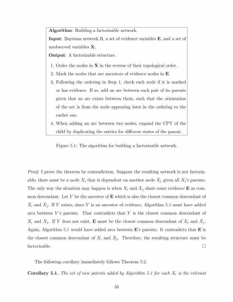
Algorithm: Building a factorizable network.
Input: Bayesian network B, a set of evidence variables E, and a set of
unobserved variables X;
Output: A factorizable structure.
1. Order the nodes in X in the reverse of their topological order.
2. Mark the nodes that are ancestors of evidence nodes in E.
3. Following the ordering in Step 1, check each node if it is marked
or has evidence. If so, add an arc between each pair of its parents
given that no arc exists between them, such that the orientation
of the arc is from the node appearing later in the ordering to the
earlier one.
4. When adding an arc between two nodes, expand the CPT of the
child by duplicating the entries for different states of the parent.
Figure 5.1: The algorithm for building a factorizable network.
Proof. I prove the theorem by contradiction. Suppose the resulting network is not factoriz-
able, there must be a node Xi that is dependent on another node Xj given all Xi’s parents.
The only way the situation may happen is when Xi and Xj share some evidence E as com-
mon descendant. Let Y be the ancestor of E which is also the closest common descendant of
Xi and Xj. If Y exists, since Y is an ancestor of evidence, Algorithm 5.1 must have added
arcs between Y ’s parents. That contradicts that Y is the closest common descendant of
Xi and Xj. If Y does not exist, E must be the closest common descendant of Xi and Xj.
Again, Algorithm 5.1 would have added arcs between E’s parents. It contradicts that E is
the closest common descendant of Xi and Xj. Therefore, the resulting structure must be
factorizable.
The following corollary immediately follows Theorem 5.2.
Corollary 5.1. The set of new parents added by Algorithm 5.1 for each Xi is the relevant
50

factor of Xi, i.e., RF(Xi).
Algorithm 5.1 is similar to the graph reduction method proposed in (Olmsted 1983;
Shachter 1990). Indeed, my procedure will introduce the same additional arcs as the graph
reduction method if two methods use the same ordering. However, the difference is that
graph reduction absorbs the evidence while reducing the graph, which, in the end, results
in a new network without evidence variables. In my procedure, I separate graph reduction
and evidence absorption. We first create a new network that still represents the same distri-
bution as the original one. Given the new structure, we can factorize the full joint posterior
distribution using chain rule and absorb evidence into each CPT separately. Ortiz (2001)
presents a similar idea for constructing an optimal importance function, in which he suggests
first triangulating the Bayesian network and making it chordal, and then constructing the
new structure from the chordal graph. My approach avoids his intermediate step.
In Step 3 of Algorithm 5.1, we add arcs between all the parents of a node if they do
not already exist. Hence, the last parent will get arcs coming from all the other parents.
If the CPT size of the last parent is initially large, or if there are many parents, the new
CPT for the last parent may blow up. Even if not, the new structure will make importance
sampling inefficient. To remedy the problem, I propose several heuristics for preprocessing
the ordering of the parents. All the heuristics are subject to the partial constraints of the
original network, which include arcs or directed paths that already exist among parents.
The first method is to order the parents in the descending order of the number of their own
parents. By doing so, we are trying to make the last parent have as less incoming arcs as
possible, which can reduce the size of the CPTs. The second method is to order the parents
in a descending order of the size of their CPTs. Since our purpose is to minimize the size
of CPTs, the second heuristic is more effective. I will use it in all the experiments in this
chapter.
51

5.2 APPROXIMATION STRATEGIES FOR THE IMPORTANCE
FUNCTIONS
From Equation 5.4, we can see that to build a factorizable structure, we need to add many
arcs to the new structure when we have diagnostic evidence. These extra arcs make a network
much more complex and make the calculation of the CPTs much more difficult. Although I
proposed several heuristics for minimizing the size of CPTs, they can still grow too large. In
fact, this process is practically equivalent to exact inference in the network. Therefore, we
usually only use approximations of the full factorizable structures. Here I will review several
approximation strategies used by the existing importance sampling algorithms for Bayesian
networks. I will use a running example to illustrate these strategies.
Example: A simple Bayesian network with three binary variables in Figure 5.2 param-
eterized as follows:
a 0.2
¬a 0.8
b 0.7
¬b 0.3
a ¬a
P (C|A,B) b ¬b b ¬b
c 0.99 0.01 0.1 0.9
¬c 0.01 0.99 0.9 0.1
µ´¶³
µ´¶³µ´
¶³
@@R
A B
C
Figure 5.2: A simple Bayesian network.
Variable C is observed in state ¬c. We can easily calculate the posterior joint distribution
over A and B.
52

P (A,B|¬c) a ¬a
b 0.0024 0.8560
¬b 0.1009 0.0408
¤Original CPT-based Importance Function: Probabilistic logic sampling (Henrion
1988) assumes that the importance function has the same CPTs as the original network for
all the variables. Likelihood weighting (Fung and Chang 1989; Shachter and Peot 1989) goes
a step further and assumes that the importance function has the following form:
P (X|E) =n∏
i=1
P (Xi|PA(Xi)\E.E ∩ PA(Xi)) (5.5)
It uses the same CPTs as the original distribution for nodes with no evidence parents.
Otherwise, it shrinks CPTs for those nodes with evidence parents. Obviously, this approxi-
mation only takes into account the primitive influence of the evidence, the influence of the
evidence nodes on the CPTs of their children. As you can see from the running example,
original CPT-based importance function is far away from the actual posterior distribution.
Example: Original CPT-based importance function for the running example.
P (A,B) a ¬a
b 0.14 0.56
¬b 0.06 0.24
¤ICPT-based Importance Function: Several algorithms notice the limitations of the
importance function used by likelihood weighting and propose a different form of importance
function. They still assume the same structure for the importance function as the original
Bayesian network, but they realize that the evidence has influence on the CPTs of all the
nodes and propose the following form of importance function:
P (X|E) =n∏
i=1
P (Xi|PA(Xi)\E,E). (5.6)
53
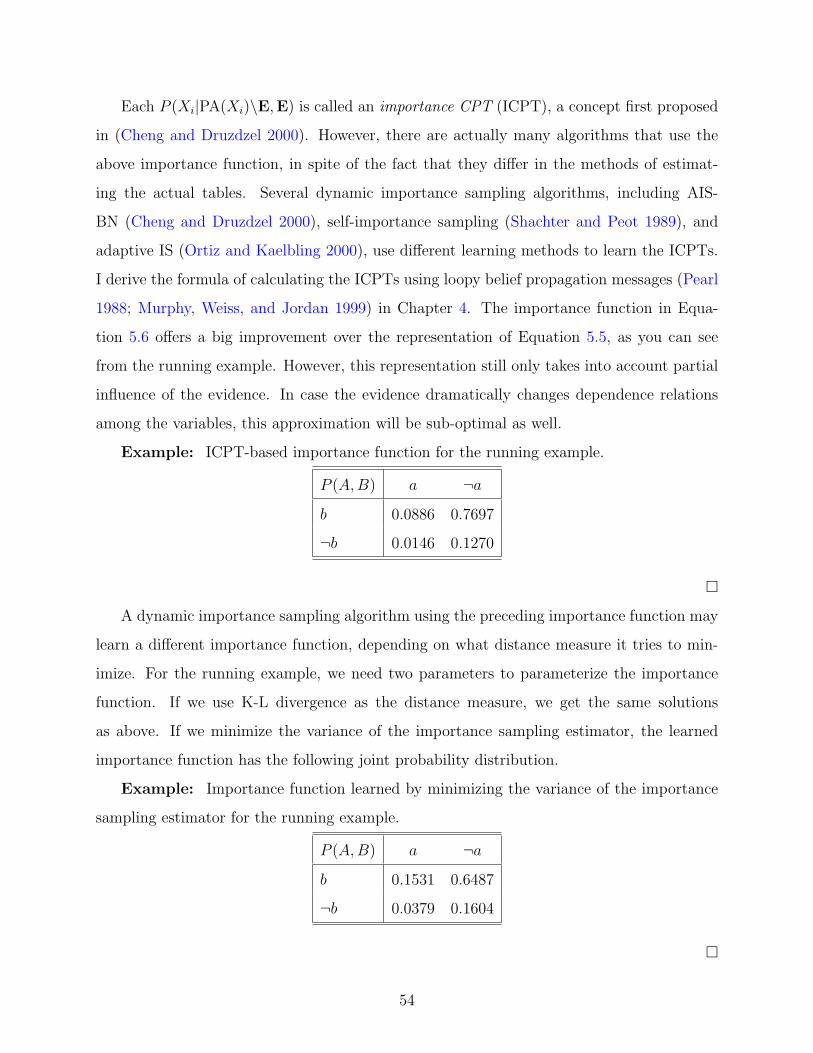
Each P (Xi|PA(Xi)\E,E) is called an importance CPT (ICPT), a concept first proposed
in (Cheng and Druzdzel 2000). However, there are actually many algorithms that use the
above importance function, in spite of the fact that they differ in the methods of estimat-
ing the actual tables. Several dynamic importance sampling algorithms, including AIS-
BN (Cheng and Druzdzel 2000), self-importance sampling (Shachter and Peot 1989), and
adaptive IS (Ortiz and Kaelbling 2000), use different learning methods to learn the ICPTs.
I derive the formula of calculating the ICPTs using loopy belief propagation messages (Pearl
1988; Murphy, Weiss, and Jordan 1999) in Chapter 4. The importance function in Equa-
tion 5.6 offers a big improvement over the representation of Equation 5.5, as you can see
from the running example. However, this representation still only takes into account partial
influence of the evidence. In case the evidence dramatically changes dependence relations
among the variables, this approximation will be sub-optimal as well.
Example: ICPT-based importance function for the running example.
P (A,B) a ¬a
b 0.0886 0.7697
¬b 0.0146 0.1270
¤A dynamic importance sampling algorithm using the preceding importance function may
learn a different importance function, depending on what distance measure it tries to min-
imize. For the running example, we need two parameters to parameterize the importance
function. If we use K-L divergence as the distance measure, we get the same solutions
as above. If we minimize the variance of the importance sampling estimator, the learned
importance function has the following joint probability distribution.
Example: Importance function learned by minimizing the variance of the importance
sampling estimator for the running example.
P (A,B) a ¬a
b 0.1531 0.6487
¬b 0.0379 0.1604
¤
54

We can see that we cannot achieve the optimal importance function by learning. The
reason is that the actual posterior distribution typically needs more parameters to param-
eterize than the importance function. For the running example, the actual posterior dis-
tribution needs three parameters. Obviously, it is in general impossible to perfectly fit a
three-parameter distribution with a two-parameter distribution.
Variable Elimination-based Importance Function: Hernandez et al. (Hernandez,
Moral, and Salmeron 1998) propose to use the variable elimination (Zhang and Poole 1994)
algorithm to eliminate the variables one by one in order to get the CPTs. If the calculation is
carried out exactly, they will get the exact form of the importance function as in Equation 5.4.
However, variable elimination is infeasible for large complex networks. Therefore, they set
a threshold to the CPT size. Whenever the size of a CPT generated when eliminating a
variable exceeds the threshold, they generate multiple smaller tables to approximate the
single big table. Therefore, there is no explicit form for their importance function.
For the simple running example, since variable elimination can be carried out exactly,
Hernandez et al.’s method is able to generate the exact CPTs.
Example: Variable Elimination-based importance function for the running example. If
we eliminate B before A, we get conditional forms P (A) and P (B|A), which are
a 0.1033
¬a 0.8967
P (B|A) a ¬a
b 0.0232 0.9545
¬b 0.9768 0.0455
¤A simple calculation shows that the importance function is indeed equivalent to the
actual posterior distribution. However, for larger models, variable elimination-based impor-
tance function often need to use several tables to approximate a single big table. Since the
approximation is driven mostly by table size, the approximation can be also sub-optimal.
Salmeron et al. (Salmeron, Cano, and Moral 2000) later propose to improve the approxima-
55

tion using probability trees to represent the CPTs.
5.3 AN INFLUENCE-BASED APPROXIMATION STRATEGY FOR
IMPORTANCE FUNCTIONS
In the previous section, I argue that some existing approximations cannot approximate the
posterior distribution well. I now begin to discuss one approximation strategy that is based
on the influence among variables in a Bayesian network introduced by the evidence.
First, I provide an analysis of the influence of evidence. We know that in general di-
agnostic evidence makes the ancestors of evidence nodes conditionally dependent. We need
to model the most important dependence relations in order to obtain a good importance
function. One useful measure to model the relative strength of the dependence relations
among the variables in a Bayesian network is the sensitivity range of the probability of an
event y with respect to an event x (Henrion 1989). More formally, suppose that E = e is the
observed evidence which might affect the assessment of the probability of x, giving P (x|e).Suppose that Y is conditionally independent of E given X. Then the sensitivity range is
defined as the derivative of P (y|e) with respect to P (x|e):
SR(y, x) ≡ ∂P (y|e)∂P (x|e) . (5.7)
Henrion (1989) has shown that for the causal link in Figure 5.3, the sensitivity range
SR(y, x) with respect to e satisfies the following inequality:
|SR(y, x)| ≤ 1. (5.8)
Essentially, the result shows that the evidence on a node has more influence on its im-
mediate children than its further descendants. Now, I extend the result to more general
scenarios. First, let us look at the diagnostic link in Figure 5.4. Given conditional indepen-
dence, P (y|x) = P (y|x, e). We have
P (y|e) = P (y|x)P (x|e) + P (y|¬x)(1− P (x|e)) . (5.9)
56

µ´¶³
µ´¶³
µ´¶³@@R
-
E
X Y
Figure 5.3: A causal link.
µ´¶³
µ´¶³
µ´¶³@@I
E
X Y
Figure 5.4: A diagnostic link.
Taking the derivative with respect to P (x|e), we get
SR(y, x) = P (y|x)− P (y|¬x) . (5.10)
Obviously, Equation 5.8 also holds for the diagnostic link. It shows that the evidence on
a node has more influence on its immediate parents than its further ancestors. Now, let us
look at a more interesting case. Suppose we have an intercausal network as in Figure 5.5,
we have
µ´¶³
µ´¶³
µ´¶³
µ´¶³
@@I
E
X Y
Z
Figure 5.5: An intercausal link.
P (y|z, e) = P (y|x)P (x|z, e) + P (y|¬x)(1− P (x|z, e)) . (5.11)
57

Taking the derivative with respect to P (x|z, e), we get
SR(y, x) = P (y|x)− P (y|¬x) . (5.12)
Again, Equation 5.8 holds for this case. This result shows that, although an evidence
node introduces dependence among its ancestors, the strength of the dependence will become
weaker as the distance between the ancestors increases.
To summarize, my discussion essentially shows that, in general, as the distance from
a variable to the evidence becomes larger in a Bayesian network, the evidence usually has
less influence on the posterior distribution of the variable. Also, the dependence relations
among the immediate parents of an evidence node are stronger than those among its further
ancestors. Similarly, we can show the same results using another dependence measure called
mutual information.
For each CPT P (Xi|PA(Xi),E, RF(Xi)) in Equation 5.4, PA(Xi) are immediate parents
of Xi, so their influence are usually strong. E contains the observed variables, so it only
reduces the complexity of the CPT. However, the variables in RF(Xi) have varying distances
from Xi. From the analysis, I believe that by throwing away the variables that are further
away from Xi, I can still reserve a good approximation of the original CPT. Therefore, I
propose to approximate the full importance function by adding additional arcs only among
the parents of evidence. By modelling the most important additional dependence among the
variables, I anticipate that the importance function can be quite close to the actual posterior
distribution. Keeping adding arcs makes the network more complex, which may only bring
minimal improvement but makes the computation more costly.
5.4 EXPERIMENTAL RESULTS
To justify my proposed approximation strategy, I tested it on the EPIS-BN algorithm. I
performed my experiments on the ANDES (Conati, Gertner, VanLehn, and Druzdzel 1997),
CPCS (Pradhan, Provan, Middleton, and Henrion 1994), and PathFinder (Heckerman
1990) networks. My comparison was based on the average Hellinger’s distance (Kokolakis
58

and Nanopoulos 2001) between exact posterior marginals of all unobserved variables and
sampling results.
5.4.1 Results of Different Representations on ANDES
In this experiment, I generated a total of 75 test cases for the ANDES network. These
cases consisted of five sequences of 15 cases each. For each sequence, I randomly chose
a different number of evidence nodes: 15, 20, 25, 30, 35 respectively. I used three different
representations of importance function in this experiment. The first one was represented by
ICPTs, as in Equation 5.6. For the second one, I only added additional arcs between the
parents of the evidence nodes. For the third one, I carried out Algorithm 5.1 fully and added
all the necessary arcs to make the network factorizable. I then ran EPIS-BN on the three
importance functions. The results are shown in Figure 5.6.
As we can see, adding arcs between the parents of evidence nodes brings immediate
reduction in error. A paired one-tail t-test at p = 0.00029 level shows that the improvement
is significant. Since the new importance function has few new arcs, its influence on the
running time was minimal. Adding more arcs to get the exact importance function form did
not improve the results, but only made the algorithm less efficient. P-value in this case is
0.0018. The results clearly agree with my analysis of the influence of evidence.
5.4.2 Results of Different Representations on CPCS and PathFinder
In this experiment, I used the same experimental setup and did some experiments on the
CPCS and PathFinder networks. The results are shown in Figure 5.7. Again, adding arcs
among the parents of evidence nodes brings immediate improvements for EPIS-BN. Adding
more arcs to get the exact importance function form did not improve the results, but only
made the algorithm less efficient.
59
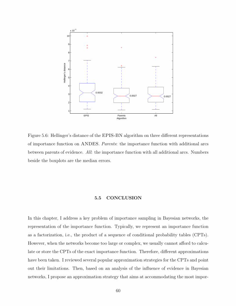
EPIS Parents All
1
2
3
4
5
6
7
8
9
10
x 10−3
Hel
linge
r’s d
ista
nce
Algorithm
0.0032 0.0027 0.0027
Figure 5.6: Hellinger’s distance of the EPIS-BN algorithm on three different representations
of importance function on ANDES. Parents: the importance function with additional arcs
between parents of evidence. All: the importance function with all additional arcs. Numbers
beside the boxplots are the median errors.
5.5 CONCLUSION
In this chapter, I address a key problem of importance sampling in Bayesian networks, the
representation of the importance function. Typically, we represent an importance function
as a factorization, i.e., the product of a sequence of conditional probability tables (CPTs).
However, when the networks become too large or complex, we usually cannot afford to calcu-
late or store the CPTs of the exact importance function. Therefore, different approximations
have been taken. I reviewed several popular approximation strategies for the CPTs and point
out their limitations. Then, based on an analysis of the influence of evidence in Bayesian
networks, I propose an approximation strategy that aims at accommodating the most impor-
60

EPIS Parents All
0.5
1
1.5
2
2.5
3
3.5
4
4.5
x 10−3
Hel
linge
r’s d
ista
nce
Algorithm
0.00077 0.00074 0.00074
EPIS Parents All
0.5
1
1.5
2
2.5
3
3.5
4
4.5
5
5.5
x 10−3
Hel
linge
r’s d
ista
nce
Algorithm
0.00074 0.00072 0.00072
(a) (b)
Figure 5.7: Hellinger’s distance of the EPIS-BN algorithm on three different representations
of importance function on (a) CPCS and (b) PathFinder.
tant additional dependence introduced by the evidence. The proposed importance function
is easier to interpret. My experimental results also show that the new approximation strat-
egy offers an immediate improvement of the quality of the importance function and almost
the same performance as the full factorizable structures. However, there were two approx-
imations happened during the experiment. We not only approximated the representations
of the importance functions, but also used an approximate algorithm, LBP, to calculate the
actual functions. In my future work, I plan to perform extra experiments to disambiguate
the effect of the two approximations. Also, by introducing more parameters, the improved
importance function form also brings much potential for dynamic sampling algorithms, as
they can learn theoretically better importance functions.
61

6.0 HYBRID LOOPY BELIEF PROPAGATION
This dissertation so far has been focusing on discrete Bayesian networks. As Bayesian
networks (BNs) (Pearl 1988) are applied to more practical domains, people realize that
some problems are more naturally represented by hybrid Bayesian networks that contain
mixtures of discrete and continuous variables. However, several factors make inference in
hybrid models extremely hard. First, they may include linear and non-linear deterministic
relations. Second, the models may contain arbitrary probability distributions. Third, the
orderings among the discrete and continuous variables may be arbitrary. Actually it has been
shown that inference is NP-hard even for the simplest parametric case, the CLG tree (Lerner
and Parr 2001).
Since the general case is difficult, the earliest attempts to model continuous variables fo-
cused on special instances of hybrid models, such as Conditional Linear Gaussians (CLG) (Lau-
ritzen 1992). CLG received much attention because it has a nice property: we can calculate
exactly the first two moments for the posterior probability distributions of the continuous
variables and the exact posterior probability distributions for the discrete variables. How-
ever, one major assumption behind CLG is that discrete variables cannot have continuous
parents. This limitation was later addressed by extending CLG with logistic and softmax
functions (Lerner, Segal, and Koller 2001; Murphy 1999). These attempts raised much in-
terest in hybrid Bayesian networks, especially in developing methodologies for more general
non-Gaussian models, such as Mixture of Truncated Exponentials (MTE) (Cobb and Shenoy
2005; Moral, Rumi, and Salmeron 2001), and junction tree algorithm with approximate clique
potentials (Koller, Lerner, and Angelov 1999). Most of these approaches rely on the junction
tree algorithm (Lauritzen and Spiegelhalter 1988). However, as Lerner et al. (Lerner, Segal,
and Koller 2001) pointed out, it is important to have alternative solutions in the case that
62

junction tree algorithm-based methods are not feasible.
In this chapter, I propose the Hybrid Loopy Belief Propagation (HLBP) algorithm, which
extends the Loopy Belief Propagation (LBP) (Murphy, Weiss, and Jordan 1999) and Nonpara-
metric Belief Propagation (NBP) (Sudderth, Ihler, Freeman, and Willsky 2003) algorithms
to deal with general hybrid Bayesian networks. The main idea is to represent each LBP
message as a Mixture of Gaussians (MG) and formulate its calculation as a Monte Carlo in-
tegration problem. The extension is far from trivial due to the enormous complexity brought
by deterministic equations and mixture of discrete and continuous variables. Another ad-
vantage of the algorithm is that it approximates the true posterior probability distributions,
unlike most existing approaches which only produce the first two moments for CLG models.
I also propose a technique called lazy LBP, which can significantly improve the efficiency of
LBP and related methods.
I depart this chapter a little from importance sampling, the main theme of this dis-
sertation, because I believe that HLBP itself is an important method for hybrid Bayesian
networks. I will investigate how to use the HLBP algorithm to calculate importance functions
for importance sampling in the next chapter.
The remainder of this chapter is structured as follows. In Section 6.1, I propose the Hybrid
Loopy Belief Propagation (HLBP) algorithm and discuss how to calculate LBP messages
in hybrid Bayesian networks. Section 6.2 discusses an efficient method to sample from a
product of several mixtures of Gaussians. Section 6.3 discusses how to deal with evidence
and deterministic relations in HLBP. In Section 6.4, I propose a technique that I call Lazy
LBP to improve the efficiency of HLBP. Finally in Section 6.5, I present some experimental
results.
6.1 HYBRID LOOPY BELIEF PROPAGATION
To extend LBP to hybrid Bayesian networks, we need to know how to calculate the messages.
It is evident that no closed-form solutions exist for the messages in general hybrid models.
However, I observe that their calculations can be formulated as Monte Carlo integration
63

problems. Since we are dealing with mixtures of discrete and continuous variables, we will
have integrations and summations mixed together. For simplicity, I will only use integrations
in the message definitions.
First, let us look at the π(t+1)Yj
(x) message defined in Equation 4.7. I plug in the definition
of π(t)(x) in Equation 4.5 and rearrange the equation in the following way:
π(t+1)Yj
(x)
= αλX(x)∏
k 6=j
λ(t)Yk
(x)
∫
u
P (x|u)∏
k
π(t)X (uk)
= α
∫
u
P (x,u)︷ ︸︸ ︷λX(x)
∏
k 6=j
λ(t)Yk
(x)P (x|u)∏
k
π(t)X (uk)
.
Essentially, I put all the integrations outside of the other operations. Given the new
formula, I realize that I have a joint probability distribution over x and uis, and the task is
to integrate all the uis out and get the marginal probability distribution over x. Since P (x, u)
can be naturally decomposed into P (x|u)P (u) for this message, calculating the message can
be solved using a Monte Carlo sampling technique called Composition method (Tanner 1993).
The idea is first to draw samples for each uis from π(t)X (ui), and then sample from the product
of λX(x)∏k 6=j
λ(t)Yk
(x)P (x|u). I will discuss how to take the product in the next subsection. For
now let us assume that the computation is possible. To make life even easier, I make further
modifications and get
π(t+1)Yj
(x)
= α
∫
u
λX(x)∏k
λ(t)Yk
(x)P (x|u)∏k
π(t)X (uk)
λ(t)Yj
(x)
.
Now, for the messages sent from X to its different children, we can share most of the calcu-
lation. We first get samples for uis and then sample from the product of λX(x)∏k
λ(t)Yk
(x)P (x|u).
For each different message π(t+1)Yj
(x), we use the same sample x but assign it different weights
1/λ(t)Yi
(x).
64

Let us now consider how to calculate the λ(t+1)X (ui) message defined in Equation 4.6. First,
I plug in the definition of λ(t)(x) in Equation 4.4 and rearrange the equation analogously:
λ(t+1)X (ui)
= α
∫
x
λX(x)∏
j
λ(t)Yj
(x)
∫
uk:k 6=i
P (x|u)∏
k 6=i
π(t)X (uk)
= α
∫
x,uk:k 6=i
P (x,uk:k 6=i|ui)︷ ︸︸ ︷λX(x)
∏j
λ(t)Yj
(x)P (x|u)∏
k 6=i
π(t)X (uk)
. (6.1)
It turns out that here we are facing a quite different problem from the calculation of
π(t+1)Yj
(x). Note now we have P (x, uk : k 6= i|ui), a joint distribution over x and uk(k 6= i)
conditional on ui, so the whole expression is only a likelihood function of ui, which is not
guaranteed to be integrable. As in (Sudderth, Ihler, Freeman, and Willsky 2003; Koller,
Lerner, and Angelov 1999), I choose to restrict my attention to densities and assume that
the ranges of all continuous variables are bounded (maybe large). The assumption only solves
part of the problem. Another difficulty is that composition method is no longer applicable
here, because we have to draw samples for all parents ui before we can decide P (x|u). I
note that for any fixed ui, Equation 6.1 is an integration over x and uk, k 6= i. The integral,
complex as it is, can be carried out using Monte Carlo methods. Therefore, we can evaluate
λ(t+1)X (ui) up to a constant for any value ui, although we do not know how to sample from
it. This is exactly the time when importance sampling becomes handy. We can estimate the
message by drawing a set of samples as follows: we sample for ui from a chosen importance
function, evaluate λ(t+1)X (ui) using Monte Carlo integration, and take ratio between the final
value and I(ui) as the weight for this sample. A simple choice for the importance function is
the uniform distribution over the range of ui, but we can improve the accuracy of Monte Carlo
integration by choosing a more informed importance function, the corresponding message
λ(t)X (ui) from the last iteration. Because of the iterative nature of LBP, messages usually
keep improving over each iteration, so they are clearly better importance functions. More
65

formally, I am essentially rearranging Equation 6.1 as follows.
λ(t+1)X (ui)
= α
∫
x,uk:k 6=i
λX(x)∏j
λ(t)Yj
(x)P (x|u)λ(t)X (ui)
∏k 6=i
π(t)X (uk)
λ(t)X (ui)
.
Now we know how to use Monte Carlo integration methods to calculate the messages
for LBP, represented as sets of weighted samples. To complete the algorithm, we need to
figure out how to propagate these messages. That involves operations like sampling, multi-
plication, and marginalization. Sampling from a message represented as a set of weighted
samples may be easy to do; we can use resampling technique to achieve that. However,
multiplying two such messages is not straightforward. Therefore, I choose to use density
estimation techniques to approximate each continuous message using a mixture of Gaus-
sians (MG) (Sudderth, Ihler, Freeman, and Willsky 2003). A K component mixture of
Gaussian has the following form
M(x) =K∑
i=1
wiN(x; µi, σi) , (6.2)
whereK∑
i=1
wi = 1. MG has several nice properties. First, we can approximate any continuous
distribution reasonably well using a MG. Second, it is closed under multiplication. Last, we
can estimate a MG from a set of weighted samples using a regularized version of expectation
maximization (EM) (Dempster, Laird, and Rubin 1977; Koller, Lerner, and Angelov 1999)
algorithm.
Given the above discussion, I outline the final HLBP algorithm in Figure 6.1. I first
initialize all the messages. Then, I iteratively recompute all the messages using the Monte
Carlo methods described above. In the end, I calculate the messages λ(x) and π(x) for each
node X and use them to estimate the posterior probability distribution over X.
66

Algorithm: HLBP
1. Initialize the messages that evidence nodes send to themselves and
their children as indicating messages with fixed values, and initialize
all other messages to be uniform.
2. while (stopping criterion not satisfied)
Recompute all the messages using Monte Carlo
integration methods.
Normalize discrete messages.
Approximate all continuous messages using MGs.
end while
3. Calculate λ(x) and π(x) messages for each variable.
4. Calculate the posterior probability distribution for all the variables
by sampling from the product of λ(x) and π(x) messages.
Figure 6.1: The Hybrid Loopy Belief Propagation (HLBP) algorithm.
67

6.2 PRODUCT OF MIXTURES OF GAUSSIANS
One question that remains to be answered in the last section is how to sample from the
product of λX(x)∏k 6=j
λ(t)Yk
(x)P (x|u). I address the problem in this section. If P (x|u) is
a continuous probability distribution, we can approximate P (x|u) with a MG. Then, the
problem becomes how to compute the product of several MGs. The approximation is often a
reasonable thing to do because we can approximate any continuous probability distribution
reasonably well using MG. Even when such approximation is poor, we can approximate
the product of P (x|u) with an MG using another MG. One example is that the product of
Gaussian distribution and logistic function can be approximated well with another Gaussian
distribution (Murphy 1999).
Suppose we have messages M1,M2, ..., MK , each represented as an MG. Since MG is
closed under multiplication, a straightforward solution is to explicitly carry out the product
and get a single final MG in the end. Sampling from the final MG becomes trivial. However,
this method will easily produce a MG with a huge number of Gaussian components. Assum-
ing each message has N components, the final MG would have NK components. This is not
desirable for an iterative algorithm like HLBP. Another approach to do the multiplication is
to use importance sampling. We can randomly pick one component N(x; µiji, σiji
) from each
message Mj according their weights, multiply them into a single Gaussian N(x; µ∗K , σ∗K),
and draw a sample from the final Gaussian. However, we have to assign each sample the
following weight
w =
K∏i=1
N(x; µiji, σiji
)
N(x; µ∗K , σ∗K).
The weight comes up because the product of Gaussians is only proportional to another
Gaussian. Sudderth et al. use Gibbs sampling algorithm to address the problem (Sudderth,
Ihler, Freeman, and Willsky 2003). The idea is based on the observation that a sample
from the whole product must be a sample from one component in the final MG, which is
a product of K Gaussians, one from each MG message. If we treat the selection of one
component from each MG message as a random variable, which we call a label, we can use
Gibbs sampling to draw a sample from the joint probability distribution of all the labels
68

P (L1, L2, ..., LK). We then use the sample to select the Gaussian components, multiply
them into a single Gaussian, and draw a sample from it. The shortcoming of the Gibbs
sampler is its efficiency: We usually have to carry out several iterations of Gibbs sampling
in order to get one sample.
Here, I propose a more efficient method to draw importance samples from a product of
MGs. The idea originates from the chain rule. I note that the joint probability distribution
of the labels of all the messages P (L1, L2, ..., LK) can be factorized using the chain rule as
follows:
P (L1, L2, ..., LK) = P (L1)K∏
i=2
P (Li|L1, ..., Li−1) . (6.3)
Therefore, the idea is to sample from the labels sequentially based on the prior or condi-
tional probability distributions. Let wij be the weight for the jth component of ith message
and µij and σij be the component’s parameters. We can sample from the product of mes-
sages M1, ...,MK using the algorithm presented in Figure 6.2. The main idea is to calculate
the conditional probability distributions cumulatively. Due to the Gaussian densities, the
method has to correct its bias introduced during the sampling by assigning the samples
weights. The method only needs to go over the messages once to obtain an importance
sample and is much more efficient than the Gibbs sampler in (Sudderth, Ihler, Freeman,
and Willsky 2003). Empirical results show that the precision obtained by the importance
sampler is comparable to the Gibbs sampler given a reasonable number of samples.
6.3 BELIEF PROPAGATION WITH EVIDENCE
Special care is needed for belief propagation with evidence and deterministic relations. In my
previous discussions, I approximate P (x|u) using MG if P (x|u) is a continuous probability
distribution. It is not the case if P (x|u) is deterministic or if X is observed. I discuss the
following several scenarios separately.
Deterministic relation without evidence: I simply evaluate P (x|u) to get the value x as
a sample. Because I did not take into account the λ messages, I need to correct the bias by
weighting samples. For the message πYi(x) sent from X to its child Yi, I take x as the sample
69

Algorithm: Sample from a product of MGs M1 ×M2 × ...×MK .
1. Randomly pick a component, say j1, form the first message M1
according to its weights w11, ..., w1J1 .
2. Initialize cumulative parameters as follows
µ∗1 ← µ1j1 ; σ∗1 ← σ1j1 .
3. i ← 2; wImportance ← w1j1 .
4. while (i ≤ K)
Compute new parameters for each component of ith message as
follows
σ∗ik ← ((σ∗i−1)−1 + (σik)
−1)−1,
µ∗ik ← (µik
σik+
µ∗i−1
σ∗i−1)σ∗ik.
Compute new weights for ith message with any x
w∗ik = wikw
∗i−1ji−1
N(x;µ∗i−1,σ∗i−1)N(x;µik,σik)
N(x;µ∗ik,σ∗ik).
Calculate the normalized weights w∗ik.
Randomly pick a component, say ji, from the ith message using
the normalized weights.
Let µ∗i ← µ∗iji; σ∗i ← σ∗iji
.
i ← i + 1;
wImportance = wImportance× w∗iji
.
end while
5. Sample from the Gaussian with mean µ∗K and variance σ∗K .
6. Assign the sample weight w∗KjK
/wImportance.
Figure 6.2: An importance sampler for sampling from a product of MGs.
and assign it weight λX(x)∏k 6=i
λ(t)Yk
(x). For the message λX(ui) sent from X to its parent Ui,
I take value ui as a sample for Ui and assign it weight λX(x)∏k
λ(t)Yk
(x)/λ(t)X (ui).
70

Stochastic relation with evidence: The messages πYj(x) sent from evidence node X to its
children are always indicating messages with fixed values. The messages λYj(x) sent from
the children to X have no influence on X, so I need not calculate them. I only need to
update the messages λX(ui), for which I take the value ui as the sample and assign it weight
λX(e)∏k
λ(t)Yk
(e)/λ(t)X (ui), where e is the observed value of X.
Deterministic relation with evidence: This case is the most difficult. To illustrate it more
clearly, I use a simple hybrid Bayesian network with one discrete node A and two continuous
nodes B and C (see Figure 6.3).
Example: ¤
a 0.7
¬a 0.3
B
N(B; 1, 1)
P (C|A,B) a ¬a
C C = B C = 2 ∗B
µ´¶³
µ´¶³µ´
¶³
@@R
A B
C
Figure 6.3: A simple hybrid Bayesian network.
Let C be observed at state 2.0. Given the evidence, there are only two possible values for
B: B = 2.0 when A = a, and B = 1.0 when A = ¬a. We need to calculate messages λC(a)
and λC(b). If we follow the routine and sample from A and B first, it is extremely unlikely
for us to hit a feasible sample; Almost all the samples that we get would have weight 0.0.
Clearly we need a better way to do that.
First, let us consider how to calculate the message λC(a) sent from C to A. Suppose we
choose uniform distribution as the importance function, we first randomly pick a state for
A. After the state of A is fixed, we can solve P (C|A,B) to get the state for B and assign
71

N(B; 1, 1) as the weight for the sample. Since A’s two states are equally likely, the message
λC(A) would be proportional N(2; 1, 1), N(1; 1, 1).For the message λC(b) message sent from C to B, since we know that B can only take
two values, we choose a distribution that puts equal probabilities on these two values as the
importance function for sampling B. Not that the state of B will also determine A as follows:
when B = 2, we have A = a; when B = 1, we have A = ¬a. We then assign weight 0.7 to
the sample if B = 2 and 0.3 if B = 1. However, the magic of knowing feasible values for B
does not happen often in practice. Instead, we can first sample for A from πC(A), 0.7, 0.3.Given the value of A, we can solve P (C|A,B) for B and assign each sample weight 1.0. So
λC(b) have probabilities proportional to 0.7, 0.3 on two values 2.0 and 1.0.
To generalize, in order to calculate λ messages sent out from a deterministic node with
evidence, we need to sample from all parents except one, and then solve P (x|u) for the
remaining parent. There are several issues that we need to consider here. First, since we
want to use the values of other parents to solve for the chosen parent, we need an equation
solver. We used an implementation of the Newton’s method for solving nonlinear set of
equations (Kelley 2003). However, not all equations are solvable by this equation solver or
any equation solver for that matter. We may want to choose the parent that is easiest to
solve. This can be tested by means of a preprocessing step. In more difficult cases, we have
to resort to users’ help and ask at the model building stage for specifying which parent to
solve or even specify the inverse functions manually. When there are multiple choices, one
heuristic that I find helpful is to choose the continuous parent with the largest variance.
6.4 LAZY LBP
We can see that HLBP involves repeated density estimation and Monte Carlo integration,
which are both computationally intense. Efficiency naturally becomes a concern for the
algorithm. To improve its efficiency, I propose a technique called Lazy LBP, which is also
applicable to other extensions of LBP.
After evidence is introduced in the network, we can pre-propagate the evidence to reduce
72

computation in HLBP. First, we can plug in any evidence to the conditional relations of its
children, so we need not calculate the π messages from the evidence to its children any
more. Similarly, we need not calculate the λ messages from its children to the evidence
either. Secondly, evidence may determine the value of its neighbors because of deterministic
relations, in which case we can evaluate the deterministic relations in advance so that we
need not calculate messages between them.
Furthermore, from the definitions of the LBP messages, we immediately have the follow-
ing results.
Theorem 6.1. The λ(x) messages from the children of a node with no evidence as descendant
are always uniform.
Theorem 6.2. A message needs not be updated if the sender of the message has received no
new messages from its neighbors other than the recipient of the message.
Based on Equation 4.6, λ messages should be updated if incoming π messages change.
However, I have the following result.
Theorem 6.3. The λ messages sent from a non-evidence node to its parents remain uniform
before it receives any non-uniform messages from its children, even though there are new π
messages coming from the parents.
Proof. Since there are no non-uniform λ messages coming in, Equation 4.6 simplifies to
λ(t+1)X (ui) = α
∫
x,uk:k 6=i
P (x|u)∏
k 6=i
π(t)X (uk)
= α
∫
x,uk:k 6=i
P (x, uk : k 6= i|ui)
= α .
Finally for HLBP, we may be able to calculate some messages exactly. For example,
suppose a discrete node has only discrete parents. We can always calculate the messages
sent from this node to its neighbors exactly. In this case, we should avoid using Monte Carlo
sampling.
73
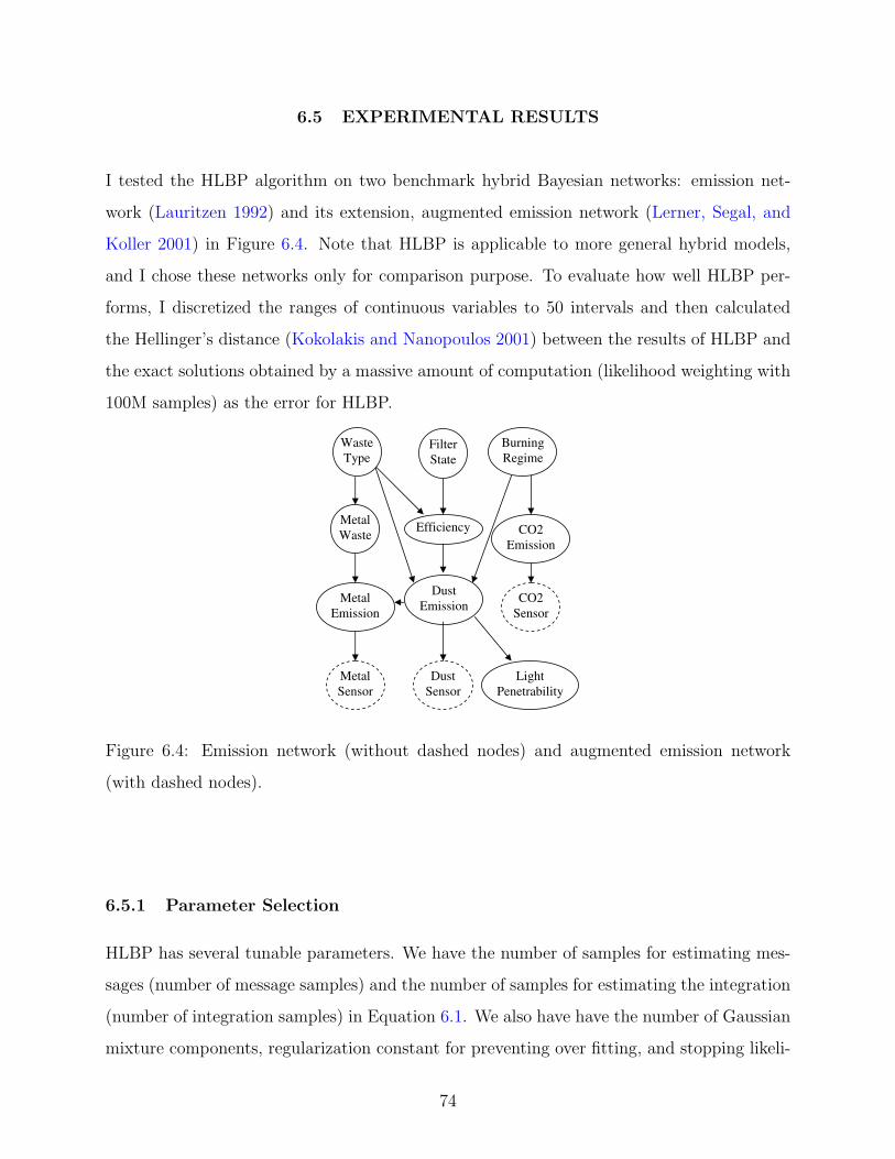
6.5 EXPERIMENTAL RESULTS
I tested the HLBP algorithm on two benchmark hybrid Bayesian networks: emission net-
work (Lauritzen 1992) and its extension, augmented emission network (Lerner, Segal, and
Koller 2001) in Figure 6.4. Note that HLBP is applicable to more general hybrid models,
and I chose these networks only for comparison purpose. To evaluate how well HLBP per-
forms, I discretized the ranges of continuous variables to 50 intervals and then calculated
the Hellinger’s distance (Kokolakis and Nanopoulos 2001) between the results of HLBP and
the exact solutions obtained by a massive amount of computation (likelihood weighting with
100M samples) as the error for HLBP.
Metal
W as teE f f ic ien c y C O 2
E m is s io n
Metal
E m is s io n
D u s t
E m is s io n
L ig h t
P en etrab ility
W as te
T y p e F ilter
S tate
B u r n in g
R eg im e
Metal
S en s o r
D u s t
S en s o r
C O 2
S en s o r
Figure 6.4: Emission network (without dashed nodes) and augmented emission network
(with dashed nodes).
6.5.1 Parameter Selection
HLBP has several tunable parameters. We have the number of samples for estimating mes-
sages (number of message samples) and the number of samples for estimating the integration
(number of integration samples) in Equation 6.1. We also have have the number of Gaussian
mixture components, regularization constant for preventing over fitting, and stopping likeli-
74

hood threshold for the EM algorithm for estimating MGs. The most dramatic influence on
precision comes from the number of message samples, shown as in Figure 6.5(a). Counter
intuitively, the number of message integration samples does not have as big impact as we
might think (see Figure 6.5(b) with 1K message samples). The reason, I believe, is that
when we draw a lot of samples for messages, the precision of each sample becomes less crit-
ical. In my experiments, I set the number of message samples to 1, 000 and the number of
message integration samples to 12. It is also important for the EM algorithm to accurately
approximate the messages using MGs. Therefore, the other parameters also play important
roles. I typically set regularization constant to 0.8, likelihood threshold to 0.001, and the
number of Gaussian mixture components to 2.
0
0.1
0.2
0.3
0.4
0.5
0.6
0.7
1 2 3 4 5 6 7 8 9 1 0
N u m b e r o f M e s s a g e S a m p le s (1 0* 2 ^ (i-1 ))
He
llin
ge
r's D
ista
nce
Im p o rta n c e S a m p le r
G ib b s S a m p le r
0
0.02
0.04
0.06
0.08
0.1
0.1 2
1 2 3 4 5 6 7 8 9 1 0
N u m b e r o f M e s s a g e In te g ra tio n S a m p le s (2 ^ i)
He
llin
ge
r's D
ista
nce
Im p o rta n c e S a m p le r
G ib b s S a m p le r
(a) (b)
Figure 6.5: The influence of (a) the number of message samples and (b) the number of
message integration samples on HLBP on the augmented emission network when observing
CO2Sensor and DustSensor both to be true and Penetrability to be 0.5.
I also compared the performance of two samplers for product of MGs: the Gibbs sam-
pler (Sudderth, Ihler, Freeman, and Willsky 2003) and the importance sampler in Section 6.2.
As we can see from the graph, when the number of message samples is small, Gibbs sam-
pler has slight advantage over the importance sampler. As the number of message samples
increases, the difference becomes negligible. Since the importance sampler is much more
efficient, I use it in all our other experiments.
75

6.5.2 Results on Emission Networks
I note that mean and variance alone, focus of prior work in the field, provide only limited
information about the actual posterior probability distributions. Figure 6.6 shows the pos-
terior probability distribution of node DustEmission when observing CO2Emission at −1.6,
Penetrability at 0.5, and WasteType at 1. I also plotted in the same figure the correspond-
ing normal approximation with mean 3.77 and variance 1.74. We can see that the normal
approximation does not reflect the true posterior. While the actual posterior distribution
has a multimodal shape, the normal approximation does not tell us where the mass really
is. In Figure 6.6, I also plotted the estimated posterior probability distribution of the node
DustEmission by HLBP. HLBP seemed able to estimate the shape of the actual distribution
very accurately.
0
0.2
0.4
0.6
0.8
1
1.2
0.7 6 1.7 2 2 .6 8 3 .6 4 4 .6 5 .5 6 6 .5 2 7 .4 8 8 .4 4
P o s te rio r D is trib u tio n o f D u s tE m is s io n
Pro
babili
ty
E s tim a te d P o s te rio r
E x a c t P o s te rio r
N o rm a l A p p ro x im a tio n
Figure 6.6: Posterior probability distribution of DustEmission when observing CO2Emission
to be −1.6, Penetrability to be 0.5 and WasteType to be 1 on the emission network.
In Figures 6.7(a) and (b), I plot the average error curves of 50 runs of HLBP and Lazy
HLBP (HLBP enhanced by Lazy LBP) as a function of the propagation length. We can see
that HLBP only needs several steps to converge. Furthermore, HLBP achieves better preci-
sion than its lazy version, but Lazy HLBP is much more efficient than HLBP. Theoretically,
Lazy LBP should not affect the precision of HLBP. The reason for the difference between
76

the precision of HLBP and Lazy HLBP is that we use importance sampling to estimate the
messages. Since I use the messages from the last iteration as importance functions, iterations
will help improving the functions. In the case that the messages are calculated exactly, for
example in discrete Bayesian networks, Lazy LBP will improve the efficiency of LBP while
providing the same results.
I also tested the HLBP algorithm on the augmented Emission network (Lerner, Segal, and
Koller 2001) with CO2Sensor and DustSensor both observed to be true and Penetrability to
be 0.5 and report the results in Figures 6.7(c,d). I again observed that not many iterations
are needed for HLBP to converge. In this case, Lazy HLBP provides comparable results
while improving the efficiency of HLBP.
0
0.05
0.1
0.1 5
0.2
0.2 5
0.3
0.3 5
1 2 3 4 5 6 7 8 9 1 0
P ro p a g a tio n L e n g th
He
llin
ge
r's D
ista
nce
H L B P
L a z y H L B P
0
0.5
1
1.5
2
2.5
3
3.5
4
1 2 3 4 5 6 7 8 9 10
P ro p a g a tio n L e n g th
Ru
nn
ing
Tim
e (
s)
H L B P
L a z y H L B P
(a) (b)
0
0.05
0.1
0.1 5
0.2
0.2 5
0.3
0.3 5
1 2 3 4 5 6 7 8 9 1 0
P ro p a g a tio n L e n g th
He
llin
ge
r's D
ista
nce
H L B P
L a z y H L B P
0
1
2
3
4
5
6
7
8
9
10
1 2 3 4 5 6 7 8 9 10
P ro p a g a tio n L e n g th
Ru
nn
ing
Tim
e (
s)
H L B P
L a z y H L B P
(c) (d)
Figure 6.7: Results of HLBP and Lazy HLBP: (a) error on emission, (b) running time on
emission, (c) error on augmented emission, (d) running time on augmented emission.
77

6.6 CONCLUSION
The contribution of this chapter is three-fold. First, I propose the Hybrid Loopy Belief
Propagation (HLBP) algorithm, which extends LBP and NBP to deal with hybrid Bayesian
networks. The algorithm is general enough to deal with linear or nonlinear equations and
arbitrary probability distributions and naturally accommodate the situation where discrete
variables have continuous parents. Another advantage of the algorithm is that it approx-
imates the true posterior probability distributions, unlike most existing approaches which
only produce the first two moments for CLG models. Second, I propose an importance
sampler to sample from a product of MGs, whose accuracy is comparable to the Gibbs sam-
pler in (Sudderth, Ihler, Freeman, and Willsky 2003) given a reasonable number of samples.
Third, I propose a technique called lazy LBP to improve the efficiency of HLBP. Just as
LBP, I anticipate that HLBP will work well for many practical models and can serve as a
promising approximate method for hybrid Bayesian networks. The HLBP algorithm also has
other indirect applications. In the next chapter, I investigate how to use HLBP to calculate
importance functions for importance sampling in hybrid models.
78

7.0 EVIDENCE PRE-PROPAGATED IMPORTANCE SAMPLING
ALGORITHM FOR GENERAL HYBRID BAYESIAN NETWORKS
Many importance sampling-based algorithms have been proposed to deal with inference tasks
in discrete Bayesian networks. Importance sampling algorithms, such as likelihood weight-
ing (LW) (Fung and Chang 1989; Shachter and Peot 1989), AIS-BN (Cheng and Druzdzel
2000), Dynamic IS (Moral and Salmeron 2003), and EPIS-BN (Yuan and Druzdzel 2006)
algorithms, have demonstrated their merits in discrete Bayesian networks. Since sampling
does not put any restriction on the representation of the models, we would anticipate that
it should be a natural choice for inference in general hybrid Bayesian networks. However,
not much work has been done in this direction except for CLG models (Gogate and Dechter
2005).
In this chapter, I propose the Evidence Pre-propagated Importance Sampling Algorithm
(HEPIS-BN) to deal with inference in general hybrid Bayesian networks. The main idea is to
use HLBP discussed in the last chapter to estimate an importance function for importance
sampling. I also proposed a novel technique called soft arc reversal to deal with determin-
istic variables with evidence. Given enough time, the algorithm guarantees convergence to
the correct posterior probability distributions, unlike most existing approaches which only
produce the first moments of the posteriors for CLG models.
The remainder of the chapter is structured as follows. In Section 7.1, I discuss a general
representation of hybrid Bayesian networks. In Section 7.2, I propose the Evidence Pre-
propagated Importance Sampling Algorithm for General Hybrid Bayesian Networks (HEPIS-
BN) and discuss how to use HLBP to calculate the importance function. Finally, I present
an some empirical evaluation in Section 7.3.
79

7.1 A GENERAL REPRESENTATION OF HYBRID BAYESIAN
NETWORKS
In order not to limit the modelling power of a Bayesian network-based tool, we should make
the representation of hybrid Bayesian networks as general as possible. First, the represen-
tation should not only allow mixtures of discrete and continuous variables, but also allow
arbitrary orderings between them, including discrete variables with continuous parents. Sec-
ond, the representation should allow linear or nonlinear equations and arbitrary probability
distributions. With these goals in mind, I propose the following representation.
A hybrid Bayesian network contains a mixture of discrete and continuous nodes and can
be factorized as a product of hybrid conditional probability tables (HCPTs), one for each
variable conditional on its parents. HCPT is defined as follows:
Definition 7.1. For any node X, its parents PA(X) is divided into two disjoint sets: discrete
parents DPA(X) and continuous parents CPA(X). Then, its hybrid conditional probability
table (HCPT) P (X|PA(X)) is a table indexed by its discrete parents DPA(X) and with each
entry represented as one of the following conditional relations:
1. If X is discrete with no continuous parents, a discrete conditional probability distribution;
2. If X is discrete with continuous parents, a general softmax function dependent on CPA(X)
linearly or nonlinearly (Lerner, Segal, and Koller 2001);
3. If X is continuous and stochastic, a deterministic equation dependent on CPA(X) plus
a noise term having an arbitrary continuous probability distribution with parameters de-
pendent on CPA(X) as well;
4. If X is continuous and deterministic, a deterministic equation dependent on CPA(X).
Following a popular convention, I use discrete variables only as indices. I can easily relax
this assumption and allow discrete variables behave as numerical variables. There is only
one entry in a node’s HCPT if it has no discrete parents. Also, the equation part in the
third representation only shifts the location of the noise term. To simplify my discussion, I
always treat the conditional relations as distributions.
80

7.2 EVIDENCE PRE-PROPAGATED IMPORTANCE SAMPLING
ALGORITHM FOR GENERAL HYBRID BAYESIAN NETWORKS
In this section, I propose the Evidence Pre-propagated Importance Sampling algorithm for
General Hybrid Bayesian Networks (HEPIS-BN). As in EPIS-BN, I am interested in making
use of the λ messages of HLBP to calculate an importance function. Since variables are
all discrete in discrete Bayesian networks, I can multiply the λ messages with CPTs to
get the ICPTs. For hybrid Bayesian networks, there are two situations under which the
precomputation can still be done. First, for a discrete variable with only discrete parents,
its HCPT reduces to a CPT, so I can still multiply it with the λ message to get an ICPT.
Second, for a stochastic continuous variable with only discrete parents, each conditional
probability distribution in HCPT has fixed parameters. Therefore, I can first approximate
P (x|u) with an MG and then multiply the λ message into HCPT to get an ICPT. The
approximation is often a reasonable thing to do because I can approximate any continuous
probability distribution reasonably well using an MG. Even when such approximation is
poor, I can approximate the product of P (x|u) with an MG using another MG. For example,
the product of Gaussian distribution and logistic function can be approximated with another
Gaussian distribution (Murphy 1999).
It is a different story for a variable with continuous parents. If the variable is discrete,
we have an undetermined discrete distribution dependent on the continuous parents. For a
continuous variable, we have a continuous probability distribution with parameters depen-
dent on the continuous parents. In both cases, we cannot multiply the λ message until the
continuous parents are instantiated. The solution is to postpone the computation and store
the λ messages together with the HCPTs. During sampling, once a node’s continuous par-
ents are instantiated, we can approximate the product of the node’s conditional probability
distribution with its λ message using an MG and fulfill further sampling.
There is one situation under which the λ messages are useless. As soon as the parents
of a deterministic node with no evidence are instantiated, the node itself is also determined.
I simply evaluate the deterministic relation to get its value. Therefore, importance function
and original distribution are the same for the node. Its λ message can be simply discarded.
81

Now, let us discuss the HEPIS-BN algorithm, which boils down to drawing a single
sample. The importance function that we have now is expressed as a set of ICPTs for some
variables and a set of HCPTs and λ(x) messages for the others. The HEPIS-BN algorithm
works as follows. I first order all the nodes in their topological order and initialize the weight
of the current sample to be 1.0. For each node X in the ordering, I draw a sample for it and
adjust the weight according to the following several scenarios.
For a deterministic node with no evidence, as I discussed above, we can simply evaluate
the deterministic relation and get the value for X. There is no need to adjust the weight.
For a stochastic node with no evidence, if its ICPT is already calculated, I find the correct
importance function I(x) in ICPT and draw a sample from it. Otherwise, I can find the
correct conditional probability distribution P (x|u), evaluate its parameters using continuous
parents, and multiply it with the λ message to get the importance function I(x) represented
as an MG. I then sample from I(x) and update the weight as follows:
w = w ∗ P (x|u)
I(x). (7.1)
For a stochastic node with evidence, there is no need to sample for it anymore. I simply
take the evidence e as the sample and adjust the weight as follows:
w = w ∗ P (e|u) . (7.2)
We need to pay special attention to deterministic nodes with evidence. This is a difficulty
that is often ignored for importance sampling in discrete Bayesian networks but manifested
in hybrid Bayesian networks. Note that traditional sampling methods sample the networks in
the topological order. However, when deterministic nodes with evidence exist, it is extremely
unlikely to hit a sample that satisfies the deterministic equations. To address the problem,
I propose a technique that I call soft arc reversal: I draw samples for all the parents except
one and solve the remaining variable based on the other parents’ values. The name is due to
the fact that the technique is related to performing a physical arc reversal on the network.
I illustrate the idea using a concrete example. Suppose we have a small hybrid Bayesian
network with three continuous variables A, B, and C as in Figure 7.1. C is a deterministic
node dependent on A and B. Let C be observed at 4.0. If we use a conventional importance
82

sampling technique to deal with this network, we would sample A and B first and accept
the evidence of C as a sample. However, such a sample would almost certainly have zero
probability, because it is extremely unlikely to get values for A and B that satisfy the
deterministic equation P (C|A,B). We have to break the routine to avoid this problem. I
note that once I get the value for either A or B, the value of the other variable is already
determined. For example, suppose we get sample 2.0 for A. Then B can only take value 1.0.
Therefore, instead of sampling for B, we should simply take 1.0 as the sample.
Example: ¤
P (C|A,B)
C = A + 2 ∗B
µ´¶³
µ´¶³µ´
¶³
@@R
A B
C
Figure 7.1: A simple hybrid Bayesian network.
We need to consider several issues in order to decide which of the parents to choose to
be the new child. First, since we want to use the values of the other parents to solve for the
chosen one, we need an equation solver. In my implementation, I use the Newton’s method
for solving nonlinear set of equations (Kelley 2003). However, not all equations are solvable
by this equation solver or any equation solver for that matter. We may want to choose
the parent that is easiest to solve. This can be tested using a preprocessing step. In more
difficult cases, we have to resort to modeler’s help and ask for specifying which parent to
solve or even specify the inverse functions manually. When there are multiple choices, one
heuristic that I find useful is to choose the parent with the largest variance. There are also
circumstances under which we need to resort to upper level arc reversal if all the parents are
deterministic as well.
We now know how to draw a single sample. What remains is to repeat the process
until we get enough samples. I outline the HEPIS-BN algorithm in Figure 7.2. Since we
83

are only interested in the λ(x) messages, many optimizations can be done to improve the
efficiency of the HEPIS algorithm. First, the Lazy LBP technique proposed in Chapter 6 is
also applicable here. The idea is to avoid redundant computations. Furthermore, for those
nodes that are not ancestors of evidence, since they always have uniform λ messages, we do
not need to calculate the π messages.
7.3 EXPERIMENTAL RESULTS
I tested the HEPIS-BN algorithm on three hybrid Bayesian networks: emission network and
augmented emission network in Figure 6.4, and augmented crop network (Lauritzen 1992;
Lerner, Segal, and Koller 2001) in Figure 7.3. For the emission networks, I use the same
parameterizations as in (Lerner, Segal, and Koller 2001). For the augmented crop network,
I added a deterministic node TotalPrice to the original crop network and parameterized it
as in Table 7.1. The HEPIS-BN algorithm is applicable to more general hybrid models; I
choose the networks only for comparison purpose. To evaluate how well HEPIS-BN per-
forms, I discretized the ranges of continuous variables to 50 intervals and then calculated
the Hellinger’s distance (Kokolakis and Nanopoulos 2001) between the results of HEPIS-BN
and the exact solutions obtained by a massive amount of computation (LW with 100M sam-
ples) as the error for HEPIS-BN. I also tried to compare my algorithm against another Monte
Carlo method, the Gibbs sampling implemented in BUGS (Gilks, Thomas, and Spiegelhalter
1994), but encountered convergence difficulties, similar to those reported in (Lerner, Segal,
and Koller 2001), so I compared my algorithm mainly against LW.
7.3.1 Parameter Selection
Since we have several tunable parameters in the HEPIS-BN algorithm, I did some experi-
ments to choose their values. Just as in EPIS-BN, I observe that only a few steps of HLBP
are necessary for HEPIS-BN to achieve a good performance, shown as in Figure 7.4(a). The
accuracy of the message estimation is crucial to the performance of the HLBP algorithm.
84

Algorithm: HEPIS-BN
Input: Hybrid Bayesian network B, a set of evidence variables E, and a set
of non-evidence variables X;
Output: The marginal distributions of non-evidence variables.
1. Order the nodes according to their topological order.
2. Initialize parameters m (number of samples) and d (propagation length).
3. Initialize the messages that all evidence nodes send to themselves to be
indicating messages with fixed values and all other messages to be uniform.
4. for i ← 1 to d do
For all the nodes, recompute their outgoing messages when necessary
based on incoming messages from last iteration using Monte Carlo inte-
gration techniques.
end for
5. Calculate λ(x) message for every node.
6. Precompute the ICPTs for some of the nodes.
7. for i ← 1 to m do
wScore ← 1.0.
for each Xj in X
Draw sample for Xj and adjust wScore accordingly.
end for
Add wScore to the corresponding entry of each score table.
end for
8. Normalize each score table, output the estimated beliefs for each node.
Figure 7.2: The Evidence Pre-propagated Importance Sampling Algorithm for General Hy-
brid Bayesian Networks (HEPIS-BN).
However, I found that typically I can use much more conservative parameters for HEPIS-BN.
For example, we typically do not need many message samples for HEPIS-BN, shown as in
85

Crop
P ric e T a x
Ra te
T ota l
P ric e
S u b s id iz
e
B u y
Figure 7.3: The augmented crop network.
Variable Distribution
Subsidize (S) (0.3,0.7)
Crop (C) N(C; 5, 1)
Price (P) S N(P; 10-C, 1)
¬S N(P; 20-C, 1)
TaxRate (T) N(T; 0.5, 0.1)
TotalPrice (TP) P*(1+T)
Buy (B) (α= exp(TP−14.0)1+exp(TP−14.0)
, 1-α)
Table 7.1: Parameterizations of the augmented crop network.
Figure 7.4(b). I also found that the Lazy LBP technique is more beneficial for HEPIS-BN
than for HLBP itself. The reason is maybe that I apply HLBP to calculate an importance
function. There is no need to over fit the posterior probability distributions. In my following
experiments, I set propagation length to 4, number of message samples to 250, and num-
ber of integration samples to 12. For the EM algorithm in HLBP, I set number of mixture
components to 2, regularization constant to 10.0, and likelihood precision threshold to be
86

0.001.
0
0.01
0.02
0.03
0.04
0.05
0.06
1 2 3 4 5 6 7 8 9 1 0
P ro p a g a tio n L e n g th
He
llin
ge
r's D
ista
nce
0
0.01
0.02
0.03
0.04
0.05
0.06
1 2 3 4 5 6 7 8 9 1 0
N u m b e r o f M e s s a g e S a m p le s (1 00* i)
He
llin
ge
r's D
ista
nce
(a) (b)
Figure 7.4: (a) The influence of the propagation length on HEPIS-BN, (b) The influence of
the number of message samples on HEPIS-BN.
7.3.2 Results on the Emission Network
I first tested my algorithm on the emission network. I observed CO2Emission at −2.5, Pen-
etrability at 0.5 and WasteType at 1. I ran LW and HEPIS-BN for the same number of
samples (4K) and plot out the estimated posterior probability distributions of node DustE-
mission in Figure 7.5. I note that HEPIS-BN and LW were both able to correctly estimate the
shape of the exact posterior probability distribution, with HEPIS-BN demonstrating better
performance than LW. Again, normal approximation only provides a very rough estimation
of the actual posterior distribution.
I also plot the average error curves of 50 runs of both algorithms with 40K samples in
Figure 7.6(a). To get a better idea how these algorithms perform, I also plot the results of
LW on emission network with no evidence (this is the ideal case from the point of view of
the LW algorithm). Although results thus obtained are not strictly lower bounds, they can
at least serve as an indication of the limiting precision of importance sampling algorithms on
the network. I observe that HEPIS has a precision even better than the ideal case. However,
since HEPIS-BN is more complicated than LW, it requires more running time, roughly twice
as much as LW on the emission network in my implementation.
87

0
0.2
0.4
0.6
0.8
1
1.2
0.7 6 1.7 2 2 .6 8 3 .6 4 4 .6 5 .5 6 6 .5 2 7 .4 8 8 .4 4
P o s te rio r D is trib u tio n o f D u s tE m is s io n
Pro
ba
bili
ty
L W E s tim a tio n
H E P IS E s tim a tio n
E x a c t P o s te rio r
N o rm a l A p p ro x im a tio n
Figure 7.5: The posterior probability distributions of DustEmission estimated by LW and
HEPIS-BN, together with the normal approximation when observing CO2Emission to be
−1.6, Penetrability to be 0.5 and WasteType to be 1 on the emission network.
0
0.01
0.02
0.03
0.04
0.05
0.06
1 2 3 4 5 6 7 8 9 1 0
N u m b e r o f S a m p le s (4 000* i)
He
llin
ge
r's D
ista
nce
L W
H E P IS
Id e a l c a s e
0
0.01
0.02
0.03
0.04
0.05
0.06
0.07
1 2 3 4 5 6 7 8 9 1 0
N u m b e r o f S a m p le s (4 000* i)
He
llin
ge
r's D
ista
nce
L W
H E P IS
Id e a l c a s e
(a) (b)
Figure 7.6: Error curves of LW and HEPIS-BN on the emission network with evidence: (a)
CO2Emission = −1.6, Penetrability = 0.5 and WasteType = 1, (b) CO2Emission = −0.1,
Penetrability = 0.5 and WasteType = 1. Ideal case: LW on the emission network with no
evidence.
88

I also used a more unlikely evidence with CO2Emission at −0.1, Penetrability at 0.5 and
WasteType at 1 to test the robustness of LW and HEPIS-BN. It is more unlikely because
when I set Penetrability to 0.5 and WasteType to 1, the posterior probability distribution
of CO2Emission has a mean of −1.55. The error curves are shown in Figure 7.6(b). We can
see that LW clearly performed worse in this case, but HEPIS-BN seemed quite robust to the
likelihood of the evidence and maintained its precision. To get a more clear understanding,
I gradually changed the observed value of CO2Emission and ran both algorithms on these
cases. The results are plotted in Figure 7.7. I observe that LW kept deteriorating in face of
unlikely evidence, while HEPIS-BN’s performance was more stable.
0
0.01
0.02
0.03
0.04
0.05
0.06
0.07
-1 .6 -1 .4 -1 .2 -1 -0.8 -0.6 -0.4 -0.2 0 0.2
O b s e rv e d V a lu e o f C O 2 E m is s io n
He
llin
ge
r's D
ista
nce
L W
H E P IS
Figure 7.7: The influence of the observed value of CO2Emission on LW and HEPIS-BN when
observing Penetrability to be 0.5 and WasteType to be 1 on the emission network.
The emission network is only a small network. I anticipate that the advantage of HEPIS-
BN will be more evident in real models, which are typically much more complex. To test
the hypothesis, I transformed the emission network into a dynamic model with three slices
and a total of 27 variables, and observed CO2Emission at −0.1 and Penetrability at 0.5 in
the first and third slice of the model. The results of the algorithms are shown in Figure 7.8.
While LW showed a much worse precision, the precision of HEPIS-BN was still close the
that of the ideal case. Therefore, although HEPIS-BN typically requires more running time
per sample, it will outperform LW on complex models.
89

0
0.02 5
0.05
0.07 5
0.1
0.1 2 5
0.1 5
0.1 7 5
0.2
1 2 3 4 5 6 7 8 9 1 0
N u m b e r o f S a m p le s (4 000* i)
He
llin
ge
r's D
ista
nce
L W
H E P IS
Id e a l c a s e
Figure 7.8: Error curves of LW and HEPIS-BN on the dynamic emission network.
7.3.3 Results on Other Networks
I also plotted the convergence results on the augmented emission network with CO2Sensor
and DustSensor observed to be true in Figure 7.9(a), the same evidence as in (Lerner, Segal,
and Koller 2001). Again, I observe that HEPIS-BN has better performance than LW.
I discussed how to deal with deterministic relations in importance sampling. To verify
that the proposed technique works properly, I revised the crop network and added a nonlinear
deterministic node to it as in Figure 7.3(b). Suppose we observe TotalPrice to be 18.0. Note
that the classic LW does not work for the model. I enhanced it with the soft arc reversal
technique that I discussed in Section 7.2. I ran the same experiment as in last subsection,
and plotted out the error curves in Figure 7.9(b). I again observe that HEPIS-BN performed
better than LW on this network and its precision was comparable to the ideal case.
90

0
0.01
0.02
0.03
0.04
0.05
0.06
1 2 3 4 5 6 7 8 9 1 0
N u m b e r o f S a m p le s (4 000* i)
He
llin
ge
r's D
ista
nce
L W
H E P IS
Id e a l c a s e
0
0.01
0.02
0.03
0.04
0.05
0.06
0.07
0.08
0.09
0.1
1 2 3 4 5 6 7 8 9 1 0
N u m b e r o f S a m p le s (4 000* i)
He
llin
ge
r's D
ista
nce
L W
H E P IS
Id e a l c a s e
(a) (b)
Figure 7.9: Error curves of LW and HEPIS-BN on (a) the augmented emission network when
CO2Sensor and DustSensor are observed to be true, and (b) the augmented crop network
when totalprice is observed to be 18.0.
7.4 CONCLUSION
In this chapter, I proposed a new algorithm called Evidence Pre-propagated Importance Sam-
pling Algorithm for General Hybrid Bayesian Hetworks (HEPIS-BN). I tested the algorithm
on three small benchmark hybrid models and observed that HEPIS-BN performed much
better than LW. More importantly, I observed that HEPIS-BN was stable in face of unlikely
evidence. This property makes HEPIS-BN a promising approach for addressing inference
tasks in much larger real models.
In summary, the contribution of the chapter is three-fold. First, I proposed a general
representation for hybrid Bayesian networks that allows linear or nonlinear equations and
arbitrary probability distributions and naturally accommodates the situation where discrete
variables have continuous parents. Second, I proposed the novel soft arc reversal technique
that deals with deterministic nodes with evidence. Finally, based on all the preceding tech-
niques, I proposed the HEPIS-BN algorithm that is able to deal with general hybrid Bayesian
networks. The algorithm guarantees to converge to the correct posterior distributions given
enough time, unlike most existing methods which only produce the first two moments for
91

CLG models. I believe the proposed techniques extends the scope of problems to which
Bayesian networks are applicable.
92

8.0 CONCLUSIONS
8.1 SUMMARY OF CONTRIBUTIONS
This dissertation contains both theoretical and algorithmic contributions. Here is a brief
summary.
I developed a theoretical understanding of the properties of importance sampling in the
context of Bayesian networks. It is well known that the accuracy of importance sampling
is sensitive to the quality of the importance function. Given that theoretically the optimal
importance function is the actual posterior distribution, the one being sought, we normally
only have access to its approximations. A good importance function should satisfy two
requirements. First, it should have a shape that is similar to the target density. Second, the
importance function should possess thicker tails than the target density. I developed some
theoretical insights into the importance of the second property in the context of Bayesian
networks. My results provide a solid justification for several successful heuristics used in
importance sampling.
There are many importance sampling-based algorithms for Bayesian networks. Essen-
tially, they only differ in the representation of importance functions and the methods used to
calculate the functions. Typically, we represent the importance function as a factorization,
i.e., the product of a sequence of conditional probability tables (CPTs). Given diagnostic
evidence, additional dependence relations are introduced among the variables. Consequently
we cannot use the factorization of the original network to represent the optimal importance
function any more. I first derive the exact form for the CPTs of the optimal importance
function. Since calculating the optimal importance function is practically equivalent to
exact inference in the network, we usually only use its approximation. I review several ex-
93

isting approximation strategies and point out their limitations. After a simple analysis of
the influence of evidence in Bayesian networks, I propose an approximation strategy that
tries to accommodate the most important additional dependence relations introduced by the
evidence.
I proposed the Evidence Pre-propagated Importance Sampling Algorithm for Bayesian
Networks (EPIS-BN), which applies the Loopy Belief Propagation algorithm to calculate
an approximation of the optimal importance function and uses the ε-cutoff heuristic to cut
off smaller probabilities by some higher thresholds. The resulting algorithm is elegant in the
sense of focusing clearly on precomputing the importance function without a costly learning
stage. My experimental results show that the EPIS-BN algorithm achieved a considerable
improvement over the AIS-BN algorithm, especially in the cases that were difficult for the
latter. Experimental results also showed that the improvement came mainly from LBP.
I proposed the Hybrid Loopy Belief Propagation (HLBP) algorithm, which extends Loopy
Belief Propagation (LBP) and Nonparametric Belief Propagation (NBP) to deal with hy-
brid Bayesian networks. The algorithm is general enough to deal with linear or nonlinear
equations and arbitrary probability distributions and naturally accommodates the situation
where discrete variables have continuous parents. It can also accurately estimate the actual
shape of the posterior probability distributions. Furthmore, I also proposed a new impor-
tance sampler for sampling from a product of mixtures of Gaussians. Finally, I proposed
a technique called lazy LBP that significantly improves the efficiency of HLBP. The idea is
also applicable to LBP and its other extensions. Similarly to LBP, I anticipate that HLBP
will work well for many practical models and can serve as a promising approximate method
for general hybrid Bayesian networks.
I proposed the Evidence Pre-propagated Importance Sampling Algorithm for General Hy-
brid Bayesian Networks (HEPIS-BN), which uses HLBP to calculate an importance function.
I tested the algorithm on three small benchmark hybrid models and typically observed that
HEPIS-BN performed much better than LW. More importantly, I observed that HEPIS-BN
was stable in face of unlikely evidence. This property makes HEPIS-BN a promising approach
for addressing inference tasks in much larger real models. There are several advantages of the
new algorithm. First, the algorithm is general enough to deal with hybrid Bayesian networks
94

representing linear or nonlinear equations and arbitrary probability distributions. Second,
the algorithm provides the guarantee to converge to the correct posterior distributions given
enough computational resources, unlike most existing methods which only produce the first
two moments for CLG models. Third, the algorithm naturally accommodates the situation
where discrete variables have continuous parents.
8.2 FUTURE WORK
It is my hope that this dissertation convinces the scientific community that importance
sampling-based algorithms are useful when they face extremely complex models or hybrid
models with arbitrary uncertain relations. I now outline some open research directions that
may lead to fruitful research.
Given that the desirability of heavy tails for importance functions of importance sam-
pling, it would be desirable to devise more informed methods to ensure this property. Typi-
cally, existing heuristics for heavy tails are local methods, i.e., they often make adjustments
to the importance functions locally without understanding their global behavior. Heuristics
that are aware of global structures and modify the importance functions in a more systematic
way would certainly lead to better algorithms.
I proposed a suite of importance sampling-based algorithms for (hybrid) Bayesian net-
works in this dissertation. The common idea of these algorithms is to pre-propagate evidence
in order to compute better importance functions. On the top of them, it is actually a very
general framework. Essentially, we can formulate the calculation of importance function as
another approximate inference problem. Since the goal is to get good importance functions
for importance sampling, we can apply any efficient approximate algorithms for this purpose.
I have shown that LBP is a good method, but other approaches may work better when LBP
does not.
Also, my analysis of the representation of importance function has also indication for
future research. Learning-based importance sampling algorithms were useful for inference in
Bayesian networks. However, their performance is also restricted by the quality of the repre-
95

sentation of importance function. Better representations have theoretically more capability
to mimic the actual posterior distributions. Previous approaches typically did not take into
account this factor. My analysis of the representation of importance function may lead to
better learning-based importance sampling algorithms.
Finally, I propose representational and computational solutions to inference problems in
general hybrid Bayesian networks. These algorithms are general enough to deal with hybrid
Bayesian networks representing equations and arbitrary probability distributions. Therefore,
they provide much more modelling power and can help build models to represent decision
problems in more general settings, such as financial or engineering domains.
8.3 CLOSING REMARKS
I believe that the algorithms described in this dissertation significantly extends the efficiency,
applicability, and scalability of approximate methods for Bayesian networks. The ultimate
goal of this research is to help users to solve difficult reasoning problems in complex decision
problems in the most general settings.
96

BIBLIOGRAPHY
Andrieu, C., N. de Freitas, A. Doucet, and M. Jordan (2003). An introduction to MCMCfor machine learning. Machine Learning 350, 5–43.
Berrou, C., A. Glavieux, and P. Thitimajshima (1993). Near Shannon limit error-correctingcoding and decoding: Turbo codes. In Proc. 1993 IEEE International Conference onCommunications, Geneva, Switzerland, pp. 1064–1070.
Binder, J., D. Koller, S. J. Russell, and K. Kanazawa (1997). Adaptive probabilistic net-works with hidden variables. Machine Learning 29 (2–3), 213–244.
Cheng, J. and M. J. Druzdzel (2000). BN-AIS: An adaptive importance sampling algorithmfor evidential reasoning in large Bayesian networks. Journal of Artificial IntelligenceResearch 13, 155–188.
Cobb, B. R. and P. P. Shenoy (2005). Hybrid Bayesian networks with linear deterministicvariables. In Proceedings of the 21th Annual Conference on Uncertainty in ArtificialIntelligence (UAI–05), AUAI Press Corvallis, Oregon, pp. 136–144.
Conati, C., A. S. Gertner, K. VanLehn, and M. J. Druzdzel (1997). On-line student mod-eling for coached problem solving using Bayesian networks. In Proceedings of the SixthInternational Conference on User Modeling (UM–96), Vienna, New York, pp. 231–242.Springer Verlag.
Cooper, G. F. (1990, March). The computational complexity of probabilistic inferenceusing Bayesian belief networks. Artificial Intelligence 42 (2–3), 393–405.
Dagum, P. and M. Luby (1993). Approximating probabilistic inference in Bayesian beliefnetworks is NP-hard. Artificial Intelligence 60 (1), 141–153.
D’Ambrosio, B. (1993). Incremental probabilistic inference. In Proceedings of Ninth AnnualConference on Uncertainty in Artificial Intelligence (UAI-93), Washington, D.C., pp.301–308.
de Campos, L., J. Gamez, and S. Moral (1999). Partial abductive inference in Bayesianbelief networks using a genetic algorithm. Pattern Recognition Letters 20(11–13), 1211–1217.
97

Dechter, R. and I. Rish (2003). Mini-buckets: A general scheme for approximating infer-ence. Journal of ACM 50(2), 1–61.
Dempster, A., N. Laird, and D. Rubin (1977). Maximum likelihood from incomplete datavia the EM algorithm. J. Royal Statistical Society B39, 1–38.
Draper, D. L. and S. Hanks (1994). Localized partial evaluation of Belief networks. InProceedings of Tenth Annual Conference on Uncertainty in Artificial Intelligence (UAI-94), San Francisco, CA, pp. 170–177.
Druzdzel, M. J. (1994). Some properties of joint probability distributions. In Proceed-ings of the 10th Conference on Uncertainty in Artificial Intelligence (UAI–94), MorganKaufmann Publishers San Francisco, California, pp. 187–194.
Fung, R. and K.-C. Chang (1989). Weighing and integrating evidence for stochastic sim-ulation in Bayesian networks. In M. Henrion, R. Shachter, L. Kanal, and J. Lemmer(Eds.), Uncertainty in Artificial Intelligence 5, New York, N. Y., pp. 209–219. ElsevierScience Publishing Company, Inc.
Fung, R. and B. del Favero (1994). Backward simulation in Bayesian networks. In Proceed-ings of the Tenth Annual Conference on Uncertainty in Artificial Intelligence (UAI–94),San Mateo, CA, pp. 227–234. Morgan Kaufmann Publishers, Inc.
Geman, S. and D. Geman (1984). Stochastic relaxations, Gibbs distributions and theBayesian restoration of images. IEEE Transactions on Pattern Analysis and MachineIntelligence 6 (6), 721–742.
Geweke, J. (1989). Bayesian inference in econometric models using Monte Carlo integra-tion. Econometrica 57 (6), 1317–1339.
Gilks, W., S. Richardson, and D. Spiegelhalter (1996). Markov chain Monte Carlo inpractice. Chapman and Hall.
Gilks, W., A. Thomas, and D. Spiegelhalter (1994). A language and program for complexBayesian modelling. The Statistician 43, 169–178.
Gogate, V. and R. Dechter (2005). Approximate inference algorithms for hybrid Bayesiannetworks with discrete constraints. In Proceedings of the 21th Annual Conference onUncertainty in Artificial Intelligence (UAI–05), AUAI Press Corvallis, Oregon.
Grassberger, P. (1997, September). Pruned-enriched Rosenbluth method: Simulations ofθ polymers of chain length up to 1 000 000. Physical Review E 56, 3682–3693.
Heckerman, D. (1990, August). Probabilistic similarity networks. Networks 20 (5), 607–636.
Henrion, M. (1988). Propagating uncertainty in Bayesian networks by probalistic logicsampling. In Uncertainty in Artificial Intelligence 2, New York, N.Y., pp. 149–163.
98

Elsevier Science Publishing Company, Inc.
Henrion, M. (1989). Some practical issues in constructing belief networks. In Uncertaintyin Artificial Intelligence 3, Elsevier Science Publishers B.V., North Holland, pp. 161–173.
Henrion, M. (1991). Search-based methods to bound diagnostic probabilities in very largebelief nets. In Uncertainty in Artificial Intelligence 1991, pp. 142–150.
Hernandez, L. D., S. Moral, and A. Salmeron (1998). A Monte Carlo algorithm for prob-abilistic propagation in belief networks based on importance sampling and stratifiedsimulation techniques. International Journal of Approximate Reasoning 18, 53–91.
Horvitz, E., H. Suermondt, and G. Cooper (1989). Bounded conditioning: Flexible infer-ence for decisions under scarce resources. In Proceedings of Fifth Annual Conference onUncertainty in Artificial Intelligence (UAI-89), Windsor, Ontario, pp. 182–193.
Jordan, M. I., Z. Ghahramani, T. Jaakkola, and L. Saul (1998). An introduction to vari-ational methods for graphical models. Cambridge, Massachusetts: The MIT Press.
Kelley, C. T. (2003). Solving Nonlinear Equations with Newton’s Method.
Kokolakis, G. and P. Nanopoulos (2001). Bayesian multivariate micro-aggregation underthe Hellinger’s distance criterion. Research in official statistics 4 (1), 117–126.
Koller, D., U. Lerner, and D. Angelov (1999). A general algorithm for approximate infer-ence and its application to hybrid Bayes nets. In Proceedings of the Fifteenth AnnualConference on Uncertainty in Artificial Intelligence (UAI-99), pp. 324–333. MorganKaufmann Publishers Inc.
Lauritzen, S. (1992). Propagation of probabilities, means and variances in mixed graphicalassociation models. Journal of the American Statistical Association 87, 1098–1108.
Lauritzen, S. L. and D. J. Spiegelhalter (1988). Local computations with probabilitieson graphical structures and their application to expert systems. Journal of the RoyalStatistical Society, Series B (Methodological) 50 (2), 157–224.
Lerner, U. and R. Parr (2001). Inference in hybrid networks: Theoretical limits and prac-tical algorithms. In Proceedings of the Seventeenth Annual Conference on Uncertaintyin Artificial Intelligence (UAI-01), pp. 310–318. Morgan Kaufmann Publishers Inc.
Lerner, U., E. Segal, and D. Koller (2001). Exact inference in networks with discretechildren of continuous parents. In Proceedings of the Seventeenth Annual Conferenceon Uncertainty in Artificial Intelligence (UAI-01), pp. 319–328. Morgan KaufmannPublishers Inc.
Liang, F. (2002). Dynamically weighted importance sampling in monte carlo computation.Journal of the American Statistical Association 97, 807–821.
99

Liu, J. S. (2001). Monte Carlo Strategies in Scientific Computing. New York: Springer-Verlag.
MacKay, D. (1998). Introduction to Monte Carlo methods. Cambridge, Massachusetts: TheMIT Press.
McEliece, R. J., D. J. C. MacKay, and J. F. Cheng (1998). Turbo decoding as an in-stance of Pearl’s “belief propagation” algorithm. IEEE Journal on Selected Areas inCommunications 16 (2), 140–152.
Moral, S., R. Rumi, and A. Salmeron (2001). Mixtures of truncated exponentials in hy-brid Bayesian networks. In Proceedings of Fifth European Conference on Symbolic andQuantitative Approaches to Reasoning with Uncertainty (ECSQARU-01), pp. 156–167.
Moral, S. and A. Salmeron (2003). Dynamic importance sampling computation in Bayesiannetworks. In Proceedings of Seventh European Conference on Symbolic and QuantitativeApproaches to Reasoning with Uncertainty (ECSQARU-03), pp. 137–148.
Murphy, K., Y. Weiss, and M. Jordan (1999). Loopy belief propagation for approximateinference: An empirical study. In Proceedings of the Fifteenth Annual Conference onUncertainty in Artificial Intelligence (UAI–99), San Francisco, CA, pp. 467–475. Mor-gan Kaufmann Publishers.
Murphy, K. P. (1999). A variational approximation for Bayesian networks with discreteand continuous latent variables. In Proceedings of the Fifteenth Annual Conferenceon Uncertainty in Artificial Intelligence (UAI-99), pp. 457–466. Morgan KaufmannPublishers Inc.
Neal, R. M. (1998). Annealed importance sampling. Technical report no. 9805, Dept. ofStatistics, University of Toronto.
Olmsted, S. M. (1983). On representing and solving decision problems. Ph. D. thesis,Stanford University, Engineering-Economic Systems Department.
Ortiz, L. (2001). Selecting Approximately-Optimal Actions in Complex Structured Do-mains. Ph. D. thesis, Brown University, Computer Science Department.
Ortiz, L. and L. Kaelbling (2000). Adaptive importance sampling for estimation in struc-tured domains. In Proceedings of the 16th Annual Conference on Uncertainty in Arti-ficial Intelligence (UAI–00), Morgan Kaufmann Publishers San Francisco, California,pp. 446–454.
Park, J. D. and A. Darwiche (2001). Approximating MAP using local search. In Proceed-ings of the 17th Conference on Uncertainty in Artificial Intelligence (UAI–01), MorganKaufmann Publishers San Francisco, California, pp. 403–410.
Park, J. D. and A. Darwiche (2003). Solving MAP exactly using systematic search. InProceedings of the 19th Conference on Uncertainty in Artificial Intelligence (UAI–03),
100

Morgan Kaufmann Publishers San Francisco, California, pp. 459–468.
Pearl, J. (1988). Probabilistic Reasoning in Intelligent Systems: Networks of PlausibleInference. San Mateo, CA: Morgan Kaufmann Publishers, Inc.
Poole, D. (1993). The use of conflicts in searching Bayesian networks. In Proceedings ofNinth Annual Conference on Uncertainty in Artificial Intelligence (UAI-93), Washing-ton D.C., pp. 359–367.
Poole, D. (1997). Probabilistic partial evaluation: Exploiting rule structure in probabilis-tic inference. In Proceedings of Fifteenth International Joint Conference in ArtificualIntelligence (IJCAI-97), Nagoya, Japan.
Pradhan, M., G. Provan, B. Middleton, and M. Henrion (1994). Knowledge engineering forlarge belief networks. In Proceedings of the Tenth Annual Conference on Uncertaintyin Artificial Intelligence (UAI–94), San Mateo, CA, pp. 484–490. Morgan KaufmannPublishers, Inc.
Rosenbluth, M. N. and A. W. Rosenbluth (1955). Monte Carlo calculation of the averageextension of molecular chains. Journal of Chemical Physics 23 (256), 356–359.
Rubinstein, R. Y. (1981). Simulation and the Monte Carlo Method. John Wiley & Sons.
Salmeron, A., A. Cano, and S. Moral (2000). Importance sampling in Bayesian networksusing probability trees. Computational Statistics and Data Analysis 34, 387–413.
Shachter, R. (1990). Evidence absorption and propagation through evidence reversals.In Proceedings of the 5th Annual Conference on Uncertainty in Artificial Intelligence(UAI-90), New York, NY. Elsevier Science Publishing Company, Inc.
Shachter, R., B. D’Ambrosio, and B. del Favero (1990). Symbolic probabilistic inferencein Belief networks. In AAAI-90, pp. 126–131.
Shachter, R. D. and M. A. Peot (1989). Simulation approaches to general probabilisticinference on belief networks. In M. Henrion, R. Shachter, L. Kanal, and J. Lemmer(Eds.), Uncertainty in Artificial Intelligence 5, New York, N. Y., pp. 221–231. ElsevierScience Publishing Company, Inc.
Sudderth, E., A. Ihler, W. Freeman, and A. Willsky (2003). Nonparametric belief propa-gation. In Proceedings of 2003 IEEE Computer Society Conference on Computer Visionand Pattern Recognition (CVPR-03).
Tanner, M. (1993). Tools for Statistical Inference: Methods for Exploration of PosteriorDistributions and Likelihood Functions. Springer, New York.
Weiss, Y. (2000). Correctness of local probability propagation in graphical models withloops. Neural Computation 12 (1), 1–41.
101

Yuan, C. and M. Druzdzel (2005a). How heavy should the tails be? In I. Russell andZ. Markov (Eds.), Proceedings of the Eighteenth International FLAIRS Conference(FLAIRS-05), AAAI Press/The MIT Press, Menlo Park, CA, pp. 799–804.
Yuan, C. and M. J. Druzdzel (2003). An importance sampling algorithm based on evidencepre-propagation. In Proceedings of the 19th Conference on Uncertainty in ArtificialIntelligence (UAI–03), Morgan Kaufmann Publishers San Francisco, California, pp.624–631.
Yuan, C. and M. J. Druzdzel (2004). A comparison of the effectiveness of two heuristics forimportance sampling. In Proceedings of the Second European Workshop on ProbabilisticGraphical Models (PGM’04), Leiden, The Netherlands, pp. 225–232.
Yuan, C. and M. J. Druzdzel (2005b). Importance sampling in Bayesian networks: Aninfluence-based approximation strategy for importance functions. In Proceedings of the21th Annual Conference on Uncertainty in Artificial Intelligence (UAI–05), AUAI PressCorvallis, Oregon, pp. 650–657.
Yuan, C. and M. J. Druzdzel (2006). Importance sampling algorithms for Bayesian net-works: Principles and performance. Mathematical and Computer Modelling 43, 1189–1207.
Yuan, C., T. Lu, and M. J. Druzdzel (2004). Annealed MAP. In Proceedings of the 20thAnnual Conference on Uncertainty in Artificial Intelligence (UAI–04), AUAI Press,Arlington, Virginia, pp. 628–635.
Zhang, N. L. and D. Poole (1994). A simple approach to Bayesian network computations.In Proc. of the Tenth Canadian Conference on Artificial Intelligence, pp. 171–178.
102