imposing a unilateral carbon constraint on european energy...
TRANSCRIPT

Number 298 – December 2007
Imposing a unilateral carbon constraint on energy-intensive industries and its impact
on their international competitiveness – Data and analysis
Manfred Bergmann, Andreas Schmitz, Mark Hayden, Katri Kosonen

Economic Papers are written by the Staff of the Directorate-General for Economic and Financial Affairs, or by experts working in association with them. The “Papers” are intended to increase awareness of the technical work being done by the staff and to seek comments and suggestions for further analyses. Views expressed represent exclusively the positions of the author and do not necessarily correspond to those of the European Commission. Comments and enquiries should be addressed to the: European Commission Directorate-General for Economic and Financial Affairs Publications BU-1 B - 1049 Brussels, Belgium This paper exists in English only. This report is available on the web site of the Directorate General for Economic and Financial Affairs of the European Commission: http://ec.europa.eu/economy_finance/publications/economicpapers_en.htm ISSN 1016-8060 (print) ISSN 1725-3187 (online) ©European Communities, 2007
IMPOSING A UNILATERAL CARBON CONSTRAINT ON EUROPEAN
ENERGY-INTENSIVE INDUSTRIES AND ITS IMPACT ON THEIR INTERNATIONAL COMPETITIVENESS – DATA & ANALYSIS
Manfred Bergmann*, Andreas Schmitz**, Mark Hayden*, Katri Kosonen*** Abstract: This paper investigates the implications of EU climate change policy for energy intensive industries. Specifically, it calculates, for a range of energy-intensive processes and products, the product price increases that would be required to maintain unit profits at present levels, based on likely values of allowance prices in the European Union Emissions Trading Scheme up to 2020. For most of the energy- and carbon-intensive products considered here, an allowance price of €20 per tonne of carbon dioxide would require price increases of between 0.1 to 5% to maintain profits, assuming full pass-through of the allowance price along the value chain. Doubling the allowance price to €40/tonne would double the required increase. The activities that risk being most challenged by the carbon constraint appear to be container glass production using virgin inputs, primary aluminium production, primary steel production based on the basic oxygen furnace process, and some basic chemicals production. However, the analysis has also shown that for many of these cases alternative production processes exist, based on recycled inputs, for example. The cement sector, although very energy- and carbon-intensive, is relatively little exposed to international competition. Indeed, the paper also investigates in how far it would be possible for the affected activities to pass through cost increases to their clients, by analysing their exposure to domestic and international competition. It concludes that the sectors analysed are typically relatively highly concentrated (sometimes even at the world level) and form parts of vertically integrated and locally-clustered value chains. This tends to increase market entry and exit barriers and, thus, to reduce the risk of large output losses and delocalisation. Keywords: climate change, competitiveness, energy-intensive industries, emissions trading
JEL classification: D24, D4, F18, L61, L65, Q54 ______________________ * Economic and Financial Affairs DG ** (formerly) Economic and Financial Affairs DG and (from 1 September 2007) Joint Research Centre *** Taxation and Customs Union DG The authors are grateful to Michel Gerday of DG ECFIN for feeding his statistical rigour into this study and for undertaking the statistical and number-crunching work necessary. An earlier version of this study was presented to the interdepartmental Consultative Inter-service Working Group on the Competitiveness of Energy-Intensive Industries in a Carbon-Constrained EU. The study also benefitted from input from colleagues in other Commission Departments, including Kevin Bream, Heli Kusk, Maria Gato Gomez-Zamelloa and Alessandro Petrilli from DG ENTR, Hubert Fallmann from DG ENV and Philipp Troppmann from RTD, and from comments received from stakeholders as represented by their industry associations such as Eurofer, EAA, EULA, Eurometaux, Unice or Cembureau. The views expressed in this paper are those of the authors and should not be interpreted as those of the European Commission or of the Directorate-General for Economic and Financial Affairs (DG ECFIN)

TABLE OF CONTENTS
1. INTRODUCTION............................................................................................................. 1
2. IDENTIFYING ENERGY-INTENSIVE INDUSTRIES AND THEIR ECONOMIC WEIGHT ............. 4
3. ESTIMATING THE DIRECT AND INDIRECT COSTS OF AN EU CARBON CONSTRAINT FOR PRODUCTS OF SELECTED ENERGY-INTENSIVE BRANCHES....................................... 8
3.1. Procedure for calculating energy- and emissions-related key data for energy intensive industries ................................................................................ 8
3.2. Iron and Steel Industry (DJ271) ...................................................................... 11
3.3. Aluminium (DJ2742)....................................................................................... 15
3.4. Copper Industry (DJ2744)............................................................................... 20
3.5. Other non-ferrous metals................................................................................. 22
3.6. Cement & Lime Industry (DI265)................................................................... 23
3.7. Glass Industry (DI261) .................................................................................... 27
3.8. Ceramic Industry (DI262,263,264) ................................................................. 30
3.9. Paper and Pulp Industry (DE211) ................................................................... 32
3.10. Chemical Industry (DG241) ............................................................................ 35
3.10.1. Inorganic Basic Chemicals (DG2413)............................................... 36
3.10.2. Fertiliser Industry (DG2415)............................................................. 39
3.10.3. Chlor-alkali industry (DG2413) ........................................................ 42
3.10.4. Organic Basic Chemicals (DG2414) ................................................. 45
3.10.5. Polymers (DG2416)........................................................................... 47
3.10.6. Refineries........................................................................................... 49
3.11. Summary.......................................................................................................... 51
4. MEASURING EXPOSURE TO (INTERNATIONAL) COMPETITION – AND IMPLICATIONS FOR COST-PASS THROUGH POSSIBILITIES ............................................. 53
4.1. Openness to trade ............................................................................................ 53
4.2. Trade and regional market-share dynamics – and the role of (real effective) exchange rates ................................................................................. 55
4.3. Price and market developments – some evidence from the pre-carbon-constraint period .............................................................................................. 58
4.4. Barriers to competition in energy-intensive industries ................................... 60

5. POTENTIAL BRANCH-LEVEL AND WIDER ECONOMIC IMPACTS, AND THE RISK OF CARBON LEAKAGE ...................................................................................................... 62
5.1. Profitability, carbon leakage and the value chain............................................ 62
5.2. Quantified ex-ante estimations of economic effects ....................................... 65
5.2.1. Model-based ex-ante estimations ...................................................... 65
5.2.2. GEM-E3 study................................................................................... 66
5.2.2.a. COWI study for UNICE using GTAP-ECAP..................... 68
5.2.2.b. CPB study using WorldScan ............................................. 69
5.2.2.c. OECD study on the steel industry using SIM ................... 71
5.2.2.d. OECD study on the cement sector .................................... 71
5.2.3. Ad-hoc bottom-up studies ................................................................. 72
5.3. Ex-post estimates ............................................................................................. 74
5.3.1. The case of environmental taxes ....................................................... 74
5.3.2. The case of the EU ETS .................................................................... 75
6. CONCLUSIONS ............................................................................................................ 78
ANNEX 1: IDENTIFYING ENERGY-INTENSIVE ACTIVITIES EXPOSED TO INTERNATIONAL COMPETITION - A CROSS-SECTORAL COMPARISON FOR 2006............ 81
ANNEX 2: THE ROLE OF ARMINGTON ELASTICITIES IN MODEL SIMULATIONS ..................... 89
ANNEX 3: SOME FACTS ON CARBON INTENSIVE PRODUCTION PROCESSES IN THE CHEMICAL INDUSTRY.................................................................................................. 93
REFERENCES..................................................................................................................... 103

1. INTRODUCTION
Global climate policies agreed under the United Nations Framework Convention on Climate Change (UNFCCC) aim to stabilise “greenhouse gas concentrations in the atmosphere at a level that would prevent dangerous anthropogenic interference with the climate system” (UN, 1992). Based on the scientific evidence, the European Union (EU) has interpreted this goal as requiring the increase in global temperatures to be kept to at most 2° Celsius above pre-industrialisation levels. In order to achieve this with some likelihood, scientists estimate that the concentration in the atmosphere of carbon dioxide (CO2) - the most important greenhouse gas – should be stabilised at no more than 450 to 500 parts per million volume (ppmv). Historically, the CO2 concentration hovered around 200 to 250 ppmv, until industrialisation raised it to its current level of about 370 ppmv.
Figure 1: The climate challenge: long-run trends in CO2-concentration in the atmosphere and global temperature change
-10
0
10
20
30
-400 -300 -200 -100 0Thousand years ago
Tem
pera
ture
rela
tive
to p
rese
nt (i
n C
°)
0
200
400
600
800
CO
2 Con
cent
ratio
n (p
pmv)
ΔT
CO2
currentlevels
scenario
Source: Historical CO2 concentrations and temperature variation from Vostok ice core analysis: Barnola et al. (2003); temperature measurements since 1856-2000: Parker et al. (2001).
Limiting the rise in concentrations to 450 to 500 ppmv would require massive changes in underlying trends, given the dynamic release of man-made greenhouse gases into the atmosphere and the stock-flow problem. Indeed, instead of continuing to grow, emissions would have to be reduced dramatically in absolute terms, as business as usual scenarios predict CO2 concentrations of 800 ppmv or more by the end of this century.
This is why in 1997, under the umbrella of the UNFCCC, the international community agreed an approach to reduce greenhouse gas emissions. The approach was based on accepting common but differentiated responsibilities between industrialised and developing countries. This agreement, the Kyoto Protocol, requires that industrialised countries, being mainly responsible for the prevailing level of greenhouse gas concentrations, should deliver first by reducing their emissions and by transferring technical know how to developing economies.
So far, it is mainly the EU that has taken the lead in unilaterally committing itself to ambitious emission reduction objectives. However, efforts to achieve these come at a price, as they impose additional costs on European industries and consumers. Moreover,

2
they run the risk of undermining these industries' economic performance when other major emitters and competitors do not join this effort. In the worst case, European producers would lose out to their competitors without the environmental objective being achieved due to “carbon leakage”1. This is a particular concern as regards energy and emission intensive industries exposed to intense international competition.
This study tries to shed some light on these claims and fears. However, it does not draw policy conclusions. This is left to the reader. Chapter 2 tries to identify energy intensive industries and measures their weight in the total economy. It tries to analyse how they differ and what they have in common, and where they are located.
Chapter 3 tries to measure and quantify the potential cost increases these industries would incur due to the imposition of a carbon constraint. This is done by first calculating the emission intensities of different production processes, as well as the imputed emissions from upstream industries. In applying a carbon price of €20/tCO2 to these emissions, which is typically assumed to be the cost of the carbon constraint imposed on the European economy by the Kyoto protocol, valid until 2012, the cost increases can be calculated for each product and sector. The study takes into account the direct and indirect effects of such a carbon constraint along the value chain, by assuming that electricity producers fully pass through higher (opportunity) costs due to the carbon constraint to energy (and electricity) intensive industries.
Chapter 4 analyses the exposure of these industries to international competition and the potential impacts of cost increases on their production and export performance. Evidence of market dynamics, including price developments, output changes and changes in the trade balance are analysed. However, data available do not allow robust price elasticities of demand to be estimated at the level of disaggregation necessary for this study.
Chapter 5 reviews different studies that aim to estimate the potential branch-level and wider economic impacts of such cost increases, including the risk of carbon leakage. In particular, the potential knock-on effects on output prices and their impact on the competitiveness and profitability of the different branches are analysed. The analysis is completed by an effort to quantify the potential economy-wide implications and a first effort is made to analyse ex-post the branch-specific effects of the EU Emission Trading Scheme (EU ETS) in place since 2005. Chapter 6 offers some conclusions.
This study could be used as an input to develop EU-wide emission benchmarks for energy and carbon-intensive industries, if these were to be based on the information gathered by the European Integrated Pollution Prevention and Control Bureau (IPPC). Annex I provides a statistical overview of energy and carbon intensities of about 100 products and production processes, the cost and price implications of imposing on them a carbon constraint of either €20/tonne of CO2 or €40/tonne of CO2, as well as an indication of their exposure to international trade. This annex is based on a homogenous database (Prodcom from Eurostat), and uses energy and market prices of 2006 to better compare different sectors, products and production processes.
Nevertheless, this study does not aim to provide a complete picture of the impact of imposing a carbon constraint on all energy-intensive industrial activities in the EU.
1 Carbon leakage refers to a phenomenon in which carbon-intensive activities are moved, either through
foreign trade or relocation of production plants, from the countries implementing climate policies to non-abating countries.

3
Instead, it tries to illustrate the design of a method that aims to quantify the issues at stake in the policy context of the EU embarking on an active and ambitious climate policy. To this end, it therefore tries to rely exclusively on publicly available, comparable, well-defined and verifiable data. Thus, information provided confidentially by stakeholders, data not based on market transactions or that could not be verified, did not enter this analysis.

2. IDENTIFYING ENERGY-INTENSIVE INDUSTRIES AND THEIR ECONOMIC WEIGHT
According to the “Energy Products Tax” directive (Directive 2003/96 EC, OJ L283 of 31.10.2003), “an "energy-intensive business" shall mean a business entity … where either the purchases of energy products and electricity amount to at least 3.0% of the production value or the national energy tax payable amounts to at least 0.5% of the added value.” Businesses meeting one of these criteria are eligible for preferential tax treatment, the features of which are largely left at the discretion of Member States.
For the purposes of this study and as a starting point2, an energy-intensive industry has been defined as a NACE (the statistical classification of economic activities in the European Communities) 3-digit heading (or 2-digit, if there is no 3-digit breakdown) in which annual purchases of energy products, including electricity, amount to at least 3.0% of annual turnover, both values calculated at EU-level3. Using this criterion, some 17 manufacturing industry branches (out of 103) were energy-intensive in 2004. The energy-intensive industries are in the sectors of building materials, ferrous and non-ferrous metals, chemicals, textiles and pulp and paper. Figure 2 ranks these sectors according to the importance of energy costs in their turnover, while Figure 3 ranks them in terms of their share in total manufacturing industry value added.
Figure 2: Energy costs of energy-intensive industries in EU 21, 2004
0
2
4
6
8
10
12
14
Total M
anufac
turing
Indu
stry
Energy
inten
sive i
ndustr
ies
di265 C
emen
t, lim
e & pl
aster
di264 B
ricks
, tiles
etc.
de21
1 Pulp
, pape
r & pap
erboa
rd
dj271 B
asic
iron & st
eel, f
erro-
alloys
di263 C
eramic
tiles a
nd fla
gs
db17
3 Fini
shing o
f texti
les
db17
1 Prep
aration
and sp
inning
of texti
le fib
res
di261G
lass &
glas
s pro
ducts
dg24
7 Man
-made
fibres
dg24
1Bas
ic ch
emicals
dd20
3 vene
ers, p
lywood
, etc.
dj275 C
astin
g of meta
ls
dj274 N
on-fe
rrous m
etals
di262 C
eramics
di268 O
ther no
n-meta
llic m
ineral
produ
ctsdj2
72 Tube
s
di267 S
tone cu
tting, e
tc.in % of turnover
Source: Eurostat: Structural business statistics
2 Later on, this level of aggregation will prove to be inappropriately high, as it pools together very
energy intensive businesses with others that hardly consume more energy than the rest of the economy.
3 All data used in this section come from Eurostat’s structural business statistics for 2004, the most recent year for which data were available. It is unclear whether energy produced “on site” and used in production is included in the data. Bulgaria, Greece, Luxembourg, Malta, Poland and Slovenia have not reported data on industrial energy purchases, so they have not been included in the analysis. References in this section and the next one to “EU” should therefore be understood as referring to the remaining 21 Member States.
4

From Figure 2, it can be seen that in 2004, energy purchases amounted to 1.7% of turnover in manufacturing industry as a whole, but to almost 6% in the energy-intensive industries. Among the latter, cement and brick manufacture is almost twice as energy-intensive again as the next most energy-dependent sector (measured by the share of energy purchases in turnover), pulp and paper.
These energy-intensive branches accounted for about 2.1% of GDP and employed about 3.7 million people, 1.9% of the total EU labour force. Also, while they account for only 11.4% of manufacturing employment they account for 13.7% of manufacturing industry value-added, as these industries are typically rather capital intensive. Within the energy-intensive branches, the relative economic importance of basic chemicals manufacture can be seen from Figure 3. The “basic chemicals” branch accounted for almost one-third of value-added in all energy-intensive industries. Seven of the seventeen energy-intensive branches (basic chemicals, ferrous metals, non-ferrous metals, metals casting, pulp and paper, glass and cement) account for over three-quarters of value-added generated by the energy-intensive industries. The other energy-intensive branches each contribute less than 0.5% to total manufacturing industry value-added.
Figure 3: Value added of energy-intensive industries in EU 21, 2004
0
1
2
3
4
5
dg24
1Bas
ic ch
emicals
dj271 B
asic
iron &
stee
l, fer
ro-allo
ys
de21
1 Pulp
, pape
r & pap
erbo
ard
di261
Glass &
glas
s pro
ducts
dj274 N
on-fe
rrous m
etals
dj275 C
astin
g of m
etals
di265 C
emen
t, lim
e & pl
aster
di262 C
eramics
dj272 T
ubes
di267
Ston
e cuttin
g, etc.
di268 O
ther no
n-meta
llic m
ineral
prod
ucts
dd20
3 vene
ers,
plywood
, etc.
di263 C
eramic
tiles a
nd fla
gs
di264 B
ricks
, tiles
etc.
db17
3 Fini
shing o
f texti
les
db17
1 Prep
aration
and sp
inning
of te
xtile
fibre
s
dg24
7 Man
-mad
e fibr
es
in % of value added of manufacturing
industry
Source: Eurostat: Structural business statistics
Although the above is based on a quite disaggregated analysis of manufacturing industry – some 103 branches were distinguished – identifying the potential impact of climate change policies on particular energy-intensive activities and products and the economic significance of these impacts requires still more detailed data. For example, the “non-ferrous metals” sector includes activities (such as aluminium production) that are highly energy-intensive alongside others that are less so. And within these more disaggregated sectors, such as aluminium production, there exist once again rather big differences in energy intensity: producing primary aluminium (based on virgin alumina) requires about 20 times as much energy input as producing secondary aluminium (based on aluminium scrap). Indeed, with rising product prices some of these less energy-intensive important
5

activities (often representing half of the overall EU production) may fall out of the definition of an "energy intensive business" used in the "Energy Products Tax" directive.
Chapter 3 thus looks at a number of energy-intensive products in more depth and at a more disaggregated level and tries to arrive at more precise estimates of their economic importance and the impact of imposing a carbon constraint with a CO2 price of €20/tonne of CO2 on their costs.
As can be seen from Figure 4 below, there are considerable differences between Member States in the energy-intensiveness of manufacturing industry. In particular, and as might be expected from data on economy-wide energy intensity, manufacturing industry in the “new” Member States is in general considerably more energy-intensive than in the “old” Member States. The five Member States in which energy forms the largest share of turnover all joined the EU in 2004 or later, while only in one of the “new” Member States (Hungary) is manufacturing industry less energy-intensive than the (weighted) EU average. Romanian manufacturing industry spends proportionately almost 5 times more of its turnover on energy purchases than the EU average.
Figure 4: Energy costs of manufacturing industry by country, 2004
0
1
2
3
4
5
6
7
8
9
EURo
mania
Slov
akia
Latvi
aCy
prus
Esto
niaPo
rtuga
lBe
lgium
Czec
h Re
publi
cLit
huan
iaAu
stria
Italy
Swed
enFi
nland
Neth
erlan
dsGer
man
ySp
ain
Unite
d Ki
ngdo
mDe
nmar
kHu
ngar
yFr
ance
Irelan
d
in % of manufacturing
industry turnover
Source: Eurostat: Structural business statistics
These differences in energy intensity for manufacturing industry as a whole mean that the share of energy-intensive industries in manufacturing value added is also much more important in the “new” than in the “old” Member States. In Romania, 61 of the 103 NACE branches report energy purchases greater than or equal to 3% of turnover, compared to 16 in Germany, for example. Consequently, more than 80% of value added in Romanian manufacturing industry is generated in energy-intensive branches (Figure 5).
6

Figure 5: Value added of energy-intensive industries by country, 2004
0
10
20
30
40
50
60
70
80
90
EURo
mania
Latvi
aSl
ovak
iaEs
tonia
Cypr
usFi
nland
Czec
h Re
publi
cBe
lgium
Neth
erlan
dsPo
rtuga
lSw
eden
Austr
iaIta
lySp
ainGer
man
yLit
huan
ia
Unite
d Ki
ngdo
mFr
ance
Hung
ary
Denm
ark
Irelan
d
in % of value added of manufacturing
industry
Source: Eurostat: Structural business statistics
It seems reasonable to expect that as the “new” Member States advance further in their restructuring process, they will become less energy-intensive. In the short- and medium-term, however, the economic impacts of higher energy prices, whether caused by policy or markets, will be more severe than in the rest of the EU.
7

8
3. ESTIMATING THE DIRECT AND INDIRECT COSTS OF AN EU CARBON CONSTRAINT FOR PRODUCTS OF SELECTED ENERGY-INTENSIVE BRANCHES
The previous chapter aimed to identify the energy-intensive industries and indicate their contribution to manufacturing industry and the economy as a whole. Based on the branches identified as being energy-intensive, this chapter looks at a number of energy-intensive products within these branches, with a view to providing more refined indicators of their role in the economy and to try to arrive at more precise estimates of the impact of a carbon constraint and CO2 prices on their costs.
3.1. Procedure for calculating key energy- and emissions-related data for energy intensive industries
The European Integrated Pollution Prevention and Control Bureau studied about 30 different industries with a considerable environmental impact and published for each industry a comprehensive reference document on "Best Available Techniques" (BAT). Under Directive 1996/61/EC concerning integrated pollution prevention and control (IPPC) (OJ L257, 10 October 1996), the Commission organises an exchange of information on “Best Available Techniques” (BAT). The “Best Available Techniques” represent the techniques that are the most effective in achieving a high level of protection of the environment as a whole and that are developed on a scale which allows implementation in the relevant industrial sector under economically and technically viable conditions, taking into account the costs and advantages of applying them. The results of the information exchange take the form of BAT “Reference Documents” (the so-called BREFs). The information exchange is inclusive and organized with the Member States and other stakeholders representing the industrial sectors concerned and the environmental NGOs. Thirty-one BREFs have been adopted by the Commission covering all the IPPC industrial sectors. A process has also started to review and update the existing documents. The BREFs have to be taken into account by competent authorities to set BAT-based permit conditions.
The BREF reports contain for each industry a detailed description of the main product groups, their production technologies and their associated input mass flows and emissions. Based on this comprehensive survey, and on data on energy prices, the energy intensity, CO2-intensity as well as energy cost and incremental cost for ETS allowances can be calculated for most energy-intensive products. The energy and consumption levels used in this study represent typical or average levels of the currently installed capacities, which were taken from the status quo description in the BREF reports. Hence, it is important to note that the energy and CO2-intensities calculated in this study do not refer to advanced low energy or low carbon technologies.
The BREF report for each industry gives a comprehensive overview of data on energy input for the main products. For each product group the specific energy input data in energy units per tonne of final product are specified for several technologies. In the summary tables, the figures of the specific energy input in the form of fuel and electricity refer to typical values of existing European plants. The energy intensity of the product group is then given as the sum of the specific heat and electricity consumed.
The CO2-intensity of each product group is calculated based on the input energies and CO2 emission factors for the energy sources used. Values for CO2 emission factors are given in tonnes of CO2 emitted per GJ and are listed for various energy sources in Table 1. The CO2 emission factors are the default emission factors of the Intergovernmental

9
Panel on Climate Change (IPCC) and are also used by Eurostat. To calculate the CO2-intensity of one product group, several energy sources (natural gas, fuel oil, electricity, etc) and their corresponding CO2 emission factors have been taken into account. In this way, the CO2-intensity per tonne of final product is obtained.
Subsequently for each product group the incremental cost of imposing a carbon constraint is calculated based on
• the total CO2-intensity including – where applicable – the imputed CO2-intensity originating from purchasing of electricity and other feed materials. An overall carbon intensity along the value chain is also calculated. In this sense, the term “integrated” CO2- and energy intensity refers to summing-up the CO2- and energy intensities in the last production step and in the preceding production processes of feed materials. Thus, integrated CO2- and energy intensities cover both the “direct” (process) emissions and the “indirect” (upstream) emissions. They have been calculated for steel from integrated steelworks, primary aluminium production, primary copper production and diverse chemicals and polymers.
• an assumed allowance price of €20/tCO2 (the forward price of allowances for 2008-2012 in the EU ETS in mid-July 2007)
• full cost pass-through by upstream suppliers (such as electricity suppliers) of CO2 prices.
The resulting cost increases were then, for information and illustration purposes, also expressed as (i) a percentage of energy costs (before additional allowance costs) and - where possible, that is, where reliable price information could be found - (ii) as a percentage of the output price.4
Table 1: CO2-emission factors
Fuel kgCO2/kWh tCO2/GJ Coal 0.3388 0.0941 Coke 0.3816 0.1060 Natural gas 0.2008 0.0558 Gasoline/diesel/heavy fuel oil 0.2639 0.0733 Electricity (EU average) (2) 0.43 0.12 Electricity (coal, 35% efficiency) 0.968 0.268 Electricity (natural gas, 45% efficiency) 0.446 0.124
Sources and footnotes: (1) Source of the CO2 emission factors: IPCC (2007). (2) CO2 emissions from public electricity and heat production in the EU-15 in 2005 amounted to 1,003.9 million tonnes (EEA (2007); the electricity consumption in the EU-15 amounted in 2005 to 8.798 Exajoules (1 EJ = 1018 J). Thus, a CO2-intensity of electricity of 0.114 tCO2/GJ for the EU-15 results. The 0.12 tCO2/GJ given in the table should be regarded as an approximation.
4 Others, such as McKinsey/Ecofys (2006), express this additional cost as a percent of production costs.
As these are typically somewhat lower than the output price the percentage increase looks more important. However, as no reliable production-cost data (except energy costs) were available at the level of disaggregation analysed here, only references to output prices could be given. This, however, seems to be defensible as after all the potential impact on output prices would determine the impact on competitiveness.

Table 2: Energy prices per unit of energy
Price Energy content Specific energy price per energy unit (€/GJ)
Coal €63/t (7000kcal/kg) (1) 29.3 GJ/t 2.2 Coke €156/t (1) 27 GJ/t 5.8 Gas oil €440/t (2) 42 GJ/t 10.5 Natural gas €222/1000m³ (3) 39 MJ/m³ 5.7 Electricity €51/MWh (4) 3.6 GJ/MWh 14.2
Sources and footnotes: (1) EURACOAL Market Report 1/2007. (2) Price from gas oil futures, May 2007, EcoWin. (3) Natural gas: "Russian border price" taken from EcoWin, May 2007. (4) Baseload at European Energy Exchange in May 2007.
Throughout this study, for electricity the average CO2-intensities based on the average fuel mix for producing electricity in the EU of 0.12 tCO2/GJ have been used. In some cases, CO2-intensities of alternative fuel mixes were also taken into account for illustrative purposes. For instance, for the electricity-intensive primary aluminium industry, carbon intensities were also calculated based on electricity generated from coal only.
Coal-based electricity (35% efficiency) is with 0.268 tCO2/GJ more than twice as carbon intensive as the average EU electricity mix. Electricity from coal accounts for 30% of the electricity generation in the EU-27. At EU level, the carbon-intensive electricity generation from coal is somewhat counterbalanced by significant shares of CO2-neutral nuclear (31%) and renewable (14%) electricity generation as well as a 20% share of electricity generated from natural gas. The carbon intensity of electricity based on natural gas (45% efficiency) of about 0.124 tCO2/GJ approximately matches the average EU electricity carbon intensity (0.12 tCO2/GJ). This differs very much from the carbon intensity of the fuel mix used for electricity production back in the early 1970s, when it was approximately 0.19tCO2/GJ .
Figure 6: Distribution of energy sources of electricity production in the EU-19, 1971 and 2003
2003
Coal 33%
Oil 5%Hydro 9%
Nuclear 31%
Gas 18%Renew ables
4%
3,031 TWh1971
Coal 47%
Oil 24%
Hydro 18%
Nuclear 4%
Gas 6%
Renew ables 1%
1,296 TWh
CO2 free
Source: IEA EU-19 refers to EU-15 plus Poland, Hungary, Czech Republic and Slovakia).
The scope of this study comprises more than only the CO2 emissions of the industrial sectors currently included in the European Emission Trading Scheme (ETS). The industry sectors currently covered by the ETS directive comprise CO2 emissions in the production and processing of ferrous metals, the mineral industry (that is, cement, glass,
10

11
ceramics), mineral oil refineries, coke ovens and the paper & pulp industry. In addition, this study covers the non-ferrous metals industries (aluminium and copper refining) and parts of the chemical industry. The subsectors in the chemical industry cover large volume production of inorganic chemicals, fertilisers, chlor-alkali, organic chemicals and polymers.
The definition of greenhouse gases in the ETS directive (Annex II) includes, in addition to CO2, methane (CH4), nitrous oxide (N2O), hydrofluorocarbons (HFCs), perfluorocarbons (PFCs) and sulphur hexafluoride (SF6). However, the ETS to date covers only CO2 emissions. As it is potentially feasible that the current trading scheme will be extended to non-CO2 greenhouse gases, this study also addresses additional emissions of non-CO2 greenhouse gases in the aluminium industry (PFCs) as well as in the chemical industry (mainly N2O).
The tables below contain three columns with information on the final energy intensity: The first column refers to fuel-related energy sources where the specific type actually used (natural gas, fuel oil, coal, . . .) is not mentioned explicitly, but accounted for in the calculation of the CO2-intensity. The second column shows the electricity intensity. Finally, in the third column the values of both columns are summed up to give the total final energy intensity of the product.
The prices for energy products given in Table 2 refer to prices observable in early/mid 2007. Specific energy prices per energy unit (€/GJ) are calculated from the listed energy contents and prices for energy products.
The energy costs per tonne of product, which are calculated in the following tables of this chapter, are based on the specific energy prices given in Table 2.
As regards electricity prices, imposing a CO2 price of €20/tonne and assuming a full pass through of these higher (opportunity) costs to downstream industries triggers a price increase from €51/MWh to almost €60/MWh, or 17%, for electricity consumers. This increase is based on the assumption that all electricity producers (including nuclear and hydro) pass through a cost increase that mirrors the carbon content of the average fuel mix in the EU (see Figure 6).
No distinction is made with respect to the initial allocation method in the European Emission Trading Scheme (EU ETS), as differentiating between opportunity costs (in case of a free allocation) and financial costs (in case of selling allowances at the market price) does not make a difference as regards (cost) competitiveness but only as regards profitability. For easier understanding, however, it should be assumed that all allowances would have to be purchased by energy-intensive industries.5
3.2. Iron and Steel Industry (DJ271)
Steel is one of the most common materials in the economy and is a major component in buildings, tools, automobiles, and appliances. It is used extensively in both the investment goods industry (construction, machinery, heavy transport) and in the consumer goods industry (automotive, household appliances, packaging). There exists a huge variety of different steel grades distinguished by composition and application.
5 See chapter 5 for a more sophisticated discussion of this issue.

12
The globalisation of the world economy has had a profound effect on the steel industry, which is undergoing intensive structural changes. This is characterised by the development of new concepts in steel working (for example, mini-electric steel mills, new concepts for electric arc furnaces, new casting techniques and direct or smelting reduction techniques). Highly competitive market conditions may accelerate this structural change, encouraging consolidation in the steel industry. This is evident from the growing number of alliances, co-operative ventures and takeovers (BREF-steel).
In the EU-25, the iron and steel sector accounts for about 19 percent of total manufacturing energy consumption. The value added of the sector amounted to about €30 billion in 2004, which is approximately two percent of the value added of the total manufacturing sector in the EU-25. The turnover of the steel industry in the EU-25 reached about €138 billion in 2004, up from about €93 billion in 2002. The steel sector in the EU employs about 370,000 people.
In 2005, the EU-25 steel industry produced 187 million tonnes of steel products, which corresponds to about 17% of world production. Over the past decade, the level of EU-25 output has been increasing at an average annual rate of about one-half percent. Production is rather highly concentrated: the top five steel producers in the EU hold more than 50% of the market, and the market share of the top ten approaches 70%. The high capital intensity together with substantial minimum size requirements for integrated steelworks (see below) and the vertically integrated value chain make both entry and exit very difficult in this market segment.
Over the past century, the EU and the US dominated the world market both as producers and consumers. That, however, has changed in the past five years with a single country, China, emerging as a main market player on both the supply and the demand side. China has become the world’s largest steel producer, surpassing the EU. In 2005, China generated about one-third of both world supply and demand.
From 2002 to 2006 world steel production and consumption increased by about 37% to about 1.2 billion tonnes of steel. The main reason for the extensive overall increase had been the booming Chinese manufacturing and construction sector. In China steel production more than doubled (+136 %) and steel consumption almost doubled (+ 94 %) from 2001 to 2006, and China turned from a net importer to a net exporter of steel products.
The opposite is true for the EU. While from 2001 total EU exports have increased from 24 million tonnes to 31.5 million tonnes in 2006, total imports to the EU have increased even faster from 21.7 million tonnes in 2001 to about 37.5 million tonnes. As a result, the EU’s trade balance in steel quantity shifted and the EU became in 2006 a net importer of steel after having been a net exporter for the last years. The main reason for this development is rapid growth in imports from China, which is now the second largest exporter of steel to the EU, after Russia. In the past few years, driven by high demand from China, prices boomed both for steel, for its raw materials (coke, iron ore and scrap) and for its transport.
Two main process routes for steel making can be distinguished, the classic “blast furnace/basic oxygen furnace” route, and direct melting of scrap (that is, electric arc furnace). In the EU, about two thirds of crude steel are produced via the blast furnace route (primary steel), about one third is produced in electric arc furnaces (secondary steel) by melting of scrap.

13
A blast furnace uses coke and sinter or pellets (sometimes in combination) as input materials. The output of the blast furnace is ‘pig iron’ which is further refined in the basic oxygen furnace (BOF). In an integrated steelworks the preparation of the input materials (coke, sinter, pellets) as well as the actual steel-making process (blast furnace and basic oxygen furnace) form an integrated value chain (recovery of process gases and energy). However, steel can also be produced in a stand-alone blast furnace/basic oxygen furnace route. Coke, sinter and pellets have then to be delivered and produced elsewhere.
The main reducing agents in a blast furnace are coke and powdered coal forming carbon monoxide and hydrogen, which reduce the iron oxides. Coke and powdered coal also partly act as a fuel. Coke is the primary reducing agent in blast furnaces and cannot be wholly replaced by other fuels such as coal.
The objective in oxygen steelmaking is to oxidise the undesirable impurities (mainly carbon) contained in the metallic feedstock produced in the blast furnace (reducing carbon content from about 4% to less than 1%). In modern basic oxygen plants heat and gas is recovered, so that the process becomes a net producer of energy.
Due to heat recovery during the BOF-process, the BOF-process is a net energy producer (negative energy intensities in Table 3). The CO2-intensity of the BOF-process is almost negligible in comparison to the blast furnace process.
The overall balance of energy and CO2 of primary steelmaking along the value chain is referred to in Table 3 as “Integrated Steelworks”, and summarises the overall CO2- and energy intensity of the pelletisation & sintering process, the blast furnace and the basic oxygen furnace.
The integrated steelworks process has an energy intensity of about 19.8 GJ/tst, a CO2-intensity of about 2.1 tCO2/tst, and energy costs of about €114/tst. The total cost for the CO2 allowances needed amounts to €42.5/tst and is in the range of 6.5% (e.g. ingots, flat semi-finished products) to 12.1% (hardened steel plates, railway material) of current steel product prices. The CO2 allowance cost corresponds to about 37% of the energy cost.
The calculated allowance costs of €42.5/tst are in good accordance with total allowance costs of the integrated steel route €41.2/tst mentioned in a recent IEA report (IEA (2005))6.
In an integrated steelworks using the “Blast furnace/basic oxygen furnace” route mainly flat products are produced. In mini-mills using the electric arc furnace (EAF) route mainly long products from scrap steel are produced.
The direct smelting of iron-containing materials (secondary steel) such as scrap is usually performed in electric arc furnaces (EAF) which play an important and increasing role in modern steel works concepts. The major feedstock for the EAF is ferrous scrap, which may comprise scrap from inside the steelworks, cut-offs from steel product manufacturers and capital or post-consumer scrap (for example, end of life products).
6 The €41.2/tst refer to an allowance price of €20/tCO2. However, the actual figure mentioned in the IEA
report is based on an allowance price of €10/tCO2 and consequently amounts to €21.6/tst.

14
Table 3: Energy and CO2-related data for the iron and steel industry (DJ271) Cost for CO2 allowance Fuel
(1)
(GJ/tst)
Electricity
(GJ/tst)
Energy intensity (GJ/tst)
CO2 intensity
(tCO2/tst)
Energy cost (€/tst)
Prices (€/tst)
Euro (€/tst)
Percentage of energy cost (%)
Percentage of product price (%)
Coke Oven Plant
3.3 n/a 3.3 0.35 19.1 160 (8) 7 36.6 4.4
Pelletisation
1.3 0.1 1.4 0.1 8.5 n/a 2.6 30.6 n/a
Sintering 1.5 0.2 1.7 0.2 11.4 n/a 3.6 31.6 n/a
Blast Furnace
18.6 0.1 18.7 1.95 102 450 (2) 39 38.2 8.7
Basic Oxygen Furnace (BOF)
-0.65(11) 0.08 -0.57(11) 0.01 -2.6(11) 450 (2) 0.25 n.a. <0.1
Integrated Steelworks (5)(7)
SP(6): 61%
19.4 (7) 0.35 (7) 19.8 (7) 2.1 (7)(9) 109 (7) 450 (2)
350 to 650 (3)
42.5 (5)
38.9 9.4 (4)
6.5 to 12.1 (3)
Electric Arc Furnace (EAF) (5)
SP(6): 39%
1 1.5 2.5 0.41 (10) 30 450 (2)
350 to 650 (3)
8.2 (5)
27.3 1.8 (4)
1.3 to 2.3 (3)
Source: Energy consumption of current installations of the European iron and steel industry reported in BREF-steel.
(1) "Fuels" refers here to several fuels: coke, coal, coke oven gas, natural gas, oil, etc. Each of these fuels has been accounted according to the input parameters given in the BREFs. (2) An average steel price of $600/t is assumed; this results in €444/t (exchange rate: €1 = $1.35). (3) A price range (350-650 €/t) is given as the actual price depends on the steel product. Prices for diverse steel products are derived from the PRODCOM database of EUROSTAT. The lower end of the price range corresponds to products like ingots or flat semi-finished products whereas the upper range corresponds to hardened steel plates, rolled bars in bearing steel or railway material. (4) based on a steel price of €450/t. (5) Further processing (rolling, finishing, etc) is not taken into account. (6) SP: share of production. (7) The energy and CO2 intensities for the integrated steelworks are based on the sum of gross consumption of the processes along the value chain: sintering and pelletising (average of both processes used), blast furnace, basic oxygen furnace. (8) Coke price: 175 $/t (fob-China) + 35 $/t (freight) (EURACOAL (2007)); exchange rate: 1€ = 1.35$; resulting in a coke price of: €156/t (9) Total CO2 intensities quoted by other studies per tonne of steel in the integrated BOF process are: 2.074 tCO2 and 1.975 tCO2 (for two Western plants) (IEA (2005)), 2.0 tCO2 (McKinsey/Ecofys (2006)) and 1.8 tCO2 (Lund (2007)). (10) Total CO2 intensities quoted by other studies per tonne of steel in the EAF process are: 0.4 tCO2 (IEA (2005)) and 0.4 tCO2 (McKinsey/Ecofys (2006)) and 0.5 tCO2 (Lund (2007)). (11) Negative figures refer to energy gain (BOF process is net energy producer).
The direct melting of steel using electric arc melting has an energy intensity of about 2.5 GJ/tst, which corresponds to energy costs of about €30/tst. The total CO2-intensity of the

15
EAF route amounts to 0.41 tCO2/tst. This figure includes CO2 emissions of the carbon electrodes and CO2 degassing of the oxidised carbon in melted steel, which together amount to a CO2-intensity of about 0.15tCO2 per tonne of steel. Assuming an allowance price of €20/tCO2 the total CO2 emissions of the EAF route amount to €8.2 per tonne of steel. This corresponds to €6.8/tst of total carbon allowance cost calculated in a recent IEA report for the EAF process (IEA (2005))7.
The calculated cost increase of €8.2/tst due to the CO2 allowance is in the range of 1.3% to 2.3% (depending on the product) of current steel prices. The CO2 allowance cost would add about 27% to the energy cost for the direct melting of steel.
3.3. Aluminium (DJ2742)
Aluminium is characterised by several desired material properties (ductile, good thermal conductivity) and is easy to process (casting, extruding, machining). Due to its desirable properties, aluminium is widely used in transportation, packaging and construction industries. Aluminium alloys combine light weight with high strength and are therefore vital to the transportation industry (aerospace, automotive, rail), construction sector and the packaging industry. Carbon fibres and other composite materials are increasingly used to substitute for aluminium in certain applications.
Total EU production of refined aluminium in 2005 was about 8 million tonnes. About 4.6 million tonnes of this output (58% of total production) is made up of much less energy-intensive secondary aluminium, which has been constantly increasing. The primary production accounts for about 3.3 million tonnes (42% of total production). The turnover of the aluminium industry in the EU-25 was €38.5 billion in 2004 and value added was about €8 billion. In 2006 the exports of the EU-25 amounted to about €8 billion; imports at €15.5 billion were almost twice as high as exports. The EU aluminium industry directly employs about 200,000 people, mainly in small-scale secondary aluminium smelters.
From 1990 to 2005 aluminium prices have oscillated in a range from $1200/t to $2000/t. However, as of 2005 prices increased substantially from about $1,800/t to reach a peak in May 2007 with about $2,800/t and subsequently decreased to about $2400/t in November 2007. Due to the dollar devaluation the price in euro decreased from its peak value of about €2080/t in May 2007 to values in the range of €1800/t to €1900/t. In the overview Table 4 the aluminium price of May (€2080/t) was used as the energy prices (such as for electricity) were also based on May values (see Table 2).
In 2005, 24 primary aluminium smelters were operating in the EU, and a further 13 in the EEA. Primary aluminium is a global market that is highly concentrated: the top three producers account for more than 32% of the global market. In Europe, the number of companies involved in secondary aluminium production is much larger (265). There are about 200 companies whose annual production of secondary aluminium is more than 1,000 tonnes per year (BREF-nonferro).
7 The €6.8/tst mentioned refers to an allowance price of €20/tCO2. However, the actual figure mentioned
in the IEA report is based on an allowance price of €10/tCO2 and consequently amounts to €3.4/tst.

16
Actually, for primary aluminium production, energy prices determine the location of smelters, and EU or US locations can hardly compete any longer with newly emerging locations in developing countries or countries (such as Iceland) with abundant energy resources as compared to genuine domestic needs. There, the first clients of new large-scale hydro power plants often are aluminium smelters and they do not compete with other energy consumers as is the case in densely populated and industrialised countries. Thus, it is expected that most primary aluminium smelting capacity in Europe and in the United States is likely to shut down over the next 20 years (McKinsey/Ecofys (2006)).
However, in Europe primary aluminium production is often part of a vertically-integrated value chain of production and further processing, as integrating and locally clustering these activities allows for exploiting important economies of scope. Thus, relocating primary aluminium production would also imply forgoing these cost savings.
Since 1990 world aluminium consumption almost doubled, passing from 19 million tonnes in 1990 to 37 million tonnes in 2007, mainly due to booming demand from Asia. The dominant trend in aluminium production over the last two decades has been the relative decline in market strength of the traditional suppliers, EU-25 and the USA. By 2004 the number of newly emerged producers had risen significantly. China in particular accounted in 2004 for 23% of the world production and had overtaken the position of the EU and USA. The EU's share of refined aluminium production fell by 8% percentage points from 1982 to 2004 and the USA's share fell by 15% percentage points.
Contrary to the decrease in production, both EU and the USA maintained their share of consumption of refined aluminium. With about 12 million tonnes, the EU is with the US still the largest aluminium market. This resulted in a declining ratio of production to consumption, which in the case of EU-25 primary aluminium, dropped from 71% to 45% over the past two decades, a factor related to the fact that there has been no investment in new capacities for 20 years.
The production of primary aluminium is one of the most energy intensive production processes, whereas the production of secondary aluminium from aluminium scrap consumes only about 5% to 10% of the energy needed for primary production.
Primary aluminium is produced from bauxite that is converted into alumina (Al2O3). Alumina is made from bauxite ore in the Bayer process. The production of alumina is normally carried out close to the mine site but there are sites in Europe where bauxite is converted to alumina at the same site as an aluminium smelter or at stand-alone alumina refineries. Most of the bauxite is mined outside Europe but there are still several alumina production facilities within Europe (BREF-nonferro).
The energy input for the production of 1 tonne of alumina is about 11 GJ of fossil fuels and about 0.8 GJ electricity. As for the production of 1 tonne of primary aluminium about 1.9 tonnes of alumina are needed, this results in an effective energy consumption for alumina of 22.4 GJ per produced tonne of aluminium metal. The energy cost for alumina needed for the production of 1 tonne of primary aluminium amounts to about €218 assuming prices for fuel oil as in Table 2. The cost of alumina needed to produce one tonne of primary aluminium is about €500 (May 2007). Thus, the energy cost for the production of alumina represents about two-fifths of the price of alumina.
Primary aluminium is then produced in a melting-electrolysis process (Hall-Héroult process). As energy input electricity is mainly needed (55 GJ/tAl). During the electrolysis the carbon anodes are consumed. Approximately 0.425 tonnes of carbon are consumed in

the production of 1 tonne of aluminium metal. The consumption of the anodes delivers a major part of the energy needed for melting the aluminium (13.8 GJ/tAl) and results in the release of a substantial amount of CO2 during the production of primary aluminium (1.56 tCO2/tAl).
The primary aluminium electrolysis accounts for a total energy intensity of 16 GJ/tAl. Due to the large electricity consumption, the CO2-intensity of the primary aluminium electrolysis depends strongly on the carbon intensity of the electricity mix used. For clearer differentiation, the effects of three electricity mixes with different CO2-intensities have been calculated: (i) average energy mix of the European aluminium electrolysis industry (see Figure 7) (ii) average EU electricity mix (see Table 1) (iii) electricity generated from coal (see Table 1).
For primary aluminium electrolysis the European aluminium energy mix results in a CO2-intensity of 6.2 tCO2//tAl, the EU average electricity mix results in a CO2-intensity of 8.3 tCO2//tAl and coal based electricity results in a CO2-intensity of 16.5 tCO2//tAl.
Figure 7: Energy supply for the electrolysis process
EuropeCoal22%
Gas7%Oil5%
Hydro power
46%
Nuclear20%
Worldwide
Nuclear6%
Coal29%
Gas7%
Oil1%
Hydro power
57%
CO2 free
Moreover, at the anode significant amounts of the perfluorocarbons (PFCs) tetra-fluoro methane (CF4) and hexa-fluoro ethane (C2F6) are formed (reaction of molten cryolite, Na3AlF6, with carbon). Both PFC gases have high global warming potentials of about 6500 in the case of CF4 and 9200 in the case of C2F6 (IPCC(2007)).
The PFCs cannot be removed from the gas stream with existing technology once they are formed. However, the PFC emission of modern plants can be minimised by using improved process control (control of cell voltage, alumina feed). Calculations for European primary aluminium smelters shows that the total quantity of PFC gases emitted, calculated as CO2-equivalent emission were about 15 million tonnes in 1990 (BREF-nonferro). Assuming a production of roughly 1.5 to 2 million tonnes of primary aluminium, this results in CO2-equivalent emissions of PFCs in the range of 7.5 tCO2eq to 10 tCO2eq per tonne of aluminium. Modern plants can reach CO2-equivalent emissions of PFCs in the range of 0.1 tCO2eq to 0.7 tCO2eq per tonne of aluminium. This corresponds to actual PFC emissions of about 0.02 kg to 0.1 kg CF4 and C2F6 per tonne of aluminium (BREF-nonferro).
17

18
The overall calculation of energy and CO2 intensities along the value chain is in this analysis referred to as “integrated” primary aluminium production, which accounts for the sum of the refining processes of alumina, the aluminium electrolysis and the cast house (compare Table 4).
The energy intensity of the “integrated” primary aluminium production amounts to about 93.3 GJ per tonne of refined aluminium.
For the calculation of the CO2-intensity of the “integrated” primary aluminium production the three electricity mixes mentioned above have been distinguished. For the low carbon case (average energy mix of European aluminium industry) a CO2-intensity of 7.8 tCO2//tAl is calculated, for the medium carbon case (EU electricity average) a CO2-intensity of 10 tCO2//tAl is obtained and for the high carbon case (coal power plants) a CO2-intensity of 18.4 tCO2//tAl results.
The overall energy cost for the "integrated" primary aluminium production of 1 tonne of primary aluminium is calculated to be about €1040 (assuming baseload price, compare Error! Reference source not found.) which represents roughly half of the current aluminium price (€2080/tAl, May 2007). The cost for CO2-allowances is about €156/tAl in the low carbon case (average CO2-intensity of European aluminium industry); about €200/tAl in the medium carbon case (EU electricity average) and about €368/tAl in the high carbon case (coal power plants). This corresponds to about 7.5% of the final product price in the low carbon case, 9.6% in the medium carbon case and 17.7% in the high carbon case. Compared to the energy cost, the CO2-allowance cost amounts in the low carbon case to 15%, in the medium carbon case to 19.2% and in the high carbon case to 35.4%.
The main cost of producing primary aluminium is electricity and production tends to concentrate where low cost electricity is available. About a third of European primary aluminium is produced in Norway and Iceland as those countries have inexpensive and carbon-free hydropower available in ample quantities. The shares of the energy sources used in the aluminium electrolysis are shown in Figure 7. On a global scale, nearly 60% of the energy used in the electrolysis process is generated from hydropower; the share in Europe is 46%.
The secondary aluminium industry basically produces recycled aluminium from aluminium scrap. The production and refining of secondary aluminium is much less energy demanding and consumes about 5% to 10% of the energy needed to produce primary aluminium. The energy intensity of secondary aluminium is about 7.1 GJ/tAl and the CO2-intensity is about 0.5 tCO2//tAl. Moreover energy cost are comparably low with about €74/tAl and the cost for CO2-allowance corresponds to about 0.5% of the aluminium price, and to 13.8% of the energy cost.

19
Table 4: Energy and CO2 related data for the aluminium industry (DJ2742) Cost for CO2 allowance Fuel
(GJ/tAl)
Elect-ricity
(GJ/tAl)
Energy intensity (GJ/tAl)
CO2 intensity (8)
(tCO2/tAl)
Energy cost (8) (€/tAl)
Prices (€/tAl)
Euro (€/tAl)
Percentage of energy cost (%)
Percentage of product price (%)
Alumina 20.8 (1) 1.6(1) (3) 22.4 (1) 1.7 (1) 240 (1) 500 (1)((2)
33.8 (1)
14.1 (1) 6.8 (1)
Primary Aluminium Electrolysis: aluminium electrolysis + cast house
total: 16 of which 2.2 (fuel) + 13.8 (anode)(6)
55 71 6.2 / 8.3 / 16.5 (5) (6)
of which anode consumption: 1.56
803 (4) 2080 123 / 166 / 330 6)
15.3 / 20.7 / 41.1 (5)
5.9 / 8 / 15.9 (5)
"integrated" Primary Aluminium(12) as sum of primary refining processes
SP(7): 42%
36.8 56.5 93.3 7.8 / 10 / 18.4 (5)(10)
1040 (4)
2080
156 / 200 / 368(5
)
15 / 19.2 / 35.4 (5)
7.5 / 9.6 / 17.7 (5)
Secondary Aluminium
SP(7): 58%
7.1 n/a 7.1 0.5 (11) 74 2080
10.2 13.8 0.5
Source: Energy consumption of current installations of the European aluminium reported in BREF-nonferro.
(1) Referring to "per tonne of aluminium metal" produced. About 1.9 tonnes of alumina are needed for the primary production of one tonne of aluminium. (2) The alumina price shown corresponds to the price of alumina needed for the production of 1 tonne of primary aluminium. The price of 1 t of alumina was in May 2007 in the range of $340 to $370 (fob) (CRUAlu2007). Based on an exchange rate of $1.35/€ an average price of €263 per tonne of alumina results. This corresponds to a price of about €500 for alumina per tonne of aluminium. (3) Provided by Eurometaux. (4) Assuming baseload price (EEX, May 2007), compare Table 2. Price for the consumption of carbon anode (Soderberg/ prebake electrode) not included. (5) The first value corresponds to the energy mix used in the European aluminium electrolysis industry (Figure 7), the second value corresponds to the average CO2-intensity of electricity in the EU; the third value corresponds to the CO2-intensity of electricity generated in coal power plants. (6) CO2 emissions of 1.56 tCO2/tAl and heat of 13.8 GJ/tAl due to the carbon anode consumption (carbon anode consumption of 0.425 tC/tAl). (7) SP: share of production. (8) Assuming energy cost and CO2-emission-factors for the consumed fuel correspond to the respective values of gas oil. (9) Prices of refined aluminium metal in May 2007 was $2800/t. Based on an exchange rate of $1.35/€ a price of €2074 per tonne of aluminium metal results. (10) IEA (2005) reports total emissions of 9.4 tCO2 per tonne of aluminium (emissions from aluminium production including alumina process plus indirect CO2 emissions from electricity). (10)McKinsey/Ecofys (2006) report total CO2 intensities per tonne of primary aluminium of 8.6 tCO2 (11) McKinsey/Ecofys (2006) report total CO2 intensities per tonne of secondary aluminium of 0.3 tCO2(12) The "integrated" primary aluminium production accounts for the sum of the refining processes of alumina, the aluminium electrolysis and the cast house.

20
3.4. Copper Industry (DJ2744)
The copper industry manufactures tailored semi-products for the building, electrical/electronic, machinery, communications, transport and household appliances industries. Up to 65% of annual European copper demand is used in the generation, distribution and the use of electricity. About 8% of the EU’s annual copper demand is used to distribute drinking water.
The turnover of the copper industry in the EU-25 was €19.7 billion in 2004. The value added of the copper industry was €2.9 billion, or about 15% of the turnover and much less than in all other energy intensive industries. The European copper refining industry employs roughly 4,000 persons. The workforce in the semi-finished industry accounts for about 40,000 persons (European Copper Institute (2007)).
Like other metals, the price of copper has sharply increased since 2003: in 2003 copper traded at about $1340 per tonne ($0.6/pound), then increased up to a level of $7,700 ($3.5/pound) by mid-2006 and traded in January 2007 at $5,500 ($2.5/pound8).
World production of primary refined copper is about 15 million tonnes (2006); the world production of secondary refined copper is about 2.5 million tonnes (2006). The EU-15 used in 2006 about 3.8 million tonnes of refined copper. In 2006 the EU-25 imported about 1.9 million tonnes and exported about 100 thousand tonnes of refined copper (International Copper Study Group (2007)).
The production of refined copper in the EU-25 amounted to approximately 2.3 million tonnes in 2004. The share of secondary production of the total refined production in the EU-25 was 32% in 2003.
Primary copper may be produced from primary concentrates and other materials by pyrometallurgical or hydrometallurgical routes. Concentrates contain various amounts of other metals besides copper and the processing stages are used to separate these and recover them as far as possible.
The main sources for copper concentrates of the EU are Chile, Indonesia, and Argentina. Since the late 1990s China in particular saw increasing demand on the concentrate market and has now secured a 20% share of the world supplies, ranking on a par with the EU as second largest concentrate importer in the world behind Japan.
In 2004 the largest primary copper producers on a global scale were Chile (14.1%), China (12.3) and Japan (11.3%) followed by the EU-27 with about 10% of the global copper production (Poland 5.1%, Germany 2.6% and Bulgaria 2.1%) (IEA (2007)). Other major primary copper producers are Russia (6.1%), the US (5%) as well as Canada, Kazakhstan and Australia producing each about 4% of the global primary copper.
Secondary copper production is based on the recycling of copper scrap. Products with reasonable amounts of metal copper include wires, pipes, electronic and household appliances, automobile radiators, and so on. In 2000, the EU-25 became a net exporter of copper scrap, imports accounted for about 350 thousand tonnes, while exports rose to about 470 thousand tonnes. Since then, the gap between imports and exports of copper
8 1 pound = 0.4536 kg

21
scrap has constantly increased (exports 2004: 720 thousand tonnes, imports 2004: 280 thousand tonnes), in particular due to strong demand from China, which now accounts for about 63% (68% including Hong Kong) of the total EU exports.
Exports of copper products amounted to €9.3 billion, while imports amount to almost €17 billion in 2006. Both exports and imports have steadily increased since 1999.
In contrast to other industries documented in the BREFs, with rather detailed documentation of energy consumption and shares of energy sources, comparable detailed data on the copper industry are not given (BREF-nonferro).
Hence, the calculation of the energy and carbon intensities (Table 5) is based on a recent report of the IEA on industrial energy efficiency and CO2 emissions (IEA (2007)) with references to energy statistics of the copper industry in Chile (Alvarado et al. (2002)).
Actually, the BREFs give a range of 14-20 GJ/t energy consumption from concentration to the refined product. Based on the IEA study, an overall energy intensity of 42.1 GJ/t is given in Table 5 for “integrated” primary copper production (mining plus refining). However, a study undertaken in 1992 for the UN quotes even a much higher energy intensity of 130 GJ/t (CopperUN1992).
Table 5: Energy and CO2 related data for the copper industry (DJ2744) Cost for CO2 -allowance (5)
Primary copper production
Fuel (GJ/tCu)
Electricity
(GJ/tCu)
Energy intensity (GJ/tCu)
CO2 intensity (3)
(tCO2/tCu)
Energy cost (3)
(€/tCu)
Prices (€/tCu) Euro
(€/tCu )
Percentage of energy cost (%)
Percentage of product price (%)
Mining
6.1 n.a. 6.1 0.4 50 n.a. 8 n.a. n.a.
Refining (2)
14.4 21.6 36.0 3.5 423 4075 (4)
(01/2007)
70 16.5 1.7
"integrated" Primary Copper Production (5)
20.5 21.6 42.1 3.9 473 4075 (4)
(01/2007)
78 16.5 1.9
Source: Energy consumption for primary copper production (IEA (2007)).
(1) Mining refers to energy uses in the open pit and underground. (2) Refining refers to the processes from concentrating, over smelting and electro-refining to the final product "copper cathode" (99.99% Cu). (3) Assuming energy cost and CO2-emission-factors for the consumed fuel correspond to the arithmetic average of gas oil and natural gas. (4) Copper traded in January 2007 with $5500 per tonne, assuming an exchange rate of €1 = $1.35 results in €4075 per tonne. (5) The "integrated" primary copper production accounts for the sum of the Mining and Refining process.

22
The total CO2-intensity for “integrated” primary copper production has been calculated to be about 3.9 tCO2/tCu (see Table 5). This value corresponds well with a CO2-intensity of 3.29 tCO2/tCu given in a recent study by Kuckshinrichs et al. (2007). The calculated CO2-intensity corresponds to an incremental cost for CO2 allowances of about 1.9% of the copper price in January 2007.
3.5. Other non-ferrous metals
This section refers to the non-ferrous metals zinc, lead, nickel and magnesium.
Zinc is commonly used in batteries, in alloys (mainly brass), for corrosion protection and as roof cover. The world production of zinc amounted to almost 8 million tonnes in 2004. The zinc production in the EU-25 (2004) amounted to 2.26 million tonnes, whereas 2.5 million tonnes of zinc were consumed.
Depending on the production process for zinc refinement significant differences in energy and CO2 intensity result. The energy intensities for primary zinc production are about 14 GJ/tmet (electricity) with the electrolysis process and 42 GJ/tmet using the imperial smelting furnace in combination with New Jersey distillation. The respective CO2-intensites are about 1.8 tCO2/tmet in the case of the electrolysis and 4.1 tCO2/tmet (including 0.43 tCO2/tmet process emissions) in the case of the imperial smelting furnace with New Jersey distillation (BREF-nonferro), (IPCC (2006a)).
Secondary zinc refining using the Waelz kiln process accounts for an energy intensity of approximately 50 GJ/tmet and an estimated CO2-intensity of about 5 tCO2/tmet of which 3.7 tCO2/tmet are due to process emissions (BREF-nonferro), (IPCC (2006a)). The secondary refined zinc accounts for 12% of the zinc production in the EU-25.
Lead is used in secondary batteries (lead-acid battery), in projectiles, as shielding from radiation and as ballast in marine uses. The global lead production was about 5.8 million tonnes in 2004. Lead production and consumption in 2004 for the EU-25 amounted to about 1.4 million tonnes and 1.8 million tonnes, respectively.
For primary lead production two basic methods are used: sintering/smelting or direct smelting. The sintering/smelting method is the dominant method and accounts for about 80% of worldwide primary lead production. Typically, sintering/smelting processes account for an energy intensity of roughly 9 GJ/tmet and total CO2-intensities in the range of 0.7 tCO2/tmet to 1.0 tCO2/tmet (including 0.6 tCO2/tmet of process emissions). Direct smelting processes have energy intensities and total CO2-intensities of approximately 5 GJ/tmet and 0.5 tCO2/tmet (including 0.25 tCO2/tmet of process emissions), respectively (BREF-nonferro), (IPCC (2006a)).
Secondary lead refining processes have energy intensities and CO2-intensities similar to the direct smelting process. Secondary lead production amounts to about 64% of the entire lead production in the EU-25.
Nickel is mainly used in various alloys (such as stainless steel) as well as for catalysts and as corrosion protection. Worldwide production of refined nickel metal amounted to about 1.15 million tonnes in 2004. In the EU-25 in 2004 consumption of refined nickel metal was almost 500 thousand tonnes, whereas production was only 130 thousand tonnes.

23
The energy used for the primary production of refined nickel is typically in the range of 40 to 85 GJ/tmet (BREF-nonferro).
Magnesium metal is mainly used as a light construction material (for example, in the automotive and aerospace industries), for die-casting and as a component of aluminium alloys. Other important applications are steel desulphurisation and as a reducing agent (metallurgy, corrosion protection, pyrotechnics). The consumption of refined magnesium worldwide in 2005 was about 560 thousand tonnes of which about 65 thousand tonnes in the EU.
Primary magnesium is produced by an electrolytic process or a thermal reduction process. Secondary magnesium production from magnesium containing scrap is increasingly important. In 2002 the last primary magnesium producer in the EU closed, whereas secondary magnesium is still produced at a couple of sites in the EU.
In primary and secondary magnesium production, sulphur hexafluoride (SF6) is often used in foundries as an inert blanketing gas to prevent oxidation and the formation of nitrides. Sulphur hexafluoride has a very high global warming potential of 23900 times that of CO2.
Greenhouse gas emissions from primary magnesium production are roughly 0.5 to 1 kg SF6 (corresponds to 12 to 24 tonnes equivalent CO2) and 4 to 6 tonnes of CO2 per tonne of magnesium metal for the thermal reduction process as well as for the chlorination-electrolytic process (BREF-nonferro). The IPCC guidelines assume for primary and secondary magnesium casting a default emission factor of 1 kg SF6 per tonne of magnesium metal (IPCC (2006a)).
Alternatives to SF6 are sulphur dioxide (SO2) which has been used for some years in magnesium production as well as hydrofluoro compounds (HFC) and fluoroketones.
The emissions of SF6 in the entire metal industry of the EU-25 amounted to 30.4 tonnes (corresponding to 726 thousand tonnes CO2-equivalent) in 2004. From the beginning of 2008 the use of SF6 in magnesium die-casting for consumptions higher than 850 kg per year are prohibited by EU regulation.
3.6. Cement & Lime Industry (DI265)
The cement industry and the lime industry have in common that their product contains a large amount of lime (CaO) and that production processes are rather similar. The difference between both industries lies in the applications of their products. Almost the entire production of cement is used in the construction sector, whereas lime is used only to a minor part in the construction sector. The most important lime-consuming sectors are the steel industry (40%), agriculture & environmental sector (20%), construction sector (20%), sugar industry (5%) and the pulp & paper industry (2%) (BREF-cem).
The turnover of the EU-25 cement, lime and plaster industry was almost €22 billion in 2004 and the value added was €9 billion. The workforce of the cement industry in the EU-15 amounts almost to 60,000.
Market concentration in the cement industry is rather high. The share of output of the largest three manufacturers is about 50% in major European countries (Germany, Italy, Spain and Poland) and even more than 80% in the UK and France. This makes the cement industry - as other similarly concentrated industries - prone to collusion and the

24
formation of cartels. In 1994 and again in 2000, the Commission imposed significant fines on several European cement manufacturers for having formed an illegal cartel. In Germany, another antitrust suit was opened in 2003 by the Bundeskartellamt and a fine of €661 million in total was imposed against six companies. Subsequently, the cement price decreased from about €70/t to about €45/t. Altogether, 16 cartel and anti-trust cases have been reported between 1995 and 2005 in EU 25 ((London Economics (2007)). This compares to, for example, 7 cases in the steel industry or 10 in the automotive industry.
Cement is a relatively homogeneous product, the trade in which is little affected by trade policies. However, cement is a heavy product having a low value in relation to its weight. Hence, cement is very costly to transport. In general, the product does not travel more than 200 km on land between the plant and the consumer.
Imports as well as exports each amount to about €2 billion, which in total is about 10% of the turnover of the sector. Thus, the cement & lime industry is by far the sector with the lowest exposure to trade compared to the other energy intensive industries. The intensity of international trade dropped between 2002 and 2004 from 7% to 4% of world production, mostly because of the significant increase in sea transportation costs, although cement transport is much cheaper by sea than by road or rail. Shipping cement over the Atlantic is cheaper than transporting it by road for distances of over about 400 km. However, since 2005 significant indications of increased imports by sea have been observed. In particular, cement imports from China almost tripled in 2006 reaching a share of almost 3% of the cement consumption in the EU.
The first step in the manufacturing process of cement, limestone (CaCO3) is converted with the use of heat to calcium oxide (CaO). During this calcination process CO2 is released. The calcination is followed by burning the resulting calcium oxide together with silica, alumina, and ferrous oxide at high temperatures to form clinker. The clinker is then ground or milled together with gypsum and other constituents to produce cement. Portland cement is produced by intergrinding cement clinker and sulphates (typically about 5%) such as gypsum and anhydrite. In blended cements (composite cements) there are other constituents (in the range of 25%-65%), such as granulated blast furnace slag, natural or artificial pozzolanas, limestone, or inert fillers. Portland cement accounts for about 43% of the consumed cement. The market shares of blended cements are about 44% for Portland-composite cement and around 5% for blast furnace cement and pozzolanic cement (BREF-cem).
The term lime includes quicklime and slaked lime and is synonymous with the term lime products. Quicklime, or burnt lime, is calcium oxide (CaO). Slaked lime consists mainly of calcium hydroxide (Ca(OH)2) and includes hydrated lime (dry calcium hydroxide powder), milk of lime and lime putty (dispersions of calcium hydroxide particles in water).
The process emissions in lime and cement fabrication are the dominating fraction of the overall CO2 emissions. For instance, the CO2 emissions originating from energy consumption (in the “dry process”) account for only about 0.3 tCO2/t in the fabrication of clinker, whereas about 0.54 tonnes of CO2 process emissions are released per tonne of clinker. As lime is only one component of cement, CO2 process emissions for cement production are smaller than for lime. Process emissions of CO2 in lime fabrication are about 0.75 tonnes of CO2 per tonne of lime.

25
The CO2 emissions shown in Tables 6 and 7 include energy-related as well as process-related CO2 emissions.
The clinker burning takes place in a rotary kiln which can be part of a wet or dry long kiln system, a semi-wet or semi-dry grate preheater (Lepol) kiln system, a dry suspension preheater kiln system or a preheater/precalciner kiln system. The best available technique (BAT) for the production of cement clinker is considered to be a dry process kiln with multi-stage suspension preheating and precalcination. The associated BAT heat balance value is 3000 MJ/tonne clinker (BREF-cem).
For both products, the share of energy in costs is rather high. In the case of cement, energy costs are in the range of a quarter to a third of the product price. For lime, the share of energy cost is about a third of the product price. The incremental cost for CO2 allowances are in the range of €15 to €20 per tonne of Portland cement and about €22 per tonne of lime. The mentioned CO2 allowance cost for cement are in good agreement with total CO2 allowance cost of €17.4 per tonne of cement calculated in a recent IEA report (IEA (2005))9. Expressed as a share of the price the incremental cost for CO2 allowances is about a quarter in the case of cement and about a third in the case of lime.
There is a range of partial substitutes and alternatives for cement and concrete products with significantly lower CO2-intensities. Coal fly ash, blast furnace slag and other products can substitute for cement in concrete mixes. These cement substitutes have the dual benefit of replacing energy-intensive Portland cement, and of using material that would otherwise be landfilled. The use of these substitutes is an instrument to reduce cost. Moreover, in many cases the substitute product improves the quality of the concrete. In recent years, the introduction of the emission trading system has already motivated firms to introduce new products substituting the use of cement and concrete.
9 The mentioned €17.4/t refers to an allowance price of €20/tCO2. However, the actual figure mentioned
in the IEA report is based on an allowance price of €10/tCO2 and consequently amounts to €8.7/t.

26
Table 6: Energy and CO2 related data for the cement industry (DI2651) Incremental cost for CO2 -allowance (3)
Fuel
(GJ/t)
Electricity
(GJ/t)
Energy intensity (GJ/t)
CO2 intensity(3)
(tCO2/t)
Energy cost (3)
(€/t)
Prices (€/t) Euro
(€/tl)
Percentage of energycost (%)
Percentage of product price (%)
Clinker
"Dry process" with multi-stage cyclone preheater and precalciner kilns,
3 0.4 3.5 0.86/ 0.9/ 0.75 (4)(8)
13/ 10/ 22.2
50 (7) 17.2/ 18.0/ 15.0
132/ 180/ 68
34.4/ 36/ 30
"Dry Process" equipped with rotary kilns with cyclone preheaters
3.7 0.4 4.1 0.92/ 0.97/ 0.8 (4) (8)
14.7/ 11.1/ 25.9
50 (7) 18.4/ 19.4/ 15.7
125/ 174/ 61
36.8/ 38.8/ 31.4
"semi-dry/semi-wet processes" (Lepol-kiln),
3.9 0.4 4.3 0.94/ 1.0/ 0.8 (4) (8)
15.4/ 11.6/ 27.3
50 (7) 18.8/ 19.9/ 16.0
122/ 172/ 59
37.6/ 39.8/ 32
"Wet Process" or "Dry Process with long kilns"
5.0 0.4 5.4 1.04/ 1.1/ 0.86 (4) (8)
18.3/ 13.4/ 33.6
50 (7) 20.8/ 22.2/ 17.2
114/ 166/ 51
41.6/ 44.4/ 34.4
Portland cement (1)
"Dry process" with multi-stage cyclone preheater and precalciner kilns,
2.85 0.5 3.4 0.84/ 0.88/ 0.73 (5) (9)
14.9/ 12.1/ 23.7
70 16.7/ 17.5/ 14.7
112/ 145/ 62
23.8/ 25/ 21
"Dry Process" equipped with rotary kilns with cyclone preheaters
3.5 0.5 4.0 0.9/ 0.94/ 0.77 (5) (9)
16.6/ 13.1/ 27.2
70 17.8/ 18.9/ 15.4
107/ 144/ 56.6
25.4/ 27/ 22
"Semi-dry/semi-wet processes" (Lepol-kiln),
3.7 0.5 4.2 0.9/ 0.95/ 0.78 (5) (9)
17.2/ 11.2/ 28.5
70 18.3/ 19.0/ 15.6
106/ 169/ 55
26.1/ 27.1/ 22.3
"Wet Process" or "Dry Process with long kilns"
4.8 0.5 5.3 1.0/ 1.08/ 0.84 (5) (9)
19.9/ 15.3/ 34.5
70 20.2/ 21.6/ 16.8
101/ 141/ 49
28.9/ 30.9/ 24
Blended cement (2) (30% other constituents)
"Dry process" with multi-stage cyclone preheater and precalciner kilns,
2.1 0.4 2.5 0.62/ 0.65/ 0.55 (6)
11.7/ 9.6/ 18.1
70 12.4/ 13.0/ 10.9
106/ 135/ 60
17.7/ 18.6/ 15.6
"Dry Process" equipped with rotary kilns with cyclone preheaters
2.6 0.4 3.0 0.66/ 0.7/ 0.57 (6)
12.9/ 10.4/ 20.7
70 13.3/ 14.0/ 11.4
103/ 135/ 55
19/ 20/ 16.3
"Semi-dry/semi-wet processes" (Lepol-kiln),
2.7 0.4 3.1 0.68/ 0.72/ 0.58 (6)
13.3/ 10.6/ 21.7
70 13.6/ 14.4/ 11.6
102/ 136/ 53
19.4/ 20.6/ 16.6
"Wet Process" or "Dry Process with
3.5 0.4 3.9 0.75/ 0.8/
15.4/ 11.9/
70 15.0/ 16.0/
97/ 135/
21.4/ 22.9/

27
long kilns" 0.62 (6) 26.1 12.5 48 17.9 Source: Energy consumption and process emissions of current installations of the European cement industry (BREF-cem).
(1) Portland cement is assumed to comprise of 95% clinker and 5% gypsum and anhydrite. For the calculation 95% of the energy consumed in the clinker process is assumed and additionally 50 kWh electricity per tonne of cement for grinding. (2) The blended cement is assumed to comprise of 70% clinker and 30% other constituents. For the calculation 70% of the energy consumed in the clinker process is assumed and additionally 50 kWh electricity per tonne of cement for grinding. (3) The first value corresponds to the fuel mix used in the European cement industry (39% petcoke, 36% coal, 7% fuel oil, 6% lignite, 2% gas, 10% different types of waste; values from 1995 (BREF-cem); the second value corresponds to the case of using entirely coke as fuel; the third value corresponds to the case of using entirely natural gas as fuel. (4) Process emissions of CO2 are assumed 0.54 tCO2 per tonne of clinker. In general process related CO2 emissions depend on composition of raw material. (5) Process emissions of CO2 are assumed 0.51 tCO2 per tonne of Portland cement. (6) Process emissions of CO2 are assumed 0.38 tCO2 per tonne of blended cement. (7) Cement price about €50-70/tcem(8) Total CO2 intensities quoted by other studies per tonne of clinker are 1.05 tCO2 (IEA (2005)). (9) Total CO2 intensities quoted by other studies per tonne of cement are: 0.84 tCO2 (IEA (2005)); 0.83 tCO2 (weighted average of 11 countries including US, China, India, Japan, Germany) (IEA (2007))); 0.7 tCO2 (McKinsey/Ecofys (2006)) and 0.75-0.8 tCO2 (Lund (2007)).
Table 7: Energy and CO2 related data for the lime industry (DI2652) Cost for CO2 -allowance
Quicklime Fuel (GJ/tlime)
Electricity
(GJ/tlime)
Energy intensity (GJ/tlime)
CO2 intensity(2)
(tCO2/tlime)
Energy cost (€/tlime)
Prices (€/tlime) Euro
(€/tlime)
Percentage of energy cost (%)
Percentage of product price
(%)
Lime in Shaft Kilns
4.2 0.16 4.36 total: 1.1 of which process related: 0.75
23.8 70 (1)
21.5 90.4 30.7
Lime in Rotary Kilns
5.5 0.16 5.7 total: 1.2 of which process related: 0.75
30.5 70 (1)
23.4 76.7 33.4
Source: Energy consumption and process emissions of current installations of the European lime industry (BREF-cem).
(1) Prices for quicklime (2005) according to PRODCOM database of EUROSTAT was €68/t. (2) Total CO2 emissions (energy and process related). Process related CO2 emissions depend on composition of raw material.
3.7. Glass Industry (DI261)
Glass is extensively used in the packaging industry (container glass), for windows and glazings (float glass) and to a lesser extent as tableware and fibres (mineral wool, optical fibres). For most packaging purposes glass could be substituted to a large extent by alternative products (polymers, composite materials, aluminium), whereas for the other applications glass is more difficult or very unlikely to be substituted by alternative products.

28
The total volume of glass produced in the EU-25 in 2005 was 34.8 million tonnes, mainly made up of container glass (20 million tonnes) and float glass (9 million tonnes). The 34.8 million tonnes of glass produced in the EU represent about 30% of total world output, making the EU the world’s largest glass producer. In 2004, the turnover of the glass industry in the EU-25 amounted to €43 billion and value added of the sector was €16 billion. The glass industry employs about 200,000 people. Prices of glass products were rather stable over the last decade. The price of glass varies from about €100 for a tonne of container glass to several thousands of euros per tonne for special glass (for example, technical glass).
Glass exports (extra-EU) were about €6 billion in 2006; imports of glass reached about €3 billion in 2006. These figures are equivalent to about 14% and 7% of turnover, respectively. In 2006, the EU-25 trade balance was still positive, although the difference between exports and imports has been slowly eroded over the years. Almost 70% of all exports were in the form of container glass or untransformed float glass, and these have always been said to be products that are not traded over long distances. As with many other industrial products, imports from China have been growing fast and now account for almost 20 % of total imports of glass products.
Primary glass making is a very energy intensive process. In general, the energy necessary for melting glass accounts for over 75% of the total energy requirements of glass manufacture. The cost of energy for melting is one of the largest operational costs for glass installations and there is a significant incentive for operators to reduce energy use. Major reductions in energy consumption have been achieved in the last decades. In 1995 average energy consumption per tonne of glass melted was more than 30% lower than in 1975, and around 60% lower than in 1960. Energy consumption levels for melting are nowadays approaching the theoretical minima (BREF-glass).
Adding recycled glass to the glass making process results in lower energy consumption. As a general rule each 10% of cullet results in a 2.5-3.0 % reduction in furnace energy consumption (BREF-glass). Thus, the savings from using recycled glass are significant, but do not decrease the energy consumption to a fraction of the primary production as in the case of iron, aluminium and other metals.
The three main energy sources are fuel oil, natural gas and electricity. The actual energy requirements in the various sectors vary widely from about 3.5 to over 40 GJ/tonne. This figure depends very heavily on the furnace design, scale and method of operation. However, the majority of glass is produced in large furnaces and the energy requirement for melting is generally below 8 GJ/t.
In the glass production process a major part of the CO2 is released by carbonates at high temperatures. Carbonates10 are essential ingredients for the production of glass. The release of CO2 during the glass fabrication process is analogous to the reaction of limestone (CaCO3) at high temperatures to lime (CaO).
The process-related CO2 emissions for various glasses and production processes are in the range of 0.03 tCO2/tgl to 0.25 tCO2/tgl depending on the amount of carbonates used
10 Carbonates used in the glass fabrication are: soda (Na2CO3), dolomite (CaMg(CO3)2 ) and limestone
(CaCO3).

29
(IPCC (2006)). For the calculation of CO2-intensities in Table 8 process emissions of 0.2 tCO2 per tonne of glass have been assumed.
To calculate the carbon intensity of 1 tonne of glass, the CO2 emissions from carbonates (process-related CO2 emissions), heat (average CO2 emission factor for natural gas and fuel oil) as well as electricity (EU average CO2 emission factor for electricity) were taken into account. For the production of container glass this results in 0.7 tCO2 per tonne of glass produced. According to the BREFs it takes on average 6.5 GJ of heat per tonne and 0.8 GJ of electricity per tonne of primary container glass produced. This gives an average energy intensity of 7.3 GJ per tonne of container glass produced. The used heat is mainly generated from natural gas and fuel oil. However, in the BREF document the shares of the fractions of the fuels used for heating are not reported. Thus, in order to calculate the carbon intensity and energy cost of the used heat, the average of the CO2 emission factors and cost factors for natural gas and electricity were used as an approximation.
Table 8: Energy and CO2 related data for the glass industry (DI261) Cost for CO2 -allowance Fuel
(GJ/tgl)
Electricity
(GJ/tgl)
Energy intensity (GJ/tgl)
CO2 intensity
(tCO2/tgl)
Energy cost (€/tgl)
Prices (€/tgl) Euro
(€/tgl)
Percentage of energy cost (%)
Percentage of product price (%)
Container Glass
SP(4): 60%
6.5 0.8 7.3 0.7 of which process related: 0.2
64 200(3) 14.3 22.3 7.1
Float Glass
SP(4): 22%
7 1 8 0.75 of which process related: 0.2
70 975 (3) 15 21.4 1.5
Special Glass
SP(4): 5.8%
12 0.9 12.9 0.9 of which process related: 0.2
78 5,000 to 20,000 (3)
2,000 (2)
18.5 23.7 < 1
Mineral Wool
SP(4): 6.8%
17 n.a. 17 1.3 of which process related: 0.2
138 800 (3) 26 18.8 3.3
Source: Energy consumption and process emissions of current installations of the European glass industry reported in (BREF-glass).
(1) Based on the overall sales of container glass in the EU-25. (2) Based on the overall sales of special glass in the UK. (3) Prices for glass products (2006) are derived from the COMEXT database of EUROSTAT. (4) SP: share of production. The mentioned shares refer to production volumes in tons. Not mentioned in the table is a production share of 3.6% for tableware & crystal (domestic glass) and of 1.8% for other products. (5) Total CO2 intensities quoted by other studies per tonne of glass are: 0.45 tCO2 energy related (estimated from overall energy consumption of world glass production assuming a fuel mix of 50% natural gas and 50% fuel oil) and up to 0.2 tCO2 process related due to decarbonisation of soda ash and limestone (IEA (2007)).

30
Based on an allowance price of €20 per tonne of CO2 the incremental costs of the CO2 allowance is about €14 per tonne of container glass. The incremental CO2 allowance cost for glasses ranges from about 1% in the case of special glass up to about 7% for container glass.
The fabrication of primary glass is a very energy intensive process. However, float glass products in particular play an important role in other sectors to increase energy efficiency substantially (for example, insulation glass, intelligent glazings in the construction sector) and are an important component of renewable energy technologies (thermal solar collectors, PV modules).
3.8. Ceramic Industry (DI262,263,264)
Ceramic materials are used in high volumes in the construction sector as bricks and tiles. Other important ceramic products are refractory materials, sanitary ware, household ceramics and a vast variety of technical ceramics.
The turnover of the European ceramic industry (EU-25) amounted to about €37.8 billion in 2004, of which €9.5 billion in the manufacture of bricks, tiles and construction products (DI264), €12.8 billion in the manufacture of ceramic tiles and flags (DI263), and €15.6 billion in the manufacture of other ceramic products including refractory products (DI262). Value added in the ceramic sector was about €14.8 billion. The workforce employed in the ceramic sector is about 225,000 people.
The most important export sector of the ceramic industry is the tiles and flags industry (DI263) with sales of about €4 billion in 2005 (extra-EU). Extra-EU imports in this sector amount to about €0.6 billion.
All sectors of the ceramic industry are energy intensive, as a key part of the process involves drying followed by kiln firing to temperatures of between 800°C to 2000°C. Today natural gas, fuel oil and liquefied petroleum gas (propane and butane) are mainly used for firing.
From a competition point of view, the ceramics sector is a sector of “potential concern” and the sub-sector “manufacture of bricks, tiles and construction products in bricked clay” is a sub-sector of “serious concern” (London Economics (2007)), due to its market structure, low import penetration and high barriers to market entry.
In the past 20 years the energy efficiency of the ceramic sector increased significantly (Table 9). Remarkable differences in the energy-efficiency improvement – even for similar product groups – are seen. For instance, the energy efficiency for the production of “wall and floor tiles” improved by 52%, whereas for the production of “brick and roof tiles” energy efficiency improved only by about 13%.

31
Table 9: Development of energy used for the production of ceramics
Sector Unit 1980 1985 1990 1995 2000 2003
Brick and roof tiles GJ/t 2.65 2.45 2.19 2.06 2.38 2.31
Wall and floor tiles GJ/t 11.78 9.16 6.76 5.45 5.74 5.60
Refractory products GJ/t 4.88 4.96 6.51 4.91 5.41 5.57
Sanitary Ware GJ/t 25.56 24.21 22.27 22.76 20.88 21.87
Vitrified clay pipes GJ/t 5.75 5.77 6.1 5.23
Table- and ornamental ware
GJ/t 47.56 38.91 43.46 45.18
Technical ceramics GJ/t 34.72 50.39
Source: (BREF-ceram)
For the manufacture of bricks the share of the energy costs varies between 17% and 25% with maximum levels of up to 30%. For the manufacture of porcelain, energy accounts for 10% to 18% of the total cost. Due to the high added value of some products of technical ceramics, parts of this industry are not so highly energy intensive in relation to turnover as other sectors.
For almost all products in the ceramics sector the additional cost of the CO2 allowances is at most 2% of the product price, some cheap household ceramics being an exception to this rule. For several products the increase in costs is 1% or less.
The strong export position of the tiles and flags industry is a significant indicator of the competitiveness of the European ceramic industry, particularly as energy costs are most likely lower elsewhere than in Europe.
At a first glance, energy and CO2-intensity of the brick and roof tiles industry (bricks: 2.7 GJ/tce and 0.17 tCO2/tce) seems to be lower compared to the cement industry (cement: about 4 GJ/tce and 0.7 tCO2/tce). However, this view changes if one takes into account that the final product used in the construction sector is concrete. By taking into account a common mixing ration of cement to fillers (sand) of roughly 1:711, the energy and CO2-intensity of concrete is rather similar or even lower compared to ceramic construction products. This is a relevant comparison as in the construction sector, ceramic products such as bricks or tiles can be regarded as substitutes for concrete.
11 http://de.wikipedia.org/wiki/Beton

32
Table 10: Energy and CO2 related data for the ceramic industry (DI262,263,264) Cost for CO2 -allowance Fuel
(GJ/tce)
Electricity
(1)
(GJ/tce)
Energy intensity (GJ/tce)
CO2 intensity (tCO2/tce)
Energy cost (€/tce)
Price of product (€/tce)
Euro (€/tce)
Percentage of energy cost (%)
Percentage of product price (%)
Brick and roof tiles SP(3): 25%
2.3 0.35 2.7 0.17 19.2 150-350 (2)
3.4 17.7 1 to 2.3
Wall and floor tiles SP(3): 39%
5.6 0.84 6.4 0.4 44.4 4000 (2) 8.0 18 0.2
Refractory products SP(3): 12%
5.6 0.84 6.4 0.42 46.5 400 - 1,600(2)
8.5 18.3 0.5 to 2
Sanitary ware SP(3): 7%
22 3.3 25.3 1.6 174 2,300 (2) 32.5 18.7 1.4
Vitrified clay pipes
5.2 1.2 6.4 0.43 46.7 400 (2) 8.7 18.6 2
Expanded clay aggregates
2.3 0.15 2.5 0.15 15.7 n.a. 2.9 18.5 n.a.
Household ceramics SP(3): 7%
45.2 6.8 52.0 3.4 358 1365 - 4400 (2)
67 18.7 1.5 to 4.9
Technical ceramics SP(3): 9%
50.4 7.6 58.0 3.75 404.0 4000 -10000 (2)
75 18.6 0.8 to 1.9
Source: Energy consumption of current installations of the European ceramic (BREF-ceram).
(1) Due to a lack of data for electricity consumption for most sectors, an electricity consumption of 20 % of the thermal energy is assumed. (2) Prices for ceramic products (2006) are derived from the PRODCOM and COMEXT databases of EUROSTAT). (3) SP: share of production. The mentioned shares refer to shares of production value. (4) Household ceramics refers to table- and ornamental ware made of porcelain, earthenware and fine stoneware (e.g. plates, dishes, cups).
3.9. Paper and Pulp Industry (DE211)
The turnover of the paper and pulp industry in the EU-25 amounted in 2004 to about €74 billion, about twice as much as the turnover of the aluminium industry, and value added to about €19 billion. The sector produced 102 million tonnes of paper and 43.5 million tonnes of pulp ("all pulp") in 2006. About 260,000 persons are employed in the paper and pulp industry in the EU-25.

33
Exports of the European paper and pulp industry amounted in 2006 to almost €19 billion (EU-25, extra-EU). In recent years exports have grown steadily and have doubled since 1999. Imports over the same period were rather stable and amounted in 2006 to about €6.4 billion (extra-EU).
Prices in the paper and pulp industry are very much dependent on the quality and the degree of processing of the product. Pulp trades in a range of €370 to €570 per tonne, recycled paper at about €300 per tonne, newsprint paper in rolls or sheets at about €450 per tonne and most writing or copy paper in a range between €700 to €850 per tonne. To calculate the relative cost shares in Table 11 average prices of €450 per tonne of pulp, €700 per tonne of primary paper (uncoated fine paper and newsprint) and of €300 per tonne of recycled paper was assumed in the table below, which gives an overview of energy and CO2 related indicators for different production technologies and input materials.
About 50% of the energy used in the European paper and pulp industry is based on biomass (2005) and thus essentially CO2 free. Almost 40% of the energy is based on natural gas, the rest being fuel oil and coal. The use of biomass has steadily increased from a share of about 43% in 1996 to 50% in 2006. This trend is supposed to be continued as the sector has committed to reach a bioenergy share of 56% in 2010. Furthermore, combined heat and power generation (CHP) is used extensively in the paper & pulp industry. Due to this already favourable energy mix the CO2 footprint of the European paper and pulp industry is relatively low.
Table 11 gives an overview of the energy and CO2-intensities of the dominant process technologies in the paper and pulp sector. For the wood-based processes, intensities for pulp and paper - where available – are shown. Facilities which comprise both pulp and paper production are also referred to as integrated paper mills.
For the production of paper and pulp from wood, five different technologies are analysed: The sulphate (Kraft) process, the sulphite process, the groundwood process as well as the processes of thermo-mechanical pulping (TMP) and the chemi-thermo-mechanical pulping (CTMP). Typically these paper and pulp mills can generate large extents of their energy needs from parts of their feed material wood (such as bark) or residues of the paper production. In particular, some chemical pulp mills are energy self-sufficient and in some cases even sell electricity to the grid.
The wood-based technologies comprise about 50% of the paper and pulp production. The production of recycled paper comprises also roughly 50% of the production. The large market share of recycled paper is mainly due to the high recycling rate in Europe of about 56% which has grown steadily from about 10% in 1991.

34
Table 11: Energy and CO2 related data for the paper and pulp industry (DE211). Cost for CO2 -allowance (2) (4)(5) Fuel
(GJ/tpap)
Elect-ricity (1)
(GJ/tpap)
Energy intensity (GJ/tpap)
CO2 intensity (4)(5) (tCO2/tpap)
Energy cost (4)(5)
(€/tpap)
Price of product (€/tpap) Euro
(€/tpap)
Percentage of energycost (%)
Percentage of product price (%)
pulp(1) 14.4 2.7 17.1 1.1 /0.7
121 / 84
450 (6) 22.6 / 13.8
18.7 /16.4
5.0 /3.1
Sulphate (Kraft)
SP(9) of Sulphate &Sulphite: 31% (10)
paper(2) (UFP)(3)
17.5 4.4 21.9 1.5 / 0.9 (11)(12)
162 /117
700 (6) 30 / 18.7
18.5 /16
4.3 /2.7
pulp(1) 17.0 2.7 19.7 1.3 /0.8
135 /91.5
450 (6) 25.5 / 15.4
18.9 /16.8
5.7 /3.4
Sulphite
SP(9) of Sulphate &Sulphite: 31% (10)
paper(2) (UFP)(3)
21.0 4.9 25.9 1.8 /1.1 (11)(12)
189 /135
700 (6) 35 / 21.7
18.5 /16.1
5.0 /3.1
Ground-wood SP(9): 6%
pulp(1)
for NP(3)0.2 5.6 5.8 0.7 /
0.5 (13)80.5 /80.1
450 (6) 13.6 / 10.1
16.9 /12.6
3.0 /2.2
pulp(1)
for NP(3)0.2 8.5 8.7 1.0 /
0.8 121 /120.5
450 (6) 20.5 / 15.1
16.9 /12.5
4.6 /3.4
Thermo- Mechanical Pulping (TMP)
SP(9) of TMP & CTMP: 12% (15)
paper(2)
for NP(3)5.5 10.7 16.2 1.6 / 1.1
(11) 184 /170
700 (6) 32 / 22.5
17.4 /13.2
4.6 /3.2
Chemi-Thermo-Mechanical Pulping (CTMP)
SP(9) of TMP & CTMP: 12% (15)
pulp(1) 2.9 6.5 9.4 0.9 /0.67
109 /101
450 (6) 18.8 / 13.3
17.2 /13.1
4.2 /3.0
Recycled Fibre (RCF)
SP(9): 51%
Paper(2)
for NP(3)9.2 1.9 11.1 0.5 /
0.45 (11)(14)83 /55.5
300 (8) 9.8 / 9.1
11.8 /16.4
3.2 /3.0
Source: Energy consumption of current installations of the European paper and pulp industry (BREF-pap)
(1) non-integrated paper mill (only pulp production). (2) integrated paper mill (pulp is processed to paper). (3) UFP: Uncoated fine paper, NP: Newsprint. (4) first figure: thermal energy assumed to come from natural gas and electricity assumed to correspond to EU average electricity energy mix. (5) second figure: thermal energy and electricity assumed to be produced according to the average energy mix of the European paper industry in 2005 (49.4% Biomass (accounted as zero CO2), 38,9% natural gas, 5.7% fuel oil, 4.3% coal).

35
(6) The price of €450/tp refers to an average price of pulp (2005). (7) The price of €700/tp refers to the lower range of writing or copy paper (2005). (8) The price of €300/tp refers to the price of recycled paper (2005). (9) SP: share of production in EU-15 (McKinsey/Ecofys(2006)). (10) The share of 31% refers to the total market share of the Sulphate (Kraft) and Sulphite production (McKinsey/Ecofys (2006)). (11) Total CO2 intensities quoted by other studies per tonne: 1.07 tCO2 per tonne of paper (mixture of newsprint mills, mentioned value does not take into account CO2 neutral biomass use) are given in IEA (2005)); IEA (2007) quotes a weighted average emission over 13 countries of 0.47 tCO2 with the highest value for the US with about 0.7 tCO2 and at the lower edge Sweden, Norway and Finland with about 0.2 tCO2 ; the Finnish paper manufacturer UPM-Kymmene Ltd. quotes a 0.35 tCO2 per tonne of paper (Lund (2007)). (12) Total CO2 intensities for chemical paper & pulp (sulphite and sulphate) given as 0.62 tCO2 in McKinsey/Ecofys (2006). (13) Total CO2 intensities for mechanical paper & pulp (groundwood) given in McKinsey/Ecofys (2006) are 1.03 tCO2. (14) Total CO2 intensities for recovered fibre paper & pulp given in McKinsey/Ecofys (2006) are 0.61 tCO2. (15) The share of 12% refers to the total market share of TMP and CTMP (McKinsey/Ecofys (2006)).
Depending on the technology the energy intensity of pulp production lies in the range of 6 GJ/tp (groundwood process) to 20 GJ tp (sulphite process), whereas the energy intensity of paper production is between about 11 GJ tp (recycled fibre process) and 26 GJ tp (sulphite process).
For CO2-intensity Table 11 gives two figures. The first is calculated on the assumption that the thermal energy is generated from natural gas and the electricity consumed corresponds to EU average CO2-intensity (referred to as “natural gas fuel/EU average electricity” mix). The second figure is based on the energy mix of the European paper industry in 2005.
For wood-based pulp production CO2-intensities range from 0.7 tCO2/tp (groundwood process) to 1.3 tCO2/tp (sulphite process) assuming the “natural gas fuel/EU average electricity” mix. Assuming the energy mix of the European paper industry, CO2-intensities are in the range of 0.67 tCO2/tp (chemi-thermo-mechanical) to 1.1 tCO2/tp (sulphite process).
For integrated paper production the CO2-intensities assuming the “natural gas fuel/EU average electricity” mix range from 1.5 tCO2/tp (sulphate/Kraft process) to 1.8 tCO2/tp (sulphite process). Assuming the energy mix of the European paper industry, CO2-intensities range from 0.9 tCO2/tp (sulphate process) to 1.1 tCO2/tp (sulphite and thermo-mechanical process).
The CO2 intensity for paper from recycled fibre is about 0.5 tCO2/tp due to the large share of electricity needed for both energy mixes.
Regarding all analysed processes and products, the incremental cost for CO2 allowances ranges from about €10 to €35 per tonne12, or in percentage terms from 3% to almost 6% of the product price.
3.10. Chemical Industry (DG241)
As the most energy-intensive parts of the chemical industry, the sectors “other” organic chemicals, “other” inorganic chemicals, fertilisers and the chlor-alkali industry are surveyed in this section. They are all part of the aggregated sector “basic chemicals”.
12 For comparison, IEA (2005) calculated the CO2 allowance cost as €4.5/t based on an allowance price
of €10/tCO2.).

36
This includes the three inorganic chemicals subsectors “industrial gases” (DG2411)13, “dyes and pigments” (DG2412), and “other inorganic basic chemicals” (DG2413), and the four organic chemicals subsectors “fertilizers and nitrogen compounds” (DG2415), “plastics in primary forms” (DG2416), “synthetic rubber in primary forms” (DG2417), and “other organic basic chemicals” (DG2414).
The turnover of the sector “basic chemicals” in the EU-25 amounted to about €265 billion, about twice as much as the iron-and-steel sector or seven times as much as the aluminium-producing sector in the EU in 2004. Its value added reached about €62 billion. The workforce of the basic chemical industry counts almost 600,000 persons in the EU-25. Thus, this sector is much more labour-intensive than the above-mentioned two sectors. Nevertheless, it remains one of the most capital-intensive sectors of the big manufacturing industries.
Trade flows of the European basic chemical industry have been rather balanced for several years. In 2006, exports amounted to €44.8 billion and imports were valued at €39.4 billion (both extra-EU).
The domestic output price index for basic chemicals slightly decreased from 1995 to 1999, from 2000 to 2002 the price index was almost stable, but then increased by 25% until 2006. This was mainly caused by rising energy prices over the same period, which were passed through to downstream industries and end users. However, detailed statistics on prices for organic chemicals could not be obtained from EUROSTAT. The product prices used and shown in the tables below have been found in other sources and should therefore be treated with caution.
The values given in the following tables refer always to a 100% concentration of the respective chemical. In the case that concentration is physically not able to exceed a certain level, the values given refer to a fictive 100% concentration. For some of the chemical products “integrated” CO2- and energy intensities are calculated by summing-up the CO2- and energy intensities in the last production step and in the preceding production processes of the feed materials. “Integrated” CO2- and energy intensities are calculated for production processes for several inorganic chemicals (nitric acid, five types of fertilisers) and organic chemicals (ethylene oxide, mono ethylene glycol, vinyl chloride monomer) as well as for the nine polymer production processes analysed, as these are assumed to be the most carbon-intensive production processes. While the following sections comprise a cursory overview of the production processes and the value chains themselves, annex 3 to this study contains further details to make the calculation of carbon intensities and their allocation to different co-production processes more transparent.
3.10.1. Inorganic Basic Chemicals (DG2413)
The turnover of the sector “other inorganic basic chemicals” amounted to €18.9 billion and its value added to €4.8 billion in 2004. The large volume basic inorganic chemicals considered here are ammonia, nitric acid, phosphoric acid, hydrofluoric acid and sulphuric acid.
13 NACE code given in brackets

37
In the “other” inorganic chemicals sector, the additional cost of allowances corresponds to less than 1% of the product price in the case of hydrofluoric acid, and rises to more than 3% to 25% for ammonia, depending on the production techniques and type of energy input. As in the case of the industries analysed above, such as steel or aluminium production, introducing the carbon constraint under the ETS will clearly favour the less CO2-intensive processes.

38
Table 12: Energy and CO2 related data for production of basic inorganic chemicals (DG2415)
Cost for CO2 -allowance
Fuel (GJ/tch)
Electr- icity
(GJ/tch)
Energy intensity (GJ/tch)
CO2 intensity (tCO2eq/tch)
Energy cost (€/tch)
Price of product (€/tch) Euro
(€/tch)
Percentage of energycost (%)
Percentage of product price (%)
Ammonia (air/steam reforming, natural gas)
29 n.a. 29 total: 1.7 (14) process related: 1.3 (1)
165 240 (3)
(2007) 34 20.6 14.2
Ammonia (partial oxidation, heavy hydrocarbons)
38 n.a. 38 total: 2.8 (14) process related: 2.3 (1)
400 240 (3)
(2007) 56 14.0 23.3
Ammonia (partial oxidation, coal)
48 n.a. 48 > 2.8, data not available
105.6 240 (3)
(2006) >56 n/a n/a
Ammonia (2)
(with combined urea production; NH3 from air/steam reforming, natural gas)
29 n.a. 29 total: 0.4process related: 0
165 240 (3)
(2006) 7.8 4.7 3.2
Ammonia (2)
(with combined urea production; NH3 partial oxidation, heavy hydrocarbons)
38 n.a. 38 total: 1.5process related: 1.0
400 240 (3)
(2006) 30.3 7.6 12.6
Nitric acid (integrated, NH3 from air/steam reforming, natural gas)
6.7(4) n.a. 6.7 0.5 (5)/ 2.5 (6)
47 140(7)
(2003)
9.7 (5) / 50(6)
20.6 (5)
/ 106.4 (6)6.9 (5)/35.7 (6)
Nitric acid (integrated, NH3 partial oxidation, heavy hydrocarbons)
9.3 (4) n.a. 9.3 0.8 (5)/ 2.8 (6)
114 140(7)
(2003)
16.1(5) / 56 (6)
14.1(5) / 49.1 (6)
11.5(5) / 40 (6)
Sulphuric acid (elemental sulphur) (8)
n.a. 0.2 0.2 0.02 2.8 60 (9)
(2005) 0.5 17.9 0.8
Sulphuric acid
0.05 0.16 0.21 0.02 2.5 60 (9) 0.5 20 0.8

39
(non-ferrous) (2005)
Sulphuric acid (from pyrite)
6.5 0.04 6.9 0.4 38 60 (10)
(2005) 7.3 19.2 12.2
Phosphoric acid (wet process (10))
7.7 1.0 8.7 0.6 58 600 (12)
(2005)
11 18.9 1.8
Phosphoric acid (dry process (11))
24.8 35.2 60.0 5.6 644 600 (12)
(2005)
112 17.4 18.7
Hydrofluoric acid
5.9 0.2 6.2 0.4 37 1120 (13)
(2001) 7.2 19.5 0.64
Source: Energy consumption and process emissions of current installations for the production of "other inorganic chemicals" in Europe (BREF-inorgchem).
(1) CO2 emissions in air/steam reforming of natural gas: 1.3 tCO2/tNH3; partial oxidation of oil residues: 2.3 tCO2/tNH3. (2) 1 tonne of NH3 corresponds to 1.3 tCO2 consumed in the urea production (0.566 tNH3 and 0.733 tCO2 are needed for 1 t of urea). (3) Price was $325 per tonne of anhydrous ammonia in 3/2007 (CEHAmmonia2007). Assuming an exchange rate of $1.35/€ results in a price of 240 €/tNH3. (4) As sum of the energy from the exothermal nitric acid production process (-1.6 tCO2/tHNO3) and the proportionate share of the NH3-production process.. (5) The first number refers solely to carbon dioxide emissions. (6) The second number refers to equivalent CO2 emissions including the N2O emissions of 2 tCO2eq/tHNO3 (corresponding to about 6.5 kg N2O per tonne of 100% HNO3). Low cost technologies to abate N2O emissions are available, and would be expected to be implemented if the ETS were extended to cover these emissions – see Annex 3 for details. (7) Export value from France per tonne: €136/tHNO3 (CEHNitric2004). (8) Exothermal as elemental sulphur is burned (9) Price for high purity sulphuric acid in Western Europe (CEHSulfuric2006). (10) Wet process: solvent extraction route of P2O5 containing rocks with the use of H2SO4. (11) Dry process: combustion of elemental phosphorus with subsequent hydration of the resultant P2O5. (12) Price in 2005 was $445 per tonne of P2O5 (CEHPhosphor2006). With the average exchange rate in 2005 of $1.25/€ and the fact that 1.67 t of P2O5 correspond to one tonne of H3PO4, results a price of 594 €/tH3PO4. (13) Price in 2001 was about $0.65 per pound (1 pound = 0.4536 kg). Assuming an exchange rate of $1.2/€ results in a price of 1120 €/tHF. Prices for hydrofluoric acid available at:http://www.the-innovation-group.com/ChemProfiles/Hydrofluoric%20Acid.htm (14) CO2 intensities quoted by other studies per tonne of NH3 are 2.1 tCO2 as average of 66 ammonia production plants (all technologies) worldwide excluding China (IEA(2007)); 1.7 tCO2 steam reforming with natural gas and 3.2 tCO2 with partial oxidation of oil residues (both modern plants) (IPCC (2006)).
3.10.2. Fertiliser Industry (DG2415)
The turnover of the fertiliser industry (“fertiliser and nitrogen compounds”) in the EU-25 amounted to €15.4 billion in 2005 and its value added to €3.1 billion in 2004.
Energy and CO2 related data for five types of fertilisers are compiled in Table 13: urea, urea ammonium nitrate (UAN), ammonium nitrate (AN), calcium ammonium nitrate (CAN) and calcium nitrate (CN). Due to its high nitrogen content, the production of fertilisers is strongly interrelated with ammonia production. As the ammonia production is always in the beginning of the fertiliser value chain, “integrated” energy and CO2-intensities are given in Table 13 for each fertiliser product based on two different ammonia production processes: ammonia from air/steam reforming using natural gas and

40
partial oxidation using hydrocarbons, knowing, however, that the first production process is used for almost 90% of all ammonia production in the EU.
Moreover, for the fertilisers listed in Table 13 containing nitrate, two CO2-intensities are mentioned: The first figure refers solely to CO2 emissions, the second figure refers to CO2-equivalent emissions, that is, additionally accounting for N2O emissions in the nitric acid process.
The energy and CO2 intensities of fertilisers depend significantly on the process route used (ammonia by air/steam reforming or partial oxidation, CN production routes) as well as on their composition (in particular multi-nutrient fertilisers). Thus, specific intensities have to be calculated for each particular case. Table 13 gives an overview of the energy and CO2 intensities for a variety of basic fertiliser products.
The “integrated” energy intensities of the fertilisers listed range from about 5 GJ/t for calcium nitrate to about 46 GJ/t for calcium ammonium nitrate depending on the production process.
The “integrated” CO2-intensities range from 0.44 tCO2/t for urea (air/steam reforming of natural gas) to 2.4 tCO2/t for ammonium nitrate (partial oxidation of hydrocarbons) regarding solely CO2 emissions. This corresponds to a CO2 allowance cost of about €9/t and about 4% of the product price in the case of urea. For the case of ammonium nitrate the allowance cost amounts to up to €48/t, representing about 23% of the product price.
Regarding CO2-equivalent emissions, if N2O emissions in nitric acid production are included, the CO2-intensities range from 0.44 tCO2/t for urea (air/steam reforming of natural gas) to 2.85 tCO2/t for ammonium nitrate (partial oxidation of hydrocarbons). This would result in a CO2 allowance cost of about €9/t in the case of urea and about €57/t in the case of ammonium nitrate. As N2O emissions within nitric acid production can be significantly reduced (see Annex 3), the CO2-equivalent emissions (N2O and CO2) of nitrate-containing fertilisers should in the long run be close to the emissions resulting solely from CO2.

41
Table 13: Energy and CO2 related data for the production of fertiliser (DG2415)
Cost for CO2 -allowance
Fuel (GJ/tch)
Elect-ricity (1)
(GJ/tch)
Energy intensity (GJ/tch)
CO2 intensity (tCO2eq/tch)
Energy cost (€/tch)
Price of product (€/tch)
Euro (€/tch)
Percentage of energy cost (%)
Percentage of product price (%)
Urea
(with NH3 from air/steam reforming, natural gas) (1) (3)
19.5 0.4 19.9 0.44 117 240 (4)
(3/2007) 8.9 7.6 3.7
Urea (with NH3 from partial oxidation, heavy hydrocarbons) (2)(3)
24.6 0.4 25.0 1.08 250 240 (4) (3/2007)
21.6 8.6 9
AN Ammonium nitrate (5)
(integrated, based on air/steam reforming, natural gas) (6)
24.6 0.02 24.6 1.45 / 1.9 (8)
142 214 (9)
(10/2007) 29 / 37.6 (8)
20.4 / 26.5 (8)
13.6 / 17.6 (8)
AN Ammonium nitrate (5)
(integrated, based on partial oxidation, heavy hydrocarbons) (7)
32.3 0.02 32.3 2.4 / 2.85 (8)
340 214 (9)
(10/2007) 48.2 / 56.7 (8)
14.2 / 16.7 (8)
22.5 / 26.5 (8)
UAN solution Urea ammonium nitrate (10) (integrated, based on air/steam reforming, natural gas) (6)
17.9 0.2 18.1 0.8 / 1.0 (8) 105 207 (11)
(7/2007) 16.3 / 20.1 (8)
15.5 / 19.1 (8)
7.9 / 9.7 (8)
UAN solution Urea ammonium nitrate (10) (integrated, based on partial oxidation, heavy hydrocarbons) (7)
23.1 0.2 23.3 1.5 / 1.7 (8) 241 207 (11)
(7/2007) 20.1 / 29.3 (8)
8.3 / 12.1 (8)
9.7 / 14.2 (8)
CAN (12)
Calcium ammonium nitrate (integrated, based
20 0.1 20.1 1.2 / 1.5 (8) 116 n/a 23.8 / 30.6 (8)
20.5 / 26.4 (8)
n/a

42
on air/steam reforming, natural gas) (6)
CAN (12)
Calcium ammonium nitrate (integrated, based on partial oxidation, heavy hydrocarbons) (7)
45.8 0.1 45.9 2 / 2.3 (8) 275 n/a 39 / 46 (8)
14.2 / 16.7 (8)
n/a
CN (13)
Calcium nitrate (integrated, based on air/steam reforming, natural gas) (6)
5.1 n/a 5.1 0.6 / 2.2 (8) 36 n/a 13 / 43.5 (8)
36.1 / 121 (8)
n/a
CN (13)
Calcium nitrate (integrated, based on partial oxidation, heavy hydrocarbons) (15)
7.1 n/a 7.1 0.9 / 2.4 (8) 88 n/a 18 / 48 (8)
20.5 / 55 (8)
n/a
Source: Energy consumption and process emissions of current installations of the European fertiliser industry (BREF-inorgchem).
(1) Ammonia is assumed to be produced by air/steam reforming of natural gas. (2) Ammonia is assumed to be produced by partial oxidation of heavy hydrocarbons. (3) For the production of 1 tonne of urea 0.566 t ammonia and 0.733 t of CO2 are needed. (4) Price per tonne of urea in Europe $350/turea (11/2007). Assuming an exchange rate of $1.45/€ results in a urea price of €241.4/turea. (5) 1 t of AN needs as feed material 0.789 t NH3 and 0.213 t nitric acid. (6) Ammonia produced in the production chain (as ammonia itself or for the production of nitric acid or urea) are assumed to be produced by air/steam reforming of natural gas. (7) Ammonia produced in the production chain (as ammonia itself or for the production of nitric acid or urea) are assumed to be produced by partial oxidation of heavy hydrocarbons. (8) The first number refers solely to carbon dioxide of the integrated production chain; the second number refers to equivalent CO2 emissions including additionally the N2O emissions accounted for as CO2eq stemming from the nitric acid used for the production of AN. (9) Ammonium nitrate price $299.11/tAN (at 10/29/2007) for AN from Russia (fob). Assuming an exchange rate of $1.4/€ results in an AN price of €213.7/tAN. (10) 1 t of UAN solution (32%N) consists of 45% ammonium nitrate, 35% urea and 20% water. (11) Price for UAN in US $300/tUAN (11/2007). Assuming an exchange rate of $1.45/€ results in a UAN price of €207/tUAN. (12) CAN: containing 80% AN and 20% calcium carbonate. (13) Direct production from CN based on the reaction of nitric acid with calcium carbonate. Per tonne of CN 0.7684 t HNO3 are needed and 0.268 t CO2 occur as process emissions.
3.10.3. Chlor-alkali industry (DG2413)
The chlor-alkali industry produces chlorine (Cl2) and alkali, referred to as sodium hydroxide (NaOH) or potassium hydroxide (KOH), by electrolysis of a salt solution (NaCl or KCl). Since chlorine and caustic soda are co-products produced in almost equal amounts, the distribution of the caustic soda manufacturing industry is essentially the
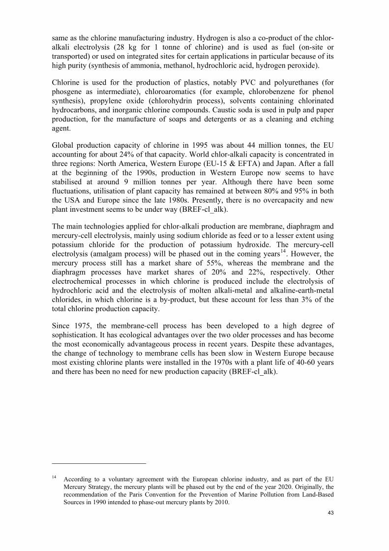
43
same as the chlorine manufacturing industry. Hydrogen is also a co-product of the chlor-alkali electrolysis (28 kg for 1 tonne of chlorine) and is used as fuel (on-site or transported) or used on integrated sites for certain applications in particular because of its high purity (synthesis of ammonia, methanol, hydrochloric acid, hydrogen peroxide).
Chlorine is used for the production of plastics, notably PVC and polyurethanes (for phosgene as intermediate), chloroaromatics (for example, chlorobenzene for phenol synthesis), propylene oxide (chlorohydrin process), solvents containing chlorinated hydrocarbons, and inorganic chlorine compounds. Caustic soda is used in pulp and paper production, for the manufacture of soaps and detergents or as a cleaning and etching agent.
Global production capacity of chlorine in 1995 was about 44 million tonnes, the EU accounting for about 24% of that capacity. World chlor-alkali capacity is concentrated in three regions: North America, Western Europe (EU-15 & EFTA) and Japan. After a fall at the beginning of the 1990s, production in Western Europe now seems to have stabilised at around 9 million tonnes per year. Although there have been some fluctuations, utilisation of plant capacity has remained at between 80% and 95% in both the USA and Europe since the late 1980s. Presently, there is no overcapacity and new plant investment seems to be under way (BREF-cl_alk).
The main technologies applied for chlor-alkali production are membrane, diaphragm and mercury-cell electrolysis, mainly using sodium chloride as feed or to a lesser extent using potassium chloride for the production of potassium hydroxide. The mercury-cell electrolysis (amalgam process) will be phased out in the coming years14. However, the mercury process still has a market share of 55%, whereas the membrane and the diaphragm processes have market shares of 20% and 22%, respectively. Other electrochemical processes in which chlorine is produced include the electrolysis of hydrochloric acid and the electrolysis of molten alkali-metal and alkaline-earth-metal chlorides, in which chlorine is a by-product, but these account for less than 3% of the total chlorine production capacity.
Since 1975, the membrane-cell process has been developed to a high degree of sophistication. It has ecological advantages over the two older processes and has become the most economically advantageous process in recent years. Despite these advantages, the change of technology to membrane cells has been slow in Western Europe because most existing chlorine plants were installed in the 1970s with a plant life of 40-60 years and there has been no need for new production capacity (BREF-cl_alk).
14 According to a voluntary agreement with the European chlorine industry, and as part of the EU
Mercury Strategy, the mercury plants will be phased out by the end of the year 2020. Originally, the recommendation of the Paris Convention for the Prevention of Marine Pollution from Land-Based Sources in 1990 intended to phase-out mercury plants by 2010.

44
Table 14: Energy and CO2 related data for the chlor-alkaline industry (DG2413) Cost forCO2 -allowance (1)
Fuel (1) (GJ/tch)
Electricity
(GJ/tch) (1)
Energy intensity (GJ/tch)(1)
CO2 intensity (tCO2/tch)(1)
Energy cost (€/tch) 1)
Price of product (€/tch) (1) Euro
(€/tch)
Percentage of energy cost (%)
Percentage of product price (%)
Membrane (2) (chlorine)
SP(7) : 20%
0.3 4.7 5.0 0.6 67.9 210 (5) 11.5 16.9 5.5
Diaphragm (2)
(chlorine)
SP(7) : 22%
1.0 5.0 6.0 0.65 76.2 210 (5) 13.0 17.1 6.2
Mercury (2) (chlorine)
SP(7) : 55%
0 5.0 6.0 0.7 84.4 210 (5) 14.3 16.9 6.8
Membrane (3) (sodium hydroxide)
SP(7) : 20%
0.3 4.1 4.4 0.5 60.2 320 (6) 10.2 16.9 3.2
Diaphragm (3)
(sodium hydroxide)
SP(7) : 22%
0.9 4.4 5.3 0.63 67.6 320 (6) 11.6 17.2 3.5
Mercury (3) (sodium hydroxide)
SP(7) : 55%
0 5.3 5.3 0.6 74.8 320 (6) 12.6 16.9 3.9
Source: Energy consumption of current installations of the European chlor-alkaline industry ((BREF-cl_alk).

45
(1) Energy consumption and CO2 emissions are assigned to the products according to their masses: By the production of 1 tonne of chlorine 1.13 tonnes of NaOH and 0.028 tonnes of hydrogen are co-produced. (2) Per tonne of chlorine. (3) Per tonne of solid sodium hydroxide. (4) Per tonne of hydrogen. (5) Prices per tonne of product (100% concentration). (6) SP: share of production in 2000 in the area of the EU-15 & EFTA (BREF-cl_alk).
The chlor-alkali process is one of the largest consumers of electrical energy. Table 14 shows the energy and CO2-related data for the three production processes mentioned above. All processes have similar energy and CO2-intensities. The lowest intensities are achieved by the membrane process at 5 GJ/tch and 0.6 tCO2/tch per tonne of chlorine produced, 4.4 GJ/tch and 0.5 tCO2/tch per tonne of sodium hydroxide produced. For all technologies the price increases corresponding to the CO2 constraint would be less than 7% for chlorine and less than 4% for sodium hydroxide.
3.10.4. Organic Basic Chemicals (DG2414)
The turnover of the sector “other organic basic chemicals” amounted to €106 billion and its value added to €26 billion in 2004. This corresponds to about 40% of the turnover and value added figures of the entire basic chemicals sector. In recent years sharp price increases of organic chemicals have been seen, with prices almost doubling from 1999 to 2006.
Energy intensities and CO2-intensities of eight basic organic chemicals which are produced in very large volumes and which are fundamental for the entire organic chemical industry are given in Table 15.
The energy intensities of the basic organic chemicals obtained from refinery processes (steam cracking, catalytic reforming, HDA) range from 10.0 GJ (benzene from HDA) over 33 GJ (ethylene) to 192 GJ (butadiene) per tonne of product. Analogously, the CO2 intensities range from 0.7 tCO2 (benzene from HDA), to 1.9 tCO2 (ethylene), to 9.8 tCO2 (butadiene) per tonne of product. The large energy and CO2-intensities of propylene and butadiene are a result of the low product yields in the naphta steam cracking process15.
The energy intensities of the “integrated”16 processes of ethylene oxide and mono ethylene glycol amount to 51.5 GJ/tch and 64.5 GJ/tch, respectively. The total CO2 intensities of the integrated production process amount to 3.7 tCO2/tch for ethylene oxide and 4.6 tCO2/tch for mono ethylene glycol.
Based on an allowance price of €20/tCO2, the CO2 allowance cost as a percentage of the product prices ranges from about 2% (benzene from HDA) to 11.5% in the case of mono ethylene glycol and 21.3% for butadiene.
15 The energy and CO2 intensities of propylene and butadiene are calculated proportionate to their
relative production yields from the total energy and CO2 intensity of "high value chemicals" from the naphta steam cracking.
16 The "integrated" intensities account for the proportionate intensities of the ethylene prodcution.

46
Table 15: Energy and CO2 related data for the production of basic organic chemicals (DG2414)
Cost for CO2 -allowance Fuel (GJ/tch)
Electricity (1)
(GJ/tch)
Energy intensity (GJ/tch)
CO2 intensity (tCO2/tch)
Energy cost (€/tch)
Price of product (€/tch)
Euro (€/tch)
Percentage of energy cost (%)
Percentage of product price (%)
Ethylene (1) 34 n/a 33 1.9 355 900 (3)
(5/2007) 38 10.7 4.2
Propylene (1)(2)
57 n/a 57 2.9 600 850 (3)
(5/2007) 58 9.7 6.8
Butadiene (1)
(2)192 n/a 192 9.8 2020 920 (3)
(5/2007) 196 9.7 21.3
Ethylene oxide (integrated) (4)
51.3 0.2 51.5 total: 3.7process related: 0.7
542 890 (3)
(5/2007) 74 13.7 8.3
Mono ethylene glycol
(integrated) (5)
64.2 0.3 64.5 4.6 678 810 (3)
(5/2007) 93 13.7 11.5
Vinyl Chloride Monomer (VCM) (integrated) (6)
20.7 3.7 24.4 1.6 247 600 (3)
(5/2007) 32 13.0 5.3
Benzene from pygas
9.5 0.9 10.4 0.8 113 870 (3)
(5/2007) 16.2 14.3 1.9
Benzene from HDA
9.7 0.3 10.0 0.7 106 870 (3)
(5/2007) 14.9 14.1 1.7
Benzene from reformate
14.4 1.4 15.8 1.2 171 970 (3)
(5/2007) 24.5 14.3 2.5
Para-Xylene from reformate
21.6 2.1 23.7 1.8 256 880 (3)
(5/2007) 36.7 14.3 4.2
Source: Energy consumption of current installations for the production of basic organic chemicals in Europe (BREF-orgchem).

47
(1) Obtained by steam cracking of naphta. (2) Calculated from energy and CO2-intensity of high value chemicals (ethylene, propylene, butadiene, hydrogen, benzene) with 17.5 GJ/thvc and 0.9 tCO2/thvc assuming a product yield of 28.4% ethylene, 16,5% propylene and 4.9% butadiene. (3) Prices according ICIS pricings for Europe in May 2007. (4) Includes energy and CO2 intensities of ethylene production (integrated). Selectivity from ethylene to ethylene oxide of 75% corresponds to process emissions of 0.7 tCO2/tEO . (5) Includes energy and CO2 intensities of precursors ethylene and ethylene oxide (integrated).Yield of mono ethylene glycol from ethylene oxide: 80% (6) Includes energy and CO2 intensities of feed materials ethylene (0.47 tEt/tVCM) and chlorine (0.6 tEt/tCL2) (integrated).
3.10.5. Polymers (DG2416)
Today industrial polymers are an essential part of everyday life and are used in virtually all end products, either a part of the final good or for packaging the actual product. Polymers are predestined for mass production processes due to their low material cost (per volume), easy processing characteristics as well as their easy and flexible shaping abilities (by extrusion, moulding, and so on). Moreover, polymers cover a wide range of different material properties making them useful for a vast number of appliances. For many applications of polymers there exist no economically viable alternatives; other applications have only been feasible at all by using polymers (such as certain membrane applications).
By definition a polymer is a macromolecule that is composed by identical or similar structural units thereby forming main and side chains. There are various types of polymers which are distinguished by their chemical composition. Production volumes of polymers vary from very large volume polymers (such as polyethylene (PE), polypropylene (PP)) for commodity applications (such as packaging) over engineering polymers (like polyamide (PA), polymethylmethacrylate (PMMA), polycarbonates (PC)) produced in large volumes for technically more advanced applications (fibres, optical products) to high performance polymers (polytetrafluorethylene (PTFE), polyetheretherketone (PEEK), polyimide (PI)) produced in relatively low volumes for special applications (examples are coatings, electronics, micro-/nanotechnology). Lower polymer production volumes usually go along with a higher degree of specification and so with higher prices and value-added. Plants for the production of large and very large volume polymers are usually near refineries which provide them with the raw materials.
The total volume of polymers produced worldwide is about 170 million tonnes (2003) from which about 50 million tonnes are produced in the EU-15. The polymer-manufacturing industry employs in the EU-15 more than 70 thousand people (BREF-polymer).
This section refers mainly to commodity polymers which are produced in (very) large quantities at relatively low costs for (very) large volume products (such as bottles, tubes, profiles). The polymers addressed in Table 16 cover about 70% of polymer production by volume in Europe.

48
Table 16: Energy and CO2 related data for the production of polymers (DG2416) Cost for CO2 -allowance Fuel
(GJ/tch)
Electricity
(GJ/tch)
Energy intensity (GJ/tch)
CO2 intensity (tCO2/tch)
Energy cost (€/tch)
Price of product (€/tch)
Euro (€/tch)
Percentage of energy cost (%)
Percentage of product price (%)
Polyethylene LDPE (integrated) (1)
SP(6): 16.5% (including LLDPE)
38.1 0.4 38.5 2.2 390 1230 (2)
(5/2007) 43.5 11.2 3.5
Polyethylene HDPE (integrated) (1)
SP(6): 11.1%
37.6 1.2 38.8 2.2 400 1260 (2)
(5/2007) 44.8 11.2 3.6
Polypropylene PP (integrated) (1)
SP(6): 16.1%
60.9 1.2 62.0 3.3 642 1190 (2)
(5/2007) 65.0 10.1 5.4
PVC suspension (integrated) (1)
SP(6) total PVC: 11.9%
23.6 4.7 8.2 1.9 279 1010 (2)
(5/2007) 37.5 13.4 3.7
PVC emulsion (integrated) (1)
SP(6) total PVC: 11.9%
28.6 5.6 14.1 2.3 320 n.a. 45.3 14.2 n.a.
Polystyrene General Purpose PS (integrated) (1)(3)
SP(6) total PS:
6.4%
17.4 0.7 18.1 1.18 187 1430 (2)
(5/2007) 23.6 12.6 1.7
Polystyrene High Impact PPS (integrated) (1)(3)(4)
SP(6) total PS:
6.4%
17.8 0.7 18.5 1.2 189 1470 (2)
(5/2007) 24.0 12.7 1.6
Polystyrene EPS
18.1 0.7 18.8 1.22 191 1600 (2)
(5/2007) 24.4 12.7 1.5

49
(integrated) (1)(3)(5)
SP(6) total PS:
6.4%
PET (TPA process) (integrated) (1)
SP(6): 7.8%
25.1 1.2 26.3 1.9 270 1400 (2)
(5/2007) 38.3 14.2 2.7
Source: Energy consumption of current installations for the production of large volume polymers in Europe (BREF-polymer).
(1) Refers to the total energy and CO2 intensities of the share of feed chemicals (see Table 15) to produce one tonne of polymer as well as the actual production process of the polymer. (2) Prices according ICIS pricings for Europe in May 2007. (3) Due to a lack of data for the styrene production process the given values refer to the energy and CO2 intensities of the feed chemicals of the styrene process (i.e. benzene and ethylene) as well as the production process of polystyrene itself. (4) HIPS: rubber additives such as polybutadiene not taken into account. (5) EPS: blowing agents (e.g. pentane, CO2) are not taken into account. (6) SP: share of production. The mentioned values refer to shares of total polymer production volume in the EU-15 & EFTA.
The energy intensities of the commodity polymers listed in Table 16 range from 8.2 GJ (PVC suspension) to 62 GJ (polypropylene) per tonne of polymer. The integrated CO2-intensities taking into account the total emissions of the polymerisation process as well as the total emissions of the feedstock materials range from 1.2 tCO2 (polystyrene) to 3.3 tCO2 (polypropylene).
Based on an allowance price of €20/tCO2 the incremental costs for the CO2 allowance range between €24 and €65 per tonne of polymer. These costs would be equivalent to price increases of about 1.5% (polystyrene) to 5.4% (polypropylene) based on energy and product prices in May 2007.
3.10.6. Refineries
The purpose of oil refineries is to convert crude oil into useable products. Usually the refinery products are classified in terms of “light” to “heavy” following the way crude oil is separated by distillation into fractions: light fractions (LPG, gasoline, naptha), middle fractions (kerosene, diesel), heavy fractions (fuel oil, lubricating oils) and residuum (wax, bitumen, tar).
Oil refineries are complex plants which comprise a combination and sequence of different processing facilities. Typically, in a refinery the outputs of a process are fed into subsequent different processes, referred back to a previous process or blended with other outputs to form marketable products.
Distillation is the primary17 and fundamental process in the processing of crude oil and is carried out in all oil refineries. Distillation processes (atmospheric distillation, vacuum distillation) sort heavier from lighter components of the crude oil according to their boiling point. What follows is a further processing of the distillation fractions in diverse 17 After pretreatment of the crude oil by desalting.

50
processes to saleable products by breaking, combining and re-shaping the containing hydrocarbons (BREF-refinery).
Pivotal conversion facilities are diverse cracking processes in which longer hydrocarbons (heavy fraction) are broken down into smaller hydrocarbon molecules (light fraction, light hydrocarbons). The basic cracking processes employed are thermal cracking (steam cracker, visbreaking, coker) and catalytic cracking (fluid catalytic cracking, hydrocracking). Steam cracking is mainly used for the generation of organic feedstock for the chemical industry such as methane, ethylene, propylene, butadiene and aromatics.
Another important refining process is catalytic cracking which converts the naphta fraction by re-shaping and breaking of the hydrocarbons. The main product of catalytic cracking is the reformate which contains mainly high-octane aliphatic and aromatic compounds. The reformate is used for blending of gasoline or for extraction of aromatics such as benzene, toluene and xylene for the chemical feedstock. Significant by-products of catalytic cracking are liquid petroleum gas (LPG) and hydrogen. The hydrogen produced is needed as feed material in several processing steps in a refinery such as hydrocracking and hydrotreatments (hydrodesulphurisation, hydrodenitrification, saturation of olefins and aromatics). Other important methods for hydrogen production in a refinery are steam reforming and partial oxidation of hydrocarbons. Steam reforming is the most commonly used process method for the hydrogen production and it is less CO2-intensive than the partial oxidation process.
Other important re-shaping and combining processes of hydrocarbons are alkylation (reaction of olefins with isobutane, to form isoparaffins with a high octane rating), polymerisation (converting propene and butene to high octane gasoline blending components), etherication (producing methyltetrabutylether (MTBE), ethyltetrabutylether (ETBE), gasoline additives from isobutylene), and isomerisation (converting paraffins and olefins to hydrocarbons with higher octane rating).
The CO2-intensity of the Europen refinery industry varies widely in a range of 0.02 tCO2 to 0.8 tCO2 per tonne of crude-oil refined. The specific emissions depend very much on the refinery complexity as more complex refineries tend to consume more energy and consequently emit more CO2. Most of the refineries show CO2 intensities in the range of 0.08 tCO2 to 0.4 tCO2 per tonne of crude oil which would correspond to allowance costs of €1.6 to €8 per tonne of crude oil at an allowance price of €20/tCO2 (BREF-refinery).
The energy consumption of European refineries ranges from 1.7 GJ to 5.4 GJ per tonne of processed crude oil. About 35-40% of the total process energy is consumed in distillation facilities (atmospheric and vacuum distillation) as the entire volume of the processed crude has to be heated to a temperature of about 350ºC. The most energy-intensive processing steps are catalytic reforming (1.4 GJ/tcrude - 2.9 GJ/tcrude), coking (0.8 GJ/tcrude - 1.2 GJ/tcrude), hydrocracking (0.6 GJ/tcrude - 1.2 GJ/tcrude), catalytic cracking (0.12 GJ/tcrude - 2.0 GJ/tcrude) as well as etherication (2 GJ - 4 GJ per tonne of MTBE) (BREF-refinery).
The refinery capacity in the EU-15 and EFTA was about 700 million tonnes of crude oil at the end of the 1990s. This volume was processed by 104 refineries of which about 10 were specialist refineries producing mainly lubricating oil or bitumen. Refineries are located mainly close to the sea or to a large river in order to facilitate the sea transport of raw materials and products. Due to large overcapacities only a few oil refineries have been built in Europe in the last 25 years (BREF-refinery).

51
3.11. Summary
Based on the above calculations for more than 50 different products and production processes in energy intensive sectors, the impact of a €20/tCO2 allowance price on output prices should be between 0.1 and 5% for most of the products considered, assuming full pass through of CO2 along the upstream supply chain. Doubling the CO2 price to €40/tCO2 and retaining the assumption of full pass through would double these figures.
In the metals sectors, the primary production of steel and aluminium would require higher price increases to recover fully the costs of a binding carbon constraint. In the case of primary steel (integrated steelworks) price increases would be in the range of 6.5% to 12%, whereas in the case of primary aluminium necessary price increases are likely to be in the range from 7.5% to 10%. In the area of building materials, full pass through of CO2 prices would correspond to price increases of more than 20%-45% in the cement and lime industries, but prices of most types of ceramics and glass would typically have to rise by no more than 2%. In the basic chemicals sector, ammonia prices could rise by up to 14% to 25% or more, depending on the production technology and fuel input used, and this would have knock-on effects on most types of fertilisers. However, price increases needed to recover the carbon constraint imposed on basic organic chemicals and polymers would not need to exceed 7%.
For most of the energy-intensive industries, cost increases are directly related to the carbon content of the fossil fuel they use (direct costs). Other sectors, such as the energy-intensive production of primary aluminium, are exposed to cost increases resulting from the pass through of higher costs of their electricity suppliers (indirect costs). Finally, production processes in some sectors, such as the production of cement and lime, also emit CO2 independent of the energy mix they use (process emissions).
Typically, production from recycled material requires only a fraction of the energy needed by production from virgin material. Thus, the price increases needed for iron and steel, aluminium, copper or even glass production based on recycled input would be much less affected by the imposition of a carbon constraint than the same products based on primary inputs. Imposing a carbon constraint would therefore make recycling more attractive.
Moreover, the upper and lower ranges given above for identical products are largely determined by alternative production processes of fuel inputs. Switching to less carbon-intensive fuels and switching to more energy-efficient production processes could already reduce the cost increase stemming from the carbon constraint by 30% to 50% or even more, for example, in the production of cement or clinker, paper and pulp production or most of the chemical products analysed.
As European climate policy is phased in gradually, so could the price increases necessary to take into account rising (opportunity) costs from the carbon constraint. Assuming a phasing in of a tighter carbon constraint by 1 percentage point annually would translate the price increases derived above into annual price increases of 0.01 to 0.5% for most of the products analysed, and to 0.5 to 1.0% for the primary production of steel and aluminium. This would be well below price increases experienced in recent years. Outliers would be the cement and lime industry and the production of ammonia (an input for fertilizers), if they continued to be produced in a very carbon-intensive way despite the availability of low-carbon alternatives, where the annual price increases needed to

52
recover the (opportunity) cost of such a carbon constraint would amount to 2 to 4%. However, these products are largely sterilized from extra-EU competition.

53
4. MEASURING EXPOSURE TO (INTERNATIONAL) COMPETITION – AND IMPLICATIONS FOR COST-PASS THROUGH POSSIBILITIES
The previous analysis has clearly shown that imposing a carbon constraint on European energy and carbon-intensive industries, branches and production processes can have significant cost implications. If producers are not able to pass these higher production costs through to their clients, or to adjust their production processes to become significantly more energy and carbon efficient, they will be forced to leave the market in the long run.
The possibility to pass through higher costs largely depends on the (in)ability of clients to change their supplier by switching to non-EU producers and/or on their substitution possibilities. The fewer alternative producers or products available to their clients, the easier it will be for producers to pass through higher costs. Such substitution possibilities are typically measured by price elasticities of demand, and in the international context, by so-called Armington elasticities that try to measure substitution possibilities between domestic and foreign supply.
If one wants to quantify the consequences of unilateral carbon constraints, it is necessary both to analyse the exposure of these industries to international competition and to look more carefully at the structure of the relevant markets and competition in general, as, for example, revealed by price elasticities and concentration indices.
However, reliable estimates of these price and Armington elasticities do not seem to exist for the markets analysed in this study (see for example annex 2 dealing with Armington elasticities). Thus, alternative indicators to measure exposure to (international) competition are needed. Therefore, an analysis of the openness of these industries to trade and market and price dynamics will be undertaken in the following three sections of this chapter before having a closer look at market concentration and other issues in section 4.4.
4.1. Openness to trade
As regards international competition and in the absence of firm data on price and Armington elasticities, openness to trade could serve as an indicator of the degree of international competitive pressure that industry branches face. The chart below (Figure 8) shows the ratio of extra-EU exports and imports to turnover of a number of energy-intensive sectors. For reasons of data availability, values for exports and imports refer to extra-EU trade for the year 2005, while the turnover figures use data from 2004.
The “cement and concrete” branch stands out as being considerably less open to trade than the other energy-intensive sectors, with exports and imports together amounting to less than 10% of turnover. Other construction-related branches (stone, glass) also appear among the relatively closed branches. At the other end of the scale, both “basic precious and non-ferrous metals” (which includes aluminium manufacture) and the branch “basic chemicals, pesticides, other agro-chemicals” are relatively open to trade.

Figure 8: Openness to extra-EU trade 2004/2005
01020
30405060
7080
Total
Man
ufactu
ring
Non-fe
rrous
meta
lsTu
bes
Basic
chem
icals
+ agro
-chem
icals
Texti
les: W
eavin
g & fin
ishing
Man-m
ade f
ibres
Texti
les: P
repara
tion &
spinn
ing
Pulp, p
aper
and p
aperb
oard
Venee
r, plyw
ood,
etc.
Ceramic
good
s and
clay
prod
ucts
Basic
iron &
stee
l, ferr
o-allo
ys
Glass a
nd gl
ass p
roduc
ts
Stone,
mineral
prod
ucts
& misc
. ...
Cemen
t, lim
e & co
ncret
e
Imports
Exports
% o
f tur
nove
r
Source: EUROSTAT Structural Business Statistics and Comext
A more disaggregated presentation of the exposure to trade of different products, based on Eurostat’s Prodcom database for 2006, is given in annex 1. It highlights the need for disaggregation and for a bottom-up analysis, as openness to trade within a well-specified industry and branch still differs significantly between individual products within such a branch or industry.
Moreover, high openness to trade does not automatically imply a bad/good international (cost) competitiveness position triggered by differences in relative prices between EU and non-EU producers. It is rather an indication of the integration of the EU economy in the world market and of the international division of labour.
Thus, instead of only comparing exposure to trade and using this as a synonym for exposure to international competition, one often also focuses on the trade balance. A longer-lasting trade surplus is taken as an indication of an underlying healthy competitiveness position while a long-lasting trade deficit is seen as a sign of a weak competitiveness position.
However, such high import or export ratios and surpluses/deficits are often triggered by long-term capacity constraints, specialisation on the supply side, or by domestic supply capacities being much higher/lower than domestic demand. Thus, the high export share for (for example) tubes in total turnover might be more the result of high demand for tubes for pipeline construction in the rest of the world, combined with the specialised technical know-how concentrated in the EU, than the result of relatively low energy, labour or capital costs in the EU. Nevertheless, longer-term trends in the trade balance might be a good indication of the comparative advantages of different economic regions of the world.
Typically it is assumed that a high exposure to international trade together with a long-lasting trade deficit is also an indication of high international competitive pressure, which makes it difficult to easily pass through unilateral cost increases. Thus, primary aluminium producers in the EU might have difficulties to pass through unilateral cost
54
increases to their clients. However, primary aluminium production and processing is also an example of a global market characterised by a global oligopoly, in which EU producers and processors have the advantage of a highly depreciated capital stock, so that the costs of capital have already largely been paid back by past production18.
4.2. Trade and regional market-share dynamics – and the role of (real effective) exchange rates
Alternatively, or as well as simply looking at the openness to trade, one could analyse market dynamics, that is, the shares of European producers in world markets, how they have developed, and how European producers were or were not able to benefit from dynamically growing markets. The less they could benefit from growing markets and the more they lost market shares, the more intense might be their exposure to international competition.
Figure 9: World trade dynamics for energy intensive sectors from 2000 to 2005
World Trade
+ 74%
+ 111%
+ 162%
+ 76%
+ 87%
+ 58%
+ 18%
+ 118%
+ 90%
50 100 150 200 250 300
28 Inorganic chemicals
29 Organic chemicals
47 Pulp of wood
48 Paper & paperboard
69 Ceramic products
70 Glass and glassware
72 Iron and steel
74 Copper
76 Aluminium
20002005
Source: UN Comtrade, HS1992 exports, ow n calculations, intra-EU27 trade excluded
Bn USD
Products of energy-intensive sectors have enjoyed extraordinarily dynamic international trade growth in recent years. Figure 9 shows that all sectors except pulp (and paper) experienced two-digit annual growth rates between 2000 and 2005, with trade in copper, organic chemicals or iron and steel growing by 15 to 20 percent annually. Similarly, cement trade (not shown in Figure 9) developed very dynamically, although starting from very low levels if compared with other energy and carbon-intensive industries.
This compares to global exports of goods expanding by about 10% annually between 2000 and 2005. The main reason for this dynamic trade and production development of energy-intensive industries can be found in the growing appetite of large developing countries like China and India, in the past characterised by a huge agricultural (and textile) sector but now turning into industrialised superpowers.
18 See section 3.3 for more detail.
55

Quite often, European producers could not fully benefit from this dynamically expanding international exchange of goods. However, Figure 10 shows that the performance has been rather heterogeneous. Some industries and branches such as glass and glassware production had a stable market share while others such as pulp and paper production, or the production and processing of paper and paperboard gained significant market share.
Figure 10: Change in extra-EU market shares for selected energy-intensive commodities, 2000-2006
0% 20% 40% 60% 80% 100%
28 Inorganic chemicals-20002006
29 Organic chemicals-20002006
47 Pulp of w ood-20002006
48 Paper & paperboard-20002006
69 Ceramics-20002006
70 Glass and glassw are-20002006
72 Iron and steel-20002006
74 Copper-20002006
76 Aluminium-20002006
7403 Refined copper, unw rought-2006
7601 Aluminium, unw rought -20002006
EU-27 Iceland Norw ay USA Canada Australia Japan Russia China India Other
Source: UN Comtrade database, HS1992
The figure also shows that it is crucial to distinguish between the production of a commodity such as copper or aluminium, and its further processing. Indeed, typically, European industry specialises in the further processing of such energy-intensive commodities, as can be seen from the much higher market share in the 2-digit Comtrade nomenclature (that typically includes production and processing) and the 4-digit Comtrade nomenclature that only covers the production of the commodity.
Competitors from other major industrialised regions such as the USA or Japan lost even more market share. This is especially surprising for the USA whose international competitiveness position did not – as opposed to that of EU companies - suffer from a significantly appreciating currency since 2001, or the imposition of a carbon constraint (as of 2005). Main winners of market share were China, Russia, India and Brazil.
Thus, other than relative cost developments seem to have dominated world market growth for these products. Indeed, it seems to be the emergence of the “BRICs” (Brazil, Russia, India and China), both on the supply and on the demand side, that has significantly altered traditional global trading patterns.
56
Beyond typical elements such as production cost components, the relative competitiveness position of companies in international markets (as opposed to domestic markets) is largely influenced by exchange rate levels and exchange rate changes. As can be seen from table 17, over recent years, the nominal effective exchange rate (NEER) of

57
the euro has substantially appreciated (+21.4%) against the basket of currencies of the main trading partners, more than recovering the losses it experienced in the 1996 to 2000 period (-14.6%). It has appreciated even further in 2007. This fluctuation had definitely a bigger impact on the relative competitiveness position than the unilateral imposition of regulatory constraints such as a carbon constraint. However, while in the earlier years the euro's depreciation facilitated life for European companies, its subsequent appreciation has definitely made it more difficult over the last years, which coincided with the imposition of a unilateral carbon constraint, and the growing role of the BRICs in international trade.
Table 17: Nominal and real effective exchange rates for the euro area, 1996 - 2006
% change over the period
1996 – 2000 2001 – 2006
NEER (1) -14.2 21.4
REER ULC (2) -25.8 17.5
REER GDP (2) -22.3 16.3 Source: Cigan/Zogala (2007) (1) NEER: nominal effective exchange rate vis-à-vis 19 trading partners, double export weighting. (2) REER: real effective exchange rate. The figures given for the REER are corrected for the relative changes of the GDP deflator or of unit labour cost (ULC), i.e. .changes in wage costs after correction for changes in labour productivity.
The real effective exchange rate, that also explicitly takes into account relative unit labour cost developments in manufacturing industries in the most important competing economies, shows a somewhat more favourable picture, albeit not for all European countries. Indeed, while the nominal effective exchange rate recovered by more than 21% in the period 2001 to 2006, after having declined by about 14% in the 1996/2000 period, the real effective exchange rate recovered by less (17.5%) than it lost in the earlier period (25.8%).
However, the impact of both the nominal and real appreciation on the export performance seems to have been rather modest. A 1% appreciation of the real effective exchange rate seems to have reduced the level of extra-euro area exports by 0.2% after one year and by about 0.25% after two years with no further significant additional impact afterwards (see Cigan/Zogala, 2007).
Assuming that a unilateral increase in production costs due to a positive carbon price imposed on EU enterprises has similar effects as an increase of the same size in unit labour costs the impact on exports should also be similar. Thus, the estimated short and long term elasticity of export demand to the estimated cost increase in the range of one to five percent over a ten-year period would trigger a decline in exports relative to the baseline of less than 1% over this period for most energy intensive industries. Primary aluminium, and iron and steel from integrated steel plants, which face a much higher cost increase would be an exception to this (for more details, see chapter 3).
A recent literature review of competitiveness impacts of the EU carbon constraint (Frontier Economics (2006)) also identified primary aluminium manufacture, followed by BOF iron and steel, as the activities most likely to be adversely affected. This also highlights the role of the pass-through of allowance prices in electricity prices in

58
influencing the competitiveness impacts of the carbon constraint, since the aluminium sector is not part of the European emission trading scheme.
Quirion & Hourcade (2003) observed that carbon-intensive sectors – with the exception of the non-ferrous metals sector – are less exposed to extra-EU competition than the industry average. They also attempted to compare the impact of the EU carbon constraint on competitiveness with exchange rate shocks. With allowances grandfathered and a CO2 allowance price of €20/tonne they found that the impact of the carbon constraint would be no more than one-fifth that of a 10% appreciation in the exchange rate of all EU currencies against all other currencies. However, their analysis was conducted at quite an aggregated level – industry was divided into 12 sectors – and did not take account of the impact of the carbon constraint on electricity prices.
4.3. Price and market developments – some evidence from the pre-carbon-constraint period
Figure 1111 shows in some detail how domestic production, domestic output prices and exports and imports developed for some energy-intensive industries in the period preceding the imposition of a carbon constraint. The period was characterised by rather sluggish growth in the EU, a significant appreciation of the euro and of the currencies pegged to it, and energy prices initially retreating from their peak experienced in 2000 before embarking in early 2002 on an upward path, eventually leading to record nominal levels in 2006/2007. The period also includes the terror attacks of 9 September 2001 and the war in Iraq starting in early 2003.
Of the 17 branches, nine suffered a – sometimes even very significant – production loss, the output of glass remained rather stable (-0.2% over five years), while seven branches enjoyed more or less dynamic output growth. However, an output loss did not necessarily reflect a deterioration in international competitiveness. Indeed, three of the seven branches in which production fell, and for which trade data were available (preparation of textiles, man-made fibres and basic precious and non-ferrous metals), experienced declining imports and rising exports during this period, not necessarily a combination characterising a loss in international competitiveness. In addition, 10 of the 15 branches for which trade data were available showed an improvement in their trade balance while five experienced a certain modest erosion, the balance itself remaining in surplus. Of the latter, the cement, lime and plaster industry suffered the most pronounced decline in its trade balance, its trade surplus deteriorating from about 6% of annual turnover to 2.3%.
In addition, the correlation between price and production or trade developments is less straight forward than one would expect, or sometimes even “counter-intuitive”. Indeed, while it is true that (including glass) 10 of the 16 branches in which domestic prices increased also experienced a decline in domestic production, five benefited from both rising domestic prices and rising domestic production. In fact, plotting price changes against production changes shows a positive correlation, suggesting that at times of buoyant economic and sector-specific growth it is much easier to pass through cost increases and to increase prices than at times of sluggish overall demand. One might want to interpret trade and price data in the same vein: the fact that 11 of the 14 branches that managed a sustained price increase also had a rising trade surplus should be seen more against the background of dynamic (global) demand growth than as evidence for growing international competitiveness.

Figure 11: Output and price changes as well as dynamics for selected European energy-intensive industries, 2000 to 2004
59
12.2
11.4
8.4
6.7
80.5
14.2
54.7
6.1
4.7
30.8
6.8
21.6
5.7
4.4
7.7
30.7
14.7
22.6
9.0
17.0
81.7
73.0
12.4
5.7
15.0
30.9
4.8
5.6
5.5
17.7
-40 -30 -20 -10 0 10 20 30 40 50 60 70
Preparation of textiles
Man-made fibres
Finishing of textiles
Ceramics not for construction
Ornamental and building stone
Ceramic tiles and flags
Basic precious and non-ferrous metals
Builders' carpentry and joinery
Bricks, tiles and construction products
Glasses
Casting of metals
Basic iron and steel
Other non-metallic mineral products
Cement, lime and plaster
Pulp & paper
Basic chemicals
Manufacture of tubes
DB1
71D
G24
7D
B173
DI2
62D
I267
DI2
63D
J274
DD
203
DI2
64D
I261
DJ2
75D
J271
DI2
68D
I265
DE2
11D
G24
1D
J272
DomesticproductionImports
Exports
Productionprice
Change over the period2000-2004, %
reducedproduction
increasedproduction
Source: EUROSTAT Comext and UN Comtrade
Overall, it seems plausible to assume that at least in the short to medium term, that is, up to a period of three to five years, demand and supply dynamics are more relevant for price setting and production behaviour than underlying cost-competitiveness considerations. Moreover, the multitude of sector and branch-specific characteristics, and developments outside the control of branch-specific decision makers, such as exchange rate or energy-price volatility, or political risks, seem to be much more important for the relative performance of sectors in the shorter run than the fine-tuning of the production-

60
cost function. In addition, the emergence and industrialisation over the last decade of economically very important key players on the global scene, such as the BRICs, had a major impact on the absolute and relative economic performance of the incumbents from other industrialised regions, including Europe.
Thus, as long as the global economy and demand for products from energy- and carbon-intensive industries continues to grow dynamically, concerns of limited pass-through possibilities of relatively modest but unilateral cost increases seem to be less well founded. However, this picture can be expected to change once this dynamic demand growth tapers off. Then, for example, in a long-lasting global recession, small cost differences and the existence or non-existence of “deep pockets” might play a decisive role in determining whether an industry or production location will survive. This would hold even in highly concentrated markets where companies are not necessarily competing against each other but where competition is between different production facilities of and the same company in different locations.
4.4. Barriers to competition in energy-intensive industries
Exposure to international competition as measured by openness to trade and the gain or loss in market share at the global level is only one facet, but an important one, for analysing the pass-through potential of industries. Another, equally important issue, is the degree of competition on a given market, indicated for example by the degree of concentration, barriers to entry and exit, or the degree of collusion between competitors on a market. Here it is typically assumed that higher degrees of concentration, of collusion or important entry and exit barriers might be harmful for competition and thus would facilitate the pass-through of (asymmetric) cost increases, while the absence of these features is typically assumed to intensify competition and, consequently, make the passing through of such cost increases more difficult.
Energy-intensive industries are typically rather capital intensive and, thus, invite for concentration to better exploit economies of scale. Figure 12, depicting a small selection of energy-intensive industries – clearly confirms this picture. The market shares of the five biggest producers on these markets range from almost 30 percent to well above 75 percent, with the markets for the basic inputs of a refined commodity (such as iron ore, or alumina production) being typically even more concentrated than the markets for the production of the refined product (different steel products or aluminium production).

Figure 12: Concentration in selected energy intensive industries – market shares of 5 biggest producers (2006)
0
1020
3040
5060
7080
90
Iron ore Nickel Alumina Copper Aluminium Zinc
%
Source: European Aluminium Association, Brook Hunt, Macquarie
In the economic literature19, four categories of indicators are typically used to measure competition. They relate to (i) market structure as (for example) reflected in concentration indices or entry and exit barriers and (dis)economies of scale and scope, (ii) supplier behaviour such as collusion, cartels or predatory pricing, (iii) consumer behaviour as (for example) reflected in the price elasticity of demand, and (iv) consumer benefits. The most common forms of weak competition materialise in formal or informal collusion, or horizontal agreements, or in the abuse of a dominant position. Motta (2004) identifies structural factors related to technology and market structure, a high degree of price and market transparency, and factors related to pricing rules and contracts as those features that facilitate collusion and the forming of some kind of cartels or agreements amongst competitors. Similar factors prima facie working as forceful barriers to effective competition are also highlighted by the Office of Fair Trading (OFT) (2005).
In 2007, London Economics (2007) in association with ZEW and RPA tried to identify industrial sectors with weak competition. Not surprisingly (given the analysis of chapter 3), the energy-intensive industries that have been analysed above feature prominently in this analysis. Indicators such as concentration indices, market entry and exit rates or capital-intensity requirements indicate the presence of market structures that are not very conducive to effective competition. For some sectors, such as the cement and lime industry, this has been confirmed by an above-average number of cartel and anti-trust cases pursued by the EU or its Member States, although the absence of such cases does not automatically serve as a proof for the absence of such behaviour.
In principle, the study has been undertaken at too aggregate a level to be taken as firm evidence of weak competition on these markets. However, the structural features identified for these industries do not seem to be very conducive to strong competition. This suggests that the barriers to competition identified could be sufficient to enable the pass through to downstream industries of a non-trivial part of higher production costs.
19 For a recent overview of the relevant literature see for example Lee (2004).
61

62
5. POTENTIAL BRANCH-LEVEL AND WIDER ECONOMIC IMPACTS, AND THE RISK OF CARBON LEAKAGE
5.1. Profitability, carbon leakage and the value chain
Enterprises exposed to a carbon constraint either themselves, or through their upstream suppliers who pass through their higher (opportunity) costs, typically face higher production costs. If these tried to pass through to their clients these higher costs, in a world of perfect competition they would immediately be crowded out of the market if their competitors producing perfect substitutes were not confronted with an identical cost increase (unless flexible exchange rates corrected for this).
In a world of imperfect competition and rather sticky exchange rates, these enterprises can either try to pass these higher costs through to their clients and suffer a certain decline in demand with profits remaining relatively unchanged, or they may try to first shoulder these higher costs through a (temporary) squeeze in their mark up. In this case, part of their higher costs will effectively be born by taxpayers as the tax bill would be reduced correspondingly. In the medium term, they might also try to improve their “x-efficiency” by reducing slack, innovating, and – of course - improving their energy and carbon efficiency. In any case, as a tighter carbon constraint would be phased in over a longer period, for example through tightening by 1 percentage point annually, it might also be possible to phase in the cost increase and the necessary price increase over a longer period.
Given the importance of electricity in overall energy costs (particularly for a branch such as primary aluminium production), reducing electricity costs is obviously key to maintaining the competitiveness of energy-intensive industries in general, and especially the (primary) aluminium industry. There are essentially just two ways to do this: lowering electricity prices, for example through increased competition and efficiency in electricity production, and/or by increasing the energy efficiency of energy-intensive industries themselves.
The introduction of an emissions constraint through the carbon constraint places a value on emission (allowances) that should be included as a production cost. If EU ETS emission allowances are given out for free, then the ability of electricity producers to pass through the opportunity cost of allowances in prices allows them to earn an economic rent. The same should hold true for energy-intensive industries themselves, as they should also aim to pass through to their clients the higher opportunity costs of the carbon constraint.
An aluminium producer that responds to this situation by building or acquiring its own power plant and, for example, receiving free of charge a corresponding amount of emission allowances captures part of this rent. If the producer values this electricity in its internal accounting at the price it paid prior to the introduction of the carbon constraint (that is, excluding the cost of emissions), then its financial profits will be unchanged from the situation before the introduction of the emission trading scheme, when it bought its electricity from outside.
However, this numerical stability in the financial value of profits masks the fact that the source of the profits has changed. Prior to the introduction of the carbon constraint the firm made a profit by selling aluminium at a price greater than its production costs. After the introduction of the carbon constraint and deciding to produce its own electricity, the

63
firm makes a profit by subsidising its aluminium production through not including the value of emission allowances in the cost of the electricity it produces. The new, vertically integrated firm would then in effect consist of a power generator that supplies electricity at below market prices to an aluminium plant that would otherwise be less profitable. The vertically-integrated firm could earn the same profits by selling its electricity on the market.
The crucial distinction is between profitability and competitiveness: profitability in this example is positively affected due to the “windfall” of free allocation of allowances. Competitiveness, however, depends on the impact on marginal production costs of the price of emission allowances (see Frontier Economics (2006), McKinsey/Ecofys (2006)). Thus, while at first glance it might make a difference for the competitiveness position of industries whether they have to pay for allowances of whether they get them allocated for free, at second glance it becomes clear that free allocation would have a positive impact on profits only, while the competitiveness position would not change due to the increased (opportunity) costs of being obliged to surrender the allowances (McKinsey/Ecofys (2006)).
Nevertheless, in the longer run and in a world of fierce competition, a permanent squeeze in profit margins could affect the overall competitiveness position and investment decisions:
• The competitiveness position could be affected notably in crisis situations where production costs could no longer be recovered over a longer period: then having a “deeper pocket” than major competitors would force the latter to leave the market earlier, potentially improving the possibility for the survivor with the deeper pockets to increase prices afterwards.
• Investment decisions might be affected as investment capital might always be looking for the highest rate of return, after correction for risks. Thus, reduced profit margins in a world of selling instead of giving away allowances might trigger relocation decisions to locations neither imposing now nor expected to impose a carbon constraint in the longer run, but being otherwise (closeness to markets, infrastructure, rule of law, provision of public goods, taxation and so on) as attractive as the present location. However, to really influence investment behaviour the differences in profit margins must not be negligible, as relocation activities themselves typically come at a rather high price.
An increase in an EU industry’s production costs may reduce both domestic and extra-EU demand for its output, depending on the EU industry’s price-setting ability and the elasticity of non-EU supply. If the carbon constraint results in EU production being replaced by non-EU production, “carbon leakage” will occur. This is more likely the less EU producers themselves influence world market prices, the more difficult it is for downstream industries (such as aircraft industries or car manufacturers) to adjust their production so as to reduce their use of the output of energy-intensive industries (such as steel or aluminium), and the easier it is for these non-integrated downstream industries to switch suppliers.
In the short run, delocalisation activities would probably not take the form of closing production plants in Europe and opening new ones (to serve the European market) in non-EU locations. Rather it would take the form of not expanding production capacities

64
in case of growing markets, and of downscaling or giving less priority to (maintenance) investment in EU locations.
On the other hand, the decline in demand for a certain production process, such as primary aluminium or iron and steel produced in integrated steelworks, might also result from them losing market share to competing intra-EU suppliers that do not produce virgin material, but recycle scrap, such as producers of secondary aluminium, or steel production through the electric arc furnace process. Indeed, as recycling is typically much less energy intensive than virgin production, imposing a carbon constraint should work in favour of recycling, partly mitigating the carbon leakage problem.
Typically, energy-intensive industries figure high up the value chain, and they provide critical input for numerous economic activities. Thus, rising production costs at this level will also lead to rising production costs along the value chain, unless fierce competition in energy-intensive industries makes passing through these higher production costs impossible, even in the longer run. In this latter case, the economic implications of the carbon constraint would remain limited to energy-intensive industries.
In all other cases, the additional production costs resulting from the carbon constraint will trickle down the supply chain. For example, rising cement prices will trigger higher costs for the construction sector, and higher steel and aluminium prices will trigger higher production costs for car manufacturers or shipbuilding. The more cost increases are passed through to downstream industries the better it will be for the profitability of upstream industries.
Some industries may face a double cost increase, such as the fertiliser industry: first it might suffer from the higher costs of the production of ammonia, a crucial input for the production of most fertilisers. Then it may suffer from the carbon constraint imposed on its own process emissions. These indirect and direct cost increases and their magnitudes have been analysed in chapter 3.
Once again, downstream enterprises exposed to such price increases have different options for responding to this challenge. They can try themselves to pass through these higher production costs, they might accept a (temporary) squeeze in their profit margins, or they may invest in adjustment efforts to reduce their reliance on the input that has become more expensive and/or invest in other cost-reducing activities. In any case, given the downstream character of their activities, the cost increase these downstream industries face should only be a fraction of the cost increase faced by the upstream industries.20 Thus, the impact on production costs and, thereby, on the international competitiveness position of these industries should remain rather limited.
Nevertheless, for some downstream industries it might be worthwhile to invest in alternative technologies: aircraft producers might try improve the design of their aircraft to save on aluminium input, while car manufacturers might do the same to save on steel. Such abatement efforts are the more likely the more such innovation would also generate benefits for end users, for example by improving the fuel efficiency of aircraft and passenger cars.
20 A 10% price increase of an input that accounts for 10% of all inputs would trigger a cost increase for
this downstream industry of only one percentage point.

65
In any case, one should avoid the trap of double counting along the value chain, that is, if production cost increases in upstream industries due to a carbon constraint are passed through to their clients, they should be counted as a burden for the downstream industries only. Ideally, in the longer-term the end-user should shoulder all the burden – and adjust its demand by favouring less carbon-intensive products. This is, after all, the main purpose of imposing a positive carbon price.
5.2. Quantified ex-ante estimations of economic effects
Numerous studies have been produced to analyse the potential effect of imposing a carbon constraint on energy-intensive European industries. There is little controversy about the mechanisms at play in such a case. These include costs, influence on international competition or the risk of carbon leakage or delocalisation, as described above. However, significant differences between these studies can emerge when it comes to quantifying the importance of the different mechanisms and effects.
Typically, one can distinguish between bottom-up and top-down approaches. The first analyse at a rather disaggregated level the impacts of imposing a carbon constraint on individual or several sectors. These bottom-up approaches are normally not based on economic models but are based on sector-specific evidence, the latter itself either being derived from empirical evidence or from expert interviews or some other form of then typically difficult-to-verify other sources. In contrast to this, there also exist top-down approaches that are typically based on general or partial equilibrium economic models. These top-down approaches often transpose findings having shown some value added at the aggregate level and in some specific regions of the world (such as the USA) to a specific question under investigation.
This section 5.2 tries to summarise and analyse the findings of some of these studies, including two model-based bottom-up studies.
5.2.1. Model-based ex-ante estimations
Model-based estimations of the economic impacts of imposing a carbon constraint on the EU economy mostly consider ex-ante evidence only. This evidence is obtained from policy simulations using either top-down or bottom-up economic models. Top-down models (Computable General Equilibrium (CGE) or macro-econometric models) simulate the economy-wide effects of a selected policy measure taking into account interaction and spillover effects across the economy. Hence, the impact of a policy on a specific sector (for example, energy-intensive industry) also accounts for the effects on all other sectors and possible substitution effects between them. The drawback of top-down models is their fairly aggregate structure, which does not allow very detailed sectoral presentation of the results. However, frequently these top-down approaches do not catch important features of the industries to which they are applied, such as imperfect competition, market-entry and exit barriers of economies of scale and/or of scope. Unfortunately, all these features are characteristic for the energy-intensive industries analysed here.
Bottom-up models are partial equilibrium models, which only represent one specific economic sector (for example, cement or steel). They often incorporate detailed information about production technologies, cost structure and abatement options concerning the sector. Changes in supply and demand conditions at the world level determine the outcome of the policy measure. Since bottom-up models are usually able to deal with a wide range of technological opportunities for abatement, the costs of climate

66
policy tend to be lower than in top-down models, in which the scope of technological improvement is more limited21. On the other hand, bottom-up models may also overstate the loss of competitiveness compared with top-down approaches, since climate policy (such as a CO2 tax) affects only the modelled sector, which faces an increase of production costs relative to the other sectors, the products of which may be close substitutes for those of the modelled sector.
Climate policies are commonly modelled by assuming that countries or regions face a binding CO2 emission reduction constraint and apply an emissions trading scheme, in which case the carbon price/permit price/marginal abatement cost is endogenously given by the model. An alternative approach is to assume that a uniform CO2 tax is imposed on all sectors and countries of a region, in which case the amount of emission reduction is an endogenous outcome of the model. This case is equivalent to an emissions trading scheme covering all economic sectors with 100% auctioning of allowances.
5.2.2. GEM-E3 study22
The GEM-E3 model (European version) covers 22 EU Member States (excluding Bulgaria, Cyprus, Luxembourg, Malta and Romania) and used the Eurostat database (base year 1995). It treats separately each EU Member State and links them through endogenous trade of goods and services. The rest of the world (RoW) is exogenous in the model. The trade flows between the EU and the RoW are modelled by assuming that exports from the RoW are supplied at a fixed price, while imports demanded by the RoW depend on the price offered by the EU exporters.
The model incorporates 18 productive sectors, of which 8 are manufacturing, 4 energy products (oil, coal, natural gas and electricity) and the rest includes other economic activities (agriculture, transport, services). Of these sectors the following are here considered as energy-intensive: ferrous and non-ferrous metals, chemical products, other energy-intensive and transport. “Other energy-intensive” is a composite sector and includes non-metallic mineral products, metal products except machinery and transport equipment, and paper and printing products.
An analysis of impacts of possible post-2012 climate policy was carried out, assuming that EU countries reach their Kyoto target. From 2012 onwards no (additional) quantitative emission reduction target is imposed, but instead it was assumed that an EU-wide CO2 tax would be imposed in all sectors. The level of tax gradually increases from €19/tonne CO2 to either €25 or €45/tonnne CO2 in 2030. This is equivalent to an emissions trading scheme with 100% auctioning of allowances and covering all economic sectors. Tax (or auction) revenues are recycled in the form of reductions in employers' social security contributions. The current EU minimum tax rates on energy products, or current national tax rates, if higher, are assumed to continue to apply.
Table 18 displays the impacts of the two climate policy scenarios, depending on the level of the CO2 tax in 2030 at the EU-22 average level. All the results are expressed as a percentage difference with respect to the baseline. Note that as the study from which
21 See Capros et al. (1999): Climate Technology Strategies 2. The Macro-Economic Cost and Benefit of
Reducing Greenhouse Gas Emissions in the European Union. (ZEW Economic Studies 4). 22 Nikos Kouvaritakis, Leonidas Paroussos, Tams Revesz, Erno Zalai, Denise van Regemorter: Impacts
of energy taxation in the enlarged European Union, evaluation with GEM-E3 Europe. Study for the European Commission, DG TAXUD, 2005.

67
these scenarios are taken pre-dates the EU’s adoption of a target of a 20% cut in greenhouse gas emissions by 2020 compared to 1990 levels, the results are not necessarily consistent with this target. Nevertheless, they give an indication of how different sectors are likely to be affected by increasingly ambitious medium- and longer-term climate policies.
The falls in output in the energy-intensive sectors are several times larger than the fall in GDP. In the sector worst affected – ferrous and non-ferrous metals – the loss in output relative to baseline is roughly equivalent to one year’s growth in output, that is, the output level expected in the business-as-usual scenario for the year 2030 would be reached only in 2031 as a result of imposing the carbon constraint. The energy-intensive sectors also lose export market shares more strongly than does EU industry as a whole. The sectors covered by the ETS are somewhat more affected than those currently outside it (chemicals, transport). Revenue recycling through cuts in employers’ social security contributions benefits some of the service sectors, which are able to increase their output volumes and market shares (not shown in Table 18). Alternative approaches to revenue recycling might help to mitigate the adverse impact on the international competitiveness of energy intensive industries, but would likely have a less favourable overall economic outcome.
Table 18: GEM-E3 results of climate policy scenarios to 2030, EU-22.
case of CO2 tax 25€/t,in %-difference
case of CO2 tax 45€/t, in %-difference
GDP -0.13 -0.24 Employment 0.46 0.73 Economic welfare -0.07 -0.14 Total welfare 0.27 0.32 Exports to ROW -0.71 -1.18 Imports from ROW -0.32 -0.42 CO2 emissions -19.54 -27.21 Output volumes: Energy -5.72 -8.81 Ferrous + non-ferrous -1.34 -2.14 Chemical -0.64 -1.07 Other EI -0.78 -1.28 Transport -0.91 -1.55 Export volumes: Energy -5.52 -8.67 Ferrous + non-ferrous -2.46 -3.93 Chemical -0.94 -1.57 Other EI -1.30 -2.14 Transport -1.84 -3.12
Source: Kouvaritakis et al (2005).
The results of policy simulations are always dependent on the model specification. In the case of the GEM-E3 model a particularly sensitive assumption concerns foreign trade23. As already stated, the Rest of the World is assumed to export to the EU at a fixed price and thus EU import prices remain unchanged even if import volumes change. On the other hand, export prices increase because of the higher costs of energy, which leads to
23 See Capros et al. (1999).

68
the fall of export volumes, but less in relative terms than the prices increase (the price elasticity of EU export demand is less than -1). Hence, the improvement of the terms of trade for the EU, leading to an increase in the money inflow from exports, partly compensates the negative effect of competitiveness loss due to climate policies. According to Capros et al. (1999) the positive terms of trade effect is essential for the “double dividend” (positive employment effect) in GEM-E3 simulations24.
Technological progress is exogenous in GEM-E3, which implies that substitution possibilities induced by the CO2 price, from carbon-intensive to less carbon-intensive technologies are not incorporated. This implies that the costs of climate policies for energy-intensive industries, and thus also negative effects on competitiveness, may be overstated to some extent.
Finally, because the Rest of the World is exogenous in GEM-E3, the impact of climate policies on carbon leakage is not modelled.
5.2.2.a. COWI study for UNICE using GTAP-ECAP25
This study used a CGE-model of the world economy (GTAP-ECAP) with the usual properties (perfect competition, constant returns to scale, full employment). It reports the impacts of EU climate policies on EU exports and imports (separately for ETS sectors), which are indicators for competitiveness effects. It also provides information on carbon leakage rates. The carbon leakage rate in Table 19 is measured as the ratio of percentage- increase of emissions in non-abating countries (leakage) to the percentage reduction of emissions in abating countries.
Climate policy is modelled by imposing a cap on CO2 emissions necessary to reach the EU Kyoto target in 2010. An EU-wide emissions trading scheme is implemented in such a way, that the split of emission reduction efforts between trading and non-trading sectors is cost-effective, that is, marginal abatement cost are equalized across ETS and NTS-sectors. A limited amount of JI/CDM credits is allowed in the EU market.
Two different assumptions regarding technological developments are used: long-term adaptation and sluggish shorter-term adaptation. In the first case the allowance price resulting from EU climate policy is estimated at €17/tCO2 and in the second case at €26.5/tCO2.
The changes in EU GDP, foreign trade and carbon leakage rates in these two cases are given in Table 19 below. Compared with the GEM-E3 simulations, the COWI model gives somewhat higher macroeconomic costs, measured by the GDP change. This may to a large extent be due to the absence of revenue recycling in the COWI model, that is, the money that the regulated industries have to pay for acquiring emission allowances disappears into a “black hole”. In contrast, in GEM-E3 the recycling of this money counteracted the negative effect of higher energy costs on output and export volumes.
24 Sensitivity analyses carried out in Capros et al. (1999).do not imply, however, that the modification of
foreign trade assumptions would essentially change the conclusions regarding welfare and employment effects of the standard version of GEM-E3 model.
25 Competitiveness and EU Climate Change Policy. Interim Report produced by COWI for UNICE, October 2004.

69
Exports from the ETS sectors are also more strongly negatively affected in the COWI model, while imports of ETS sectors increase relative to the baseline. The latter implies that energy-intensive industries lose some of their market share within the EU market and that the production activities are partly relocated outside the EU, as evidenced by the reported carbon leakage rates. The GTAP-ECAP model uses much higher Armington elasticities (the elasticity of substitution between imported and domestic goods) than the GEM-E3 model26. Higher elasticities imply, in principle, more substitution possibilities between domestic production and imports and could explain the relatively strong increase of imports in the COWI model. On the other hand, increased substitution possibilities should also lead to lower increases in domestic prices and so in export prices, which should mitigate the fall of export volumes. This does not seem to be the case in the COWI model27.
Table 19: The impacts of EU climate policy in the COWI study
Long-term technological adaptation
Sluggish technological adaptation
Allowance price €17/tonne CO2 €26.5/tonne of CO2EU-25 GDP -0.36% -0.48% Total EU-25 exports -0.41 -0.55 EU-25 export to ROW > -0.5% > -1.0% Export of ETS sectors -3.8% -5.1% Total EU-25 imports -0.6% -0.9% Imports from ROW -0.4% -0.5% Imports of ETS sectors 4.3% 3.1% Carbon leakage rate 17.8% 21% Carbon leakage rate: EI-sectors
19.5%
Carbon leakage rate: other manufacturing
10.1%
Source: COWI (2004)
5.2.2.b. CPB study using WorldScan28
The focus of the study of the Netherlands Bureau for Economic Policy Analysis (Centraal Planbureau – CPB) is the macroeconomic consequences of a 30% emission reduction target in 2020, under different assumptions regarding the participation of the countries of the world in the global emission cap and trading. Two different growth scenarios are considered:
– a strong growth case (national income grows at 2.8% per annum (p.a.) in 2000-2020, emissions at 1.9% p.a. for EU-25)
– moderate growth case (national income growth rate 1.9% p.a., emissions growth rate 0.7% p.a.).
26 In GEM-E3 substitution elasticities between imports and domestic production are the following: 0.6
for energy sectors, 1.5 for industrial sectors, 0.6 for service sectors, 1.2 for agriculture and transport. In the COWI study the Armington elasticity is 4.
27 See, Capros & al (1999). Sensitivity analysis with respect to Armington elasticities indicates, however, that they have a rather marginal effect on macroeconomic aggregates in GEM-E3 model. See Koschel et al. (1998).
28 Bollen, J, Manders, T., Veenedaal, P..: "How much does a 30% emission reduction cost? Macroeconomic effects of post-Kyoto climate policy in 2020", CPB Document 64, (2004).

70
The benchmark policy case is that of strong growth combined with global participation in emissions trading (the coalition of Kyoto countries is joined by all other countries in 2010). Countries in Annex I of the UNFCCC are assumed to fulfil their Kyoto commitment in 2010 and receive emission rights on that basis in 2010. The other countries joining the coalition receive emission rights equal to their 2010 levels. The emission rights are adjusted in 2024 in such a way that all countries have equal rights per capita, the total amount of which does not exceed the global emission ceiling.
Other scenarios differ from the benchmark either by assuming different global growth rates or a lower number of participants in the global emissions trading. A Kyoto scenario is also simulated, which assumes that all the Annex I countries (apart from USA and Australia) will implement the Kyoto Protocol. The results of the scenarios for EU-25 are described in Table 20.
In these scenarios a much higher emission reduction level is reached than in the post-Kyoto scenarios of the GEM-E3 study, although the allowance price is lower than the GEM-E3 carbon tax. In the COWI study the allowance price is at the same level as in the high growth benchmark scenario of the CPB study, but the emission reduction is only sufficient to reach the EU Kyoto target in 2010. These differences mainly illustrate the cost-effectiveness of global emissions trading, which offers greater opportunities for lower-cost emission reductions.
Table 20: The impacts of climate policy in 2020 in EU-25 according to the CPB study
Benchmark Low growth, global trading
Low growth, no participation of Asia and Africa
High growth, only Annex I participation
Kyoto scenario, effect in 2010
Allowance price, €/tonne of CO2
17 4 58 129 11
CO2 emissions compared to 1990 level, %
-30 -27 -30 -30 -6
CO2 emissions compared to the baseline, %
-53 -36 -53 -53 -24
National income, % change from baseline
-0.6 -0.1 -1.8 -3.1 -0.3
Production EI, trade and transport, %-change from baseline
0 0 -4 -12 -2
Source: Bollen et al (2004).
Although not shown in Table 20, in the scenarios with global trading there are no adverse competitiveness impacts for the energy-intensive industries in Europe, as there is no asymmetric cost shock for EU producers. In the Kyoto scenarios the output losses are of similar magnitude as in the GEM-E3 Kyoto scenarios.

71
5.2.2.c. OECD study on the steel industry using SIM29
Climate policy in this study consists of setting a carbon tax on the steel industry (and the power sector) at the rate of US$25/tonne of CO2. In the benchmark scenario the tax is implemented in the whole OECD area. The impact is simulated with a numerical partial equilibrium model of the world steel industry (SIM)30.
Even compared with the GEM-E3 simulation reported above with a carbon tax of €45/tonne of CO2, this model estimates much greater reductions of output, particularly when the tax is imposed only in the EU. In EU13 (EU15 without Finland and Sweden) total steel production would fall by over 10%, and while CO2 emissions within the EU13 would fall by more than twice this (reflecting significant reductions in carbon intensity), the fall in emissions would be less than 2% at the world level, implying a strong rate of carbon leakage.
These differences could have several explanations related to modelling methodologies. The obvious one is the Armington elasticity of 8 assumed in the OECD study (for Armington elasticities in GEM-E3 see footnote 26). Such a high elasticity implies that there are ample opportunities to substitute steel produced in one region of the world for steel produced in another region and could explain large changes of output volumes. This might be justified if steel can be regarded as a relatively homogenous product across the world, where transport costs and the exploitation of economies of scope through vertically-integrated value chains do not matter: The sector “ferrous and non-ferrous metals” in GEM-E3 is much broader and consists of different kinds of products. However, an elasticity of 8, implying that an increase (decrease) in European producer prices by one percentage point would lead to a fall (increase) in demand for European steel by eight percentage points, does not seem to be matched by empirical evidence.
Another explanation may be that in the OECD study the tax is imposed only on the steel and power sectors, and the changes of output volumes are determined only by price and Armington elasticities. In GEM-E3 there are also substitution opportunities between different products, which may mitigate output changes when the carbon tax is imposed broadly across all the economic sectors.
Finally, the revenue recycling assumption (reduction in labour taxes) and the consequent decrease in labour costs in the GEM-E3 simulations may, to some extent, mitigate competitiveness losses in energy intensive industries.
5.2.2.d. OECD study on the cement sector31
As for the steel industry, a numerical partial equilibrium model (originally developed by the Commission’s Institute for Prospective Technological Studies (IPTS)) was used to simulate the impact of climate policies on the cement sector. The CO2 tax was set at a level of €15/tonne of CO2. Rather than using an Armington elasticity, in which one
29 Environmental policy in the steel industry: using economic instruments.
COM/ENV/EPOC/DAFFE/CFA(2002)68/REV1. (2003). 30 The model is developed at the Institute for Research in Economics and Business Administration,
Norway. 31 The competitiveness impact of CO2 emission reduction in the cement sector.
COM/ENV/EPOC/CTPA/CFA(2004)68/final. (2004).

72
parameter is used to capture the various “rigidities” affecting international trade, the model incorporates transportation costs, capacity utilization rates and profits for every producing country, and the average cement price for every consuming country.
In this simulation, the fall in production is relatively modest in Europe, at less than 1% below baseline in 2020. This is comparable to the results of the GEM-E3 simulations (in which cement is included in “other energy intensive industries”). Starting at very low levels, exports fall by about 0.5%, and imports rise by about 4% compared to the 2020 baseline.
As in the steel study, the fall of CO2 emissions is nearly double the fall of output as the CO2 tax induces changes in production processes (reduction of the clinker content of cement) and a switch to low-carbon fuels.
5.2.3. Ad-hoc bottom-up studies
Ad-hoc bottom-up studies have tried to collect and quantify the facts, such as major characteristics of regulated industries and the cost increases triggered by the carbon constraint. Subsequently they describe the mechanisms at play and introduce and quantify certain key assumptions, for example, the degree of competitive pressure or the possibility to pass through higher production costs to clients to be able to analyse or even quantify the effect on production, profits or carbon leakage of introducing the carbon constraint. They also consider mitigating effects, or try to take into account likely dynamic structural adjustment that would occur in the absence of a unilateral carbon constraint.
One of the more recent efforts to estimate ex-ante the effects of introducing the carbon constraint through the EU ETS on the competitiveness of selected industries without reverting to aggregate model simulations or sectoral partial equilibrium models was conducted by McKinsey and Ecofys (McKinsey/Ecofys (2006)). This study tries to quantify the effects of a carbon constraint with a price of €20/tCO2 on the international competitiveness of the steel industry, pulp and paper production, the cement industry, refining activities and aluminium production.
While it stops short of quantifying the effects of the assumed carbon constraint on output, employment, investment and profits of these industries, the study tries to quantify the cost implications of a CO2 price of €20/t CO2, and is rather explicit in quantifying the tightness of international competition by estimating the possibilities of these industries to pass through the resulting cost increase to their clients without being crowded out of the market.
McKinsey and Ecofys give the following pass-through capabilities by sector:
• Power sector: 100% pass-through capability • Steel: BOF can pass through 6% and EAF 66% of the cost increase • Aluminium: 0% pass-through capability • Cement from dry process: 0 to 15% pass-through capability • Refining: 25 to 75% pass-through capability.
However, no indication is given that these pass-through capabilities by sector are based on empirical evidence. Actually, the assumptions of rather limited pass-through capability seem to be somewhat in contradiction with historic evidence. Indeed, most of these industries have significantly increased their output prices over the last years, and all

have experienced a continued increase in outputs and rising profits, despite permanently rising production costs (higher raw material prices, higher labour costs) and – over recent years - an appreciating currency. Nor is it made clear what would happen if regulated industries would go beyond the pass-through thresholds defined by McKinsey/Ecofys, that is, the assumed price elasticities of demand are not stated.
The cost/price increases presented by McKinsey/Ecofys also look rather high compared to the estimates in chapter 3 of this study: while section three arrives at increases of (for example) 7.3% for BOF steel or 23% for the cement industry (dry process), the respective figures quoted in McKinsey/Ecofys are 17.3% and 36.5%. Mathematically, this discrepancy can be explained by the denominator used: while both studies arrive at similar figures as regards the cost implications in absolute terms of a similar €20/tCO2 carbon price the different percentage figures result from the fact that McKinsey/Ecofys express the increase as a percentage of production costs while in chapter 3 of this study the denominator is the product price.
Figure 13: Production costs vs. sales prices (McKinsey/Ecofys; Eurostat)
0
500
1,000
1,500
2,000
2,500
€/un
it of
out
put
cost 268 34 1330 236
price 666 66 1956 501
Paper Cement Aluminium Steel
Source: Production costs are from McKinsey/Ecofys (2006) and product prices are from Eurostat and were used in this study (see Tables 3, 4, 6 and 11).
Figure 13 shows that the difference is not negligible and requires some explanation. Indeed, there seems to be a rather high unexplained gap between the production costs (including costs of capital) quoted by McKinsey/Ecofys and the product price in the Prodcom database of Eurostat and used in this study (see Figure 13). Unfortunately, the McKinsey/Ecofys study does not contain detail that would allow the reason for these differences to be understood, although very low energy cost figures quoted in the study might explain most of the difference.32 As the estimates of the amount of energy needed
73
32 In the McKinsey/Ecofys study, energy costs for BOF steel are reported to amount to €38/tSt (in this study: €114/tSt). However, this would make the production of BOF steel only about 50% more energy intensive than EAF steel (while typically a ratio of 4 to 1 is reported) and half as energy intensive as e.g. the production of glass. Primary aluminium production is reported to require an energy bill of about €310/tAl (in this study: €1040/tAl) although it is supposed to consume 20 times as much energy as the production of secondary aluminium, for which an energy bill of €50/tAl (in this study: €74/tAl) is quoted. Thus, the McKinsey/Ecofys cost figures have to be used with some caution in the absence of further explanation.

74
do not differ very much between these two studies, McKinsey/Ecofys seem to have worked with much lower energy prices. In the absence of complete documentation, this could not be verified.
5.3. Ex-post estimates
Ex-post evidence of competitiveness effects could be obtained by observing what happened in a country or region in which a new policy was implemented. Econometric methods can be used to explain the impact of a policy taking into account, as far as possible, all other changes in the economy which may also affect the competitiveness of the sector under consideration. The data requirements for such a study are rather demanding, especially as information on the counterfactual is difficult to obtain.
Ideally, two similar economies should be analysed where one (for example, the EU) has applied a carbon constraint while the other (for example, the US) has not. Then one could compare the development of market shares and market dynamics of the different energy-intensive sectors in these two economies. After having tried to control for developments other than the carbon constraint (such as exchange-rate fluctuations) one could try to isolate the effects of a unilateral carbon constraint. However, emissions trading or carbon taxes are a recent phenomenon in the EU, and hence the data needed for an econometric investigation are mostly not available.
Alternatively, one could analyse other unilateral environmental legislation that has triggered cost increases for selected industries. For example, some countries implemented green tax reforms in the 1990s, which largely rely on energy taxes.
5.3.1. The case of environmental taxes
The COMETR project33 studied the competitiveness impacts of environmental tax reforms in six EU countries (SE, FI, DK, NL, DE, UK), that carried out such reforms during the 1990s. The project studied the impacts both at the sectoral level (selected energy-intensive industries) using bottom-up analysis, and at the economy-wide level using a top-down, large-scale macro-econometric model (E3ME).
The project identified the sectors of food and beverages, pulp & paper, wood & wood products, chemicals, non-metallic mineral products, and basic metals as being potentially vulnerable to the effects of higher energy prices, such as would be expected to result from climate change policies. The project also estimated the degree to which these sectors have market power, that is, are able to pass on higher production costs into prices. It found that, of the six manufacturing sectors listed above, basic metals (which includes the steel industry) have the least pricing power, and hence would be the most vulnerable to higher energy prices, while non-metallic minerals (which includes the cement sector) has most pricing power. This result seems broadly consistent with the outcome of the two ex-ante bottom-up studies described above.
The project identified no change in competitiveness of these vulnerable sectors due to environmental tax reform in most of the cases considered. However, this is largely because all of the countries concerned applied various mitigating measures in favour of
33 Competitiveness Effects of Environmental Tax Reforms (COMETR). Final Report to the European
Commission, DG Research and DG Taxation and Customs Union; available at http://www2:dmu.dk/cometr/.

75
energy-intensive industries (tax exemptions, reduced rates, refunds . . .), so that taxes actually paid by these industries were in most cases very modest. Aggregate macroeconomic impacts were estimated to have been slightly positive, due to the effect of recycling of tax revenues: without revenue recycling all six countries would have experienced a net loss of output.
5.3.2. The case of the EU ETS
Since 2005, energy intensive industries in Europe have been exposed to a carbon constraint through the emission cap imposed by the EU ETS. Carbon allowances have been and are still traded at a value of around €20 for most of the time. As discussed above, from an economic point of view and with respect to the impact on international competitiveness, it makes little difference whether companies get the allowances for free or whether they have to pay for them. The only difference is that in the case of free allocation there is no immediate negative effect on the cash flow of the company, while in case of auctioning or selling there is a negative effect on the cash flow, unless companies can pass through these cost increases to their clients.
Although there is little direct evidence available on how energy-intensive industries have dealt with this increase in (opportunity) costs, the case of electricity producers, having probably entirely passed through these opportunity costs to their downstream clients is well documented (McKinsey/Ecofys (2006)). This has, after all, triggered a broad public debate on how to avoid these “windfall profits” in the ETS, and willingness to sell or auction allowances has significantly increased in several Member States.
It is less clear-cut how energy-intensive industries themselves covered by the EU ETS have incorporated their increased (opportunity) costs in their price-setting behaviour,.However, some evidence is available that as of 2005 about a third to half of the companies in energy-intensive industries were pricing in the value of CO2 allowances in their daily operations, as compared to more than two third of the companies in the power sector (McKinsey/Ecofys (2006)).
It is undisputed that the prices of most of the products of energy-intensive industries have witnessed significant increases in recent years. This is true for both intra-EU prices and export prices. These price increases were to a certain extent triggered by higher input costs for raw materials and energy. A notable exception is cement, where seemingly the break-up of a cartel has resulted in a decline in prices from about €70/t to about €50/t.
European producers might have suffered much less from the rather dramatic (dollar-denominated) price increases for these globally traded commodities than their non-European competitors as they were partially sheltered by the substantial weakening of the US dollar. However, this was largely offset by the costs of their domestically-sourced inputs (such as labour, electricity and capital costs), as these had to be paid in euro or other appreciating currencies. However, the price increases typically also went hand in hand with rising profits.

Figure 14: Price changes Jan 2005 - Jan 2007
-20 0 20 40 60 80 100
28 Inorganic chemicals
29 Organic chemicals
47 Pulp of wood
48 Paper
69 Ceramics
70 Glass
72 Iron and steel
74 Copper
76 Aluminium
%
Extra EUIntra EU
Source: COMEXT. Extra-EU prices refer to import prices from extra-EU suppliers; intra-EU prices refer to import prices from intra-EU suppliers.
Therefore, it should not be ruled out that these energy-intensive industries themselves - similar to electricity producers - have already used the opportunity of soaring demand and strong global economic growth to pass through to their clients the opportunity costs they have faced from the imposition of a carbon constraint as of 2005, when the EU ETS started. Thus, the (opportunity) cost of the Kyoto carbon constraint in the order of magnitude of €15 to €20/tCO2 may have already been factored into the prevailing price levels of most or all energy-intensive industries.
With respect to carbon leakage triggered by the unilateral Kyoto commitment of the EU, no evidence has been put forward so far that the imposition in 2005 of a carbon constraint has led to relocation activities of energy-intensive industries. This might have several reasons: physical relocation is expensive and time-consuming and the increase in marginal production costs triggered by the present and envisaged carbon constraint might not (yet) have justified such activities. Moreover, uncertainty and risks associated with relocating activities, particularly to emerging economies or countries perceived as having a rather unstable institutional set-up, might outweigh the expected economic benefits from relocating. In addition, it cannot be taken for granted that the absence of a carbon constraint in these countries will be maintained until the relocation investment will have paid off. Finally, relocating capacities, the output of which is supposed to serve the European market, especially when it affects clusters of vertically-integrated value chains (such as aluminium or steel production and processing), would have to also take into account the additional transport costs due to the increased distance to the market of the new production capacities.
In addition, carbon leakage, through clients shifting demand from EU suppliers to non-EU suppliers such as the US or Australia that do not suffer from a carbon constraint seems to have remained rather limited. Indeed, trade statistics do not support the case that imports of products relevant in this context from other industrialised countries have soared over the last years and that they have significantly gained market share. Furthermore, demand for domestic production does not seem to have suffered from the price increases observed lasting recent years. If demand had shifted to non-EU suppliers, one would have expected EU producers to have increased production less than their competitors on other industrialised markets, and to have lost market share at global or at
76

77
EU level to these competitors, especially when one controls output trends for exchange-rate changes and the emergence of new key players (such as the BRICs) on the demand and the supply side. Nevertheless, some potential carbon leakage might have been masked by strong global economic growth that has left hardly any sizeable spare capacity that could have replaced EU output.
Finally, a kind of carbon leakage could have occurred through non-physical relocation, that is, European energy-intensive industries could have acquired existing companies of energy-intensive industries in the rest of the world. However, no evidence seems to be available that investment decisions have been determined or influenced by the absence (or presence) of a carbon constraint in target industries and countries. Neither do recent major acquisitions of EU companies by non-EU investors (for example, in the steel industry) seem to have been influenced by the presence or absence of an EU carbon constraint.
However, while it therefore appears that energy-intensive industries have been able to pass through the (opportunity) costs of the prevailing carbon constraint without any noteworthy negative repercussions for output and employment, this was supported by uniquely favourable framework conditions: dynamic global demand with a special emphasis on products in which energy-intensive industries are specialised, an absence of significant spare capacities in the rest of the world, or cost increases for key raw materials that could easily be passed through to downstream industries and that also allowed the opportunity cost of the carbon constraint to be passed through – a cost that, after all, looks rather modest compared to the other cost increases.
Such a favourable set of circumstances might not persist in the longer run. Thus, while energy-intensive industries might have been able to pass through to their clients the opportunity costs of the obligation to surrender carbon allowances so far, this might only be a temporary phenomenon. If the economic environment deteriorates, or if the euro appreciates even further, these "windfall profits" might melt away even if allowances were again given away instead of being sold or auctioned.

78
6. CONCLUSIONS
This study has tried to identify the energy-intensive industries whose competitiveness risks most being affected by the imposition of a carbon constraint in the EU. It has reviewed evidence from a broad range of other analyses, and has also looked at the most recent available official statistical data from Eurostat. All together, about 50 sub-sectors and more than 100 production processes belonging to 13 sectors at the NACE 3-digit heading have been analysed.
There is a marked degree of convergence (+/-5%) among all of these sources with respect to the direct and indirect cost implications in € per unit of output of a carbon constraint. A carbon price of about €20/tCO2 is estimated to trigger or to have triggered34 an increase in electricity prices of €9 to €10/MWh. Fully passing through a carbon price of €20/tCO2 along the value chain (including by electricity producers) would eventually need to trigger (or has already triggered) price increases for most energy and carbon-intensive industries in the order of magnitude of between 0.1 to 5% for most products considered to maintain profits.
A minority of these roughly 50 sub-sectors and 100 production processes, however, would (have) require(d) significantly higher price increases to recover their additional (opportunity) costs triggered by the carbon constraint. These are cement and lime production, primary steel (BOF) and primary aluminium production and the production of primary container glass as well as some basic chemicals such as ammonia, nitric acid or fertiliser production, where the price increases needed could reach up to 50% (ammonia production based on partial oxidation with coal as an input fuel).
However, there is also some evidence that most energy-intensive industries participating in the ETS seem to have followed the same pricing policy as power generators and have successfully passed through the additional (opportunity) costs to their clients.
A further tightening of the carbon constraint beyond 2012 as envisaged for the period until 2020 might lead to a doubling of the carbon price to about €40/tCO2 by 2020. Retaining the assumption of a full pass through of allowance costs would double the above figures to the extent that price levels prevailing in 2007 do not already reflect the existing carbon constraint. However, as such higher CO2 prices of €40/tCO2 are not expected to materialise before the end of the next decade regulated industries would have until then to phase in these price increases, or to adjust their production processes to become less carbon-intensive.
The sub-sectors that risk being most challenged by the carbon constraint are primary aluminium production, primary steel production based on the BOF technology, and some basic chemicals production. The cement sector, although very energy- and carbon intensive, is relatively little exposed to international competition mainly due to high (and still rising) transport costs. The extent to which higher prices for greenhouse gas emissions will change this remains uncertain. As regards primary aluminium, one should keep in mind that, due to often abundantly available and much cheaper hydropower-based electricity in developing countries and other non-EU countries, primary aluminium
34 There is some evidence that the electricity prices prevailing in 2007 to a large extent already
incorporate the (opportunity) costs of a carbon constraint consistent with reaching the Kyoto obligations.

79
production in the EU is generally expected to be phased out in any case over the next ten or twenty years, that is, when the existing capital stock has reached its economic end of life, unless significant economies of scope in a vertically-integrated and regionally-clustered value chain of production and processing slow down this process.
Rising production costs triggered by a carbon constraint in conjunction with intense intra-EU and extra-EU competition might result in some consolidation of energy-intensive industries, as marginal loss-making suppliers might eventually be forced to cease production. If other EU suppliers were to replace them, the consolidation would not necessarily lead to significantly declining EU production and employment in this sector. This could actually occur as, for example, secondary steel and aluminium production is much less energy intensive than primary production. Thus, imposing a carbon constraint might work in support of more ambitious recycling activities. This would, however, also depend on the availability of sufficient quantities of economically recyclable steel and aluminium. If the market segment was captured by non-EU suppliers, both employment and the environmental effectiveness of the EU carbon constraint might suffer.
The analysis in this paper has shown that any severe competitiveness impacts of EU climate policy are likely to be limited to a few specific products and production processes. With the exception of the OECD study on the steel sector, losses of output and export volumes at EU level are rather small in all the studies examined. Nevertheless, for as long as the EU pursues an autonomous climate policy and there is inadequate international agreement, the EU industry faces a constraint that potential competitors in third countries do not. Were this constraint to lead production to shift outside the EU, the environmental goals of the European climate policy would hardly be achieved, in addition to the loss to the EU economy.
However, so far no evidence has become available that such carbon leakage has occurred or should be an issue in the short to medium run. Moreover, the degree of carbon leakage would depend on the energy mix used in third countries. In addition, energy-intensive industries are by definition very capital intensive and vertically integrated with processing activities. Thus, entry and exit barriers are large, and delocalisation would come at a rather high financial cost. Furthermore, uncertainty as regards the future imposition of carbon constraints in other countries might serve as an additional brake on physical delocalisation.
Indeed, the potential competitive disadvantage coming from a unilateral EU carbon constraint should disappear in the medium- and longer-term, as more countries join the effort to avert dangerous climate change. In the longer-term, industries and/or producers that cannot reduce their greenhouse gas emissions and energy use will be economically disadvantaged relative to industries and producers that are less energy- and greenhouse gas-intensive. In the extreme, the constraint imposed by the EU’s leadership on climate policy could become a source of competitive advantage, if other countries agree to cut their greenhouse gas emissions, and if EU companies develop a “1st mover advantage” in low-emission technologies and production techniques (Porter hypothesis). Turning this potential into a real gain requires that climate policy gives appropriate incentives for the development and use of low-carbon technologies. Giving companies lump-sum transfers in the form of free allowances based on their historic or projected emission “needs” hardly fits the bill.

80
The initial allocation method for carbon allowances (auctioning/selling or giving away for free) was not analysed in this study as it does not have an impact on the cost-competitiveness of European energy intensive industries, since both methods impose a similar (opportunity) cost on these industries. However, due to the potential implications on cash flow in case these higher costs could not be passed through to end users, companies with a “deeper pocket” and receiving free allowances (or facing no carbon constraint at all) could survive critical market situations more easily. This even holds when one takes account of the tax-deductibility of the purchasing costs of allowances, which would constitute an automatic recycling of parts of the money streams involved. So far, and in the light of the prevailing favourable market conditions, the pass-through potential seems to have been rather high.
The role of a further recycling of revenues from the sale of emission allowances as simulated in the GEM-E3 model appears to be an important factor mitigating competitiveness losses. In this study, it was assumed that revenues from the sale of emission allowances were recycled to the whole economy through cuts in social security contributions, which benefits labour-intensive rather than energy-intensive sectors. This suggests that revenue-recycling targeted on the latter, while less beneficial for the whole economy and negative on overall employment, might be an effective means of attenuating potential adverse impacts of the carbon constraint on energy-intensive sectors, and could even stimulate the development of low-carbon production techniques and substitute products.

81
ANNEX 1: IDENTIFYING ENERGY-INTENSIVE ACTIVITIES EXPOSED TO INTERNATIONAL COMPETITION - A CROSS-SECTORAL COMPARISON FOR 2006
Chapter 3 of this study provides a comprehensive analysis of the energy and carbon intensity of different sectors, branches and production processes, and it has tried to quantify the implications of imposing a carbon constraint leading to a carbon price of €20/tCO2. However, as the focus is on detailed analysis of individual products and production processes, more effort was devoted to get up-to-date, detailed price and energy-cost information than to cross-sectoral comparison. Thus, while the analysis is based on publicly available statistics and market prices, different sources have been used for different products and sectors. This approach should be considered as being sufficient to allow a reliable quantification of the problems and issues at stake for the individual sectors and products analysed.
To allow a reliable cross-sectoral comparison, a harmonised statistical basis should be used, and cost and price information should refer to identical observation periods. Information coming close to these requirements is provided in the two tables of this annex. Table A1 tries to quantify the issues at stake based on a carbon price of €20/tCO2, that is, the approximate marginal cost of ETS allowances to comply with the Kyoto obligation in 2008-12, and table A2 provides the same information assuming an allowance price of €40/tCO2. This is the marginal abatement cost assumed to result from a unilateral mitigation effort by the EU, aiming to reduce emissions to 20% below the 1990 level, without access to the Join Implementation (JI) and Clean Development (CDM) mechanisms of the Kyoto Protocol. In case the latter were allowed on a significant scale, the marginal abatement cost in 2020 should be much closer to €20 to €25/tCO2.
The product prices are derived from Eurostat's Prodcom database, by dividing the declared production value by the declared production volume, for EU27. The trade data also come from the Prodcom database, built on the Foreign Trade Statistics. Import and export data are those of EU27 with non-member countries. The first four digits of the product codes correspond to the NACE nomenclature.
Average energy prices, 2006
Natural Gas Russian border Coal ARA Gas Oil ICE Elect EEC 1M Coke
6.00 €/GJ 1.73 €/GJ 10.99 €/GJ 14.34 €/GJ 4.55 €/GJ 233.90 €/t 50.76 €/t 461.69 €/t 51.64 €/MWh 122.82 €/t
Source: Reuters EcoWin, Euracoal's Market Report 1-2007 (for coke)35
The tables follow the structure of chapter 3. That is, they start with the iron and steel sector and end with different chemical products and production processes.
Products and production processes shaded in grey are those activities that would require a profit-neutral price increase of more than 5 percentage points while at the same time being exposed to an openness to non-EU trade in excess of 20% of its turnover. As can
35 EURACOAL Market Report 1/2007, available at: http://euracoal.be/vorlagen/Market1-07.pdf

82
be seen from table A1, showing about 100 production processes of energy-intensive industries, this would only be the case for some steel products produced in integrated steelworks, primary aluminium production, clinker production and a small number of products from the chemical industry. As can be seen from table A2, at a higher allowance price, some ceramics, products of the paper and pulp industry and some more products of the chemical industry would have to be added to this list.

Table A1: €20/CO2
83

Table A1: €20/CO2, continued
84

Table A1: €20/CO2, continued
85

Table A2: €40/tCO2
86

Table A2: €40/tCO2, continued.
87

Table A2: €40/tCO2, continued.
88

ANNEX 2: THE ROLE OF ARMINGTON ELASTICITIES IN MODEL SIMULATIONS
Estimates of the economic impact of cost increases due to the carbon constraint crucially depend on the extent to which the increase in costs is passed through the economy. This, in turn, is largely influenced by the reaction of clients to such price increases, that is, the elasticity of demand to price changes. As regards the possible effects of the carbon constraint on the international competitiveness of energy-intensive industries, the elasticities of interest are the so-called “Armington” elasticities, which measure the sensitivity of demand for a region’s or sector’s output to changes in relative prices. The higher the value of the Armington elasticities, the more sensitive is the output of a sector to changes in relative prices.
Armington elasticity
Armington (1969) introduced the assumption that final products which are traded internationally are differentiated based on the location of production. The Armington elasticity specifies the degree of substitution in demand between similar products produced in different countries. The higher the value of the Armington elasticity, the closer is the degree of substitution.
The Armington assumption of nationally differentiated products has been widely adopted in global computable general equilibrium (CGE) models to define demand for domestically produced and imported goods. The Armington assumption states that a consumer differentiates between a domestic and a foreign product of one industry. In the eyes of this consumer the domestic and foreign product are close substitutes and form a product group which is separable in the sector's utility function (Ruhl (2005)). The utility function in sector j derives from the nationally differentiated goods is presented by a constant elasticity of substitution utility function (CES) with the elasticity of substitution ρ :
ρϖϖ
ρρ1
)1( ,, ⎥⎦
⎤⎢⎣
⎡−+= XX fjdjjU
, Eq-1
where X dj , is the demand for the domestic good, X fj ,
is the demand for the imported good and ϖ is a
weighting parameter. Maximising this function with respect to the standard budget constraint, and rearranging the first order condition yields:
ρσ
σ
ϖϖ
−=−=
11
1 )(,
,
,
,withp
p
dj
fj
fj
dj
X
X , Eq-2
where is the price of the good produced in the foreign country and is the price of the good
produced domestically. The elasticity of substitution between the domestic and foreign good is fjp , djp ,
σ which is referred to as the Armington elasticity. Taking the logarithm yields:
⎟⎠⎞
⎜⎝⎛
−+⎟⎟⎠
⎞⎜⎜⎝
⎛=
⎟⎟⎟
⎠
⎞
⎜⎜⎜
⎝
⎛
ϖϖ
σσ 1logloglog,
,
,
,
fj
dj
dj
fj
p
p
X
X Eq-2
Based on this equation empirical estimates of Armington elasticities can be made.
89

90
The following section reviews estimates of Armington elasticities found in the literature and used in trade models.
The first two columns of Table 21 below report Armington elasticities from the general equilibrium model GEM-E3, and GTAP. The GEM-E3 Armington elasticities are for extra-EU-14 trade. Thus, for EU27, lower values would be appropriate36.
The values in the third column are taken from to a comprehensive study by Reinert & Roland-Holst (1992) in which Armington elasticities for 163 US mining and manufacturing sectors were estimated based on a series of quarterly import data for the years 1980 - 1988. The elasticities in this study range from 0.02 to 3.49 with an average value of 0.91. Given the relatively similar size of the EU and US economies, these estimates may indicate the likely order of magnitude of Armington elasticities to be expected for the EU as well. For the various energy-intensive sectors, most of the reported values appear to be close to the average value, with iron and steel foundries a notable exception. Unfortunately, no value is reported for aluminium.
The Armington elasticities in the fourth column stem from two different sources: Cortes & Jean (1996) and Demailly & Quirion (2007). The values from Cortes & Jean (1996) come from a trade flow model between European countries and emerging countries. The values from the second paper are averages from diverse comprehensive studies on Armington elasticities compiled by Demailly & Quirion (2007). The values from these sources are in general much higher than those reported in the other columns of the table.
Unfortunately, alternative versions of Armington specifications are commonly used in the literature on international trade. For instance, Armington elasticities obtained from multilateral trade data can significantly differ from those obtained from bilateral trade data (Saito (2004)). Thus, a lack of a coherent methodology makes the comparison of Armington elasticities questionable
In model simulations, these elasticities typically drive the overall results, thus, they should be accurately estimated. However, so far this has not yet been the case. It is reasonable to argue that extra-EU Armington elasticities should be smaller than intra-EU Armington elasticities, and that these latter should be smaller than company-specific price elasticities, thus, the upper bound would be set by the latter company-specific price elasticities. Moreover, the Armington elasticities should be greater for homogeneous goods than for differentiated products, that elasticities should be higher the more disaggregated the sectoral breakdown, and that long-run elasticities should be higher than short-run elasticities. In reverse, they should be smaller for goods incurring high transportation costs or perishable goods than for the opposite case. However, beyond these broad theoretical considerations, there appears to be little consensus in the economic literature about the actual values of elasticities.
36 It should be pointed out that the Armington elasticities reported in table 5 are not the same as the
substitution elasticities between imports and domestic production used in the GEM-E3 study, which is discussed above in ch. 5.2. (see footnote 26). As explained in Capros & al. (1999), the latter elasticites are calculated on the basis of econometrically-estimated US elasticities and country-specific weights, on the one hand, and country-specific import price elasticities and import shares, on the other hand (see table 10-11 in Capros & al. (1999)). The sensitivity analysis carried out in Capros & al. (1999) indicates that halving or doubling the value of these elasticities has a very marginal effect on the macroeconomic aggregates of the model.

91
Table 21: Overview of Armington elasticities from different sources
GEM-E3 (1) GTAP (2) Reinert et al. (3)
other studies (4)
Textiles 2.4 (5) 2.2 0.57 (felt, lace, other textile goods) 2.53 (hosiery) 0.45 (apparel made from purchased materials)
8
Leather 2.4 (5) 2.2 1.1 8
Footwear 2.4 (5) 8
Paper 2.4 (5) 1.8 0.97 (paper mills) 4
Print/Publishing 2.4 (5) 1.8 1.0 (newspapers, books) 0.8 (printing)
4
Chemicals 2.2 1.9 0.48 (industrial inorganic and organic chemicals) 0.31 (agricultural chemicals)
1.5
Rubber 2.2 0.87 Plastic 2.2 1.71 (plastic materials and resins)
0.66 (organic fibres)
Pottery/China 2.4 (5) 1.45 (china) 1.04 (brick & clay tile) 0.88 (ceramic wall & floor tile)
Glass 2.4 (5) 0.3 Non-metallic 2.4 (5) 2.8 0.82 (stone and non-metallic mineral
products)
Iron/Steel 2.2 2.8 0.8 (primary steel) 3.1 (iron and steel foundries)
3 6
Non-ferrous 2.2 2.8 0.91 (primary copper) 13
Coke 2.4 (5) 2.8 Cement (as part of non-metallic)
2.4 (5) 1.09 2
Aluminium (as part of non-ferrous)
2.2 2
Petroleum 0.6 0.31 Sources and footnotes: (1) Koschel & Schmidt (1998), (2) GTAP (2002), (3) Reinert & Roland-Holst (1992), (4) other studies: Cortes & Jean (1996) & Demailly & Quirion (2007). (5) referred to as "other energy intensive industries" in the specifications of Armington elasticity values in the standard version of the GEM-E3 model.
Indeed, Capros et al. (1999) report that no estimates for EU countries of sectoral Armington elasticities could be found in the literature. Accordingly, they had to “guess-estimate” values, mainly based on US estimates, when calibrating the GEM-E3 model.
The reason for this lack of empirical estimates might lie in the absence of appropriate statistics, as comparable price and volume statistics would be needed for both trade flows and domestic markets. However, these statistics are typically not comparable: the product classification in COMEXT is normally not comparable with the one in PRODCOM, neither are the corresponding price indices.
Moreover, the empirical basis of the Armington elasticities of the GEM-E3 and GTAP model is not clear. As indicated above, the values used seem to be more accurately described as “reasonable estimates” rather than empirical findings. The elasticities are given for rather broad aggregated sectors, and are identical for a number of sectors. It is therefore questionable if the given Armington elasticities are appropriate and representative for the more differentiated product sectors of the energy intensive

92
industries that are the focus of this study. In the absence of firm estimates of elasticities, no attempt is made in this study to make new estimates of the impacts on output of cost increases due to the ETS.

93
ANNEX 3: SOME FACTS ON CARBON INTENSIVE PRODUCTION PROCESSES IN THE CHEMICAL INDUSTRY
"Other" Inorganic Basic Chemicals
Ammonia (NH3) is needed for a huge variety of chemicals. However, about 80% of the ammonia is used as a nitrogen source in fertilisers. Apart from that, ammonia is used as a refrigerant, to remove nitrous oxides from flue gases, to produce diverse polymers and many other important chemicals. Large volume basic inorganic chemicals made from ammonia are nitric acid, urea and sodium cyanide. In 2003, the world production capacity of ammonia was 109 million tonnes of nitrogen. About 46% of the world capacity was produced in Asia, 11% in North America and 9% in the area of the EU-15 & EFTA (the European share in 1988 was about 13% of world capacity).
Ammonia is synthesised from nitrogen and hydrogen (Haber-Bosch process). The hydrogen used for this reaction is either generated by steam/air reforming or partial oxidation (see Table 12). Significant amounts of carbon dioxide are generated as a co-product within the steam/air-reforming from natural gas (1.3 tCO2/tNH3) and partial oxidation using heavy hydrocarbons (2.3 tCO2/tNH3). The partial oxidation route based on coal releases even more process emissions. However, this carbon dioxide is virtually entirely removed from the gas stream so that only hydrogen and nitrogen enter the ammonia synthesis process. The removed carbon dioxide may be used in an on-site urea plant, bottled in a liquid carbonic acid plant (for example, used as dry ice or in the beverage industry), or vented to the atmosphere. The case when the entire carbon dioxide of the ammonia production is emitted to the air is addressed in the first three lines in Table 12. The total CO2-intensity of ammonia production in the case of steam/air-reforming from natural gas amounts to 1.7 tCO2/tNH3 and in the case of partial oxidation of heavy hydrocarbons to 2.8 tCO2/tNH3.
Ammonia is the inorganic basic chemical with by far the highest energy-intensity, ranging from about 29 GJ/tNH3 to 48 GJ/tNH3 depending on the production process.
Worldwide, almost 80% of ammonia production is based on steam reforming of natural gas. In the EU this share is even higher. About 13% of world ammonia production is processed by partial oxidation of coke or coal. The rest of worldwide production is based on steam reforming of oil products (naphta, LPG, refinery gas) or partial oxidation of heavy hydrocarbon fractions (oil residues).
Compared to steam reforming of natural gas, relative investment costs are significantly higher for the process of partial oxidation of oil residues (factor 1.5) and coal (factor 2 to 3) (BREF-inorgchem).
In a combined ammonia and urea production plant, ammonia and carbon dioxide react to give urea ((NH2)2CO), where 1 tonne of ammonia corresponds to 1.3 tonnes of carbon dioxide. Thus, using the urea production as a sink, the carbon footprint of the ammonia production can be reduced to 0.4 tCO2/tNH3 and 1.5 tCO2/tNH3 in the steam/air reforming and partial oxidation process, respectively (lines 4 and 5 in Table 12).
Nitric acid (HNO3) production is about 75% used to manufacture ammonium nitrate (AN), of which more than 70% is used as fertiliser. Other important uses are the manufacture of explosives, the nitration of aromatics (such as nitrobenzene,

94
dinitrotoluene), for the production of adipic acid as well as the use as powerful oxidising agent (BREF-inorgchem).
World production of nitric acid was 46.2 million tonnes (100% HNO3) in 2002. About 30% of world production is synthesised in the area of the EU-15 & EFTA. About 21% of world production is in the Commonwealth of Independent States and 15% in the US; China accounts for less than 5% of world production.
Nitric acid is synthesised by oxidising ammonia (Ostwald process). In this production process a net heat gain of 1.6 GJ/tHNO3 is obtained. However, to calculate the total energy and CO2-intensity of nitric acid, the energy consumption and emissions of ammonia have to be accounted for. As about 0.286 t of ammonia are used to produce one tonne of nitric acid (100% concentration), the integrated energy intensity of this nitric acid route amounts to 6.7 GJ/tHNO3 and 9.3 GJ/tHNO3 in the case of steam/air reforming and partial oxidation, respectively. Analogously, one tonne of nitric acid accounts in an integrated view (including the ammonia production) for 0.5 tCO2/tHNO3 and 0.8 tCO2/tHNO3 in the case of steam/air reforming and partial oxidation respectively (first figures in the column of CO2-intensity in Table 12).
During the production process of nitric acid no CO2 is released, but emissions of nitrous oxide (N2O) have to be taken into account. The actual volumes of the released nitrous oxide are relatively small, but due to a global warming potential of about 310 the emitted nitrous oxide corresponds to significant CO2-equivalent emissions. The average European plant emits about 6.5 kg N2O per tonne of 100% nitric acid which corresponds to about 2tCO2eq/tHNO3. Thus, CO2-equivalent-intensities of 2.5 tCO2eq/tHNO3 and of 2.8 tCO2eq/tHNO3 (second figures in the column of CO2-intensity in Table 12) result, depending on the ammonia production process.
However, by installing efficient abatement technologies the nitrous oxide emissions can be reduced to a large extent. Using end-of-pipe technology nitrous oxide emissions in existing plants can be reduced to levels of at least 1.85 kg N2O per tonne of nitric acid (BAT-value37) corresponding to about 0.6 tCO2eq/tHNO3. Moreover, for many existing plants and new installations using combined NOx and N2O abatement technology, the N2O emissions can be even further reduced to levels of 0.12 kg to 0.6 kg N2O per tonne of nitric acid corresponding to less than 0.2 tCO2eq/tHNO3. The additional cost for these abatement technologies are estimated to be about €1 per tonne of CO2-equivalent prevented (BREF-inorgchem). Thus, as soon as N2O emissions are included in the ETS, the overall CO2-equivalent emissions (CO2 and N2O) of the integrated nitric acid production (including the ammonia production) will be close to 1.0 tCO2eq/tHNO3.
Most sulphuric acid (H2SO4) (about 55% of worldwide production) is used to manufacture phosphoric acid (fertiliser, detergent). Sulphuric acid is widely used as a process chemical mainly due its low cost (for example, as an acidulating agent, dehydrating agent, catalyst in refineries). Other applications are in the iron & steel industry to remove oxidation, in batteries, and in the pulp & paper industry for coagulation purposes.
37 In the BREF text a split view of the industry and one member state is documented claiming that the BAT
range should include 2.5 kg N2O per tonne of nitric acid for existing plants.

95
The world production of sulphuric acid in 2005 was 190 million tonnes. The production share of the EU-15 & EFTA is about 8.5%. The US and China each produce about 20% of world output.
Sulphuric acid is produced from sulphur dioxide (SO2) gas which is derived from various sources such as combustion of elemental sulphur (44% of H2SO4 production), as a co-product of metallurgical process in the production of non-ferrous metals (39% of H2SO4 production) or roasting of pyrites (5% of H2SO4 production). The rest of the H2SO4 production is gained from regeneration and recovery of used acid. The pyrite process is the most energy and CO2-intensive, with an energy-intensity of 6.5 GJ/tH2SO4 and a CO2-intensity of 0.4 tCO2/tH2SO4.
Most phosphoric acid (H3PO4) is used to manufacture phosphate salts. The dominant applications are the production of fertilisers (about 80%) and as an animal food supplement. Other important applications in which phosphates are used are metal surface treatments, food ingredients and detergents. The world production of phosphoric acid was 34.4 million tonnes in 2005. The production share of the US was 32.5% and of China almost 20%, whereas in the area of the EU-15 & EFTA only 3% of global phosphoric acid was produced.
In the EU about 95% of phosphoric acid is produced with the so-called wet process. The alternative dry process for phosphoric acid production is significantly more energy-intensive. For the wet process the energy-intensity amounts to 8.7 GJ/tH3PO4 and the CO2-intensity to about 0.6 tCO2/tH3PO4.
Hydrofluoric acid (HF) is used to a large extent for fluorinating polymers. Other applications are in the refining industry (alkylation), glass and quartz industry (etching), aluminium production (AlF3) and metal finishing. The production in the EU amounts to about 300 thousand tonnes.
Hydrofluoric acid is produced by the conversion of dried fluorspar (CaF2) using concentrated sulphuric acid. The energy-intensity and CO2-intensity for the production of hydrofluoric acid are about 6.2 GJ/tHF and 0.4 tCO2/tHF, respectively.
Fertiliser industry
Urea is mainly used for fertiliser applications (60% of European urea consumption) either in direct use or compounded or blended with other fertiliser chemicals. Other uses for urea are as a supplement in animal feed (non-protein nitrogen), for NOx reducing from exhaust gases as well as for the manufacture of diverse polymers (amino resins) and melamine.
In 2006, the world urea production was 61.7 million tonnes of nitrogen. China and India hold a production share of 36.5 and 17%, respectively. In contrast the share of the US and the area of the EU-15 & EFTA were only 3.6%, respectively.
Urea is commercially synthesised by the reaction of ammonia and carbon dioxide at high pressure (Bosch-Meiser process). For the production of one tonne of urea the input of 0.57 tonnes of ammonia and 0.73 tonnes of carbon dioxide are needed. The average energy intensity of the urea production process itself is about 3 to 4 GJ/turea. However, for an overall assessment the energy consumption and emissions of the ammonia production according to its usage have to be taken into account. Thus, the data given in line one and two of Table 13 account for the urea production process itself plus the share of the

96
energy and CO2-intensities of the ammonia process (i.e. 0.57 tNH3/turea) and the carbon dioxide consumed in the urea production (0.73 tCO2/turea). The “integrated” CO2-intensity of urea production including the proportionate intensities of the ammonia production amounts to 0.44 tCO2/turea and 1.08 tCO2/turea for air/steam reforming using natural gas and for partial oxidation of hydrocarbons, respectively.
Concerning CO2 emissions it is important to bear in mind that most of the urea used in the agricultural sector as fertiliser hydrolyses back to ammonium and CO2 in the presence of water and urease enzymes (IPCC (2006)).
Urea-ammonium nitrate (UAN) is a liquid fertiliser solution containing typically 28% to 32% nitrogen. The consumption of UAN solution in the EU at end of the 1990s was about 4 million tonnes of which about 40% were imported (BREF-inorgchem). The production process of UAN solution comprises the mixing of concentrated urea and ammonium nitrate solution.
Ammonium nitrate (AN) is the most common nitrogenous fertiliser component and is also used as a component of explosives (15-20% of world AN consumption).
World production of ammonium nitrate was 15.3 million tonnes of nitrogen in 2005. The EU-27 and the Commonwealth of Independent States have both a share of about 30% of the world production, followed by the US and China with a share of about 14% and 8%, respectively. In the last two decades world ammonium nitrate production has declined by more than 10% mainly due to low market prices.
International trade in ammonium nitrate is significant and accounts for 30% of the world production. Export is dominated by the EU and the Commonwealth of Independent States holding both about 40% of the world exports.
AN is produced by neutralising nitric acid with gaseous ammonia within a highly exothermic reaction.
Calcium ammonium nitrate (CAN) is obtained by mixing a solution of AN solution with calcium carbonate components as filler (limestone, dolomite)38. Other products, similarly obtained are magnesium ammonium nitrate (MAN) and ammonium sulphate nitrate (ASN).
The production of CAN accounts for about one quarter of the AN production. CAN is a widely used fertiliser product in the EU, giving rise to much fewer safety concerns than AN.
Calcium nitrate (CN) can be formed by the reaction of nitric acid and limestone, thereby releasing carbon dioxide (Uhde (2006)).
Multi-nutrient or compound fertilisers (NPK, NP, PK, NK) contain more than one of the nutrients nitrogen (N), phosphorous (P) and potassium (K). Among those, NPK fertilisers are the most important products. NPK fertilisers are produced by the “mixed acid route” or the “nitrophosphate route”.
38 Potentially CO2 emissions may arise depending on the pH-value of the AN solution (usually
neutralised).
97
The feed materials used in the “mixed acid route” are ammonia, sulphuric acid, nitric acid, phosphoric acid as well as various other raw materials, manly salts (potassium and phosphorous compounds) and granulation aids.
The “nitrophosphate route” uses nitric acid and phosphate rock as feed materials. Within this process calcium nitrate tetra hydrate (CNTH) is produced as a co-product which. One option is to convert the co-produced CNTH into ammonium nitrate (AN) and calcium carbonate for CAN production by adding ammonia and carbon dioxide. The second option is to convert the co-produced CNTH into calcium nitrate (CN), whereby no process emissions of CO2 occur in contrast to the CN production route using nitric acid and limestone (BREF-inorgchem).
“Other” Organic Basic Chemicals
Ethylene is used primarily as an intermediate in the manufacture of other chemicals used in the synthesis of polymers. More than 50% of ethylene is used in the production of polyethylene, but it is also particularly important in the production of polystyrene (via ethylbenzene and styrene), glycol (via ethylene oxide), vinyl acetate and PVC (BREF-orgchem).
The world production capacity for ethylene amounted to 112.6 million tonnes in 2004. About 30% of the capacity was installed in the US and about 25% in the EU. The capacity in Japan and China amounted to about 5% and 7%, respectively. In recent years, the EU has become a net importer of ethylene. In 2004 the EU imported about 0.4 million tonnes of ethylene.
The primary production process for ethylene is steam cracking of hydrocarbons. In this process, suitable hydrocarbons are heated to very high temperatures, in the presence of steam, to split (“crack”) the molecules into the desired lower olefins. Typical products of the steam cracking process are ethylene, ethane, propylene, butadiene, various aromatics and methane. Depending on the feedstock (naphta, gas oil, LPG) different product yields are obtained. Naphta (from crude oil refining) is in the EU by far the most important raw material for steam cracking, and accounts for about 70% of the ethylene production. In the area of the EU-15 & EFTA, the steam cracking process accounts for more than 95% of ethylene and butadiene production, and 75% of the propylene production.
More than 50% of propylene is used to produce polypropylene. Other important products include acrylic esters, acetone, acrylonitrile fibres and glycol (via propylene oxide) (BREF-orgchem).
About 47% of butadiene is used to produce styrene/butadiene rubbers and latexes. A further 27% is used for producing polybutadiene rubber. Smaller amounts of butadiene are used to produce Nylon® via the precursor adiponitrile (BREF-orgchem).
Ethylene oxide is a key chemical intermediate in the manufacture of many important products. Most ethylene oxide product is converted into glycols, detergent ethoxylates, ethanol amines, glycol ethers and polyols (BREF-orgchem).
The prevailing process for ethylene oxide production is the direct oxidation of ethylene. As a by-product, carbon dioxide occurs depending on the selectivity of the oxidation process. Typical selectivities are between 65% and 80%, which corresponds to CO2 process emissions of 1.1 tCO2 to 0.5 tCO2 per tonne of ethylene oxide produced.

98
Ethylene glycols are produced by reacting ethylene oxide with water. About 40% of European ethylene oxide production is converted into glycols, although globally the figure is about 70%. The main product is mono ethylene glycol (MEG), but diethylene glycol and triethylene glycol are also produced. Mono ethylene glycol is mainly used for the manufacture of polyester fibres and polyethylene terephthalate (PET) as well as antifreeze in cooling systems (BREF-orgchem).
Although ethylene oxide and ethylene glycols can be produced separately, nearly all European installations produce a mix of the products on integrated plants.
Vinyl chloride monomer (VCM) is almost entirely used for the production of polyvinyl chloride (PVC, see section 3.10.5). The global production capacity of VCM was 32.6 million tonnes in 2005. From 2000 to 2005 the production by volume increased annually with about 3.6%. In 2005 the VCM production capacity in the area of the EU-15 & EFTA was about 6.6 million tonnes. In North America the production capacity accounted to 8.9 million tonnes whereas the capacity in Japan and China amounted to 3.0 and 3.4 million tonnes, respectively.
VCM is obtained via the intermediate ethylene dichloride EDC. The EDC is synthesised by direct chlorination of ethylene with chlorine or by oxychlorination of ethylene with hydrochloric acid (HCl) and oxygen. Thermal cracking of dry, pure EDC then produces VCM and HCl. The HCl generated can then be reused in the oxychlorination section. The high volumes of HCl needed for oxychlorination can in practice only be produced by the reaction of chlorine and hydrogen (by chlor-alkali electrolysis). Thus, the only feed material requirements for both VCM production processes (oxychlorination or direct chlorination) are essentially ethylene and chlorine. About 0.47 tonnes of ethylene and 0.6 tonnes of chlorine are needed to produce one tonne of VCM (BREF-orgchem).
Benzene is mainly used as an intermediate to produce other organic chemicals and polymers. About 50% of the benzene production is used to produce styrene, which in turn is converted into polystyrene, rubbers and alkyl benzene sulphonate (ABS). A further 21% of the benzene production is used to produce cumene (and then phenol and acetone) and another 13% is used to produce cyclohexane (most importantly for adipic acid and Nylon®). Smaller amounts of benzene are also used to make some lubricants, dyes, detergents, drugs, explosives and pesticides.
The world production of benzene amounted to 37.5 million tonnes in 2005, of which 8.5 million tonnes were produced in the EU-15 & EFTA. Production in North America amounted to 7.9 million tonnes. Japan and China produced 4.9 and 3.3 million tonnes, respectively. The global production growth rate in recent years was about 4%.
Benzene is mainly produced from crude oil processing in refineries. The most important processes for the industrial benzene production are catalytic reforming, steam cracking and toluene hydrodealkylation39 (HDA). Smaller amounts of benzene are produced as a by-product of coke production.
Steam cracking of heavier hydrocarbons produces ethylene and propylene fractions (see above) as well the by-product pyrolysis gasoline (pygas) which contains typically about 40% benzene and 20% toluene.
39 Hydrodealkylation converts toluene by reaction with hydrogen into benzene.

99
Catalytic reforming restructures the hydrocarbon molecules of the heavy naphta feedstock, so that the yielded reformate product contains significant amounts of aromatics. Typically the reformate contains 12%-23% benzene, 23%-48% para-xylene and up to 30% toluene.
In Europe, about 55% of benzene is produced from pygas extraction, about 20% obtained from reformate and a few percent come from coal tar. In the US, 50% of benzene comes from reformate and only about 15% is extracted from pygas (BREF-orgchem).
Reformate is the main source of xylenes. Almost 90% of the para-xylene produced in Europe and the US is extracted from the reformate. Xylenes production normally focuses on para-xylene, but most producers also extract ortho-xylene and meta-xylene. The para-xylene production capacity in Europe amounted at the end of the 1990s to about 1.4 million tonnes (BREF-orgchem). Almost all of the para-xylene is transformed to terephthalic acid, which is mainly used for the production of polyethylene terephthalate (polyester).
A basic organic chemical with particularly significant greenhouse gas emissions in its production process is adipic acid. Adipic acid is mainly used for the production of polyamide 66 (e.g. Nylon®). Moreover, adipic acid is used for the production of some polyurethanes as well as some plasticizers and lubricant components. The production of adipic acid in Europe end of the 1990s was about 0.9 million tonnes.
The synthesis of adipic acid includes the two-stage oxidation of cyclohexane (from benzene) to cyclohexanone and subsequent nitration (using nitric acid). An alternative route uses phenol as feedstock.
The nitration process releases substantial quantities of nitrous oxide (N2O) which amount to about 0.3 tonnes of N2O per tonne of adipic acid (IPCC (2006)), (BREF-orgchem). As nitrous oxide has a greenhouse gas potential factor of 310, the N2O emissions amount to about 93 tonnes of CO2-equivalent per tonne of adipic acid produced.
N2O emissions in adipic acid production are already abated by about 90% using end-of-pipe technologies. Further abatement which comes at comparably low cost should take place if N2O emissions of adipic acid production are included in the ETS.
Polymers
The polymer with the highest production volume is polyethylene. Global production of polyethylene was 63.5 million tonnes in 2003, of which 13.4 million tonnes were produced in the EU-15 & EFTA. From 1987 to 2001 output has grown by 66% in EU-15 & EFTA, and in the rest of the world production almost doubled (BREF-polymer).
The most common types of polyethylene are low-density polyethylene (LDPE) and high-density polyethylene (HDPE). LDPE is a polymer which is soft, tough and very flexible, whereas HDPE is harder and more rigid and can withstand higher temperatures. Both polyethylene types are quite resistant to solvents. Another widely used polyolefine is polypropylene which is produced by polymerisation of propylene. Many of its material characteristics are intermediate between that of LDPE and HDPE.
Polyethylene and polypropylene are used for a wide variety of applications such as containers (food, beverage, fuel, chemicals), pipes, foils (plastic bags), housings of diverse appliances, coating of paperboard or aluminium (food industry) as well as a

100
coating for corrosion protection (steel pipes) or insulation purposes and many other uses. Polypropylene is also used to produce textiles and as shock absorber material (helmets).
In Europe, HDPE accounts for about 40% of the polyethylene produced and LDPE40 accounts for the remaining 60%.
Polyethylene accounted for 28% of the total volume of polymers produced in the EU-15 & EFTA in 2003. Polypropylene has a share of about 16% of total European polymer production.
Polyvinyl chloride (PVC) is another very large volume polymer. Total PVC world production in 1999 was 28.7 million tonnes. About 6.1 million tonnes were produced in the EU-15 & EFTA, 7.9 million tonnes in North America and about 2.5 million tonnes in Japan and China, respectively. PVC accounted in 2003 for 12% of the total volume of polymers produced in the EU-15 & EFTA.
PVC is produced by the polymerisation of vinyl chloride monomer (VCM, see Table 15). More than 50% of PVC is used in the construction sector. Furthermore, PVC has many applications in the automotive, packaging and medical sector. Certain additives make PVC softer and more flexible. Various environmental concerns are related to these additives as well as to VCM emissions during the production of PVC and in the case of fires. Despite these well-known negative effects, PVC is still widely used.
The two main production processes for PVC are the suspension process (S-PVC) and the emulsion process (E-PVC). The emulsion process accounts for about 13% of European production capacity. Nearly all the rest of European capacity uses the suspension process. The suspension process is used for large volume production of a limited number of PVC grades, whereas the emulsion process is used for specific applications (such as dispersions, latexes).
World production of polystyrene was 16.7 million tonnes in 2000, of which 4.2 million tonnes were produced in Europe. From 1980 to 2000 world polystyrene production more than tripled, while European production has only increased by about 130% in the same time. Polystyrene accounts for about 8% of total EU-15 & EFTA polymer production (BREF-polymer).
Polystyrene is a vinyl polymer and is produced by polymerization, from the monomer styrene. Structurally, styrene is a phenyl group attached to ethylene. Styrene is produced from benzene and ethylene via the intermediate ethylbenzene.
Polystyrene is used for a wide range of applications because its material properties can be varied broadly by using additives in the production process. Polystyrene is fabricated in three different types: general-purpose polystyrene (GPPS), expandable or foam polystyrene (EPS) and (high) impact polystyrene (IPS/ HIPS). GPPS, the standard polystyrene, is a rigid, brittle, transparent material which is easy to process, in particular by moulding. High impact polystyrene (HIPS) is obtained by adding rubbers (such as polybutadiene) to the relatively brittle polystyrene thereby improving its impact capability without breaking. Expandable polystyrene (EPS) is produced by suspension polymerisation of styrene with the addition of blowing agents. In their final form, EPS foams contain about 95% air by volume and are used for heat insulation purposes. 40 including LLDPE (linear low density polyethylene)

101
Table 16 shows the integrated energy and CO2-intensities of GPPS, HIPS and EPS polystyrene by taking into account the energy and CO2-intensities of the feed products benzene and ethylene for the production of styrene as well as of the polymerisation process itself.
Polyesters are a class of polymers which contain the ester functional group in their chain. There exist many different forms of polyesters. However, the term “polyester” is most commonly used to refer to polyethylene terephthalate (PET). The main applications of PET are its use as synthetic fibre, in containers, mainly for beverages and food, as well as foils.
Polyester polymers account for the largest share of man-made fibres with a production volume of more than 16 million tonnes per year worldwide. Based on similar polymer technologies, another seven million tonnes are produced for packaging (bottles) and film end uses. The average growth in production for fibre end use over the past 10 years was 6.5 %, which mostly took place in areas outside of Europe, the US and Japan. In Europe, the growth rate was about 1% in recent years, with a total production of 3.2 million tonnes in 2002 (BREF-polymer). PET accounts for 7.8% of the total volume of polymers produced in the EU-15 & EFTA (2003).
A common process for the production of PET is the polycondensation of terephthalic acid (TPA) and ethylene glycol (see Table 15). TPA is produced by oxidation of p-xylene with oxygen from air; the production of dimethyl terephthalic acid (DMT) is also based on the oxidation of p-xylene but with an additional reaction with methanol. The European production of TPA was about 1.3 million tonnes and of DMT about 0.8 million tonnes in 1996 (BREF-orgchem). The use of DMT has continuously been displaced by TPA as the preferred industrial route to PET production. Thus, Table 16 only refers to the “integrated” intensities of PET based on TPA. In general this process is overall less energy-intensive than the concurrent process. The estimation of the energy and CO2-intensities of the feed products is based on the data given in Table 15 for ethylene glycol and p-xylene. The energy and carbon intensities of TPA are taken to be equivalent to the ones of p-xylene due to a lack of process details for the conversion from p-xylene to TPA.
Other Polymers
Besides the basic large volume commodity polymers described above there exists a variety of other polymers produced in relatively high volumes for engineering purposes. This section looks at five engineering polymers which have market volumes of more than 1% and use in their production process high volume organic chemicals identified in section 3.10.4 or emit significant amounts of greenhouse gases in their production process.
Polyurethanes (PUR), which account for 5.5% of total European polymer production volume, are typically used as foams for insulation and packaging applications, as well as for mattresses, car seats and footwear. PUR are formed from isocyanates and polyols. Commercially important isocyanates are toluene diisocyanate (TDI) and diphenyl methane diisocyanate (MDI). Both isocyanates are synthesised from toluene in the case of TDI or from benzene in the case of MDI with subsequent nitration (use of nitric acid) and phosgenation (from chlorine and formaldehyde). Some of the polyols used in the production of PUR are based on ethylene oxide (see Table 15) and propylene oxide. In a side reaction of the PUR process, carbon dioxide may be released for foaming the

102
polyurethane foam. However, usually additional blowing agents are used to shape the structure of the final product. Typical blowing agents used are methylene chloride, carbon dioxide and diverse hydrochlorofluorocarbons (HCFCs). The greenhouse warming potential (GWP) factors of HCFCs are in the range of several hundreds up to about 5000. These emissions usually take place off-site (that is, not within the ETS installations).
Aminoplasts with 5.4% of the total European polymer production volume are typically used as laminates, surface layers on boards, and as foams. Nowadays, melamine resin is the dominating polymer product. Its main feed products are melamine and formaldehyde. Melamine is produced from urea. During the process significant amounts of carbon dioxide are produced as 6 moles of urea form one mole of melamine, thereby releasing 3 moles of ammonia and carbon dioxide. Usually, a large amount of the gases are recovered to be used for urea production. However, a significant amount of the CO2 produced in the melamine process is emitted to the atmosphere. At the end of the 1990s the production of melamine was about 0.3 million tonnes in Europe (BREF-orgchem).
Polyamides (PA6, for example, Perlon®, PA66, for example, Nylon®) with 2.7% of the European polymer production volume are used as yarns for textiles, ropes and cords as well as for mechanical appliances such as dowels, gearwheels, bearings, and so on, and electrical insulation appliances. PA6 is produced from caprolactam and PA66 is produced from hexamethylenediamine (synthesis based on 1,3 butadiene) and adipic acid (see above). Caprolactam and adipic acid are synthesised from the oxidation of cyclohexane which is produced from benzene by reacting with hydrogen. The significant greenhouse gas emissions during the production of adipic acid due to N2O of about 90 tCO2eq per tonne of adipic acid were discussed above. Small amounts of N2O are also emitted in the production of caprolactam. Theses N2O process emissions amount to about 9 kg per tonne of caprolactam which corresponds to about 2.7 tonnes of CO2 equivalent per tonne of caprolactam. Moreover, terephthalic acid (TPA) is used as feedstock for some polyamides.
Polycarbonates (PC) with 1% of the European polymer production volume are typically used for the manufacture of many optical mass products such as lenses, CDs, DVDs, etc. Most relevant polycarbonates are produced from bisphenol A (synthesis from benzene) and phosgene (from chlorine and formaldehyde).
Acrylonitrile butadiene styrene (ABS) and Styrene-acrylonitrile resin (SAN) with 1.6% of the total European polymer production volume are used for casings, housings and as packaging material. Basic organic chemicals used for these polymers are acrylonitrile, styrene and butadiene.
Other important engineering polymers produced in lower quantities are: various unsaturated polyesters (1%), phenolic polymers (1%), epoxy polymers (0.8%), polymethyl methacrylates (PMMA, 0.7%) and other acrylic polymers (0.6%)41. In particular, high performance polymers for special applications are produced at relatively low volumes. Typical high performance polymers are polyimides (PI), polytetrafluoroethylene (PTFE (for example, Teflon®)), polysulfones (PSU, PEES), polyetherketones (PEEK) or particular polyamides (such as Kevlar®).
41 Figures in brackets are the shares of output volume

103
REFERENCES AND FURTHER READING
Alvarado, S., Maldonado, P., Barrios, A, Jaques, I. (2002), "Long Term Energy-related Environmental Issues Related to Copper Production", J. of Energy, Vol. 27, pp. 183-196.
(ANprice2007) Ammonium nitrate price provided by International Trade Administration for AN from Russia available at: http://ia.ita.doc.gov/reference-price/refprice-a821811.html
Armington, P.S. (1969): "A theory of demand for products distinguished by place of production", International Monetary Fund Staff Papers, Vol. 16, pp. 159–76.
Barnola, J.M., Barkov, N.I. et al. (2003): "Historical CO2 Record from the Vostok Ice Core", Laboratoire de Glaciologie et de Géophysique de l'Environnement, Saint Martin d'd'Hères Cedex, France.
Bishop, J. (2004): "Substitution Elasticities and the Costs of Protectionism: Evidence from the 2002 U.S. Steel Tariffs", Working paper available at: http://www.econ.umn.edu/~jbishop/bishoppaper.pdf
Bollen, J, Manders, T., Veenedaal, P. (2004).: "How much does a 30% emission reduction cost? Macroeconomic effects of post-Kyoto climate policy in 2020", CPB Document 64.
Capros, P., Georgakopoulos, P., Van Regemorter, D., Proost, S. & al. (1999):"Climate Technology Strategies - The Macro-Economic Cost and Benefit of Reducing Greenhouse Gas Emissions in the European Union", ZEW Economic Studies 4, Physika-Verlag Heidelberg.
Chas-Amil, M. L., Buongiorno, J. (2000): “The demand for paper and paperboard: econometric models for the European Union,” Applied Economics, 32, 987–99.
"Chemical price reports", ICIS pricing, Reed Business Information Ltd. 2007, available at: http://www.icispricing.com/il_shared/il_splash/chemicals.asp?llink=%2Fil%5Fsecure%2Fil%5Freports%2Frpt%5Ffind%5Fmatching%5Freports%2Easp%3FPageNav%3DChemicals
Cigan. H & M. Zogala (2007),"The impact of the euro appreciation on domestic prices and the export performance" in: "Quarterly Report on the Euro Area", European Commission, directorate General for Economic and financial Affairs, Volume 6, N0 2.
"Climate Change and Transnational Corporations - Analysis and Trends", Report for the United Nations Centre on Transnational Corporations, Institute for Energy and Environmental Research, Maryland, USA, 1992.
COWI (2004), Interim Report produced for UNICE "Competitiveness and EU Climate Change Policy".
Cortes, O., Jean, S. (1996): “Pays émergents, emploi déficient?”, CEPII, Document de travail, n° 96-05, Paris, 1996.
CRU Monitor Aluminium, May 2007 (www.crumonitor.com) (CRUAlu2007)
CRU News available at: http://cruonline.crugroup.com/FertilizersChemicals/FertilizerWeek/tabid/177/Default.aspx (CRUUrea2007)
Demailly, D., Quirion, P. (2007): "Changing the allocation rules for EU greenhouse gas allowances: Impact on competitiveness, revenue distribution and economic efficiency", European Association of Environmental and Resource Economists 2007 Conference.
Donnelly, W.A., Johnson, K., Tsigas, M. (2004): "Revised Armington Elasticities of Substitution for the USITC Model and The Concordance for Constructing a Consistent Set for the GTAP Model", Office of Economics Research Note / US International trade Commission.
EcoWin Reuters EcoWin Pro. http://www.EcoWin.com/
EEX European Energy Exchange, Leipzig, information on energy prices available at: http://www.eex.com/en
EPER2004 European Pollutant Emission Register available at: http://eper.cec.eu.int/eper
Erkell-Rousse, H., Mirza, D. (2002): "Import price elasticities: reconsidering the evidence", Canadian Journal of Economics, 35(2), 282-306.
The European Cement Association http://www.cembureau.be/ (CEMBUREAU2007)

104
European Commission (2006): "Analysis of economic indicators of the EU metals industry: the impact of raw materials and energy supply on competitiveness", staff working document, SEC (2006) 1069.
European Commission (DG Research and DG Taxation and Customs Union) (2007): “Competitiveness Effects of Environmental Tax Reforms (COMETR). Project funded under the EU 6th framework programme for research and development. Project coordinator Prof. Mikael Skou Andersen NERI, University of Aarhus, Denmark.
European Copper Institute (2007), Industry Overview, available at: http://www.eurocopper.org/copper/copper-information.html
EEA (2007): "Annual European Community greenhouse gas inventory 1990–2005 and inventory report 2007", Submission to the UNFCCC Secretariat, European Environmental Agency Technical report No 7/2007.
Eurometaux2007: Communication from Eurometeaux.
Financial Express, July 06, 2007 "Taking on cement cartels", available at: http://www.financialexpress.com/fe_full_story.php?content_id=169202
(FinTreff) "Zementunternehmen weisen vor Landgericht Kartellvorwürfe zurück" article on ://www.finanztreff.de, December 06, 2006, available at: http://www.finanztreff.de/ftreff/kurse_einzelkurs_news.htm?id=26772969&u=0&k=0&seite=kurse&s=559100&b=2&l=276&n=&sektion=0&popup=1&r=40
Fouquin M. et al. (2001) :"Sector sensitivity to exchange rate fluctuations", CEPII Working paper 2001-11.
Frontier Economics (2006): "Competitiveness impacts of the EU ETS: A comprehensive literature review", a report prepared for DEFRA/DTI by Frontier Economics Ltd, London.
Gallaway, M.P., McDaniel, C.A., Rivera, S.A. (2003): "Short-run and Long-run industry-level Estimates of US Armington Elasticities", North American Journal of Economics and Finance, 14
Gan, J (2005): "Substitutability between U.S. Domestic and Imported Forest Products: The Armington Approach", Departments of Forest Science and Agricultural Economics, Texas A&M University, available at: www.for.msu.edu/trade/Presentations/Gan.ppt
GTAP (2002), GTAP 5 Data Package Documentation, Purdue University.
Hepburn, C., Quah, J.K., Ritz, R.A. (2006): "Emission trading and profit neutral grandfathering”, Discussion Paper Series, Department of Economics, University of Oxford, Number 295.
International Copper Study Group (2007), "Copper Bulletin",Monthly Publication, Vol. 14 No. 4.
International Energy Agency (2005) "Industrial Competitiveness under the European Union Emission Trading Scheme", Information Paper, OECD/IEA, Paris.
International Energy Agency (2007) "Tracking Industrial Energy Efficiency and CO2 Emissions", report of the International Energy Agency in support of the G8 Plan of Action, OECD/IEA, Paris
IPCC (2006) Guidelines for National Greenhouse Gas Inventories, Volume 2, 2006 available at: http://www.ipcc-nggip.iges.or.jp/public/2006gl/pdf/2_Volume2/V2_1_Ch1_Introduction.pdf
IPCC (2006a) Guidelines for National Greenhouse Gas Inventories, Volume 3, "Metal Industry Emissions", 2006 available at: http://www.ipcc-nggip.iges.or.jp/public/2006gl/pdf/3_Volume3/V3_4_Ch4_Metal_Industry.pdf
IPCC (2007), "Changes in Atmospheric Constituents and in Radiative Forcing", Contribution of Working Group I to the Fourth Assessment Report of the Intergovernmental Panel on Climate Change, Chapter 2, 2007 available at: http://ipcc-wg1.ucar.edu/wg1/Report/AR4WG1_Print_Ch02.pdf
Jans, I. and Rosenbaum, D.I. (1997): “Multimarket contact and pricing: Evidence from the U.S. cement industry,” International Journal of Industrial Organization, 15, 391–412.
Kouvaritakis, N., Paroussos, L., Stroblos, N., Van Regemorter, D., Revesz, T., Zalai, E (2005): "Impacts of energy taxation in the enlarged European Union, evaluation with GEM-E3 Europe", DG TAXUD.
Koschel, H., Schmidt, T.F. (1998): "Modelling of Foreign Trade in Applied General Equilibrium Models: Theoretical Approaches and Sensitivity Analysis with the GEM-E3 Model", Discussion Paper No. 98-08, ZEW Mannheim.
Kuckshinrichs, W., Zapp, P., Poganietz, W.R. (2007): "CO2 emissions of global metal-industries: The case of copper", J. of Applied Energy, Vol. 84, pp. 842-852.

105
La Cour, L., Mollgaard, H.P. (2002):"Market domination: tests applied to the Danish cement industry", European Journal of Law and Economics, 14: pp. 99-127.
Lee, S. (2004): "Indicators for the assessment of telecommunications competition", OECD, Paris
Lloyd, P.J. (2006): "The Armington Model", Staff Working Paper, Australian Government, Productivity Commission, 2006.
London Economics in association with ZEW and RPA (2007): "Identification of Industrial Sectors with weak Competition, Analysis of Causes and Impacts", final Report to DG Enterprise and Industry
Lord, R., Ken Farr, W., (2003): "Collusion and financial leverage: An analysis of the integrated steel mill industry", J. of Financial Management Association, Vol. 32 (1).
Lund, P. (2007): "Impacts of EU carbon emission trade directive on energy-intensive industries - Indicative micro-economic analyses", J. Ecological Economics, Vol. 63, issue 4, pages 799-806.
McDaniel, C.A. (2002): "A Review of Armington Trade Substitution Elasticities", Research Division. Economics Office, US International Trade Commission, available at: https://www.gtap.agecon.purdue.edu/resources/download/1228.pdf
McKinsey and ECOFYS (2006): "EU ETS Review: Report on International Competitiveness" prepared for the European Commission.
Motta, M. (2004): "Competition policy: Theory and practice", Cambridge
OECD (2005): "The competitiveness impact of CO2 emission reduction in the cement sector", "COM/ENV/EPOC/CTPA/CFA(2004)68/final", prepared by D. and P. Quirion of CIRED, France.
OECD (2003): "Environmental Policy in the Steel Industry: Using economic instruments", OECD report of the Environment Directorate for Financial, Fiscal and Environment Affairs.
Office of Fair Trading (2005): "Predicting Cartels", OFT773, London
OXERA (2004): "CO2 emission trading: How will it affect UK industry?", Report for the Carbon Trust.
Parker, D.E. & al. (2001): "Global Monthly and Annual Temperature Anomalies (degrees C), 1856-2000", Hadley Centre for Climate Prediction and Research, Meteorological Office, Bracknell, UK.
Pesendorfer, W. (2000): “Horizontal mergers in the paper industry,” RAND J. of Economics, 34, 495–515.
Quirion, P., and Hourcade, J.C. (2003): "Does the CO2 emission trading directive threaten the competitiveness of European industry? Quantification and comparison to exchange rates fluctuations", CIRED, available at: http://www.centre-cired.fr/perso/quirion/quirion_hourcade_eaere.pdf
Quirion, P., Hourcade, J.C. (2006):"Does the CO2 emission trading directive threaten the competitiveness of European industry?", CIRED, available at: http://www.centre-cired.fr/perso/quirion/quirion_hourcade_eaere.pdf
"Reducing atmospheric emissions from existing chlor-alkali plants" available at: www.ospar.org/documents/dbase/decrecs/decisions/pd90-03e.doc
Reinert, K.A., Roland-Holst, D.W., (1992):"Disaggregated Armington elasticities for the mining and manufacturing sectors", U.S. Journal of Policy Modelling, 14:5.
Röller, L.-H., Steen, F. (2005): “On the workings of a cartel: Evidence from the Norwegian cement industry,” American Economic Review, 96, 321–338.
Romalis, J., (2004): “NAFTA’s and CUSFTA’s impact on North American trade”, Graduate School of Business, University of Chicago, Working Paper.
Ruhl, K.J. (2005): "Solving the Elasticity Puzzle in International Economics", University of Texas at Austin, available at: http://www.econ.umn.edu/~tkehoe/classes/Ruhl.pdf
Ryan, S. (2005): “The costs of environmental regulation in a concentrated industry”, MIT Centre for Energy and Environmental Policy Research, 05-010.
Saito, M. (2004): "Armington elasticities in intermediate inputs trade: a problem in using multilateral trade data", Canadian Journal of Economics, Vol. 37, pp. 1097–117.
Shiells, C.R., Stern, R.M., Deardorff, A.V. (1986): "Estimates of the elasticities of Substitution between Imports and Home Goods for the Unites States", Weltwirtschaftliches Archiv, Vol. 122, No. 3, pp. 497-519.
Shiells, C.R., Reinert, K.A. (1993): "Armington Models and Terms-of-Trade Effects: Some Econometric Evidence for North America", Canadian Journal of Economics, Vol. 26, No. 2, pp. 299-316.

106
Smale, R., Hartley, M., Hepburn, C., Ward, J., Grubb, M. (2006): "The impact of CO2 emissions trading on firm profits and market prices", J. of Climate Policy, Vol. 6, p. 29-46.
SRI Consulting, Menlo Park, California, USA “CEH Marketing Research Report Ammonia", Chemical Economics Handbook, 2007 (CEHAmmonia2007)
SRI Consulting, Menlo Park, California, USA “CEH Marketing Research Report Benzene", Chemical Economics Handbook, 2007. (CEHBenzene2007)
SRI Consulting, Menlo Park, California, USA “CEH Marketing Research Report Ethylene", Chemical Economics Handbook, 2005. (CEHEthylene2005)
SRI Consulting, Menlo Park, California, USA “CEH Marketing Research Report Ethylene Oxide", Chemical Economics Handbook, 2007. (CEHEthOx2007)
SRI Consulting, Menlo Park, California, USA “CEH Marketing Research Report Mono-, Di- and Triethylene glycols", Chemical Economics Handbook, 2007. (CEHGlycol2007)
SRI Consulting, Menlo Park, California, USA “CEH Marketing Research Report Nitric Acid", Chemical Economics Handbook, 2004. (CEHNitric2004)
SRI Consulting, Menlo Park, California, USA “CEH Marketing Research Report Sulphuric Acid", Chemical Economics Handbook, 2006. (CEHSulfuric2006)
SRI Consulting, Menlo Park, California, USA “CEH Marketing Research Report Urea", Chemical Economics Handbook, 2007. (CEHUrea2007)
SRI Consulting, Menlo Park, California, USA “CEH Marketing Research Report Vinyl chloride monomer VCM", Chemical Economics Handbook, 2006. (CEHVCM2006)
Stern, R., Francis, J., Schumacher, B. (1976): "Price Elasticities in International Trade: An Annotated Bibliography", London, MacMillan Press Ltd.
Szabo, L., Hidalgo, I., Ciscar, J.C., Soria, A. (2006): "CO2 emission trading within the European Union and Annex B countries: the cement industry case", Journal of Energy Policy, Vol. 34, p. 72–87.
Tecnon Orbichem (2007): "Chemical Business Focus - a monthly roundup and analysis of the key factors shaping world chemical markets", Issue 314, 20 April 2007.
Uhde GmbH (2006) "Nitrate Fertilisers", brochure.
"Minerals Yearbook 2004: Copper". US Geological Survey, available at: http://minerals.usgs.gov/minerals/pubs/commodity/copper/coppemyb04.pdf
UN (1992): United Nations Framework Convention on Climate Change, http://unfccc.int/resource/docs/convkp/conveng.pdf
Winters, A. L. (1995) :"Liberalizing European Steel Trade", European Economic Review 39, 611-621.
Reference documents on best available techniques (BREF-cem) Reference document on Best Available Techniques in the Cement and Lime Manufacturing Industry, Integrated Pollution Prevention and Control (IPPC), 2001. available at: http://eippcb.jrc.es/pages/FActivities.htm
(BREF-ceram) Reference document on Best Available Techniques in the Ceramic Manufacturing Industry, Integrated Pollution Prevention and Control (IPPC), 2006. available at: http://eippcb.jrc.es/pages/FActivities.htm
(BREF-cl_alk) "Reference document on Best Available Techniques in the Chlor-Alkali Manufacturing Industry", Integrated Pollution Prevention and Control (IPPC), 2001. available at: http://eippcb.jrc.es/pages/FActivities.htm
(BREF-glass) Reference document on Best Available Techniques in the Glass Manufacturing Industry, Integrated Pollution Prevention and Control (IPPC), 2001. available at: http://eippcb.jrc.es/pages/FActivities.htm
(BREF-inorgchem) "Reference document on Best Available Techniques for the Manufacture of in the Large Volume Inorganic Chemicals – Ammonia, Acids, Fertilisers", Integrated Pollution Prevention and Control (IPPC), 2001. available at: http://eippcb.jrc.es/pages/FActivities.htm
(BREF-nonferro) Reference document on Best Available Techniques in the Non Ferrous Metals Industry, Integrated Pollution Prevention and Control (IPPC), 2001. available at: http://eippcb.jrc.es/pages/FActivities.htm

107
(BREF-orgchem) "Reference document on Best Available Techniques in the Large Volume Organic Chemical Industry", Integrated Pollution Prevention and Control (IPPC), 2003. available at: http://eippcb.jrc.es/pages/FActivities.htm
(BREF-pap) Reference document on Best Available Techniques in the Ceramic Manufacturing Industry, Integrated Pollution Prevention and Control (IPPC), 2001. available at: http://eippcb.jrc.es/pages/FActivities.htm
(BREF-polymer) Reference document on Best Available Techniques in the Production of Polymers, Integrated Pollution Prevention and Control (IPPC), 2007. available at: http://eippcb.jrc.es/pages/FActivities.htm
(BREF-refinery) Reference document on Best Available Techniques for Mineral Oil and Gas Refineries, Integrated Pollution Prevention and Control (IPPC), 2003. available at: http://eippcb.jrc.es/pages/FActivities.htm
(BREF-steel) Best Available Techniques Reference Document on the Production of Iron and Steel, Integrated Pollution Prevention and Control (IPPC), 2001. available at: http://eippcb.jrc.es/pages/FActivities.htm

108