imprecision, uncertainty simulations: investigation … a: approved for public release; distribution...
TRANSCRIPT
DISTRIBUTION A Approved for public release distribution unlimited
Delicacy Imprecision and Uncertainty of Oceanic Simulations An Investigation with the Regional Oceanic Modeling System (ROMS)
James C McWilliams (PI) MJ Molemaker amp AF Shchepetkin (Co-PIs)
Department of Atmospheric and Oceanic Sciences University of California Los Angeles CA 90095-1565
phone(310)206-2829 fax(310)206-5219 emailjcmatmosuclaedu
N00014-10-1-0484 httpwwwatmosuclaeduroms
LONG-TERM GOALS
In this project our long-term goal is to determine the ways and degrees to which realistically complex oceanic and atmospheric simulation models have an irreducible imprecision hence an irreducible uncertainty in their analysis and forecast products This goal is a natural accompaniment to the goal of continuing the evolution of the Regional Oceanic Modeling System (ROMS) as a multi-scale multi-process model and utilizing it for studying a variety of oceanic phenomena that span a scale range from turbulence to basin-scale circulation
OBJECTIVES
Primary objectives are code improvements and oceanographic simulation studies with ROMS as well as with Large Eddy Simulation (LES) for boundary layer turbulence with measurement comparisons where feasible The targeted phenomena are submesoscale wakes fronts and eddies shelf and near shore currents internal tides regional Pacific and Atlantic eddy-resolving circulations and their low-frequency variability mesoscale ocean-atmosphere coupling and planetary boundary layers with surface gravity waves A parallel in this project objective is to establish the characteristics of model delicacy and uncertainty in ROMS and other models for realistic simulation of highly turbulent flows as an intrinsic model contribution to analysis and forecast errors that in principle is distinct from unskillful model design choices and input data errors that lead to poor solutions The premise is that defensible alternative model designs mdash in parameter values subgrid-scale parametrizations resolution algorithms topography and forcing data mdash may often provide a range of answers comparable to the model-measurement discrepancies We hypothesize that some appreciable part of the model-to-measurement and model-to-model differences may be irreducibly inherent in the mathematical structure of modern simulation models
APPROACH
The hypothesis of irreducible imprecision and uncertainty is not directly testable in any single simulation Rather its testing is approached through a collection of simulations that examine alternative model formulations and explore the sensitivities of the answers For a given solution feature one can ask Is it robust in alternative model formulations Is it discrepant from theoretical expectations from other model solutions or from measurements If so how can the model be alternatively configured to modify these discrepancies If the alternative model solutions cannot remove the discrepancies then it is appropriate to conclude that either the models or the comparison standards are incorrect If instead the solutions to alternative plausibly formulated models have a wide range of variation that encompasses the measurements and their uncertainties then it is appropriate to conclude that there is an irreducible imprecision in the model This approach of
1
exploring all reasonable formulation alternatives with respect to all relevant solution features is essentially one of exhaustion In practice progress is made by the dual paths of trying to reduce the model discrepancies and educing examples of disconcertingly persistent delicacies in their answers From this experience comes at least provisional assessments of the irreducible uncertainty To address these problems we are making ROMS more of a multi-process multi-purpose multi-scale model by including the coupling of the core circulation dynamics to surface gravity waves sediment resuspension and transport biogeochemistry and ecosystems non-hydrostatic large-eddy simulation and mesoscale atmospheric circulation and by providing a framework for data-assimilation analyses (led by others) In addition we continue to refine the core algorithms for which evidence of solution delicacy is an excellent guide for where improvements may be helpful Furthermore to expand the range of model solutions used to test model sensitivities through collaborations we also use Large Eddy Simulation for the atmospheric and oceanic surface boundary layers (with Peter Sullivan NCAR) the ITCP atmospheric general circulation model (with Annalisa Bracco Georgia Tech) and an intermediate-complexity model of El Ni no ndash Southern Oscillation ENSO (with Mickael Chekroun and David Neelin UCLA)
WORK COMPLETED
In the past year we have worked on the following circulation regimes and phenomena decadal Pacific and Atlantic circulations equilibrium regional circulations in the US West Coast central Alaska Central and South America Solomon Sea the Kuroshio and the Gulf Stream mesoscale eddy buoyancy fluxes submesoscale surface fronts filaments and eddies topographic current separation form stress and submesoscale vortex generation surface waves and nearshore currents and internal tides in Southern California surface wave influences on the turbulent boundary layer and littoral currents bubbles generated by wave breaking mesoscale air-sea coupling using ROMS and WRF the atmospheric general circulation using the ITCP AGCM and the intermediate ENSO model The ROMS algorithmic work has been on adapting the oceanic equation of state for split-explicit time stepping of barotropic and baroclinic modes accurate time-stepping for the bottom boundary layer in shallow water (sim meters) and wake flows past topography open boundary conditions for highly turbulent flows incorporating surface wave effects in ROMS diagnosing spurious diapycnal mixing due to advection errors and designing remedies a new model of a size-distributed bubble population and the exploration of several test-bed configurations for the simulation delicacy investigation
RESULTS
We present a few highlights for this project The publications list (papers from 2012 up to ones likely to be submitted in 2013) provides a view of the finalized results across all our ONR projects
Decision Dilemmas in Parameter Choices An important source of uncertainty in ocean and climate models is linked to the calibration of model parameters Interest in systematic and automated parameter optimization procedures stems from the desire to improve the model climatology and to quantify the average sensitivity associated with potential changes in the climate system Building upon the smoothness of the response of low-order statistical measures of the discrepancy from observations in an atmospheric circulation model (AGCM) to changes of four adjustable parameters Neelin et al (PNAS 2010) used a quadratic metamodel to objectively calibrate the International Centre for Theoretical Physics (ICTP) AGCM The metamodel accurately estimates global spatial averages of common fields of climatic interest from precipitation to low and high level winds from temperature at various levels to sea level pressure and geopotential height while providing a computationally cheap strategy to explore the influence of parameter settings Here guided by the metamodel the ambiguities or dilemmas related to the decision making process in relation to model
2
sensitivity and optimization are examined Global simulations of current climate are subject to considerable regional-scale biases Those biases may vary substantially depending on the climate variable considered andor on the performance metric adopted Common dilemmas are associated with model revisions yielding improvement in one field or regional pattern or season but degradation in another or improvement in the model climatology but degradation in the interannual variability representation Challenges are posed to the modeler by the high dimensionality of the model output fields and by the large number of adjustable parameters The use of the metamodel in the optimization strategy helps visualize trade-offs at a regional level eg how mismatches between sensitivity and error spatial fields yield regional errors under minimization of global objective functions The implication of this analysis is that at least with a modern AGCM the attempt to optimally choose model parameters to reduce its errors with observations encounters severe regional conflicts between improvements for some places and quantities at the cost of degradation in others Pending the creation of a more accurate model the modeler is left with unresolvable dilemmas in the best choice of model parameters which is a type of irreducible uncertainty (Bracco et al 2013)
Rough Parameter Dependences Despite the importance of uncertainties encountered in ocean and climate model simulations the fundamental mechanisms at the origin of sensitive behavior of long-term model statistics remain unclear Variability of turbulent flows in the atmosphere and ocean exhibits recurrent large-scale patterns These patterns while evolving irregularly in time manifest characteristic frequencies across a large range of time scales from intraseasonal through interdecadal Based on modern spectral theory of chaotic and dissipative dynamical systems the associated low-frequency variability (LFV) may be formulated in terms of Ruelle-Pollicott (RP) resonances RP resonances encode information on the nonlinear dynamics of the system and a natural approach for estimating them mdash as filtered through an ldquoobservablerdquo (output variable) of the system mdash is proposed This approach relies on an appropriate Markov representation of the dynamics associated with a given observable It is shown that within this representation the spectral gap mdash defined as the distance between the subdominant RP resonance and the unit circle mdash plays a major role in the roughness of the parameter dependence The model statistics are the most sensitive for the smallest spectral gaps such small gaps turn out to correspond to regimes where the LFV is more pronounced while autocorrelations decay more slowly This approach is applied to analyze the rough parameter dependence encountered in key statistics of an El Ni no - Southern Oscillation model of intermediate complexity (originally due to Jin amp Neelin JAS 1993) It shows that in parameter regimes with greater amplitude for the spontaneous LFV model statistics for some output variables are more sensitive to small changes in the model parameters than they are in regimes with lesser LFV (Fig 1 Chekroun et al 2013) Because the values for model parameters will never be known with high precision a highly rough parameter dependency of model solutions represents an irreducible uncertainty Theoretical arguments strongly suggest that such links between model parameter sensitivity and the decay of correlation properties are not limited to this particular model and could hold much more generally However it may be much more subtle to identify the appropriate observables that display this behavior in a fully realistic general circulation model
Circulation Delicacy due to Wind and Topography Widespread experience in basin-scale oceanic modeling indicates a high degree of sensitivity of strong currents to many aspects of the simulation configuration especially for western boundary currents and their pathway following boundary separation We are exploring the influences of the wind forcing and domain configuration Following the approach described in Lemarie et al (2012a) we have decadal basin-scale ROMS solutions for the Pacific Ocean at a horizontal grid resolution of dx = 125 km and other solutions for the Atlantic Ocean with dx = 7 km For each of these a number of sensitivity experiments have been performed
3
with variations in the wind forcing and the domain shape and topography we restrict ourselves to only plausibly realistic variations ie ones justified by different data sets with alternative interpolation and smoothing procedures to adapt to the model grid In previous annual reports we described remote sensitivities to changes in the wind and topography far away from the separating boundary current Another example is a local topographic sensitivity for the Kuroshio Current as it flows north past Luzon Strait between Taiwan and the Philippines While observations show that there are occasional westward loop intrusions of the Kuroshio into the Strait the pair of solutions in Fig 2 show a much more extreme sensitivity than is observed Motivated by results in Metzger amp Hurlbert (GRL 2001) several islands that were not automatically resolved by the model grid were manually added to the land mask By this alteration in the representation of small islands in the Strait the modeled time-averaged Kuroshio can either cross the Strait or penetrate deeply westward into the South China Sea The latter configuration would be rejected by a modeler on the basis of its embarrassing solution Nevertheless the topographic representation involves somewhat arbitrary and ad hoc decisions about whether to include particular small islands and how to smooth the bathymetric data at a given model resolution Within a less extreme range of model results there may be no physically principled way of eliminating this type of sensitivity apart from further increasing the grid resolution (which may just move the sensitivity to currents on smaller scales) Post hoc selection of the topographic representation based on a particular solution feature here the Kuroshio path would be an unprincipled choice that is likely to increase errors in other features (cf the ldquodecision dilemmardquo above) We are currently working on manuscripts that report the experiences with wind and topographic sensitivities for western boundary currents as well as describe good algorithmic practices for the data handling for the model grid
Treatment of oceanic topography While it is universally accepted that bottom topography plays a major controlling role over oceanic flows the practices associated with handling topography in oceanic models are far from settled at the present time The issues are three-fold (i) uncertainties (and in some cases contradictions) associated with available data sets (ii) procedures associated with preparation of topography for numerical oceanic modeling (iii) topographic sensitivity of numerical algorithms within the oceanic modeling codes The first one (i) is illustrated by Fig 3 We plotted topography from eight different datasets in an identical format using logarithmic scaling to highlight contours in shallow areas At first it is quite striking that consecutive versions of datasets coming from the same source may be radically different without an obvious tendency to converge There is also unexpected historical commonality between some versions taken from the different sources Superficially paying attention to the features between Taiwan and Mainland China the datasets can be categorized into three groups SRTM30 (Jan 2013) GEBCO 08 (Sept 2010) and ETOPO1 (Jan 2013) show a channel-like deeper passage winding toward Mainland and then going along the coast ETOPO2v2c f42006 and GEBCO 1min 2008 show shallow bank protruding from Taiwan toward China (it is somewhat present in ETOPO1 Jan 2013 as well) In our practical experience we found that topography from this group tends to generate ldquohot spotsrdquo (specific places that impose a numerical restriction to maintain stability) between China and Taiwan ETOPO2v1 2001 and SRTM30 2011 just show a rough irregular pattern in the same area Finally we note that even the most modern datasets [GEBCO 08 Sept 2010 SRTM30 Jan 2013 and ETOPO1 Jan 2013] still contain significant differences (up to 500m in depth values of depth) and in features which cannot be explained by differences in interpolation and data quality control The second one (ii) is associated with the fact that in todayrsquos ocean modeling practice topographic datasets are available at resolutions which are typically higher than model grids This means that the data must be essentially coarsened which unavoidably leads to suppression of some topographic
4
features The mathematical optimization dilemma of how to keep model topography representative of the realistic one but at the same time numerically acceptable by the modeling code is not uniquely solvable For example smoothing of a ridge while conserving its volume unavoidably leads to the reduction of its height which changes the regime by opening a path which should not be open On the other hand maintaining the height while reducing the steepness of the slopes leads to an increase of volume which still may be preferred It is not surprising that historical publications related to this subject (eg Mellor et al JAOT 1994 Martinho amp Batteen OM 2006 Sikiric et al OM 2009) advocate very different criteria We have developed robust techniques for transferring data topography into model grid (including both averagingdealiasing and enforcing numerical slope constraints) however the main criterion of success remains the behavior of modeled flow as the result of simulation rater than satisfying an a priori selected constraint This leaves a degree of empiricism and an unavoidable imprecision Figure 4 illustrates sensitivity of the flow regime to topographic slope in a superficially simple case of barotropic flow past and obstacle ndash a cylindrical island The slope is rather gentle and there are no numerical concerns about the accuracy of this simulation Yet the flow regime changes in an unintuitive way with a smoothly changing controlling parameter When the slope is weak (bottom panel) the pattern is similar to a vortex street with cyclonic and anticyclonic eddies alternately shed from the left and right side of the island Once the slope reaches a certain value (034 to 038) no eddies are shed and the wake only oscillates slightly around the midline Further increase of the slope leads to a highly non-stationary regime again While the mechanism of such change cannot be fully explained we note that increase of the slope results in proportional increase of the speed of topographic Rossby waves which at some point match the inflow velocity (in this configuration Rossby waves propagate upstream) resulting in qualitatively distinct below match and above regimes while no further qualitative changes are expected outside this range of parameters (experiments with opposite-sign slope reveal no special behavior) Code algorithmic sensitivity to topography item (iii) is a widely known topic (eg sigma-coordinate pressure-gradient errors spurious mixing) yet some of its aspects are much less noted Theoretical studies of the stability of barotropic-baroclinic mode splitting stay entirely within the consideration of linear internal and external waves in layered systems over a flat bottom (Higdon amp Bennett JCP 1996 et seq) Practical oceanic modeling requires nonlinear advection topography and mode splitting Figure 5 shows a numerical instability associated with improper computation of advection terms due to splitting In principle this type of instability occurs even without topography but with topography it was first pointed out by Morel et al (OM 2008) in the context of HYCOM (they propose a remedy) but in fact this would occur in every existing modeling code that does not recompute advection terms within the barotropic mode (eg MOM POP etc ) Originally ROMS and POM do so (hence are not subject to such instability) however this clearly comes with extra computational cost so we have redesigned the code for efficiency while having an approach different from that of Morel et al (2008)
IMPACTAPPLICATIONS
Geochemistry and Ecosystems An important community use for ROMS is biogeochemisty chemical cycles water quality blooms micro-nutrients larval dispersal biome transitions and coupling to higher tropic levels We collaborate with Profs Keith Stolzenbach (UCLA) Curtis Deutsch (UCLA) David Siegel (UCSB) and Yusuke Uchiyama (Kobe) Data Assimilation We collaborate with Drs Zhinjin Li (JPL) Yi Chao (Remote Sensing Solutions) and Kayo Ide (U Maryland) by developing model configurations for targeted regions and by consulting on the data-assimilation system design and performance Current quasi-operational 3DVar applications are in California (SCCOOS and CenCOOS) and in Alaska (Prince William Sound)
5
TRANSITIONS
ROMS is a community code with widespread applications (httpwwwmyromsorg)
RELATED PROJECTS
Three Integrated Ocean Observing System (IOOS) regional projects for California and Alaska (SCCOOS CenCOOS and AOOS) utilize ROMS for data assimilation analyses and forecasts
6
PUBLICATIONS
Bracco A J D Neelin H Luo J C McWilliams and J E Meyerson 2013 High dimensional decision dilemmas in climate models Geosci Model Dev 6 2731-2767 doi105194gmdd-6-2731-2013
Buijsman MC Y Uchiyama J C McWilliams and C R Hill-Lindsay 2012 Modeling semidiurnal internal tide variability in the Southern California Bight J Phys Oceanogr 42 62-77 doi1011752011JPO45971
Chekroun M D J D Neelin D Kondrashov J C McWilliams and M Ghil 2013 Rough parameter dependence in climate models The role of Ruelle-Pollicott resonances Proc Nat Acad Sci submitted
Colas F JC McWilliams X Capet and J Kurian 2012 Heat balance and eddies in the Peru-Chile Current System Climate Dynamics 39 509-529 doi101007s00382-011-1170-6
Colas F X Capet JC McWilliams and Z Li 2013a Mesoscale eddy buoyancy flux and eddy-induced circulation in eastern boundary currents J Phys Oceanogr 43 1073-1095 doi101175JPO-D-11-02411
Colas F X Wang X Capet Y Chao and JC McWilliams 2013b Untangling the roles of wind run-off and tides in Prince William Sound Continen Shelf Res 63 S79-S89 doi101016jcsr201205002
Dong C X Lin Y Liu F Nencioli Y Chao Y Guan T Dickey and J C McWilliams 2012 Three-dimensional oceanic eddy analysis in the Southern California Bight from a numerical product J Geophys Res 117 C00H14 doi1010292011JC007354
Farrara J Y Chao Z Li X Wang X Jin H Zhang P Li Q Vu P Olsson C Schoch M Halverson M Moline C Ohlmann M Johnson J C McWilliams and F Colas 2013 A data-assimilative ocean forecasting system for the Prince William Sound and an evaluation of its performance during Sound Predictions 2009 Continental Shelf Research 63 S193-S208 doi101016jcsr201211008
Gula J M J Molemaker and J C McWilliams 2013a Mean dynamic balances in the Gulf Stream in high-resolution numerical simulations in preparation
Gula J M J Molemaker and J C McWilliams 2013b Gulf Stream dynamics and frontal eddies along the Southeast US continental shelf in preparation
Gula J M J Molemaker and J C McWilliams 2013c Submesoscale cold filaments in the Gulf Stream in preparation
Gula J M J Molemaker and J C McWilliams 2013d Submesoscale instabilities on the Gulf Stream north wall in preparation
Lemarie F J Kurian AF Shchepetkin MJ Molemaker F Colas and J C McWilliams 2012a Are there inescapable issues prohibiting the use of terrain-following coordinates in climate models Ocean Modelling 42 57-79 doi101016jocemod201111007
Lemarie F L Debreu L AF Shchepetkin and JC McWilliams 2012b On the stability and accuracy of the harmonic and biharmonic adiabatic mixing operators in ocean models Ocean Modelling 52-53 9-35 doi101016jocemod201204007
Li Z Y Chao J Farrara and J C McWilliams 2013 Impacts of distinct observations during the 2009 Prince William Sound field experiment A data assimilation study Continental Shelf Research 63 S209-S222 doi101016jcsr201206018
7
Li Z Y Chao J McWilliams K Ide and J D Farrara 2012 A multi-scale three-dimensional variational data assimilation and its application to coastal oceans Q J Roy Met Soc submitted
Li Z Y Chao JC McWilliams K Ide and J Farrara 2012 Experiments with a multi-scale data assimilation scheme Tellus Series A Dynamic Meteorology and Oceanography submitted
Liang J-H J C McWilliams P P Sullivan and B Baschek 2012 Large Eddy Simulation of the bubbly ocean Impacts of wave forcing and bubble buoyancy J Geophys Res 117 C04002 doi1010292011JC007766
Liang J-H J C McWilliams J Kurian P Wang and F Colas 2012 Mesoscale variability in the Northeastern Tropical Pacific Forcing mechanisms and eddy properties J Geophys Res 117 C07003 doi1010292012JC008008
Liang J-H C Deutsch J C McWilliams B Baschek P P Sullivan and D Chiba 2013 Parameterizing bubble-mediated air-sea gas exchange and its effect on ocean ventilation Glob Biogeo Cycles 27 doi101002gbc20080
McWilliams J C E Huckle J Liang and P P Sullivan 2012 The wavy Ekman layer Langmuir circulations breakers and Reynolds stress J Phys Oceanogr 42 1793-1816 doi101175JPO-D-12-071
McWilliams J C and B Fox-Kemper 2013 Oceanic Wave-balanced surface fronts and filaments J Fluid Mech 730 464-490 doi101017jfm2013348
McWilliams J C E Huckle J Liang and P P Sullivan 2013 Langmuir Turbulence in swell J Phys Oceanogr submitted
Mechoso C R R Wood R Weller C S Bretherton A D Clarke H Coe C Fairall J T Farrar G Feingold R Garreaud C Grados J McWilliams S P de Szoeke S E Yuter and P Zuidema 2013 Ocean-Cloud-Atmosphere-Land Interactions in the Southeastern Pacific The VOCALS Program Bull Amer Met Soc doi101175BAMS-D-11-002461
Menesguen C J C McWilliams and M J Molemaker 2012 An example of ageostrophic instability in a rotating stratified flow J Fluid Mech 711 599-619 doi101017jfm2012412
Molemaker M J J C McWilliams and W K Dewar 2013 Submesoscale instability and generation of mesoscale anticyclones near a separation of the California Undercurrent J Phys Oceanogr submitted
Molemaker M J J C McWilliams and W K Dewar 2013 Centrifugal instability and mixing in the California Undercurrent J Phys Oceanogr submitted
Romero L Y Uchiyama J C Ohlmann J C McWilliams and D A Siegel 2013 Simulations of nearshore particle-pair dispersion in Southern California J Phys Oceanogr 43 1862-1879 doi101175JPO-D-13-0111
Roullet G J C McWilliams X Capet and M J Molemaker 2012 Properties of equilibrium geostrophic turbulence with isopycnal outcropping J Phys Oceanogr 42 18-38 doi101175JPO-D-11-091
Shcherbina A Y E A DrsquoAsaro C M Lee J M Klymak M J Molemaker and J C McWilliams 2013 Statistics of vertical vorticity divergence and strain in a developed submesoscale turbulence field Geophys Res Lett 40 doi101002grl50919
Sullivan P P L Romero J C McWilliams and W K Melville 2012 Transient evolution of Langmuir Turbulence in ocean boundary layers driven by hurricane winds and waves J Phys
8
Oceanogr 42 1959-1980 doi101175JPO-D-12-0251 Sullivan P P J C McWilliams and E G Patton 2013 A high-Reynolds number Large Eddy
Simulation model of the marine atmospheric boundary layer above a spectrum of moving waves in preparation
Uchiyama Y E Idica J C McWilliams and K Stolzenbach 2013 Wastewater effluent dispersal in two Southern California Bays Cont Shelf Res submitted
Wang P J C McWilliams and Z Kizner 2012 Ageostrophic instability in rotating shallow water J Fluid Mech 712 327-353 doi101017jfm2012422
Wang P J C McWilliams and C M enesguen 2013 Ageostrophic instability in rotating stratified interior vertical shear flows J Fluid Mech submitted
Wang X Y Chao H Zhang J Farrara Z Li X Jin K Park F Colas J C McWilliams C Paternostro CK Shum Y Yi C Schoch and P Olsson 2013 Modeling tides and their influence on the circulation in Prince William Sound Alaska Continental Shelf Research 63 S126-S137 doi101016jcsr201208016
9
FIGURES
Figure 1 Statistical sensitivity of the Ni no-3 SST ldquoobservablerdquo in an intermediate complexity model of El Ni no - Southern Oscillation Plotted are relative changes in percentage for the standard deviation (STD) and skewness with respect to variations in δ a parameter affecting the trans-Pacific travel time of equatorial ocean waves Panels (a) and (c) correspond to a model parameter-set that yields a ldquorapidly mixingrdquo regime with little low-frequency variability (LFV) and they show relatively smooth variations with δ except for a few bifurcation points Panels (b) and (d) correspond to a ldquoslowly mixingrdquo regime with more LFV In each of these panels the chaotic (resp periodic or quasi-periodic) behavior is represented by red (resp black) dots In panel (d) two consecutive cyan dots represent local changes in the skewness from about 95 to 135 for corresponding variations in δ of less than 006 (Chekroun et al 2013)
10
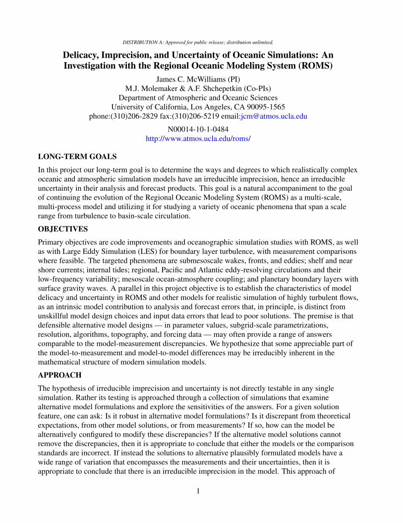
Figure 2 Annual mean sea-surface geostrophic current speed [m sminus1] near the Luzon strait in the Western North Pacific Ocean Indicated with a red solid line is the 03 ms contour level from the AVISO altimetry data set Left and right panels differ only in the land mask for islands at four grid points inside the Luzon strait Local changes in the solution are extremely large In one case the correspondence with AVISO is rather good and in the other it is very poor Similar topographic sensitivity in this region is reported in Hurlburt amp Metzger (GRL 2001) for a different model
11
SRTM30 2011 SRTM30 Jan 2013 GEBCO 08 Sept 2010 GEBCO 1min 2008
ETOPO5 ETOPO2 v1 2001 ETOPO2v2c f4 2006 ETOPO1 Jan 2013
Figure 3 Comparison of bottom topography data from eight datasets used in ocean modeling for the area of Taiwan andthe Luzon Strait
12
Δh = 386m slope=048
Δh = 361m slope=0450
Δh = 335m slope=0416
Δh = 305m slope=0380
Δh = 275m slope=0341
Δh = 240m slope=0293
Figure 4 An example of topographic sensitivity of flow regime in an idealized barotropic island wake f + times u
over sloping bottom Field shown is barotropic potential vorticity BP V = The domain h + ζ
is 320 km long and 80 km wide with a circular island of 20 km in diameter channel configuration The inflow velocity is 015 m sminus1 uniform in horizontal and vertical directions and the Coriolis parameter is f = 10minus4 sminus1 In all the cases the depth is h=500m at the southern side of the domain and it reduces toward the north reaching h minus Δh at the northern side with Δh specified on the left in each panel Also specified is the absolute slope part hpart y expressed in
13
Δt = 60sec M = 17
Δt = 120sec M = 33
Δt = 180sec M = 50
Δt = 200sec M = 55
Figure 5 An example of weak numerical instability caused by inaccurate mode splitting All the conditions are the same as in Fig 4 the second panel from the bottom Δh = 275m except that in this simulation vertically averaged velocity components participating in computation of rhs terms for 3D momentum equations are time centered at nth step (not extrapolated to n + 12) and there is also no recomputing of advective terms at at every time step within the barotropic mode Δt indicated on the left of each panel is the time step for 3D mode and M is the mode splitting ratio (the barotropic time step ΔtM is approximately the same for each panel) Notice a non-physical instability of the wake which is strongly dependent on the size of the time step Consistent mode splitting (either extrapolated vertical averages or recomputed barotropic advective terms) do not exhibit such sensitivity
14

exploring all reasonable formulation alternatives with respect to all relevant solution features is essentially one of exhaustion In practice progress is made by the dual paths of trying to reduce the model discrepancies and educing examples of disconcertingly persistent delicacies in their answers From this experience comes at least provisional assessments of the irreducible uncertainty To address these problems we are making ROMS more of a multi-process multi-purpose multi-scale model by including the coupling of the core circulation dynamics to surface gravity waves sediment resuspension and transport biogeochemistry and ecosystems non-hydrostatic large-eddy simulation and mesoscale atmospheric circulation and by providing a framework for data-assimilation analyses (led by others) In addition we continue to refine the core algorithms for which evidence of solution delicacy is an excellent guide for where improvements may be helpful Furthermore to expand the range of model solutions used to test model sensitivities through collaborations we also use Large Eddy Simulation for the atmospheric and oceanic surface boundary layers (with Peter Sullivan NCAR) the ITCP atmospheric general circulation model (with Annalisa Bracco Georgia Tech) and an intermediate-complexity model of El Ni no ndash Southern Oscillation ENSO (with Mickael Chekroun and David Neelin UCLA)
WORK COMPLETED
In the past year we have worked on the following circulation regimes and phenomena decadal Pacific and Atlantic circulations equilibrium regional circulations in the US West Coast central Alaska Central and South America Solomon Sea the Kuroshio and the Gulf Stream mesoscale eddy buoyancy fluxes submesoscale surface fronts filaments and eddies topographic current separation form stress and submesoscale vortex generation surface waves and nearshore currents and internal tides in Southern California surface wave influences on the turbulent boundary layer and littoral currents bubbles generated by wave breaking mesoscale air-sea coupling using ROMS and WRF the atmospheric general circulation using the ITCP AGCM and the intermediate ENSO model The ROMS algorithmic work has been on adapting the oceanic equation of state for split-explicit time stepping of barotropic and baroclinic modes accurate time-stepping for the bottom boundary layer in shallow water (sim meters) and wake flows past topography open boundary conditions for highly turbulent flows incorporating surface wave effects in ROMS diagnosing spurious diapycnal mixing due to advection errors and designing remedies a new model of a size-distributed bubble population and the exploration of several test-bed configurations for the simulation delicacy investigation
RESULTS
We present a few highlights for this project The publications list (papers from 2012 up to ones likely to be submitted in 2013) provides a view of the finalized results across all our ONR projects
Decision Dilemmas in Parameter Choices An important source of uncertainty in ocean and climate models is linked to the calibration of model parameters Interest in systematic and automated parameter optimization procedures stems from the desire to improve the model climatology and to quantify the average sensitivity associated with potential changes in the climate system Building upon the smoothness of the response of low-order statistical measures of the discrepancy from observations in an atmospheric circulation model (AGCM) to changes of four adjustable parameters Neelin et al (PNAS 2010) used a quadratic metamodel to objectively calibrate the International Centre for Theoretical Physics (ICTP) AGCM The metamodel accurately estimates global spatial averages of common fields of climatic interest from precipitation to low and high level winds from temperature at various levels to sea level pressure and geopotential height while providing a computationally cheap strategy to explore the influence of parameter settings Here guided by the metamodel the ambiguities or dilemmas related to the decision making process in relation to model
2
sensitivity and optimization are examined Global simulations of current climate are subject to considerable regional-scale biases Those biases may vary substantially depending on the climate variable considered andor on the performance metric adopted Common dilemmas are associated with model revisions yielding improvement in one field or regional pattern or season but degradation in another or improvement in the model climatology but degradation in the interannual variability representation Challenges are posed to the modeler by the high dimensionality of the model output fields and by the large number of adjustable parameters The use of the metamodel in the optimization strategy helps visualize trade-offs at a regional level eg how mismatches between sensitivity and error spatial fields yield regional errors under minimization of global objective functions The implication of this analysis is that at least with a modern AGCM the attempt to optimally choose model parameters to reduce its errors with observations encounters severe regional conflicts between improvements for some places and quantities at the cost of degradation in others Pending the creation of a more accurate model the modeler is left with unresolvable dilemmas in the best choice of model parameters which is a type of irreducible uncertainty (Bracco et al 2013)
Rough Parameter Dependences Despite the importance of uncertainties encountered in ocean and climate model simulations the fundamental mechanisms at the origin of sensitive behavior of long-term model statistics remain unclear Variability of turbulent flows in the atmosphere and ocean exhibits recurrent large-scale patterns These patterns while evolving irregularly in time manifest characteristic frequencies across a large range of time scales from intraseasonal through interdecadal Based on modern spectral theory of chaotic and dissipative dynamical systems the associated low-frequency variability (LFV) may be formulated in terms of Ruelle-Pollicott (RP) resonances RP resonances encode information on the nonlinear dynamics of the system and a natural approach for estimating them mdash as filtered through an ldquoobservablerdquo (output variable) of the system mdash is proposed This approach relies on an appropriate Markov representation of the dynamics associated with a given observable It is shown that within this representation the spectral gap mdash defined as the distance between the subdominant RP resonance and the unit circle mdash plays a major role in the roughness of the parameter dependence The model statistics are the most sensitive for the smallest spectral gaps such small gaps turn out to correspond to regimes where the LFV is more pronounced while autocorrelations decay more slowly This approach is applied to analyze the rough parameter dependence encountered in key statistics of an El Ni no - Southern Oscillation model of intermediate complexity (originally due to Jin amp Neelin JAS 1993) It shows that in parameter regimes with greater amplitude for the spontaneous LFV model statistics for some output variables are more sensitive to small changes in the model parameters than they are in regimes with lesser LFV (Fig 1 Chekroun et al 2013) Because the values for model parameters will never be known with high precision a highly rough parameter dependency of model solutions represents an irreducible uncertainty Theoretical arguments strongly suggest that such links between model parameter sensitivity and the decay of correlation properties are not limited to this particular model and could hold much more generally However it may be much more subtle to identify the appropriate observables that display this behavior in a fully realistic general circulation model
Circulation Delicacy due to Wind and Topography Widespread experience in basin-scale oceanic modeling indicates a high degree of sensitivity of strong currents to many aspects of the simulation configuration especially for western boundary currents and their pathway following boundary separation We are exploring the influences of the wind forcing and domain configuration Following the approach described in Lemarie et al (2012a) we have decadal basin-scale ROMS solutions for the Pacific Ocean at a horizontal grid resolution of dx = 125 km and other solutions for the Atlantic Ocean with dx = 7 km For each of these a number of sensitivity experiments have been performed
3
with variations in the wind forcing and the domain shape and topography we restrict ourselves to only plausibly realistic variations ie ones justified by different data sets with alternative interpolation and smoothing procedures to adapt to the model grid In previous annual reports we described remote sensitivities to changes in the wind and topography far away from the separating boundary current Another example is a local topographic sensitivity for the Kuroshio Current as it flows north past Luzon Strait between Taiwan and the Philippines While observations show that there are occasional westward loop intrusions of the Kuroshio into the Strait the pair of solutions in Fig 2 show a much more extreme sensitivity than is observed Motivated by results in Metzger amp Hurlbert (GRL 2001) several islands that were not automatically resolved by the model grid were manually added to the land mask By this alteration in the representation of small islands in the Strait the modeled time-averaged Kuroshio can either cross the Strait or penetrate deeply westward into the South China Sea The latter configuration would be rejected by a modeler on the basis of its embarrassing solution Nevertheless the topographic representation involves somewhat arbitrary and ad hoc decisions about whether to include particular small islands and how to smooth the bathymetric data at a given model resolution Within a less extreme range of model results there may be no physically principled way of eliminating this type of sensitivity apart from further increasing the grid resolution (which may just move the sensitivity to currents on smaller scales) Post hoc selection of the topographic representation based on a particular solution feature here the Kuroshio path would be an unprincipled choice that is likely to increase errors in other features (cf the ldquodecision dilemmardquo above) We are currently working on manuscripts that report the experiences with wind and topographic sensitivities for western boundary currents as well as describe good algorithmic practices for the data handling for the model grid
Treatment of oceanic topography While it is universally accepted that bottom topography plays a major controlling role over oceanic flows the practices associated with handling topography in oceanic models are far from settled at the present time The issues are three-fold (i) uncertainties (and in some cases contradictions) associated with available data sets (ii) procedures associated with preparation of topography for numerical oceanic modeling (iii) topographic sensitivity of numerical algorithms within the oceanic modeling codes The first one (i) is illustrated by Fig 3 We plotted topography from eight different datasets in an identical format using logarithmic scaling to highlight contours in shallow areas At first it is quite striking that consecutive versions of datasets coming from the same source may be radically different without an obvious tendency to converge There is also unexpected historical commonality between some versions taken from the different sources Superficially paying attention to the features between Taiwan and Mainland China the datasets can be categorized into three groups SRTM30 (Jan 2013) GEBCO 08 (Sept 2010) and ETOPO1 (Jan 2013) show a channel-like deeper passage winding toward Mainland and then going along the coast ETOPO2v2c f42006 and GEBCO 1min 2008 show shallow bank protruding from Taiwan toward China (it is somewhat present in ETOPO1 Jan 2013 as well) In our practical experience we found that topography from this group tends to generate ldquohot spotsrdquo (specific places that impose a numerical restriction to maintain stability) between China and Taiwan ETOPO2v1 2001 and SRTM30 2011 just show a rough irregular pattern in the same area Finally we note that even the most modern datasets [GEBCO 08 Sept 2010 SRTM30 Jan 2013 and ETOPO1 Jan 2013] still contain significant differences (up to 500m in depth values of depth) and in features which cannot be explained by differences in interpolation and data quality control The second one (ii) is associated with the fact that in todayrsquos ocean modeling practice topographic datasets are available at resolutions which are typically higher than model grids This means that the data must be essentially coarsened which unavoidably leads to suppression of some topographic
4
features The mathematical optimization dilemma of how to keep model topography representative of the realistic one but at the same time numerically acceptable by the modeling code is not uniquely solvable For example smoothing of a ridge while conserving its volume unavoidably leads to the reduction of its height which changes the regime by opening a path which should not be open On the other hand maintaining the height while reducing the steepness of the slopes leads to an increase of volume which still may be preferred It is not surprising that historical publications related to this subject (eg Mellor et al JAOT 1994 Martinho amp Batteen OM 2006 Sikiric et al OM 2009) advocate very different criteria We have developed robust techniques for transferring data topography into model grid (including both averagingdealiasing and enforcing numerical slope constraints) however the main criterion of success remains the behavior of modeled flow as the result of simulation rater than satisfying an a priori selected constraint This leaves a degree of empiricism and an unavoidable imprecision Figure 4 illustrates sensitivity of the flow regime to topographic slope in a superficially simple case of barotropic flow past and obstacle ndash a cylindrical island The slope is rather gentle and there are no numerical concerns about the accuracy of this simulation Yet the flow regime changes in an unintuitive way with a smoothly changing controlling parameter When the slope is weak (bottom panel) the pattern is similar to a vortex street with cyclonic and anticyclonic eddies alternately shed from the left and right side of the island Once the slope reaches a certain value (034 to 038) no eddies are shed and the wake only oscillates slightly around the midline Further increase of the slope leads to a highly non-stationary regime again While the mechanism of such change cannot be fully explained we note that increase of the slope results in proportional increase of the speed of topographic Rossby waves which at some point match the inflow velocity (in this configuration Rossby waves propagate upstream) resulting in qualitatively distinct below match and above regimes while no further qualitative changes are expected outside this range of parameters (experiments with opposite-sign slope reveal no special behavior) Code algorithmic sensitivity to topography item (iii) is a widely known topic (eg sigma-coordinate pressure-gradient errors spurious mixing) yet some of its aspects are much less noted Theoretical studies of the stability of barotropic-baroclinic mode splitting stay entirely within the consideration of linear internal and external waves in layered systems over a flat bottom (Higdon amp Bennett JCP 1996 et seq) Practical oceanic modeling requires nonlinear advection topography and mode splitting Figure 5 shows a numerical instability associated with improper computation of advection terms due to splitting In principle this type of instability occurs even without topography but with topography it was first pointed out by Morel et al (OM 2008) in the context of HYCOM (they propose a remedy) but in fact this would occur in every existing modeling code that does not recompute advection terms within the barotropic mode (eg MOM POP etc ) Originally ROMS and POM do so (hence are not subject to such instability) however this clearly comes with extra computational cost so we have redesigned the code for efficiency while having an approach different from that of Morel et al (2008)
IMPACTAPPLICATIONS
Geochemistry and Ecosystems An important community use for ROMS is biogeochemisty chemical cycles water quality blooms micro-nutrients larval dispersal biome transitions and coupling to higher tropic levels We collaborate with Profs Keith Stolzenbach (UCLA) Curtis Deutsch (UCLA) David Siegel (UCSB) and Yusuke Uchiyama (Kobe) Data Assimilation We collaborate with Drs Zhinjin Li (JPL) Yi Chao (Remote Sensing Solutions) and Kayo Ide (U Maryland) by developing model configurations for targeted regions and by consulting on the data-assimilation system design and performance Current quasi-operational 3DVar applications are in California (SCCOOS and CenCOOS) and in Alaska (Prince William Sound)
5
TRANSITIONS
ROMS is a community code with widespread applications (httpwwwmyromsorg)
RELATED PROJECTS
Three Integrated Ocean Observing System (IOOS) regional projects for California and Alaska (SCCOOS CenCOOS and AOOS) utilize ROMS for data assimilation analyses and forecasts
6
PUBLICATIONS
Bracco A J D Neelin H Luo J C McWilliams and J E Meyerson 2013 High dimensional decision dilemmas in climate models Geosci Model Dev 6 2731-2767 doi105194gmdd-6-2731-2013
Buijsman MC Y Uchiyama J C McWilliams and C R Hill-Lindsay 2012 Modeling semidiurnal internal tide variability in the Southern California Bight J Phys Oceanogr 42 62-77 doi1011752011JPO45971
Chekroun M D J D Neelin D Kondrashov J C McWilliams and M Ghil 2013 Rough parameter dependence in climate models The role of Ruelle-Pollicott resonances Proc Nat Acad Sci submitted
Colas F JC McWilliams X Capet and J Kurian 2012 Heat balance and eddies in the Peru-Chile Current System Climate Dynamics 39 509-529 doi101007s00382-011-1170-6
Colas F X Capet JC McWilliams and Z Li 2013a Mesoscale eddy buoyancy flux and eddy-induced circulation in eastern boundary currents J Phys Oceanogr 43 1073-1095 doi101175JPO-D-11-02411
Colas F X Wang X Capet Y Chao and JC McWilliams 2013b Untangling the roles of wind run-off and tides in Prince William Sound Continen Shelf Res 63 S79-S89 doi101016jcsr201205002
Dong C X Lin Y Liu F Nencioli Y Chao Y Guan T Dickey and J C McWilliams 2012 Three-dimensional oceanic eddy analysis in the Southern California Bight from a numerical product J Geophys Res 117 C00H14 doi1010292011JC007354
Farrara J Y Chao Z Li X Wang X Jin H Zhang P Li Q Vu P Olsson C Schoch M Halverson M Moline C Ohlmann M Johnson J C McWilliams and F Colas 2013 A data-assimilative ocean forecasting system for the Prince William Sound and an evaluation of its performance during Sound Predictions 2009 Continental Shelf Research 63 S193-S208 doi101016jcsr201211008
Gula J M J Molemaker and J C McWilliams 2013a Mean dynamic balances in the Gulf Stream in high-resolution numerical simulations in preparation
Gula J M J Molemaker and J C McWilliams 2013b Gulf Stream dynamics and frontal eddies along the Southeast US continental shelf in preparation
Gula J M J Molemaker and J C McWilliams 2013c Submesoscale cold filaments in the Gulf Stream in preparation
Gula J M J Molemaker and J C McWilliams 2013d Submesoscale instabilities on the Gulf Stream north wall in preparation
Lemarie F J Kurian AF Shchepetkin MJ Molemaker F Colas and J C McWilliams 2012a Are there inescapable issues prohibiting the use of terrain-following coordinates in climate models Ocean Modelling 42 57-79 doi101016jocemod201111007
Lemarie F L Debreu L AF Shchepetkin and JC McWilliams 2012b On the stability and accuracy of the harmonic and biharmonic adiabatic mixing operators in ocean models Ocean Modelling 52-53 9-35 doi101016jocemod201204007
Li Z Y Chao J Farrara and J C McWilliams 2013 Impacts of distinct observations during the 2009 Prince William Sound field experiment A data assimilation study Continental Shelf Research 63 S209-S222 doi101016jcsr201206018
7
Li Z Y Chao J McWilliams K Ide and J D Farrara 2012 A multi-scale three-dimensional variational data assimilation and its application to coastal oceans Q J Roy Met Soc submitted
Li Z Y Chao JC McWilliams K Ide and J Farrara 2012 Experiments with a multi-scale data assimilation scheme Tellus Series A Dynamic Meteorology and Oceanography submitted
Liang J-H J C McWilliams P P Sullivan and B Baschek 2012 Large Eddy Simulation of the bubbly ocean Impacts of wave forcing and bubble buoyancy J Geophys Res 117 C04002 doi1010292011JC007766
Liang J-H J C McWilliams J Kurian P Wang and F Colas 2012 Mesoscale variability in the Northeastern Tropical Pacific Forcing mechanisms and eddy properties J Geophys Res 117 C07003 doi1010292012JC008008
Liang J-H C Deutsch J C McWilliams B Baschek P P Sullivan and D Chiba 2013 Parameterizing bubble-mediated air-sea gas exchange and its effect on ocean ventilation Glob Biogeo Cycles 27 doi101002gbc20080
McWilliams J C E Huckle J Liang and P P Sullivan 2012 The wavy Ekman layer Langmuir circulations breakers and Reynolds stress J Phys Oceanogr 42 1793-1816 doi101175JPO-D-12-071
McWilliams J C and B Fox-Kemper 2013 Oceanic Wave-balanced surface fronts and filaments J Fluid Mech 730 464-490 doi101017jfm2013348
McWilliams J C E Huckle J Liang and P P Sullivan 2013 Langmuir Turbulence in swell J Phys Oceanogr submitted
Mechoso C R R Wood R Weller C S Bretherton A D Clarke H Coe C Fairall J T Farrar G Feingold R Garreaud C Grados J McWilliams S P de Szoeke S E Yuter and P Zuidema 2013 Ocean-Cloud-Atmosphere-Land Interactions in the Southeastern Pacific The VOCALS Program Bull Amer Met Soc doi101175BAMS-D-11-002461
Menesguen C J C McWilliams and M J Molemaker 2012 An example of ageostrophic instability in a rotating stratified flow J Fluid Mech 711 599-619 doi101017jfm2012412
Molemaker M J J C McWilliams and W K Dewar 2013 Submesoscale instability and generation of mesoscale anticyclones near a separation of the California Undercurrent J Phys Oceanogr submitted
Molemaker M J J C McWilliams and W K Dewar 2013 Centrifugal instability and mixing in the California Undercurrent J Phys Oceanogr submitted
Romero L Y Uchiyama J C Ohlmann J C McWilliams and D A Siegel 2013 Simulations of nearshore particle-pair dispersion in Southern California J Phys Oceanogr 43 1862-1879 doi101175JPO-D-13-0111
Roullet G J C McWilliams X Capet and M J Molemaker 2012 Properties of equilibrium geostrophic turbulence with isopycnal outcropping J Phys Oceanogr 42 18-38 doi101175JPO-D-11-091
Shcherbina A Y E A DrsquoAsaro C M Lee J M Klymak M J Molemaker and J C McWilliams 2013 Statistics of vertical vorticity divergence and strain in a developed submesoscale turbulence field Geophys Res Lett 40 doi101002grl50919
Sullivan P P L Romero J C McWilliams and W K Melville 2012 Transient evolution of Langmuir Turbulence in ocean boundary layers driven by hurricane winds and waves J Phys
8
Oceanogr 42 1959-1980 doi101175JPO-D-12-0251 Sullivan P P J C McWilliams and E G Patton 2013 A high-Reynolds number Large Eddy
Simulation model of the marine atmospheric boundary layer above a spectrum of moving waves in preparation
Uchiyama Y E Idica J C McWilliams and K Stolzenbach 2013 Wastewater effluent dispersal in two Southern California Bays Cont Shelf Res submitted
Wang P J C McWilliams and Z Kizner 2012 Ageostrophic instability in rotating shallow water J Fluid Mech 712 327-353 doi101017jfm2012422
Wang P J C McWilliams and C M enesguen 2013 Ageostrophic instability in rotating stratified interior vertical shear flows J Fluid Mech submitted
Wang X Y Chao H Zhang J Farrara Z Li X Jin K Park F Colas J C McWilliams C Paternostro CK Shum Y Yi C Schoch and P Olsson 2013 Modeling tides and their influence on the circulation in Prince William Sound Alaska Continental Shelf Research 63 S126-S137 doi101016jcsr201208016
9
FIGURES
Figure 1 Statistical sensitivity of the Ni no-3 SST ldquoobservablerdquo in an intermediate complexity model of El Ni no - Southern Oscillation Plotted are relative changes in percentage for the standard deviation (STD) and skewness with respect to variations in δ a parameter affecting the trans-Pacific travel time of equatorial ocean waves Panels (a) and (c) correspond to a model parameter-set that yields a ldquorapidly mixingrdquo regime with little low-frequency variability (LFV) and they show relatively smooth variations with δ except for a few bifurcation points Panels (b) and (d) correspond to a ldquoslowly mixingrdquo regime with more LFV In each of these panels the chaotic (resp periodic or quasi-periodic) behavior is represented by red (resp black) dots In panel (d) two consecutive cyan dots represent local changes in the skewness from about 95 to 135 for corresponding variations in δ of less than 006 (Chekroun et al 2013)
10
Figure 2 Annual mean sea-surface geostrophic current speed [m sminus1] near the Luzon strait in the Western North Pacific Ocean Indicated with a red solid line is the 03 ms contour level from the AVISO altimetry data set Left and right panels differ only in the land mask for islands at four grid points inside the Luzon strait Local changes in the solution are extremely large In one case the correspondence with AVISO is rather good and in the other it is very poor Similar topographic sensitivity in this region is reported in Hurlburt amp Metzger (GRL 2001) for a different model
11
SRTM30 2011 SRTM30 Jan 2013 GEBCO 08 Sept 2010 GEBCO 1min 2008
ETOPO5 ETOPO2 v1 2001 ETOPO2v2c f4 2006 ETOPO1 Jan 2013
Figure 3 Comparison of bottom topography data from eight datasets used in ocean modeling for the area of Taiwan andthe Luzon Strait
12
Δh = 386m slope=048
Δh = 361m slope=0450
Δh = 335m slope=0416
Δh = 305m slope=0380
Δh = 275m slope=0341
Δh = 240m slope=0293
Figure 4 An example of topographic sensitivity of flow regime in an idealized barotropic island wake f + times u
over sloping bottom Field shown is barotropic potential vorticity BP V = The domain h + ζ
is 320 km long and 80 km wide with a circular island of 20 km in diameter channel configuration The inflow velocity is 015 m sminus1 uniform in horizontal and vertical directions and the Coriolis parameter is f = 10minus4 sminus1 In all the cases the depth is h=500m at the southern side of the domain and it reduces toward the north reaching h minus Δh at the northern side with Δh specified on the left in each panel Also specified is the absolute slope part hpart y expressed in
13
Δt = 60sec M = 17
Δt = 120sec M = 33
Δt = 180sec M = 50
Δt = 200sec M = 55
Figure 5 An example of weak numerical instability caused by inaccurate mode splitting All the conditions are the same as in Fig 4 the second panel from the bottom Δh = 275m except that in this simulation vertically averaged velocity components participating in computation of rhs terms for 3D momentum equations are time centered at nth step (not extrapolated to n + 12) and there is also no recomputing of advective terms at at every time step within the barotropic mode Δt indicated on the left of each panel is the time step for 3D mode and M is the mode splitting ratio (the barotropic time step ΔtM is approximately the same for each panel) Notice a non-physical instability of the wake which is strongly dependent on the size of the time step Consistent mode splitting (either extrapolated vertical averages or recomputed barotropic advective terms) do not exhibit such sensitivity
14