improved double default modeling for the basel framework ... · improved double default modeling...

Improved Double Default Modeling for the Basel Framework -An Endogenous Asset Drop Model without Additional Correlation

Sebastian EbertBonn Graduate School of Economics, University of Bonn Adenauerallee 24-42 53113 Bonn,

Germany. Tel.: +49 228 739225; Fax: +49 228 735048.Email address: [email protected]

Eva LutkebohmertInstitute for Research in Economic Evolution, University of Freiburg, Platz der Alten Synagoge,

79085 Freiburg, Germany. Tel.: +49 761 2039362.

Email address: [email protected]

Abstract. In 2005 the Internal Ratings Based (IRB) approach of ‘Basel II’

was enhanced by a ‘treatment of double default effects’ to account for credit

risk mitigation techniques such as ordinary guarantees or credit derivatives.

This paper reveals several severe problems of this approach and presents a new

method to account for double default effects. This new asset drop technique

can be applied within any structural model of portfolio credit risk. When

formulated within the Basel framework’s IRB approach, it is very well suited

for practical application as it does not pose extensive data requirements and

economic capital can still be computed analytically.

Key words: Basel capital accord, double default, IRB approach, regulatory capital,structural credit portfolio models

JEL Codes: G31, G28

Acknowledgements. Both authors acknowledge the financial support from the BonnGraduate School of Economics and from the German Research Foundation through theproject “Pricing of Risk in Incomplete Markets” at the University of Freiburg. The authorsvery much appreciate several helpful comments and suggestions from John O’Keefe, whodiscussed the paper at the 2009 Australasian Banking and Finance Conference in Sydney.We also thank conference participants at the Bachelier World Congress 2010 (Toronto) andat the Financial Risks International Forum 2010 (Paris), as well as seminar participants atthe Universities of Bonn and Freiburg. The authors are very grateful to Thomas Gehrigfor several helpful comments.

1

1. Introduction

In 2005 the Basel Committee of Banking Supervision (BCBS) made an amendment

(BCBS, 2005) to the original New Basel Accord of 2003 (BCBS, 2003) that deals with the

treatment of hedged exposures in credit portfolios.1 In the original New Basel Accord of

2003, banks are allowed to adopt a so-called substitution approach to hedged exposures.

Roughly speaking, under this approach a bank can compute the risk-weighted assets for

a hedged position as if the credit exposure was a direct exposure to the obligor’s guar-

antor. Therefore, the bank may have only a small or even no benefit in terms of capital

requirements from obtaining the protection. Since the 2005 amendment, for each hedged

exposure the bank can choose between the substitution approach and the so-called double

default treatment. The latter, inspired by Heitfield and Barger (2003), takes into account

that the default of a hedged exposure only occurs if both the obligor and the guaran-

tor default (“double default”) thus seems to be more sophisticated and realistic than the

substitution approach.

The recent global financial crisis drastically demonstrated the importance of how to

treat hedged exposures in credit portfolios. However, the literature on the treatment of

double default effects within the computation of economic capital is scarce. This is par-

ticularly true for the literature on the computation of regulatory capital under Basel II.

Given that the former model sets a benchmark for the quantification of minimal capital

requirements for hedged exposures of banks in the European Union, this seems to be un-

justified.

There is no doubt that hedging exposures is rather a natural act than a rare exception.

For example, granting loans and transferring the risk afterwards is a typical business for a

bank. This can be done by use of numerous instruments (referred to as credit risk mitiga-

tion (CRM) techniques in Basel II) such as ordinary guarantees, collateral securitization

and credit derivatives (in particular credit default swaps and bundled credit packages such

as credit loan obligations), to name a few.2 This is also why CRM techniques were dis-

cussed extensively in Basel II in the first place and why the Basel Committee chose to

improve on the earlier version by introducing the treatment of double default effects in

1Meanwhile the amendment also has been incorporated in a revised version of the 2003 New BaselAccord, BCBS (2006). If not noted otherwise, this is the version we refer to with “Basel II”.2The market for credit derivatives has grown rapidly in the years preceding the crisis. Accordingto a survey of the International Swaps and Derivatives Association published on April 22, 2009,the notional of outstanding CDSs was US$39 trillion as of December 2008.

IMPROVED DOUBLE DEFAULT MODELING FOR THE BASEL FRAMEWORK 3

2005. After all, through the regulatory treatment of double default effects, the BCBS sets

incentives for banks to obtain credit protection. In the aftermath of the global financial

crisis, the BCBS again is largely concerned with making improvements to the treatment

of counterparty risk in Basel II in general (see BCBS, 2009). However, in that document

and those building up on it, which are sometimes summarized under the term ‘Basel III’,

the BCBS has not addressed the treatment of double default effects. In this paper, we

motivate and propose a new methodology to treat double default effects in any structural

credit risk model. In particular, we are concerned with the computation of regulatory

capital in the IRB approach of Basel II.3

To motivate our new method, we first review the Internal Ratings Based (IRB) treat-

ment of double default effects. While this approach constitutes an important first step

in modeling double default under Basel II, we will show that it also has severe shortcom-

ings. Most importantly, we argue that imposing additional correlation between obligors

and guarantors is unsuitable to capture their essentially asymmetric relationship appro-

priately. We also show that this approach, in general, violates some of the assumptions

of the Asymptotic Single Risk Factor (ASRF) model (see Gordy, 2003) which represents

the mathematical basis of the IRB approach. Furthermore, it is implicitly assumed within

the IRB treatment of double defaults that guarantors are external. That is, it is assumed

that there is no direct exposure to guarantors. It is also assumed that every loan in the

portfolio is hedged by a different guarantor. This leads to an underestimation of the as-

sociated concentration risk.

The major contribution of this paper is a new method to account for double default effects

in the computation of economic capital. It can be used within all structural models of

credit risk and, in particular, in the IRB approach of Basel II. The model does not exhibit

any of the deficiencies we point out for the IRB treatment of double defaults. Instead of

modeling the relationship between an obligor and its guarantor through a dependency on

an additional stochastic risk factor, we adjust the guarantor’s default probability appro-

priately if the hedged obligor defaults. The model is endogenous as it actually quantifies

3As the IRB approach has been part of the Basel II reforms, we speak of our proposed treatment asbeing an improvement to the IRB approach of Basel II. Of course, our treatment likewise applies

to Basel III as the model underlying the IRB approach has not been changed.

4 IMPROVED DOUBLE DEFAULT MODELING FOR THE BASEL FRAMEWORK

the increase of the guarantor’s default probability instead of exogenously imposing a nu-

merical value as it is done in the IRB treatment of double default effects for the additional

correlation parameters. The idea behind the model is to quantify the size of the downward

jump of the guarantor’s firm value process in case of the obligor’s default which triggers

the guarantee payment. We therefore call this approach an asset drop model. Practical

application of the model is straightforward since it does not require extensive data. More-

over, due to its simple analytic representation, economic capital can be computed almost

instantaneously.

Structural models with (downward) jumps have been considered previously in the lit-

erature, e.g. in case of the jump diffusion model of Zhou (2001b). Bivariate versions of

the latter were introduced in Zhou (2001a) and Hull and White (2001). These approaches

have also been used to model default dependencies in the counterparty risk literature,

in particular for evaluating the credit value adjustment (CVA) for credit default swaps

(CDSs). See, for example, Lipton and Sepp (2009) and Brigo and Chourdakis (2009), and

references therein. In these models jumps occur randomly rather than being triggered by

a specific event as in our model. That is, we provide an explanation for the jump time

as well as for the jump size. Moreover, in contrast to our approach the above mentioned

literature models dependencies symmetrically by correlating the asset processes. Most

importantly, none of the papers deals with the computation of regulatory capital.

Parts of the CVA literature (e.g. Pykhtin and Zhu, 2007, Gregory, 2009 and Pykhtin,

2010) explicitly focus on the estimation of exposure at default (EAD), i.e. on estimating

the loss in market value when the contract terminates. Similarly, Taplin et al. (2007) and

Valvonis (2008) investigate the credit conversion factor used to account for possible (re-

tail) overdrafts. This literature can be understood as being complementary to our work,

also in order to consider the price, value and market risk of a guarantee. Similarly, one

could calculate the refinancing costs that occur if a guarantor defaults and the guarantee

should be reestablished. If a collateral serves as a guarantee, the jump size could be taken

as its exposure at default.

Closer to our model is the contagion model of Leung and Kwok (2005). There, upward

jumps in the default intensity of an entity occur whenever another entity defaults. This

allows for an asymmetric dependency structure between obligor and guarantor, which has


to be specified exogenously.

While the mentioned literature focuses on the proper pricing of guarantees like CDSs by

evaluating the CVA, our paper deals with the impact of guarantees on regulatory capital.

That is, once the guarantee has been obtained (no matter what its price, CVA or current

market value is), by how much should credit risk sensitive regulatory capital be reduced?

Although the IRB treatment of double default effects is largely applied in practice, this

question has not been answered so far. To the best of our knowledge the only other paper

that is directly addressing the IRB model of double default is Grundke (2008). The latter,

however, is not concerned with the IRB model itself and its assumptions, but rather with

the appropriate parameter choices within the model of Heitfield and Barger (2003).

The remainder of the paper is structured as follows. In Section 2 we provide a review

of the Internal Ratings Based (IRB) treatment of double default effects and we reveal

several severe shortcomings of the approach. Section 3 contains our new asset drop model

to account for double default effects which can be used in all structural models of credit

risk and, in particular, in the IRB approach of Basel II. We also implement our method

within some examples and compare the results to the current IRB treatment of double

default effects. The discussion and conclusions of the paper are given in Section 4.

2. Review and Discussion of the IRB Treatment of Double Defaults

Within the IRB approach of Pillar 1 in Basel II banks may choose between the simple

substitution approach outlined in the Introduction and a double default approach where

risk-weighted assets for exposures subject to double default are calculated as follows.4

Assume the exposure to obligor n is hedged by guarantor gn. Within the double default

treatment in the IRB approach one first computes the unexpected loss (UL) capital re-

quirement Kn for the hedged obligor n in the same way as the one for an unhedged

exposure5 with LGDn replaced by the loss given default LGDgn of the guarantor. In the

computation of the maturity adjustment the default probability is chosen as the min-

imum of the obligor’s default probability PDn and the guarantor’s default probability

PDgn . Then the UL capital requirement KDDn for the hedged exposure is calculated by

4Compare BCBS (2006), paragraph 284.5The latter is defined in paragraphs 272 and 273 of BCBS (2006).


multiplying Kn by an adjustment factor depending on the PD of the guarantor, namely

(1) KDDn = Kn · (0.15 + 160 · PDgn).

Finally, the risk-weighted asset amount for the hedged exposure is computed in the same

way as for unhedged exposures. Note that the multiplier (0.15 + 160 · PDgn) is derived

as a linear approximation to the UL capital requirement for hedged exposures. For the

computation of the latter, i.e. to derive the exact conditional expected loss function for a

hedged exposure, the ASRF framework, which also presents the basis for the computation

of the risk weighted assets in the IRB approach, is used in an extended version. Specifically,

it is assumed that the asset returns rn (resp. rgn) of an obligor and its guarantor are no

longer conditionally independent given the systematic risk factor X but also depend on

an additional risk factor Zn,gn which only affects the obligor and its guarantor. More

precisely,

(2) rn =√ρnX +

√1− ρn

(√ψn,gnZn,gn +

√1− ψn,gnεn

),

where ρn is the asset correlation of obligor n, ψn,gn is a factor specifying the sensitivity

of obligor n to the factor Zn,gn and εn is the idiosyncratic risk factor of obligor n. By

implicitly assuming that all hedges are perfect full hedges, guarantors are themselves not

obligors in the portfolio and different obligors are hedged by different guarantors, the joint

default probability of the obligor and its guarantor can be computed explicitly as6

(3)P ({default of obligor n} ∩ {default of guarantor gn})

= Φ2

(Φ−1(PDn),Φ−1(PDgn); ρn,gn

),

where ρn,gn is the correlation between obligor n and its guarantor gn and Φ2(·, ·; ρ) denotes

the cumulative distribution function of the bivariate standard normal distribution with

correlation ρ. Therefore, the conditional expected loss function for a hedged exposure is

given by

(4)

E[1l{rn≤cn}1l{rgn≤cgn} LGDn LGDgn |X

]= LGDn LGDgn ·

·Φ2

(Φ−1(PDn)−√ρnX√

1− ρn,

Φ−1(PDgn)−√ρgnX√1− ρgn

;ρn,gn −

√ρnρgn√

(1− ρn)(1− ρgn)

)for default thresholds cn and cgn for obligor n and its guarantor gn, respectively. One

obtains the IRB risk weight function for a hedged exposure with effective maturity of one

year by inserting Φ−1(0.001) for X, subtracting the expected loss

(5) Φ2(Φ−1(PDn),Φ−1(PDgn); ρn,gn) · LGDn LGDgn

6For more details on the derivation see for example Grundke (2008), pp. 40-41.


and multiplying with 12.5 and 1.06. Since the expected loss should in general be rather

small, in BCBS (2005) this term is set equal to zero. Moreover, it is assumed that there

are no double recovery effects and thus LGDn = 1. Within the IRB treatment of double

default effects, however, the linear approximation (1) of the exact conditional expected

loss function (4) is used which holds for the parameter values specified before.7

Let us now discuss the assumptions underlying this approach in more detail. First

let us investigate how well correlation in general suits to model the dependency between

a guarantor and an obligor. Positive correlation implies that the default of the obligor

makes the default of the guarantor more likely. This seems very reasonable as the guar-

antor suffers from the guarantee payment, and if it is large it might even drag him into

default. Vice versa, however, it seems neither theoretically nor empirically justified that

the default of the guarantor implies a similar pain to the hedged obligor.8 Note that the

obligor in general will not even know whether the bank that granted the loan obtained

credit protection at all. And if so, the obligor will not know the name of the guarantor.

Essentially, for the hedged obligor the pain from the default of the guarantor should be not

larger than the pain from the default of any other firm in the economy. It will influence

the default probability of the obligor only through shifts in the state of the systematic

risk factor. As correlation necessarily introduces a symmetric dependency between two

random variables, it can never capture appropriately the asymmetric relationship that

holds between a guarantor and an obligor.

Before we continue, let us first consider a case where modeling the dependency between

a guarantor and an obligor symmetrically could be justified. Suppose, first, there is no

direct exposure to guarantors and, second, every guarantor hedges exactly one position in

the portfolio. In this case one is interested in the double default but otherwise not in the

default of the guarantor. The unconditional dependence of the guarantor with the rest of

the portfolio is ignored, but this can be compensated perfectly by choosing the additional

correlation sufficiently high. Essentially, in this case the obligor and its guarantor (that

7Grundke (2008) explains this approximation in more detail and illustrates its accuracy. For acomprehensive and more detailed overview of the double default treatment we refer to his paper

and the original paper by Heitfield and Barger (2003).8For a discussion of wrong-way risk and the market risk of guarantees see Remark 2 at the end ofthis section.


interacts with the obligor and nobody else) constitute a conditionally independent unit in

the portfolio. Then correlation can be used reasonably to model the default dependency

between the obligor and its guarantor and the default event of obligor 1 can be simply

replaced with the less likely double default event.

The IRB treatment of double default effects simply makes no distinction, whether or not

a guarantor is itself an obligor in the portfolio or if it guarantees for several obligors. The

implicit approach undertaken in the IRB model for any hedging constellation is the one

just explained.

If one of the two assumptions above is violated, an application of the IRB treatment of

double default effects is no more rigorous. When applying the IRB treatment of double

defaults, the interactions of each guarantor with the rest of the portfolio are ignored. To

be more precise, if the guarantor itself is in the portfolio, it would be treated as any

other obligor in the portfolio, in particular conditionally independent from the obligor it

guarantees for. Its expected loss is computed as if it was not involved in a hedging rela-

tionship, i.e. with an unchanged default probability and a correlation parameter as used

for obligors rather than guarantors. If a guarantor hedges several positions this problem

becomes even more severe. Moreover, this implies that overly excessive contracting of the

same guarantor is not reflected in the computation of economic capital.

Further note that the IRB treatment of double default effects is generally unsuited to deal

with the above situations because of the additional correlation assumption. If the guar-

antor is itself in the portfolio, its default will significantly increase the default probability

of the obligor, what, as mentioned before, is an unappreciated consequence. If on the

other hand the guarantor hedges more than one obligor, say 3 hedges 1 and 2, then the

default of 1 increases the guarantor’s default probability which itself increases the default

probability of 2. That is, 1 and 2 are no more conditionally independent because they

share the same ‘contagious’ guarantor. In general, this seems to be very unreasonable as

there need not be any business relationship between 1 and 2 or there even might be a

negative relationship between them such that the default of 1 should actually decrease

the default probability of obligor 2.9 Thus we conclude that the IRB treatment of double

default effects can only be used reasonably if every obligor in the portfolio has a different

guarantor and if there is no direct exposure to any of those guarantors.

9Similarly to the argument before, also note that 1 and 2 will not know wether there is a guarantor.And if so, they will not know who it is.


Remark 1. (Consistency with the ASRF model.) From a theoretical or mathematical

point of view introducing additional correlation within the IRB approach leads to some

problems as a main assumption underlying this framework is violated. Suppose that a

guarantor hedges several obligors or that a guarantor is internal in the sense that there is

also direct exposure to the guarantor. In this case the additional correlation violates the

conditional independence assumption, on which the ASRF model is based. Conditional

independence between the obligor loss variables, however, is required as the ASRF model

relies on a law of large numbers. Let us mention here, however, that the violation of the

conditional independence assumption underlying the ASRF model will essentially occur

in any approach that correctly accounts for the interactions resulting from double default

effects. The asymptotic result used in the approximation of the value-at-risk αq(L) of the

portfolio loss by the expected portfolio loss E[L|αq(X)] conditional on the quantile αq(X)

of the systematic risk factor in this situation only holds when the hedged exposure shares

and the direct exposure shares to guarantors are sufficiently small.

Finally, let us also mention another deficiency of the IRB treatment of double default

effects which is highly relevant for practical applications. It concerns the parameter choice

of the conditional correlation parameters. While not questioning the assumption of im-

posing additional correlation between an obligor and its guarantor in general, in a recent

and long overdue empirical study, Grundke (2008) investigates the numerical values of the

correlation parameters ρgn = 0.7 and ρn,gn = 0.5 set by the BCBS. To this purpose, he re-

views empirical studies on default correlation and further initiates new simulation studies,

which yield rather different results. While the empirical studies he considers imply that

the parameters are chosen overly conservative, the simulation experiments “show that the

assumed values are not unrealistic for capturing the intended effects”.10 He also notes

that the appropriateness of the parameter choice actually depends, for example, on the

size of the guarantor and the amount guaranteed. Within the IRB treatment of double

default effects the correlation parameters are independent of these quantities. Implicitly

this means, for instance, that a small bank and a large insurance company would suffer

equally from any guarantee payment.

10See p. 58 of Grundke (2008).


Remark 2. (Wrong-way risk.) It might be argued that not the obligor, but the bank

whose regulatory capital we aim to compute will be affected by the guarantor’s default.

This phenomenon, sometimes referred to as ‘wrong-way risk’, might be due to a loss

in market value of the defaulted hedging product. For example, if the bank decides

to obtain a new guarantee, this loss in market value had to be realized immediately as

replacement costs. It should be clear, however, that this effect will not justify a symmetric

dependency structure.11 Moreover, we propose not to dilute this effect with the Pillar 1

capital requirements. Also in the current treatment of double default effects within the

IRB approach the price or market value of guarantees is not reflected, and this seems

well justified. Given the existence of the guarantee, the bank should benefit from smaller

capital requirements (depending on the quality of the guarantee). If there is no guarantee

(or of it has defaulted), it should not. Price, market value or possible replacement costs of

the guarantee should be reflected on the market risk side. The CVA literature mentioned

in the introduction offers appropriate tools for its risk assessment.

3. The Asset Drop Technique as an Alternative Approach

In this section we will present an alternative method to account for double default

effects in credit portfolios that does not rely on additional correlation between obligor and

guarantor. It does capture their asymmetric relationship, i.e. that the guarantor should

suffer much more from the obligor’s default (triggering the guarantee payment) than vice

versa. Further, our method distinguishes the case where there is direct exposure to the

guarantor from the case where it is external to the portfolio. Furthermore, we properly

treat the situation where a guarantor hedges several obligors.

Instead of modeling the relationship between guarantor and obligor through a dependency

on an additional stochastic risk factor, we adjust the guarantor’s default probability ap-

propriately if the obligor defaults. Our model is endogenous as it actually quantifies the

increase of the guarantor’s default probability instead of exogenously imposing numeri-

cal values as it is done in case of the additional correlation parameters ρn,gn in the IRB

treatment of double default effects. The increase in the guarantor’s default probability in

our new approach depends on the size of the guarantee payment as well as on the size of

the guarantor measured in terms of its asset value. The method is very well suited for

11Within the model we will propose it is straightforward to incorporate such a reverse feedbackeffect while still having some asymmetry. This can be achieved e.g. by introducing an additionaldrop in the asset value of the obligor by the market value of the hedging product.


practical applications as it does not pose any extensive data requirements. Moreover, due

to its simple analytic representation of economic capital when incorporated in the IRB

model, it can be computed almost instantaneously.

3.1. Methodology. Within a structural model of default, the guarantee payment that

occurs to the guarantor corresponds to a downward jump in its firm value process or,

equivalently, in the firm’s asset return. This causes the unconditional default probability

to increase by a growth factor (1 + λn,gn). This qualitative observation can be found in

Grundke (2008), p. 53.12 To illustrate the idea of the approach, let us first consider the

simple case where obligor 1 is hedged by a guarantor, g1, which is external to the portfolio.

That is, the guarantor is itself not an obligor in the portfolio. We want to quantify the

impact of obligor 1’s default on the guarantor’s unconditional default probability. In the

current situation the default of the guarantor is only of interest if obligor 1 defaults as

well. If solely the guarantor defaults there is no loss as there is no direct exposure to the

guarantor. Thus, our objective is to compute the guarantor’s (increased) default proba-

bility when the hedged obligor already has defaulted such that the guarantee payment has

been triggered. The loss due to the guarantee payment may cause the guarantor’s default

or may make it more likely. For simplicity and for consistency with the IRB approach

we illustrate the method within an extension of the model of Merton (1974). However,

in principle our new approach can also be applied in more sophisticated structural credit

risk models which are e.g. driven by Levy processes.

In the IRB approach we consider a two-period model with a 1-year horizon where time

t is today and T refers to one year in the future. Our input parameters are the initial

firm value Vg1(t) of the guarantor g1, i.e. the firm’s value at time t taken e.g. from the

balance sheet or inferred from the current stock price, as well as an estimate of its volatility

σg1 . We further need the (non-portfolio specific) default probability PDg1 , that could be

obtained from a rating agency, and the risk-free interest rate r. In Merton’s model it is

assumed that the asset value process of guarantor g1 follows a geometric Brownian motion

12In order to assess the conservativeness of the parameter choices for the additional correlation

in the treatment of double default effects in the IRB approach, Grundke (2008) shows that the

additional correlation approximately translates into an increase of 100% in the guarantor’s uncon-ditional PD . In principle, one could use Grundke’s calculation to (numerically) obtain individual

additional correlation parameters from our estimate of λn,gn .


of the form

(6) Vg1(T ) = Vg1(t) · e(µg1− 1

2σ2g1

)(T−t)+σg1WT−t

where WT−t is a standard Brownian motion and Bg1 is the guarantor’s debt value. Un-

der the risk-neutral measure, one then obtains the unconditional default probability of

guarantor g1 as

(7) PDg1 = P(Vg1(T ) < Bg1) = 1− Φ

(ln (Vg1(t)/Bg1) + (r − 1

2σ2g1)(T − t)

σg1√T − t

).

From this one can compute the default threshold Bg1 of guarantor g1 implied by Merton’s

model as

(8) Bg1 = Vg1(t) · exp

(−Φ−1(1− PDg1) · σg1

√Tt +

(r − 1

2σ2g1

)(t− t)

).

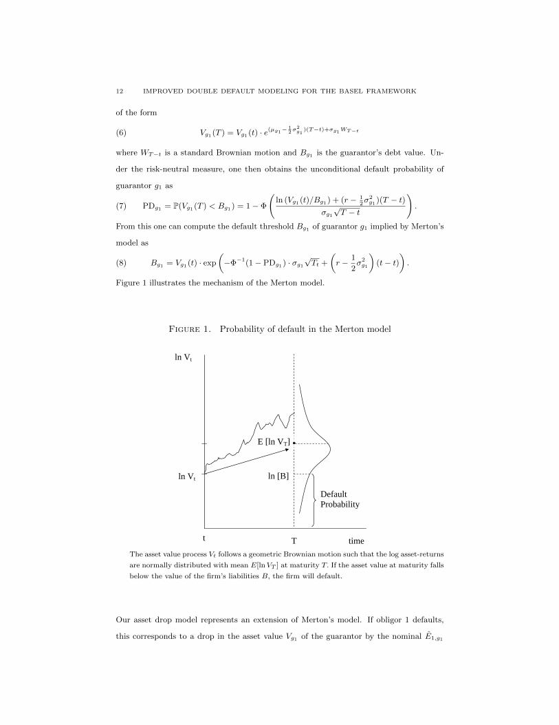
Figure 1 illustrates the mechanism of the Merton model.

Figure 1. Probability of default in the Merton model

E [ln VT]

ln Vt ln [B]

Default Probability

ln Vt

t T time

The asset value process Vt follows a geometric Brownian motion such that the log asset-returns

are normally distributed with mean E[lnVT ] at maturity T. If the asset value at maturity falls

below the value of the firm’s liabilities B, the firm will default.

Our asset drop model represents an extension of Merton’s model. If obligor 1 defaults,

this corresponds to a drop in the asset value Vg1 of the guarantor by the nominal E1,g1


that g1 guarantees for obligor 1.13 Hence we model the asset value process of the guarantor

g1 as

(9) Vg1(T ) = Vg1(t) · e(µg1− 1

2σ2g1

)(T−t)+σg1WT−t − E1,g1 · 1l{V1(T )≤B1}.

Thus our model represents a jump-diffusion model in the sense that the jump time is

determined by the stopping time 1l{V1(T )≤B1} i.e. by the default time of obligor 1 triggering

the guarantee payment. Moreover, the jump size is deterministic and given by the nominal

E1,g1 that g1 guarantees for obligor 1. We refer to this type of model as a Bernoulli mixture

model.14 The guarantor defaults with the increased probability PD′g1 when the guarantee

payment has been triggered, i.e. under the risk-neutral measure the increased default

probability of g1 is given by

(10)

PD′g1 = P (Vg1(T ) ≤ Bg1 |V1(T ) ≤ B1)

= P(Vg1(t) · e(r−

12σ2g1

)(T−t)+σg1WT−t − E1,g1

)= 1− Φ

ln(

Vg1 (t)

Bg1+E1,g1

)+(r − 1

2σ2g1

)(T − t)

σg1√T − t

.

Similarly the guarantor defaults with the probability PDg1 if obligor 1 survives, i.e.

(11)

PDg1 = P (Vg1(T ) ≤ Bg1 |V1(T ) ≥ B1)

= P(Vg1(t) · e(r−

12σ2g1

)(T−t)+σg1WT−t

)= 1− Φ

(ln (Vg1(t)/Bg1) +

(r − 1

2σ2g1

)(T − t)

σg1√T − t

).

Figure 2 illustrates the functioning of our new asset drop approach. In particular, it shows

how the guarantor PD increases when the guarantee payment has been triggered.

Note that Bg1 is the default threshold of guarantor g1 in case the hedged obligor 1 has

not defaulted. Thus Bg1 can be computed from the guarantor’s observed rating according

to the classical Merton model by equation (8). Thus, we can compute the increased PD′g1

of the guarantor due to the obligor’s default using equations (8) and (10). This then

13Note that at this point it can be seen that the model is, in principle, capable to capture also

other dependencies such as business-to-business relationships. For example, if it is known thatthe guarantor also has a direct claim of E1,g1 to obligor 1, it might be reasonable to continue

the computation with the higher asset drop E1,g1 +E1,g1 . To appropriately treat risky collaterals

E1,g1 could be taken as expected exposure at default.14Note that a classical jump diffusion model as e.g. in Zhou (2001b) is not suitable to model

double default effects for the following reason. In the jump-diffusion model of Zhou (2001b) the

jumps are driven by a Poisson process with intensity λ and the jump amplitude is stochastic aswell. The main idea of our double default model is that we model explicitly the time when the

asset value drops (resp. jumps) by considering the default time of the obligor that is hedged.This then leads to a Bernoulli-mixture model as stated above. Moreover, in our setting the jump

amplitude is deterministic as the amount that is guaranteed should be known in advance.


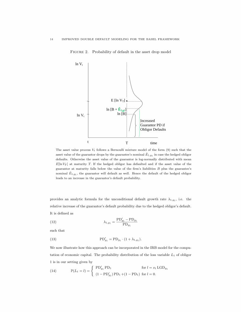
Figure 2. Probability of default in the asset drop model

E [ln VT]

ln Vt Increased Guarantor PD if Obligor Defaults

ln [B + Ê1,g1]ln [B]

ln Vt

t T time

The asset value process Vt follows a Bernoulli mixture model of the form (9) such that the

asset value of the guarantor drops by the guarantee’s nominal E1,g1 in case the hedged obligor

defaults. Otherwise the asset value of the guarantor is log-normally distributed with mean

E[lnVT ] at maturity T. If the hedged obligor has defaulted and if the asset value of the

guarantor at maturity falls below the value of the firm’s liabilities B plus the guarantee’s

nominal E1,g1 , the guarantor will default as well. Hence the default of the hedged obligor

leads to an increase in the guarantor’s default probability.

provides an analytic formula for the unconditional default growth rate λ1,g1 , i.e. the

relative increase of the guarantor’s default probability due to the hedged obligor’s default.

It is defined as

(12) λ1,g1 =PD′g1 −PDg1

PDg1

such that

(13) PD′g1 = PDg1 · (1 + λ1,g1).

We now illustrate how this approach can be incorporated in the IRB model for the compu-

tation of economic capital. The probability distribution of the loss variable L1 of obligor

1 is in our setting given by

(14) P(L1 = l) =

{PD′g1 PD1 for l = s1 LGDg1

(1− PD′g1) PD1 +(1− PD1) for l = 0.


Note that to respect double recovery effects LGDg1 could be multiplied by LGD1 . How-

ever, for several reasons double recovery is not reflected in the current Basel II frame-

work. Thus in the above and in the following we always set LGD1 = 1 such that

only recovery of the guarantor is accounted for. Then the expected loss for obligor 1

is E[L1] = s1 LGDg1 PD1 PD′g1 and the expected loss conditional on a realization xq of

the systematic risk factor X is

E[L1|xq] = s1 LGDg1 PD1(xq) PD′g1(xq)

where the conditional PDs are computed as in the IRB approach by

PD1(X) = Φ

(Φ−1(PD1)−√ρ1X√

1− ρ1

)and respectively for PD′g1 . Hence the unexpected loss capital requirement K1 for the

hedged exposure s1 is15

K1 = LGDg1(PD1(xq) PD′g1(xq)− PD1 PD′g1).

Hence, to compute the IRB capital charges for the hedged exposure to obligor 1, one

simply inserts the double default probability PD′g1 PD1 instead of PD1 in the formula for

the IRB risk weight functions.

Remark 3. (Convexity of effective guarantor PD) By taking derivatives in equations (8)

and (10) it can be shown that PD′g is convex in the guarantee nominal. This convexity sets

an incentive for banks to use several distinct guarantors for various loans. If, for example,

there are two identical loans and two guarantors with exactly the same characteristics,

the overall increase in default probability is smaller if each guarantor is contracted for

one of the loans compared to when one guarantor is chosen to guarantee both loans.

Thus also the bank’s economic capital will be smaller if it diversifies its guarantor risk.

In particular, as will be shown explicitly in Example 1, overly excessive contracting of

the same guarantor will significantly increase economic capital. This definitely is an

appreciated consequence from a regulatory point of view. However, the effect is not

reflected in the current treatment of double default effects within the IRB approach.

Under this approach economic capital does not depend on whether a hundred loans are

hedged by one single guarantor or whether every loan is hedged by one out of a hundred

different guarantors.

15The Basel II economic capital for the hedged exposure 1 is obtained by multiplying K1 with

the scaling factor 1.06 and the maturity adjustment MA1, where we insert PD1 PD′g1 instead ofPD1 .


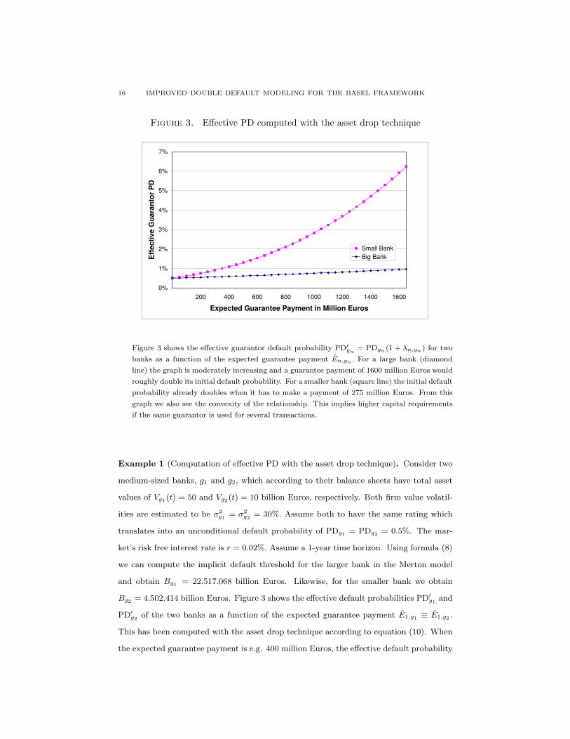
Figure 3. Effective PD computed with the asset drop technique

0%

1%

2%

3%

4%

5%

6%

7%

200 400 600 800 1000 1200 1400 1600

Expected Guarantee Payment in Million Euros

Eff

ec

tiv

e G

ua

ran

tor

PD

Small Bank

Big Bank

Figure 3 shows the effective guarantor default probability PD′gn = PDgn (1 + λn,gn ) for two

banks as a function of the expected guarantee payment En,gn . For a large bank (diamond

line) the graph is moderately increasing and a guarantee payment of 1600 million Euros would

roughly double its initial default probability. For a smaller bank (square line) the initial default

probability already doubles when it has to make a payment of 275 million Euros. From this

graph we also see the convexity of the relationship. This implies higher capital requirements

if the same guarantor is used for several transactions.

Example 1 (Computation of effective PD with the asset drop technique). Consider two

medium-sized banks, g1 and g2, which according to their balance sheets have total asset

values of Vg1(t) = 50 and Vg2(t) = 10 billion Euros, respectively. Both firm value volatil-

ities are estimated to be σ2g1 = σ2

g2 = 30%. Assume both to have the same rating which

translates into an unconditional default probability of PDg1 = PDg2 = 0.5%. The mar-

ket’s risk free interest rate is r = 0.02%. Assume a 1-year time horizon. Using formula (8)

we can compute the implicit default threshold for the larger bank in the Merton model

and obtain Bg1 = 22.517.068 billion Euros. Likewise, for the smaller bank we obtain

Bg2 = 4.502.414 billion Euros. Figure 3 shows the effective default probabilities PD′g1 and

PD′g2 of the two banks as a function of the expected guarantee payment E1,g1 ≡ E1,g2 .

This has been computed with the asset drop technique according to equation (10). When

the expected guarantee payment is e.g. 400 million Euros, the effective default probability


of the smaller bank would be PD′g2 = 1.09%, which corresponds to an increase by a factor

(1 + λ1,g2) = 2.19, i.e. λ1,g2 = 1.19. This means, that a financial institution which has no

direct exposure to g2 and which buys protection from the latter for its 400 million expo-

sure to obligor 1, will use this increased default probability when computing its economic

capital due to obligor 1. This is intuitive as g2’s default is only of interest when obligor 1

already has defaulted. For the larger bank the guarantee payment corresponds to a less

significant loss. Its effective PD would only increase by a factor (1 + λ1,g1) = 1.18 to

PD′g1 = 0.59%.

Note also that the relationship is convex as already mentioned in Remark 3. Also note

from equations (8) and (10) that the increase in PD is scale invariant with respect to the

firm size and the loan nominal. Thus, for example, a true global player with 100 times

the firm size of the large bank considered here could guarantee 100 times as much as the

large bank while suffering from the same increase in PD .

3.2. Generalizations. Let us now consider the more complicated case where there is

direct exposure to the guarantor. Denote the exposure share of obligor 1 by s1 and

assume that it is fully hedged by guarantor g1. Denote the direct exposure share to the

guarantor by sg1 . In this case we also have to focus on the default of the guarantor itself,

i.e. a loss also occurs if the guarantor defaults and the hedged obligor survives. In this

situation, in a sense, there are two appropriate default probabilities of the guarantor. If

obligor 1 already has defaulted, the default probability of the guarantor is given by PD′g1 .

Otherwise it is given by PDg1 . To compute the contribution to economic capital of the

hedged obligor and its guarantor within in the IRB approach we have to compute the

conditional expected loss of both. As we do not want to reflect double recovery effects

(similarly to the treatment in Basel II) we set LGD1 = 1 for a hedged exposure. The

probability distribution of the joint loss variable L1,g1 of obligor 1 and its guarantor g1,

is then

(15) P(L1,g1 = l) =

PD′g1 PD1 for l = s1 LGDg1

+sg1 LGDg1

PDg1(1− PD1) for l = sg1 LGDg1

(1− PD′g1) PD1 +(1− PDg1)(1− PD1) for l = 0.

Note that the increased unconditional default probability PD′g1 occurs together with

PD1 (i.e. with the probability that obligor 1 defaults), as in these situations the guarantee

payment is triggered. The first case corresponds to the situation where both the obligor


and the guarantor default (i.e. to the double default case). In the second case only the

guarantor defaults such that only the direct exposure to g1 is lost. The third case comprises

the hedging case, i.e. the obligor defaults and the guarantor succeeds in delivering the

guarantee payment (although its default probability has increased) and the case where

both the guarantor and the obligor survive. Thus in this case no loss occurs. The expected

loss can be computed as

E[L1,g1 ] = PD′g1 PD1(sg1 LGDg1 +s1 LGDg1)

+ PDg1(1− PD1)sg1 LGDg1

= sg1 LGDg1

(PDg1 + PD1 ·(PD′g1 −PDg1)

)+s1 LGDg1 PD′g1 PD1

This can be reformulated as

(16) E[L1,g1 ] = sg1 LGDg1 PDg1(1 + λ1,g1 PD1) + s1 LGDg1 PD′g1 PD1 .

Note that probability that the exposure sg1 in the first term is lost, is the expected default

probability of the guarantor whereas the probability that the hedged exposure s1 in the

second term is lost, is the default probability of the guarantor conditional on obligor 1’s

default. The second term in equation (16) is the expected loss due to obligor 1 that only

occurs in the situation of double default. This term is the same as in the case where the

guarantor is external. The first term in equation (16) is the expected loss due to obligor 2

whose default probability increases if it has to exercise its guarantee payment. That is,

the expected loss due to an obligor increases if it is involved in a hedging activity because

its expected PD increases. This fact is ignored in the treatment of double default effects

in the IRB approach since guarantors are implicitly treated as external.16

The derivation of economic capital for the hedged exposure and its guarantor is obtained

as follows. The conditional expected loss can be obtained as in the model underlying the

IRB treatment of double default effects when there is no additional correlation. Denote by

rn resp. rgn the log asset return of obligor n resp. of its guarantor gn. Let the conditional

default probabilities be defined as in the IRB model by

(17) PDn(X) = Φ

(Φ−1(PDn)−√ρnX√

1− ρn

)

16Note, again, that under the IRB approach it would not be reasonable to take into account directexposure to a guarantor as the additional correlation would induce an unrealistic dependency

between obligor and guarantor.


for n = 1 or g1 and analogously for PD′g1(X). Then in our setting we have

(18)

E[L1,g1 |X] = s1 LGDg1 E[1l{r1<c1}1l{rg1<c′g1}|X]

+sg1 LGDg1 E[1l{rg1<cg1}1l{r1≥c1} + 1l{rg1<c′g1}1l{r1<c1}|X]

= s1 LGDg1 PD1(X) PD′g1(X)

+sg1 LGDg1

(PDg1(X)(1− PD1(X)) + PD′g1(X) PD1(X)

)where we again neglected double recovery effects. Note that the loss variables for s1 and sg1

in the above equation are stochastically dependent conditional on X. Thus, approximating

the value-at-risk αq(L) by the conditional expected portfolio loss as it is done in the IRB

approach only makes sense within a double default treatment when the hedged exposure

shares and the direct exposure shares to guarantors are sufficiently small (compare Remark

1 for more details).

Partial hedging and the case where a guarantor hedges multiple obligors in a portfolio can

be approached with the same technique just presented and the results are straightforward.

See also Ebert and Lutkebohmert (forthcoming) for a detailed treatment of these situations

under Pillar 2 of Basel II.

Example 2. (Comparison of EC computed with the IRB double default treatment and

with the asset drop technique.) Consider a portfolio with N = 110 obligors. The first

n = 1, . . . , 10 loans in the portfolio are hedged by guarantors 101, . . . , 110, who also act

as obligors in the portfolio. Assume the exposures to equal EADn = 1 for all n =

1, . . . , 110. The PDs are assumed to be 1% for n = 1, . . . , 100 and 0.1% for the guarantors

n = 101, . . . , 110. As in the IRB approach, let LGDs be 45% for all unhedged obligors

n = 11, . . . , 110. Hedged exposures are assigned an LGD of 100% to neglect double recovery

effects, i.e. LGDn = 100% for n = 1, . . . , 10. We assume an effective maturity of M = 1

year for all obligors and guarantors in the portfolio. Value-at-risk is computed at the

99.9% percentile level. The IRB treatment of double default effects yields an economic

capital of 5.40% of total exposure.17 This is lower than the value obtained when neglecting

double default effects entirely which equals 5.79%. Denoting by xq the qth percentile of

the systematic risk factor X, we calculated the IRB capital with the asset drop technique

17This computation is based on the approximation in equation (1) as this is the one applied inpractice.


as

(19)

10∑n=1

sn LGDgn

[PDn(xq)PD

′gn(xq))− PDn PDgn(1 + λn,gn)

]+

100∑n=11

sn LGDn (PDn(xq)− PDn)

+

110∑n=101

sgn LGDgn

[PDgn(xq) · (1− PDn(xq)) + PD′gn(xq) PDn(xq)

−PDgn(1 + PDn ·λn,gn)].

In the above equation PD′gn(xq) denotes the conditional increased default probability for

the guarantor computed via equation (17) with PD equal to PDgn(1 + λn,gn) and asset

correlation parameter ρ set to 0.7. The latter value is the increased correlation parameter

chosen in the IRB treatment for exposures subject to double default. Although the choice

of this parameter might be questionable we use it here for reasons of better comparability

of our model with the IRB treatment of double defaults.

Figure 4. Influence of increased guarantor PD on EC

5,3

5,4

5,5

5,6

0,1 0,2 0,3 0,4 0,5 0,6

(Increased) guarantor PD

EC

in

perc

en

tag

e o

f

to

tal

exp

osu

re

Figure 4 shows the influence of the parameter λ through the increased guarantor default

probability PD′gn = PDgn (1 + λn,gn ) on regulatory capital computed within the asset drop

model. λ increases from 0.0 to 5.0 leading to an increase in EC from 5.34% to 5.61% of total

portfolio exposure. For λ = 0.7 (PD′gn = 0.17%) the asset drop model leads to the same

EC = 5.40% as the IRB treatment of double defaults.

Figure 4 shows the influence of the parameter λ through the increased default probability

PD′gn = PDgn(1 +λ) of the guarantor on the IRB capital computed within the asset drop

approach. Here we chose a constant level of λ for all hedged obligors in the portfolio.


With increasing λ the IRB capital also increases. This is very intuitive as higher values of

λ mean that the expected default probabilities of the guarantors increase. This obviously

results in higher capital requirements. For λ = 0.7 (PD′gn = 0.17%) our new asset drop

method leads to the same economic capital as the one computed within the IRB treatment

of double defaults, i.e. EC = 5.40% of total portfolio exposure.

4. Conclusion

In this paper we pointed out several severe problems of the treatment of double default

effects applied under Pillar 1 in the Basel framework’s IRB approach. Our main criticism

is that it relies on the assumption of additional correlation between obligors and guaran-

tors. Thus, it fails to model their asymmetric dependence structure appropriately, that

is, that the guarantor should suffer much more from the obligor’s default triggering the

guarantee payment than vice versa. The particular choice for the additional correlation

parameter is the same for all obligors and guarantors and it remains entirely unclear how

specific guarantor and obligor characteristics could be reflected in this parameter. Further,

all guarantors are treated as distinct for different obligors and are assumed to be external

to the portfolio. Thus, if there is direct exposure to guarantors or if several obligors have

the same guarantor, then the additional dependencies and concentrations in the credit

portfolio are ignored. Hence, also overly excessive contracting of the same guarantor is

not reflected in the computation of economic capital.

To overcome these deficiencies, we proposed a new approach to account for double default

effects that can be applied in any model of portfolio credit risk and, in particular, under

the IRB approach. It is easily applicable in terms of data requirements and computational

time. Specifically, compared to the model of Heitfield and Barger (2003) underlying the

IRB treatment of double defaults we need in addition the total values of the firms’ assets.

These, however, can be directly inferred from the balance sheets and hence it should not

be too much of a burden for any bank. Moreover, it should be obvious that theses quan-

tities should be reflected in any good model for double default effects.

Despite of its simplicity our new approach does not show any of the above mentioned

shortcomings and thus better reflects the risk associated with double defaults. The model

endogenously quantifies the impact of the guarantee payment on the guarantor’s uncondi-

tional default probability. Within a structural model of portfolio credit risk the guarantor’s


loss due to the guarantee payment corresponds to a downward jump in its firm value pro-

cess. The jump size is determined endogenously through the underlying credit risk model

assumed. This new asset drop technique could also be applied to model other dependen-

cies within a conditional independence framework, as for example default contagion effects

through business-to-business dependencies.

References

Basel Committee on Banking Supervision, 2003. Basel II: International convergence of

capital measurement and capital standards: a revised framework. Bank for International

Settlements.

Basel Committee on Banking Supervision, 2005. The application of Basel II to trading ac-

tivities and the treatment of double default effects. Bank for International Settlements.

Basel Committee on Banking Supervision, 2006. Basel II: international convergence of

capital measurement and capital standards: a revised framework. Publication No. 128.

Bank for International Settlements.

Basel Committee on Banking Supervision, 2009. Strengthening the resilience of the bank-

ing sector. Consultative Document. Bank for International Settlements.

Brigo, D., Chourdakis, K., 2009. Counterparty risk for credit default swaps. International

Journal of Theoretical and Applied Finance 12 (7), 1007–1026.

Ebert, S., Lutkebohmert, E., forthcoming. Treatment of double default effects within the

granularity adjustment for Basel II. Journal of Credit Risk.

Gordy, M., 2003. A risk-factor model foundation for ratings-based bank capital rules.

Journal of Financial Intermediation 12 (3), 199–232.

Gregory, J., 2009. Being two-faced over counterparty credit risk. Risk Magazine 22 (2),

86–90.

Grundke, P., 2008. Regulatory treatment of the double default effect under the New Basel

Accord: how conservative is it? Review of Managerial Science 2, 37–59.

Heitfield, E., Barger, N., 2003. Treatment of double-default and double-recovery effects

for hedged exposures under Pillar I of the proposed New Basel Accord, White Paper

by the Staff of the Board of Governors of the Federal Reserve System.

Hull, J., White, A., 2001. Valuing credit default swaps II: modeling default correlations.

Journal of Derivatives 8 (3), 12–22.


Leung, S., Kwok, Y., 2005. Credit default swap valuation with counterparty risk. The

Kyoto Economic Review 74 (1), 25–45.

Lipton, A., Sepp, A., 2009. Credit value adjustment for credit default swaps via the

structural default model. The Journal of Credit Risk 5 (2), 127–150.

Merton, R., 1974. On the pricing of corporate debt: the risk structure of interest rates.

Journal of Finance 29, 449–470.

Pykhtin, M., 2010. Modeling credit exposure for collateralized counterparties. The Journal

of Credit Risk 5 (4), 3–27.

Pykhtin, M., Zhu, S., 2007. A guide to modelling counterparty credit risk. GARP Risk

Review July/ August, 16–22.

Taplin, R., To, H., Hee, J., 2007. Modeling exposure at default, credit conversion factors

and the Basel II accord. Journal of Credit Risk 3 (2), 75–84.

Valvonis, V., 2008. Estimating EAD for retail exposures for Basel II purposes. Journal of

Credit Risk 4 (1), 79–101.

Zhou, C., 2001a. An analysis of default correlations and multiple defaults. Review of

Financial Studies 14 (2), 555–576.

Zhou, C., 2001b. The term structure of credit spreads with jump risk. Journal of Banking

and Finance 25, 2015–2040.

improved double default modeling for the basel framework ... · improved double default modeling...

Documents