improved estimation of reserves in gas condensate …

IJRRAS 43 (1) ● April-June 2020 www.arpapress.com/Volumes/Vol43Issue1/IJRRAS_43_1_03.pdf

20

IMPROVED ESTIMATION OF RESERVES IN GAS CONDENSATE

RESERVOIRS

Joseph James Olushola and Sunday Isehunwa

The University of Ibadan, Ibadan, Oyo State, Nigeria

ABSTRACT

Estimating Gas condensate reserves and predicting their performance has been an area to reconcile with in the

industry today. The general method of estimating the volume of gas (reserves) in a gas reservoir is the Gas Material

Balance (P/Z against Gp plot). This method basically involves computing gas compressibility factors (z) at different

pressures during production from the reservoir. Condensate reservoirs exhibit two phase occurrence as reservoir

pressure is depleted below dew point, hence posing a challenge to accurately estimating the compressibility factor (z

factor) to be used for the plot. This may ultimately result in underestimating or overestimating the Gas-Initially-In-

Place in such reservoirs. The reservoir fluid acquired from the field is used in experimental Constant Volume

Depletion simulation to acquire data representing the actual reservoir depletion which is validated with observed

minimal deviations and presented in the PVT reports. To replace the need for time consuming and complicated

experiments, it was attempted to develop a relationship or model to determine the best estimates of the two-phase

compressibility factors at different pressures. In this paper, the Peng-Robinson's equation of state is employed to

determine the different phase compressibility factors and combined in proportions with respect to the overall mole

fractions of the two phases as a weighting factor to obtain a general relationship for the two-phase compressibility

factor of the reservoir fluid. The reserve estimates from this method were compared with the field data and other

methods for possible deviations and corrections. It is conclusive that this project results in the highest accuracy in

condensate reserves estimation with an average error of about 1%, whereas obtainable error using the Standing-Katz

single phase z factor could be up to 8%.

Keywords: Two Phase Z factor, Peng-Robinson EOS, CVD simulation, P/Z plot, Standing Katz, z factor

1. INTRODUCTION

Gas condensate reservoirs are characterized by production of both surface gas and varying quantities of stock-tank

oil (STO). The STO is commonly referred to as "condensate" or "distillate". Typical condensate surface yields range

from 10 to 300 STB/MMscf. The added economic value of produced condensate in addition to gas production

makes the recovery of condensate a key consideration in developing gas condensate reservoirs; in the extreme case

of a non-existent gas market, producible condensate is the only potential source of income.

At reservoir conditions, a gas condensate reservoir contains single phase gas. The gas flows from the reservoir

through the production tubing to the surface separator, and then liquid condenses from the gas. Isothermal

condensation of liquids in the reservoir as pressure drops below the dew point pressure constitutes the process of

retrograde condensation. Liquids condensed in the reservoir are mostly lost or unrecoverable. In a gas-condensate

reservoir, the initial reservoir condition is in the single phase area to the right of the critical point. As the reservoir

pressure declines, the fluid passes through the dew point and a liquid drops out of the gas, the percentage of vapour

decreases, but can increase again with continued pressure decline.

A main difference between a "gas" reservoir and a "gas condensate" reservoir is that a gas reservoir will not

experience two hydrocarbon phases at reservoir conditions, and hence there will be no liquid condensation

("condensate loss") in the reservoir.

Furthermore, a gas reservoir would not have significant condensable surface liquids to "loose" due to retrograde

condensation. This leads to the apparent contradiction that the leaner the gas condensate, the higher the condensate

recovery (as a percentage of initial in place). Surface separators typically operate at conditions of low pressure and

low temperature. [1]

Another important difference between gas and gas condensate reservoirs is the loss in well deliverability

experienced by gas condensate reservoirs due to the buildup of significant liquid saturations near the wellbore. Gas

reservoirs will not experience such deliverability loss because liquids do not condense at reservoir temperature.

IJRRAS 43 (1) ● April-June 2020 Olushola & Isehunwa ● Improved Estimation of Reserves in Gas

21

2. PROBLEM FORMULATION

Condensate reservoirs exhibit two phase phenomenon at pressures below the dew point and this affects the

qualitative parameters used in characterizing the fluid system (i.e. z factor considered in this project). Therefore, it is

necessary to convert the single-phase parameters to a usable one for two phase system.

Calculations of initial gas and condensate in place require the use of the real gas equation of state, with some

modifications.

First, we calculate volumetrically the volume of gas condensate per volume of reservoir:

R

R

zRT

VPG

4.379= (1)

There are two basic cases of every condensate system with respect to the dew point pressure; i.e. when the reservoir

pressure is above the dew point pressure (when the system is strictly single gas phase) and when the pressure below

the dew point.

Case I - Reservoir Pressure above Dew point Pressure

The p/z vs. Gp form of the material balance is also used for gas condensate reservoirs when reservoir pressure is

above the dew point. The cumulative gas production is modified to include the condensate production. This gas is

called "wet" gas. The volume of condensate produced is converted to its gas equivalent (GE) by assuming that the

condensate can be expressed in terms of an ideal gas,

SC

SC

O

Op

SC

SC

P

RT

M

Na

P

nRTVGE

2=== (2)

In summary, the material balance for a volumetric gas condensate reservoir above the dew point is,

−=

W

PW

i

i

G

G

z

P

z

P1 (3)

Where, Gw is initial wet gas in place, and Gpw produced wet gas.

Case II - Reservoir Pressure below Dew point Pressure

When the reservoir pressure drops below the dew point pressure, condensate drops out of the reservoir gas. This

violates several of the basic assumptions implicit in the traditional gas material balance equation.

One of the earlier solutions to this problem was the Constant Volume Depletion experiment - a laboratory

experiment designed to duplicate or model closely the reservoir depletion of a volumetric gas condensate reservoir,

the experiment is a constant volume depletion experiment (CVD).

The standard experimental program for the analysis of a gas-condensate fluid includes

(1) Recombined wellstream compositional analysis through C7+

(2) Constant composition expansion (CCE), and

(3) Constant volume depletion (CVD).

The CCE and CVD data are measured in a high-pressure visual cell where the dew point pressure is determined

visually. Total volume/pressure and liquid-dropout behaviour is measured in the CCE experiment.

The CCE data for a gas condensate usually include total relative volume, Vrt, defined as the volume of gas or of gas-

plus-oil mixture divided by the dew point volume. Z factors are reported at pressures greater than and equal to the

dew point pressure. With relevance to this study they could be used to determine dew point z factor, Zd of the

condensate fluid system.

Phase volumes defining retrograde behaviour are measured in the CVD experiment together with Z factors and

produced-gas compositions through C7+. Optionally, a multistage separator test can be performed as well as TBP

analysis or simulated distillation of the C7 into single-carbon-number cuts from C7 to about C20+.


22

Knowing the cumulative moles removed and its volume occupied as a single-phase gas at the removal pressure, we

can calculate the equilibrium gas Z factor from

RTn

VPz

g

g

= (4)

The CVD experiment provides data that can be used directly by the reservoir engineer. From the data obtained, a

“two-phase” Z factor is also reported. This is calculated assuming that the gas-condensate reservoir depletes

according to the material balance for a dry gas and that the initial condition of the reservoir is at dew point pressure

Where Gpw = cumulative wellstream (wet gas) produced and Gw = Initial wet gas in place.

It is defined that the term Gpw/Gw equals np/n reported in the CVD report. From Eq. 3, the only unknown at a given

pressure is Z2, and the two-phase Z factor is then given by

−

=

n

nzP

Pz

Pdd 1

2 (5)

3. SCOPE OF STUDY

This study is based on the Gas MBE application using Peng-Robinson equation of state (PREOS) derived two phase

z factors and using existing data for liquid and vapour phase compositions (from flash) and CVD z factors in the

PVT Reports by Flo-petrol for OBEN Field wet gases with appreciable amount of wet gas and condensate recovery.

Objectives

The objective of this project is to accurately or near accurately determine the amount of Gas Initially in Place (GIIP)

in gas condensate reservoirs. In achieving this, the project focuses on the use of simple systematic and linear model

by using overall mole fractions as a weighting factor. The project also applies Fortan and Matlab programs to

automate the generation of z factor and simplify the calculations..

4. METHODOLOGY

4.1 Introduction

In this study, a novel mathematical-based approach is proposed to develop reliable model for prediction

of compressibility factor of natural gas condensate using the Peng Robinson equation of state [2] based on Slot-

Petersen [3] binary interaction parameters and adopting some principles from the Zudkevitch and Joffe’s [4]

approach to solving the Redlich Kwong EOS.

P/Z = (P/Zi)i[1 – Gp/G]

Z2ph = ZvV + ZLL (6)

The Peng-Robinson equation was developed in 1976 at The University of Alberta in order to satisfy the following

goals:

• The parameters should be expressible in terms of the critical properties and the acentric factor.

• The model should provide reasonable accuracy near the critical point, particularly for calculations of the

compressibility factor and liquid density.

• The mixing rules should not employ more than a single binary interaction parameter, which should be

independent of temperature pressure and composition.

• The equation should be applicable to all calculations of all fluid properties in natural gas processes.

To generate the required estimates for compressibility factors, it would involve;

• Solving the equations for two phase hydrocarbon fluids incorporating the flash calculations

• Solving the PREOS and the required binary interaction coefficients


23

• Defining and correlating the fugacity –and fugacity coefficient equations

• Accounting for the effects of the heavy hydrocarbon plus fractions on the phase equilibra predictions

4.2 The Peng-Robinson Equation of State for Mixtures

As written, the P-R equation is intended for description of the PVT behaviour of pure compounds.

However, it can also be used for mixtures of compounds by using "mixture-averaged" values for the equation

parameters, as adopted from Ahmed T. [5-7].

)()(

)(

bVbbVV

Ta

bV

RTP

−++−

−=

(7)

Here, R is the gas constant, P is the absolute pressure, T is the absolute temperature, v is the molar volume, and b

and a(T) are given by:

(8)

(9)

(10)

(11)

Here, Tc is the critical (absolute) temperature, Pc is the critical (absolute) pressure, and is the Pitzer acentric

factor. Thus the P-R equation has in effect just three compound-specific experimentally-determined physical

properties: Tc , Pc , and .

Note that if the compressibility factor z =Pv /(RT), then (1) can be written as a cubic equation in z :

z3 - (1 - B)z2 + (A - 3B2 - 2B)z - (AB - B2 - B3) = 0

Here, B = Pb/(RT) and A = aP/(RT)2.

Let the values of parameters aii(T) and bi be the pure-component values of a(T) and b, respectively, for the i(th)

compound in a mixture.

Also, let xi be the mole fraction of component i in the vapour phase of the mixture.

Then "mixing" rules are applied to compute the mixture-averaged values of a(T) and b for a mixture of n different

compounds as follows:

=

=n

i

iim bxTb1

)( (12)

)1( ijjijijim kaaxxa −= (13)

Where Kij is the binary interaction parameter

The corresponding values of a and b for the liquid phase will be obtained by replacing x with yi ie, mole the mole

fraction of component i in the liquid phase of the mixture

NB: It is to be noted that Equations of States (EOS) are not perfect;

EOS provides self-consistent fluid properties;

2

2/1

22

26992.054226.137464.0

)1(1)]([

07780.0)(

)(45724.0)(

−+=

−+=

=

=

m

T

TmT

P

RTTb

TP

TRTa

C

C

C

C

C


24

• Density (oil or gas) trends are correctly predicted with pressure, temperature, and compositions (and all

derived properties).

• Same phase equilibrium model for gas and liquid phases (material balance consistency).

However, predicted fluid property values may differ substantially from data. EOS are routinely “calibrated” to

selected & limited experimental data, After “calibration” EOS predictions beyond range of data can be used with

confidence, and EOS are extensively used in reservoir simulation.

4.3 Equation of State (EOS) calibration

Minimization of squared differences between experimental and predicted fluid properties

( ) min

2

1

)(exp)( =−=

N

i

erimentalipredictedi gg

(14)

These Properties (gi) include:

• Densities, saturation pressures, Relative amounts of gas and liquid phases Compositions, etc.

• Accomplished by changing within certain limits selected EOS parameters.

• Minor adjustments (1 to 2%) of binary interaction parameters (kij) can change saturation pressures by

20 to 30%

• Different properties of the C7+fraction affect liquid dropout and densities. These properties include;

1. Molecular weight (uncertainty is +/-10%)

2. Specific gravity

3. Critical properties and acentric factors which are highly dependent on correlations and cannot

be easily measured.

4.4. Binary Interaction Parameter

The parameter kij is an empirically determined correction factor (called the binary interaction coefficient) that is

designed to characterize any binary system formed by component i and component j in the hydrocarbon mixture.

These binary interaction coefficients are used to model the intermolecular interaction through empirical adjustment

of the (aα)m term as represented mathematically.

They are dependent on the difference in molecular size of components in a binary system and they are characterized

by the following properties:

• The interaction between hydrocarbon components increases as the relative difference between their

molecular weights increases: ki,j+1 > ki,j

• Hydrocarbon components with the same molecular weight have a binary interaction coefficient of zero:

ki,i = 0

• The binary interaction coefficient matrix is symmetric: kj,i = ki,j

Slot-Petersen (1987) [3] and Vidal and Daubert (1978) [8] presented a theoretical background to the meaning of the

interaction coefficient and techniques for determining their values. Graboski and Daubert (1978) [9] and Soave

(1972) [10] suggested that no binary interaction coefficients are required for hydrocarbon systems.

To provide the modified PR EOS with a consistent procedure for determining the binary interaction coefficient kij,

the following computational steps are proposed:

Step 1. Calculate the binary interaction coefficient between methane and the heptanes-plus fraction from:

kc1-c7+ = 0 00189T- 1 167059

where the temperature T is in °R.

Step 2. Set: kCO2–N2 = 0.12

kCO2-hydrocarbon = 0.10


25

kN2- hydrocarbon = 0.10

Step 3. Adopting the procedure recommended by Petersen (1989)[11], calculate the binary interaction coefficients

between components heavier than methane (e.g., C2, C3) and the heptanes-plus fraction from:

kCn - c7+ =0.8 kc(n-1) - c7+

where n is the number of carbon atoms of component Cn;

e.g: Binary interaction coefficient between C2 and C7+ is kC2 – C7+ = 0.8 kC1 – C7+

Binary interaction coefficient between C3 and C7+ is kC3 – C7+ = 0.8 kC2 – C7+

Step 4. Determine the remaining kij from:

−

−=

+

+−)()(

)()(55

7

55

71

iC

ij

CCijMM

MMkk

(15)

where M is the molecular weight of any specified component.

For example, the binary interaction coefficient between propane C3 and butane C4 is:

−

−=

+

+−−)()(

)()(5

3

5

7

5

3

5

47343

CC

CCCCCC

MM

MMkk

(16)

4.5 Solving the Peng Robinson equation of state (step by step)

The liquid and vapour phase mole fractions xi, yi, and the binary interaction coefficient kij, are used to solve the PR-

EOS and determine the liquid phase ZL factor and the vapour phase zv factor. The binary interaction parameter is

such that every two components, either molecules of different substances (e.g. C1 and C4) or those of same

compound (e.g. C1 and C1) are all considered.

Therefore every multicomponent system results has kij existing in an n x n matrix order, where n is the number of

components i.e. for a two component system there exist a 2 x 2 matrix order for kij values including, k11, k12, k21 ,

and k22.

Take am and bm from (12) and (13)

B = Pbm/(RT) and A = amP/(RT)2

Same process is carried out for the liquid phase using the flashed fractional compositions (yi) and the values are

computed and then substituted into the general equation;

z3 - (1 - B)z2 + (A - 3B2 - 2B)z - (AB - B2 - B3) = 0

Using the Newton Raphson iterative method, solve the above Equation and obtain ZL and Zv, i.e., smallest and

largest roots respectively, for liquid and vapour phases.

4.6. Flash Calculations

Flash calculations are an integral part of all reservoir and process engineering calculations. They are required

whenever it is desirable to know the amounts (in moles) of hydrocarbon liquid and gas coexisting in a reservoir or a

vessel at a given pressure and temperature. These calculations are also performed to determine the composition of

the existing hydrocarbon phases.

Given the overall composition of a hydrocarbon system at a specified pressure and temperature, flash calculations

are performed to determine:

• Moles of the gas phase nv

• Moles of the liquid phase nL

• Composition of the liquid phase xi

• Composition of the gas phase yi

The computational steps for determining nL, nv, yi, and xi of a hydrocarbon mixture with a known overall

composition of zi and characterized by a set of equilibrium ratios Ki are summarized in the following steps:

Step 1. Calculation of nv: Equation can be solved for nv by using the Newton–Raphson iteration techniques.


26

In applying this iterative technique:

• Assume any arbitrary value of nv between 0 and 1, e.g. nv could be 0.5, nv = 0.5.

A good assumed value may be calculated from the following relationship, providing that the values of the

equilibrium ratios are accurate:

nv= A/(A-B)

(17)

−=i

ii KzA )1(

(18)

−=

i

iii KKzB )1(

(19)

• Evaluate the function f(nv) as given by Equation 3.26 using the assumed value of nv

• If the absolute value of the function f(nv) is smaller than a preset tolerance, e.g.,10–15, then the assumed

value of nv is the desired solution.

• If the absolute value of f(nv) is greater than the preset tolerance, then a new value of nv is calculated from

the following expression

)(/)()( vvvnv nfnfnn −=

(20)

Where

+−

−=

i iv

ii

vKn

Kznf

1)1(

)1()(

(21)

+−

−−=

i iv

ii

Kn

Kzf

2

2

)1)1((

)1(

(22)

where (nv)n is the new value of nv to be used for the next iteration.

• The above procedure is repeated with the new values of nv until convergence is achieved.

Step 2. Calculation of nL: Calculate the number of moles of the liquid phase from;

nL = 1− nv

(23)

Also;

Wilson’s Correlation [12] is sufficient in determining the K values at low pressures.

−+=

T

T

P

PK ci

i

ci

i 1)1(37.5exp

(24)

Whitson and Torp (1983) [13-14] reformulated Wilson’s equation to yield accurate results at higher pressures.

Wilson’s equation was modified by incorporating the convergence pressure into the correlation, to give:

−+

=

−

T

TA

P

P

P

PK ci

ici

A

k

cii 1)1(37.5exp

1

(25)

7.0

1

−=

k

ci

P

PA

(26)

where p = system pressure, psig

Pk = convergence pressure, psig

T = system temperature, °R

This project is provided with CVD data which are used to infer the mole fraction of the vapour phase and the liquid

phase thus: In the laboratory, the removed gas (well-stream) is brought to atmospheric conditions, where the amount

of surface gas and condensate are measured. Surface compositions yg and xo of the produced surface volumes from


27

the reservoir gas are measured, as are the volumes ∆Vo and ∆Vg , densities ρo and ρg and oil molecular weight Mo.

From these quantities, we can calculate the moles of gas removed, ∆ng. [15]

379

g

O

OOg

V

M

Vn

+

=

(27)

These data are reported as cumulative well-stream produced, ng, relative to the initial moles n.

( )=

=

k

jjg

k

gn

nn

n

1

1

(28)

Then, we have that;

1−

−

=

=

k

p

k

p

k

g

gn

n

n

n

n

nn

(29)

Where =gn vapour phase mole fraction (of the produced fluid in cvd).

The result here would then be furher iterated and modified to be used in the required relation.

5. RESULTS AND DISCUSSION

a. The calculated z factors from this project is to be compared with those obtained from conventional two

phase z factors from constant volume depletion and constant composition expansion experiments in the lab

and the deviation is observed.

b. The equations are programmed and automated to generate the two phase z factor values and maintain

accuracy.

c. The p/z plot is then observed and correlated with other sources of reserves estimates available and the

deviations are observed and adjusted.

d. It is worthy of note that setting the k as zero and using the exact values yield very slight difference in the

results for z factors of about a maximum 0.0001 tolerance

e. Inaccuracy of the k values in determining actual mole fraction of the phase reflects a notable deviation from

experimental values; also, since it is known that the vapour mole fraction is 1.000 at the dew point, z factor

here is calculated strictly by using z=PV/nRT for that initial point.

f. The estimation of reserves based on this method is comparing the estimates of GIIP based on two phase z

factors obtained from this project and those obtained from the standing –Katz chart based on the Hall-

Yarborough[16-17] empirical representation, and the two phase z factors for the limited Rayes et al

correlation[18]

g. This project have provided its result with a very reliable source of data from PVT experiments actually

performed to determine accurately the composition of the gas produced by flashing from several pressures,

when the composition in mole percent of all the component in their several phases are not correct this

process will yield erroneous results.

h. When the phase mole fractions (weighting factors) becomes difficult to estimate due to inaccuracy in K-

value calculations; the Vapour phase z-factor (Zv) is still a very good approximation of the Z-2phase in

order to conveniently estimate the reserves using the P/Z plot.


28

5.1 Results

5.1.1. CASE 1 (OBEN 25, BHT= 158oF)

Table 1: The Z-factor Results for OBEN 25

Pressure

(psig)

Z

(reporte

d)

Zv

(PREOS)

ZL

(PREOS)

V

(overall

vapour phase

mole fraction

corrected)

Ztwo-phase

(This project)

Z1ph (single-

phase from

the

Standing-

katz [19,20]

chart)

Z rayes

(Rayes

correlation

for 2 phase z

factor)

3700 0.848 0.848(set) - 1.000000 0.848000 0.806 0.781319

3587 0.844 0.849172 1.806350 0.994654 0.854289 0.796 0.771561

3397 0.835 0.839848 1.713030 0.994509 0.844642 0.780 0.755240

3117 0.826 0.828028 1.575190 0.997300 0.830045 0.759 0.731381

2844 0.821 0.819178 1.440420 0.997067 0.820975 0.741 0.708341

2550 0.820 0.813288 1.294850 0.986063 0.819981 0.729 0.683774

2254 0.823 0.811991 1.147800 0.968681 0.822508 0.726 0.659298

1966 0.832 0.815996 1.004220 0.916438 0.831724 0.733 0.635731

1691 0.844 0.825288 0.866626 0.548812 0.843939 0.750 0.613456

1426 0.860 0.839634 0.733545 0.862754 0.824919 0.776 0.592202

1091 0.887 0.865371 0.564571 0.937135 0.846461 0.820 0.56563

601 0.933 0.916960 0.315777 0.933024 0.901732 0.895 0.527359

0 1.000 0.997837 0.872266 0.983349 0.995746 0.990 0.500000

Percentage Error in reserves estimation (referenced to report)

At (P/Z) dimensionless = 0.00

For This project =|(𝐺𝑝 𝐺⁄ )𝑐𝑎𝑙𝑐𝑢𝑙𝑎𝑡𝑒𝑑−(𝐺𝑝 𝐺⁄ )𝑐𝑜𝑟𝑟𝑒𝑐𝑡

(𝐺𝑝 𝐺⁄ )𝑐𝑜𝑟𝑟𝑒𝑐𝑡| × 100% = |

0.9954−1

1|=0.46%

For Single phase Z =|1.01895−1

1|=1.9%

For Rayes correlation =|1.138−1

1|=13.8%


29

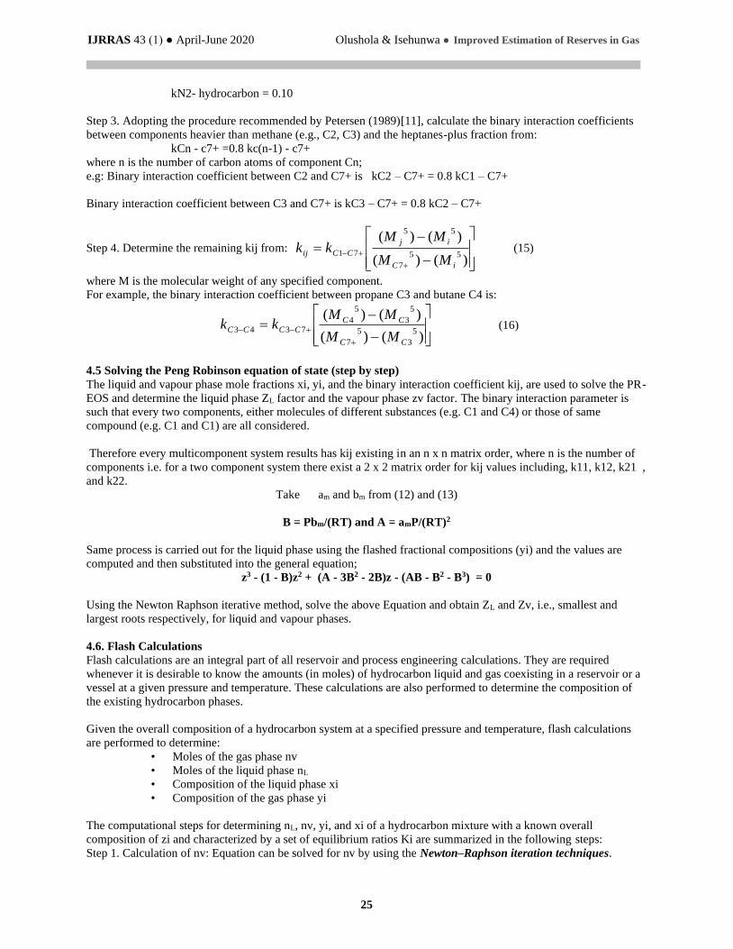
Fig.1. Z factor against Pressure OBEN 25

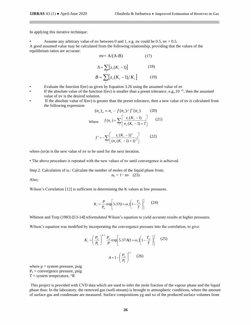
Fig.2. P/Z against against Gp Plot (DIMENSIONLESS FORM) OBEN 25


30

5.1.2. CASE 2 (OBEN 23, BHT= 143oF)

Table 2: The Z-factor Results for OBEN 23

Pressure

(psig)

Z

(reporte

d)

Zv

(PREOS)

ZL

(PREOS)

V

(overall

vapour phase

mole fraction

corrected)

Ztwo-phase

(This project)

Z1ph (single-

phase from

the

Standing-

katz chart)

Z rayes

(Rayes

correlation

for 2 phase z

factor)

3100 0.847 0.847 - 1.00 0.847 0.869586 0.863524

3070 0.843 0.844051 1.61549 0.998641 0.845100 0.868187 0.861278

2885 0.832 0.839148 1.52027 0.989722 0.846148 0.860511 0.847506

2635 0.82 0.834655 1.39132 0.974991 0.848576 0.853009 0.829097

2369 0.811 0.832969 1.25375 0.952726 0.852861 0.849119 0.809765

2060 0.808 0.835626 1.09345 0.911760 0.858377 0.850451 0.787638

1775 0.812 0.843004 0.945098 0.811067 0.862293 0.857490 0.767544

1480 0.83 0.856003 0.790995 0.600010 0.830000 0.870480 0.747063

1170 0.862 0.875659 0.628411 0.944756 0.862000 0.889767 0.725888

840 0.901 0.903081 0.454557 0.995360 0.901000 0.915614 0.703740

580 0.932 0.928990 0.316969 0.995130 0.926010 0.939066 0.686576

325 0.964 0.957634 0.181461 0.991931 0.951372 0.964140 0.669985

Percentage Error in reserves estimation (referenced to report)

At (P/Z) dimensionless = 0.00

For This project =|(𝐺𝑝 𝐺⁄ )𝑐𝑎𝑙𝑐𝑢𝑙𝑎𝑡𝑒𝑑−(𝐺𝑝 𝐺⁄ )𝑐𝑜𝑟𝑟𝑒𝑐𝑡

(𝐺𝑝 𝐺⁄ )𝑐𝑜𝑟𝑟𝑒𝑐𝑡| × 100% = |

1.018223−1

1|=1.8%

For Single phase Z =|1.02596−1

1|=2.6%

For Rayes correlation =|1.1342−1

1|=13.4%


31

Fig.3. Z factors against Pressure OBEN 23

Fig.4. P/Z against against Gp Plot (DIMENSIONLESS FORM) OBEN 23

The variations in calculated error values in the different cases are majorly due to changes in compositions and nature

of the fluid.


32

6. CONCLUSIONS

This project has been successful in determining the percentage error resulting from using the single phase z-factor in

the estimation of gas condensate reserves and the level of accuracy obtainable using the two phase z factor in the

p/z plot for a gas condensate system.

This project has proposed an easier two phase z factor determination program and automated it to relate the changes

and depletion behaviour of the condensate system. The project has also provided a method to estimate the reserves

using the general p/z plot as a means of quickly determining a reliable estimate of two phase z-factor using four

basic input parameters including; pressure (P), temperature (T), composition (vapour(xi) and liquid(yi) phases from

flash) and vapour-liquid equilibrium ratios (K-values); as opposed to the experimental methods that would require

serious scrutiny and caution and reduce cost as well as to monitor the reservoir changes.

7. RECOMMENDATION

Accuracy might be affected by the iterative process and convergence; the correctness of the various parameters

should be verified; especially the compositions (from flash), the acentric factors, the critical point values (Pc and

Tc), the vapour-liquid equilibrium ratios (Ki) at the various depletion stages, which are the main sources of error.

Other values from literature should be ensured correct before using this model i.e. the convergence pressure for k

values binary interaction parameters etc. as a number of data used in this project results were generated from lots of

trials and error k values and theory based approaches rather than an actual equilibrium ratio expert data.

The results are to be compared with all other possible sources of two phase z factor to observe the deviation to

validate the model.

8. ACKNOWLEDGEMENTS

The present work is a project in the Department of Petroleum Engineering, submitted to the Faculty of Technology

in partial fulfilment of the requirements for the B.Sc. Degree in Petroleum Engineering, University of Ibadan,

Ibadan, Nigeria. The data acquired were sourced intelligently and verified in the Labs from Field Data from existing

fields in the Niger Delta.

9. REFERENCES

[1] Fan et al., “Understanding gas condensate reservoir” (2005),

(http://edces.netne.net/files/02_understanding_gas_condensate.pdf)

[2] Peng, D.Y. and Robinson, D.B,: “A New Two Constant Equation of State,” Ind & Eng. Chem. Fund. (1976) 15,

59-64.

[3] Slot-Petersen, C., “A Systematic and Consistent Approach to Determine Binary Interaction Coefficients for the

Peng–Robinson Equation of State”, SPE Paper 16941 presented at the SPE 62 Annual Technical Conference,

Dallas, Sep. 27–30, 1987.

[4] Zudkevitch, D and Joffe, E, “Correlation and Prediction of Vapour Liquid Equilibria with the Redlich Kwong

Equation of State”, AIChE. (16)(1), 112, (1970)

[5] Ahmed T., “Reservoir engineering Handbook”, Gulf professional publishing, 2nd edition (2001).

[6] Ahmed,T. , Hydrocarbon Phase Behaviour, Gulf O publishing Co, (1989).

[7] Ahmed, T., “A Practical Equation of State,” SPERE, Vol. 291, pp. 136–137, (Feb. 1991).

[8] Vidal, J., and Daubert, T., “Equations of State—Reworking the Old Forms,”Chem. Eng. Sci., Vol. 33, pp. 787–

791. (1978).

[9] Graboski, M. S., and Daubert, T. E., “A Modified Soave Equation of State for Phase Equilibrium Calculations 1.

Hydrocarbon System,” Ind. Eng. Chem. Process Des. Dev., 1978, Vol. 17, pp. 443–448.

[10] G. Soave, “Equilibrium constants from a modified Redlich-Kwong equation of state,” Chemical Engineering

Science, vol. 27, no. 6, pp. 1197–1203, (1972).

[11] Peterson, C. S., “A Systematic and Consistent Approach to Determine Binary Interaction Coefficients for the

Peng-Robinson Equations of State,” SPERE, pp. 488–496, (Nov. 1989).

[12] Wilson, G., “A Modified Redlich–Kwong EOS, Application to General Physical Data Calculations,” Paper 15C

presented at the Annual AIChE National Meeting, Cleveland, OH, May 4–7, 1968.

[13] Whitson, C. H. Evaluating constant-volume depletion data, JPT, March 83,(1983) 610.-620.

[14] Whitson, C.H,:” Characterizing Hydrocarbon plus fraction, “SPEJ 683-694. (Aug 1983).

[15] Firoozabadi, A., Hekim, Y., and Katz, D. L. Reservoir depletion calculation for gas condensate using extended

analysis in the Peng Robinson Equation of State, Canad. J. Chem. Eng., Vol. 56, Oct. 78, 610-615.


33

[16] Yarborough, L.E. and Hall, K.R., :”How to Solve Equation of State for Z-factors,” Oil and Gas J., pp. 86, (Feb.

1974).

[17] Hall, K. R. and Yarborough, L.: A New Equation of State for Z-Factor Calculations, Oil and Gas J. (June 18,

1973)82-85, 90, 92.

[18] Rayes, G.G., Piper, L.D., McCain, W. D. Jr., and Poston, S.W.: Two Phase Compressibility Factors for

Retrograde Gases, SPEFE (Mar. 1992) 87-92.

[19] Standing, M. B.: Volumetric and Phase Behaviour of Oil Field Hydrocarbon Systems, 9th printing, Society of

Petroleum Engineers of AIME, Dallas, TX (1981).

[20] Standing, M.B. and Katz, D.L., Density of Natural Gases, Tran. AIME, Vol. 146, pp. 140-149, (1942).

[21] Wichert, E., and Aziz, K., Calculation of Z’s for Sour Gases, Hydrocarbon Processing, Vol. 51, No.5, pp. 119-

122, (1972).

[24] Dranchuk, P.M. and Abou-Kasem, J.H.: Calculation of Z Factors for Natural Gases Using Equations of State, J.

Cdn. Pet. Tech. 34-36 (July-Sept., 1975).

[25] Elsharkawy, A. M., and Foda, S. G.: EOS simulation and GRNN modelling of the constant volume depletion

behaviour of gas condensate reservoirs, Energy & Fuels, (1988), 12, 353-364.

[26] Huron. M., and J. Vidal, “New Mixing Rules in Simple Equations of State for Representing Vapor-Liquid

Equilibria of Strongly Non-ideal Mixtures,” Fluid Phase Equilibira, 3, 255-271 (1979)

[27] Orbey, H., and S. I. Sandler, Modeling Vapor-Liquid Equilibria: Cubic Equations of State and Their Mixing

Rules, Cambridge University Press, Cambridge, U.K. (1998)

[28] Stewart, W.F., Burkhard, S.F., and Voo, D., Prediction of Pseudo Critical Parameters for Mixtures, Paper

presented at the AIChE Meeting, Kansas City, MO (1959).

improved estimation of reserves in gas condensate …

Documents