improved methods for operating public … methods for operating public transportation ... improved...

Improved Methods for Operating Public Transportation Services

Morgan State University

The Pennsylvania State University University of Maryland University of Virginia

Virginia Polytechnic Institute & State University West Virginia University

The Pennsylvania State University The Thomas D. Larson Pennsylvania Transportation Institute

Transportation Research Building University Park, PA 16802-4710 Phone: 814-865-1891 Fax: 814-863-3707

www.mautc.psu.edu

MID ATLANTIC UNIVERSITIES TRANSPORTATION CENTER

Improved Methods for Operating Public Transportation Services

Final Report

Alex Sanchez

Avinash Unnikrishnan

David Martinelli

Department of Civil and Environmental Engineering West Virginia University Morgantown, WV 26505

USA

Paul Schonfeld

Myungseob (Edward) Kim

Department of Civil and Environmental Engineering

University of Maryland College Park, MD 20742

2013

1. Report No. MAUTC-2011-02

2. Government Accession No. 3. Recipient’s Catalog No.

4. Title and Subtitle Improved Methods for Operating Public Transportation Services

5. Report Date March 31, 2013

6. Performing Organization Code

7. Author(s) Alex Sanchez, Paul Schonfeld, Avinash Unnikrishan, Myungseob (Edward) Kim, and David Martinelli

8. Performing Organization Report No.

9. Performing Organization Name and Address West Virginia University Morgantown, WV 26506 University of Maryland College Park, MD 20742

10. Work Unit No. (TRAIS)

11. Contract or Grant No. DTRT07-G-0003

12. Sponsoring Agency Name and Address US Department of Transportation Research & Innovative Technology Administration UTC Program, RDT-30 1200 New Jersey Ave., SE Washington, DC 20590

13. Type of Report and Period Covered Final 8/1/11 – 1/31/13

14. Sponsoring Agency Code

15. Supplementary Notes

16. Abstract In this joint project, West Virginia University and the University of Maryland collaborated in developing improved methods for analyzing and managing public transportation services. Transit travel time data were collected using GPS tracking services and the resulting trends were analyzed to understand the variations in corridor travel time. Special events like football and basketball games were found to increase travel times significantly. Median was found to be a more robust statistic than mean due to the high number of missing values and discrepancies. Analytical models were developed to minimize the total system cost by jointly optimizing the type of bus services (i.e., conventional or flexible service), vehicle sizes, numbers of zones (i.e., route spacings or service areas) for conventional and flexible bus services, headways, and resulting fleet sizes. For the numerical example tested in the study, conventional bus services were found to be economical over flexible services with given input parameters. For the specific instance tested in the study, total costs of conventional bus services were 9.5~10.8 percent lower than the total costs of flexible bus services, by region.

17. Key Words Transit travel time, GPS, flexible transit services

18. Distribution Statement No restrictions. This document is available from the National Technical Information Service, Springfield, VA 22161

19. Security Classif. (of this report) Unclassified

20. Security Classif. (of this page) Unclassified

21. No. of Pages

22. Price

Acknowledgements

The authors would like to thank and acknowledge the Mid-Atlantic Universities

Transportation Center (MAUTC), United States Department of Transportation (US DOT), and

the Mountain Line Transit Authority for funding this work. It was completed with the

assistance of many individuals and organizations. The principal investigators wish to express

thanks to those identified below, as well as all of the other individuals and organizations that

supported the project. The investigators would like to especially acknowledge Mr. David Bruffy

of the Mountain Line Transit Authority for supporting this work and for his valuable comments.

Disclaimer

The contents of this report reflect the views of the authors, who are responsible for the

facts and the accuracy of the information presented herein. This document is disseminated

under the sponsorship of the U.S. Department of Transportation’s University Transportation

Centers Program, in the interest of information exchange. The U.S. Government assumes no

liability for the contents or use thereof.

Table of Contents

1.0 Background ............................................................................................................................... 1

2.0 Bus Travel Time Trends Analysis ............................................................................................ 4

2.1 Introduction ........................................................................................................................... 4 2.2 Scope of the Study ................................................................................................................ 4 2.3 Data collection ...................................................................................................................... 5

2.3.1 Data Handling Process ................................................................................................... 6 2.3.2 Special Events .............................................................................................................. 12 2.3.3 Data Issues ................................................................................................................... 13

2.4 Results ................................................................................................................................. 14 2.5 Conclusion .......................................................................................................................... 20

3.0 Conventional and Flexible Bus Services with Transfer .......................................................... 22

3.1 Introduction ......................................................................................................................... 22 3.2 Literature Review ............................................................................................................... 23

3.2.1 Relevant Literature ....................................................................................................... 23 3.2.2 Review Summary ......................................................................................................... 28

3.3 Bus Services and Assumptions ........................................................................................... 28 3.3.1 System Descriptions ..................................................................................................... 28 3.3.2 Assumptions ................................................................................................................. 30

3.4 Uncoordinated Bus Operations ........................................................................................... 33 3.4.1 Conventional Bus Formulation and Analytic Optimization ........................................ 33 3.4.2 Flexible Bus Formulation and Analytic Optimization ................................................. 37

3.5 Numerical Evaluations ........................................................................................................ 42 3.5.1 Base Case Study ........................................................................................................... 42 3.5.2 Sensitivity Analysis ..................................................................................................... 45

3.6 Conclusion .......................................................................................................................... 47

4.0: References .............................................................................................................................. 48

5.0: Appendix ................................................................................................................................ 50

A.1 Travel Time by Route Segment ......................................................................................... 50 A.2. WVU Spring Semester ...................................................................................................... 53 A.3 WVU Summer Season ....................................................................................................... 54 A.4 WVU Fall Season .............................................................................................................. 55 A.5 Spring Break Week ............................................................................................................ 56 A.6. WVU - Final Week ........................................................................................................... 57 A.7. Weekday After Finals ....................................................................................................... 58

List of Figures

Figure 1: Gold Line - Segment of Study ......................................................................................... 5

Figure 2: Excel Spreadsheet with email alerts ................................................................................ 7

Figure 3: Excel spreadsheet-based procedure for filtering and obtaining complete data ............... 8

Figure 4: Excel Spreadsheet for sorting travel time data ................................................................ 9

Figure 5: “DATA FOR ANALYSIS” Spreadsheet ...................................................................... 10

Figure 6: Excel spreadsheet based procedure for generating graphs and tables ........................... 11

Figure 7: Regular Week Travel Time ........................................................................................... 16

Figure 8: Spring Break Travel Time ............................................................................................. 17

Figure 9: Spring Break Travel Time ............................................................................................. 18

Figure 10: Travel Time Comparison (AM) .................................................................................. 18

Figure 11: Travel Time Comparison (PM) ................................................................................... 19

Figure 12: Terminal and Local Regions ....................................................................................... 29

Figure 13: Conventional and Flexible Bus Descriptions .............................................................. 29

Figure 14: Conventional Service Cost Variations ........................................................................ 46

Figure 15: Flexible Service Cost Variations ................................................................................. 47

Figure A.1.1: Unity Manor - Lair ................................................................................................. 50

Figure A.1.2: Lair - Towers .......................................................................................................... 50

Figure A.1.3: Towers - Mountaineer Station ................................................................................ 51

Figure A.1.4: Mountaineer Station - Independence ...................................................................... 51

Figure A.1.5: Independence - Mountain Valley Apt. ................................................................... 52

Figure A.1.6: Total Travel Time ................................................................................................... 52

Figure A.2: WVU Spring Semester .............................................................................................. 53

Figure A.3: WVU Summer Semester ........................................................................................... 54

Figure A.4.: WVU Fall Semester .................................................................................................. 55

Figure A.5: Travel Time over Spring Break ................................................................................. 56

Figure A.6: Final Week Travel Time ............................................................................................ 57

Figure A.7: After Final Week Travel Time .................................................................................. 58

List of Tables

Table 1: Data Sample .................................................................................................................... 12

Table 2: Median Travel Time in a Regular Week ........................................................................ 15

Table 3: Average Travel Speed ..................................................................................................... 16

Table 4: Travel Time for Sport Events ......................................................................................... 20

Table 5: Notations ......................................................................................................................... 31

Table 6: Input values for base case example ................................................................................ 43

Table 7: Optimization Results of Conventional Service............................................................... 44

Table 8: Optimization Results of Flexible Bus Service ................................................................ 44

Table 9: Total Cost Variation between Conventional and Flexible Bus Services ........................ 45

Table 10: Total Cost Variations with respect to Sensitivity Cases ............................................... 45

1.0 Background

In this joint project, West Virginia University and the University of Maryland

collaborated in developing improved methods for analyzing and managing public transportation

services. West Virginia University focused on using GPS travel time data from Morgantown,

West Virginia, to analyze travel times on transit services; the University of Maryland focused on

developing optimization-based models for optimizing the operations of conventional and flexible

bus services.

The Mountain Line Transit Authority collects and archives GPS-based location data with

the corresponding time stamp on transit buses operating on main corridors in Morgantown. The

archived database can be analyzed to obtain travel times between any two points on the bus

routes. Since the data collection and archiving has been conducted for a number of years, this

provided an opportunity to analyze trends in corridor travel times over multiple

years/seasons/special events. It is difficult and expensive to collect corridor travel times over a

significant period of time to analyze the variation and trends. Even though buses are normally

slower than regular automobiles, bus travel times provide a very good proxy to actual corridor

travel times. The database maintained by the Mountain Line Transit Authority provides an

opportunity to analyze the relative variation in corridor travel time trends. The analysis of

variation of travel time data can be useful in understanding and quantifying (1) relative changes

in corridor travel time on special event days compared to normal days and (2) seasonal variations

in travel time.

Conventional bus operations are commonly provided in urban mass public transportation.

Conventional bus routes and timetables are preset, and buses operate on their fixed routes and

fixed schedules. Conventional bus services are relatively economical when carrying many

1

passengers during peak periods. When ridership is lower, bus operators typically adjust

frequencies downward, thus increasing passenger wait times. This may further decrease

ridership. Bus operating costs increase to some extent with bus size. Large buses are more

economical at high demand densities, as average costs per passenger are relatively low. This

leads us to consider the use of mixed bus fleets, consisting of vehicles of different sizes, which

may more closely match demand variations. By considering different sizes of buses (expressed in

terms of numbers of seats), we may be able to reduce operating costs while also providing more

frequent services with small buses.

In urban bus transit networks, it is common to transfer passengers at transfer terminals

because it is prohibitively expensive to provide direct trips for passengers among all origins and

destinations with conventional bus services. Since transfers are important in public transportation

services, it may be beneficial to consider the cost of passenger transfers in the objective

functions. However, previous studies did not explore transfers among combinations of

conventional and flexible bus services. In this study, the authors sought to minimize total system

cost by jointly optimizing various system characteristics while considering transfers within and

between services of different types. The jointly optimized characteristics include the type of bus

services (i.e., conventional or flexible service), vehicle sizes, and numbers of zones (i.e., route

spacings or service areas) for conventional and flexible bus services, headways, and resulting

fleet sizes.

Problem Statement

The objective of this project is to:

1. Statistically analyze bus GPS travel time data from Morgantown, West Virginia in order to

identify trends and impacts of various policies.

2

2. Develop algorithms to jointly optimize system characteristics such as the type of bus services

(i.e., conventional or flexible service), vehicle sizes, numbers of zones (i.e., route spacings or

service areas) for conventional and flexible bus services, headways, and resulting fleet sizes

while considering transfers within and between services of different types.

3

2.0 Bus Travel Time Trends Analysis

2.1 Introduction

Transit travel time is a critical issue that influences service attractiveness, operating costs,

and system efficiency. Permanent daily travel time data collection during the year is crucial,

because it provides important information about system performance. It can help the operation

management of the transit systems by providing reliable route planning and scheduling. The

objectives of this study were to (1) collect travel time data through a GPS tracker system for the

Mountain Line transit service; (2) develop Excel-based software to handle and manage travel

time data; and (3) conduct and report statistical analysis of trends associated with travel times

and quantify the variation in the selected corridor. Patterns during normal weekdays, weekends,

and special events are documented. The selected route is the Gold Line, in which major road

segments have been analyzed. The route was chosen based on discussion with the Mountain Line

Transit Authority in Morgantown, WV. The analysis can be extended in the future to other

routes.

2.2 Scope of the Study

This study attempted to determine factors that affect transit travel time during weekdays,

weekends, and special events such as football games, spring breaks, summer, etc. The selected

route, the Gold Line, runs from Depot-Downtown-Towers to Mountain Valley Apartments. This

route is one of the heaviest routes during the morning and afternoon commuting period. The

information provided in this study can help to better understand the factors that affect transit trip

time over the year, allowing superior operational decision-making and performance. Figure 1

illustrates the route segment in the study area.

4

Figure 1: Gold Line - Segment of Study

2.3 Data collection

The Mountain Line Transit Authority recently implemented the Shadow Tracker Live

system (Advance Tracking Technologies, 2012) as a part of its monitoring control system. The

system provides real-time vehicle location information based on differential global positioning

system (GPS) technology supported by sensors installed in the vehicle units. The system’s

software allows users to set up email alerts; hence, at each moment the bus runs over a specific

location, an email is sent to the user. The information provides the bus number, date, time, and

location. In addition, the systems have the capability to store the complete alert history in their

own database, allowing data downloads. According to the ATTI web page, the systems have 10-

5

second updates while the vehicle is in motion and data storage for up to one year. Data were

collected for the Gold Line at the selected road segments described below.

From Unity Manor to Lair (0.36 miles)

From Lair to Towers (1.49 miles)

From Towers to Mountaineer Station (0.66 miles)

From Mountaineer Station to Independence Apts (1.90 miles)

From Independence Apt. to Mountaineer Valley Apts (0.24 miles)

The total distance from Unity Manor to Mountaineer Valley Apts is 4.65 miles. Travel time data

at those segments were collected through emails alerts. The procedure for obtaining, handling,

and managing the data is described in the following section.

2.3.1 Data Handling Process

Data were collected through non-commercial email accounts that support POP and IMAP

for accessing and storing emails such as Gmail, Hotmail, etc. However, these providers do not

allow downloading the complete list of emails in a spreadsheet. Thus, the Mozilla Thunderbird,

an email application, was used, since it allows for collecting and downloading the email alerts as

CSV files, which are then converted to XLS format. We next clearly outline the Excel

spreadsheet-based data cleaning and managing procedure used in this study. The Excel

spreadsheets will be made available to anyone for academic purposes if they contact the authors.

Figure 2 shows the spreadsheet that stores the email alerts. Column “F” shows the text of the

email sent from the device installed in the bus; the email is sent when it reaches a specific

location, as previously explained; for example: “Bus 122 on the Gold Line is at the

Lair:11/16/2012 9:50:22 AM.” The last text contains important information that needs to be

extracted such as bus number, location, date, time of day, hours, etc.

6

Figure 2: Excel Spreadsheet with email alerts

The next step is to copy column “F,” which contains the email alert text, and paste the

information in the worksheet named “PASTE ROW DATA.” This will generate the worksheet

“GET AVAILABLE DATA LOCATION” with the clean data. This worksheet is then filtered,

and by locking the blank cells, unwanted data are eliminated. Thus, complete data are obtained at

the designated locations. Note that rows with blank cells contain information on non-relevant

locations to this study. The process is shown in Figure 3.

7

Figure 3: Excel spreadsheet-based procedure for filtering and obtaining complete data

After filtering, clean and complete data are obtained; then, this worksheet is copied

(columns A through E) and pasted into the worksheet named “PASTE AVAILABLE DATA

AND SORT,” as shown in Figure 4.

PASTE ROW DATA GET AVAIL. DATA FILTERING

8

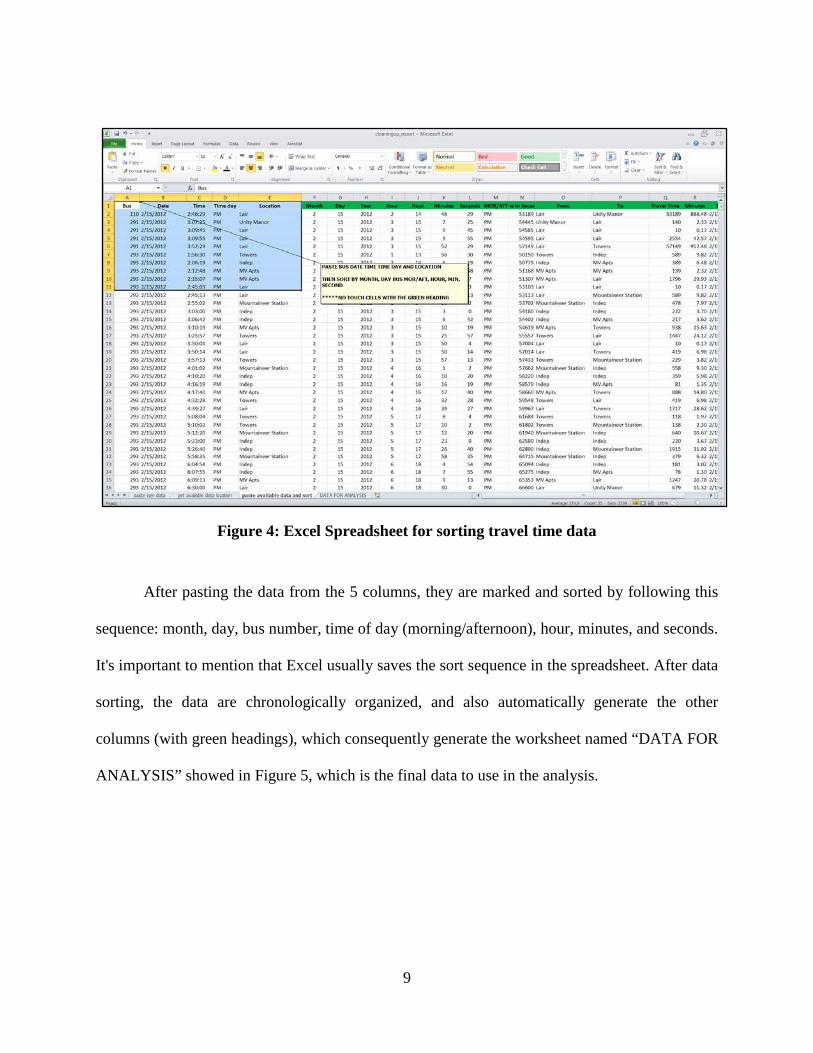
Figure 4: Excel Spreadsheet for sorting travel time data

After pasting the data from the 5 columns, they are marked and sorted by following this

sequence: month, day, bus number, time of day (morning/afternoon), hour, minutes, and seconds.

It's important to mention that Excel usually saves the sort sequence in the spreadsheet. After data

sorting, the data are chronologically organized, and also automatically generate the other

columns (with green headings), which consequently generate the worksheet named “DATA FOR

ANALYSIS” showed in Figure 5, which is the final data to use in the analysis.

9

Figure 5: “DATA FOR ANALYSIS” Spreadsheet

Data stored in “DATA FOR ANALYSIS” are used in another spreadsheet named

“GRAPH AND TABLES” to produce the graphs and tables documented in this report. “DATA

FOR ANALYSIS” columns A through G are copied and pasted into the spreadsheet “GRAPH

AND TABLES” in the worksheet named “ANALYSIS.” This worksheet automatically generates

the worksheet “TABLES_GRAPHS,” which displays the travel time for each road segment

during each day in the year. The worksheets are shown in Figure 6.

10

Figure 6: Excel spreadsheet based procedure for generating graphs and tables

11

Travel time collected by day allows for identifying travel time trends on regular days

versus specific days such as special events, basketball games, football games, etc. The data

include the following information: bus number, date, origin and destination of the road segment,

and travel time for each road segment in minutes (see Table 1).

Table 1: Data Sample

Bus Date From To Travel Time (min)

291 2/15/2012 Unity Manor Lair 2.333

291 2/15/2012 Lair Depot 6.316

293 2/15/2012 Tower MV Apt 16.3

293 2/15/2012 MV Apt Lair 29.933

293 2/15/2012 Lair Mountaineer Station 9.816

293 2/15/2012 Mountaineer Station MV Apt 15.283

293 2/15/2012 MV Apt Tower 15.633

293 2/15/2012 Tower Depot 12.466

293 2/15/2012 Depot Lair 11.65

293 2/15/2012 Lair Tower 6.983

293 2/15/2012 Tower Mountaineer Station 3.816

293 2/15/2012 Mountaineer Station MV Apt 16.633

293 2/15/2012 MV Apt Tower 14.8

2.3.2 Special Events

Special events are defined as particular occurrences affecting the regular travel patterns

of the bus services. Among these events are: sports events (e.g., basketball and football games);

spring break week; summer term. In addition, the travel time during each college semester was

12

considered (e.g., spring, summer and fall semesters). These special events in the year 2012 for

sport events are listed below.

Basketball: Sat., Jan. 7; Sat., Jan. 14; Sat., Jan. 21; Jan. 30; Wed., Feb. 8; Sat., Feb. 11;

Fri., Feb. 24; Tue., Feb. 28;

Football Games: Sat., Sept. 1 (12:00 p.m.); Sat., Sept. 15 (4:30 p.m.); Sat., Sept. 22

(12:00 p.m.); Sat., Sept. 29 (12:00 p.m.); Sat., Oct. 20 (7:00 p.m.); Sat., Nov. 3 (3:00

p.m.); Sat., Nov. 17 (7:00 p.m.); Sat., Dec. 1.

2.3.3 Data Issues

After collectior, handling, and review of the data, missing values and discrepancies were

encountered. These issues are described below.

Data collected during the afternoon contained more missing observations, and more

discrepancies than morning data. A possible cause was forgetting to turn on the sensor

devices in the bus during the afternoon shifts.

Saturdays presented more missing values. This may be because the devices had not been

turned on.

No information was available on Sundays, as the buses don’t operate on Sundays.

Bus number "1100" had the highest number of discrepancies. It may indicate the time

when the buses shift to other buses. In this scenario the last bus is no longer running;

thus, data display large values of travel time, because the route was taken by another bus

number.

Missing values are observed for some days, possibly caused by obstruction to the

satellite, bushes, trees, etc.

13

The analysis was based on the median, because of the large number of missing values and

discrepancies affecting the data. Median is more reliable than the average in these

circumstances.

Special events considered included spring break, basketball games, football games,

commencement, etc.

2.4 Results

Data obtained through email alerts have missing and high values of travel times.

Therefore, larger values (>100 minutes) of travel time for each segment were removed. After

cleaning the data, the median was considered in the analysis. Note that in this work we do not

explicitly model the dwell times, as we do not have the required data (Bertinin and El-Geneidy,

2004; Dueker et al., 2004; El-Geneidy and Vijayakumar, 2011). Figures and tables that

summarized the results for the most relevant period of time over the year are shown in this

section; other figures and tables are documented in the appendix. It is important to highlight that

in situations with a large amount of discrepancies in a data set, the median performed better than

the mean in terms of accuracy. Table 2 shows the median of a regular week collected over the

year (February - November 2012).

14

Table 2: Median Travel Time in a Regular Week

Road Segments Time of Day Monday Tuesday Wednesday Thursday Friday Saturday

Unity Manor - Lair AM 2.33 2.54 2.63 2.87 3.16 1.83

PM 7.39 2.97 2.74 12.19 11.35 1.83

Lair - Towers AM 6.65 6.91 6.57 6.16 7.65 6.98

PM 8.48 6.99 8.57 8.15 7.30 5.45

Towers - Mountaineer Station AM 2.58 2.66 2.84 2.91 2.67 6.73

PM 2.98 3.08 3.18 3.09 3.17 6.98

Mountaineer Station - Indep AM 8.34 8.79 8.35 8.44 8.32 6.98

PM 9.25 8.92 9.44 9.06 9.01 7.21

Indep - MV APT AM 7.94 7.65 7.62 17.16 7.94 PM 4.80 4.54 4.49 4.45 4.97 3.67

Total Travel Time

AM 27.83 28.54 28.02 37.54 29.74 22.53

PM 32.90 26.50 28.41 36.94 35.80 25.13

Figure 7 shows the travel time distributions corresponding to a normal week for the gold line bus

service. The median travel time during weekdays (Monday-Friday) at the morning time was

30.33 minutes and during the afternoon time was 32.11 minutes. Travel time showed variability

over the week; however, during Mondays and Fridays the afternoon travel time was higher than

for morning operations. Saturday seems to be the day with the lowest travel time even though a

value is missing for the afternoon period. It is expected that this is because there are no college

classes during weekends. In addition, the average speed for each road segment was calculated

considering the road segment length and travel time for each segment. The average travel speed

is illustrated in Table 3.

15

Figure 7: Regular Week Travel Time

Table 3: Average Travel Speed



PM 2.14 7.28 3.65 1.77 1.62 11.84

Lair - Towers AM 13.11 12.94 13.61 14.52 11.69 12.80

PM 10.54 12.79 10.09 10.97 12.25 16.42


PM 13.27 12.86 12.46 12.81 12.48 5.67


PM 12.33 12.78 12.08 12.59 12.66 15.81

Indep - MV APT AM 1.81 1.88 1.89 0.84 1.81 PM 3.00 3.17 3.21 3.23 2.90 3.93

Total Travel Time

AM 9.97 9.78 9.96 7.43 9.38 12.39

PM 7.84 10.53 8.75 7.55 7.38 11.10

0.000

5.000

10.000

15.000

20.000

25.000

30.000

35.000

40.000

Monday Tuesday Wednesday Thursday Friday Saturday

AM

PM

16

Table 3 indicates the average speed for each segment and for the total route for the morning and

afternoon period. The average speed was 9.82 miles/hour for the morning and 8.86 miles/hour

for the afternoon time. The average speed for the total route is 9.34 miles/hour.

Figure 8 shows the travel time during spring break. It indicates that the travel time is

similar to the regular week in the year. A lower travel time was expected during this week;

however, it appears that travel time between Independent Apts and Mountain Valley Apts

increased during this week, affecting the total travel time. Saturday shows the lowest travel time

and lower than a regular week. This week shows patterns contrary to the expected; for this

reason, travel time during the spring semester was contrasted with spring break travel time.

Figure 4 shows these plots splitting the morning and afternoon times of day.

Figure 8: Spring Break Travel Time

Figure 9 indicates that during spring break, travel times fall below the regular spring week. It

indicates that data from the spring break week are reasonable. Figures 10 and 11 illustrate the

0.000

5.000

10.000

15.000

20.000

25.000

30.000

35.000

40.000

45.000

50.000


AM

PM

17

comparison of the travel time for each term season: spring, summer, and fall during morning

and afternoon times.

Figure 9: Spring Break Travel Time

Figure 10: Travel Time Comparison (AM)

0.00

10.00

20.00

30.00

40.00

50.00

60.00

Sunday Monday Tuesday Wednesday Thursday Friday Saturday Sunday

Spring AM

Spring PM

Spring Break AM

Spring Break PM

0.00

10.00

20.00

30.00

40.00

50.00

60.00


Spring AM

Summer AM

Fall AM

18

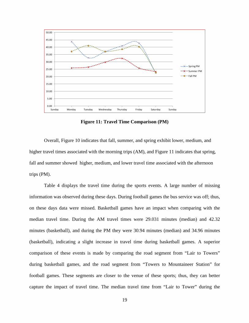
Figure 11: Travel Time Comparison (PM)

Overall, Figure 10 indicates that fall, summer, and spring exhibit lower, medium, and

higher travel times associated with the morning trips (AM), and Figure 11 indicates that spring,

fall and summer showed higher, medium, and lower travel time associated with the afternoon

trips (PM).

Table 4 displays the travel time during the sports events. A large number of missing

information was observed during these days. During football games the bus service was off; thus,

on these days data were missed. Basketball games have an impact when comparing with the

median travel time. During the AM travel times were 29.031 minutes (median) and 42.32

minutes (basketball), and during the PM they were 30.94 minutes (median) and 34.96 minutes

(basketball), indicating a slight increase in travel time during basketball games. A superior

comparison of these events is made by comparing the road segment from “Lair to Towers”

during basketball games, and the road segment from “Towers to Mountaineer Station” for

football games. These segments are closer to the venue of these sports; thus, they can better

capture the impact of travel time. The median travel time from “Lair to Tower” during the

0.00

5.00

10.00

15.00

20.00

25.00

30.00

35.00

40.00

45.00

50.00


Spring PM

Summer PM

Fall PM

19

afternoon was 7.48 min, and during a basketball games was 12.57 min, which indicates that

basketball games’ impact is a 5-minute increase in the travel time. The median travel time from

“Tower to Mountaineer Station” was 3.1 minutes, and during football games was 9 minutes,

indicating a 6-minute increase in travel time.

Table 4: Travel Time for Sport Events

Basketball Football

Road Segments Time of Day 9:00PM 7:00PM 12:00PM 4:30 PM 12:00PM 12:00PM 7:00PM 3:00PM

Unity Manor - Lair AM 25.45 40.42 1.98 2.15 PM 1.73

Lair – Towers AM 7.76 156.30 115.52 7.48 7.65 4.82

PM 12.85 12.29 6.17 338.97 Towers -

Mountaineer Station AM 2.45 3.33 8.15 6.82 7.00

PM 9.35 5.53 8.82 9.07 Mountaineer Station -

Indep AM 8.21 7.04 7.32 9.98 9.15 7.41 6.98

PM 7.98 8.48 6.90 8.56

Indep - MV APT AM 6.20 6.62 PM 4.43 4.23

Total Travel Time AM 42.32 65.16 163.62 127.48 24.78 24.03 18.80

PM 34.60 30.54 23.62 356.59

2.5 Conclusion

This chapter presents a method for collecting, analyzing, and identifying trends in transit

travel times collected during special events versus normal working days. In this case, we focus

on one main route in Morgantown, WV, but the process can be extended to other routes. The

information produced through GPS data has the potential of helping in the planning and

managing of a bus route service. For instance, important information provided is the average

speed of 9.34 miles/hour for the total segment. This indicates that unless changes are made, the

service will not be faster than this speed. Changes in the services or in the roadway network such

20

as a traffic signal or providing fewer bus stop locations along the segment will increase speed

and reduce travel time. The most valuable characteristic of this study is the ability of using data

from GPS devices to obtain important information; this allows transit planners to test various

strategies for improving transit service at low cost, because collection, handling, and analysis of

data are not a complex process, as shown in this study.

21

3.0 Conventional and Flexible Bus Services with Transfer

3.1 Introduction

In urban bus transit networks, it is common to transfer passengers at transfer

terminals because it is prohibitively expensive to provide direct trips for passengers among all

origins and destinations with conventional bus services. Since transfers are important in public

transportation services, it may be beneficial to coordinate bus arrivals at transfer stations

(terminals) so that wait times are minimized and passengers can reliably catch their next bus.

Because bus travel times are usually stochastic in urban transit networks, a probabilistic

optimization model is needed to find buffer times that help provide reliable connections among

buses.

Therefore, this study considered timed transfers coordination. For timed transfers, slack

times improve the reliability of connections and smoothly connect buses at transfer terminals.

Longer slack times increase bus operating cost and users’ waiting cost, but may reduce transfer

cost. Therefore, we needed to develop a probabilistic optimization model for timed transfers

among conventional and flexible bus services. Uncoordinated and coordinated bus operations

were compared through numerical analyses. In order to provide efficient timed transfers, slack

times were optimized numerically. Other decision variables such as headways, fleets, vehicle

sizes were jointly optimized. Thus, optimization models for improving bus transit services are

desirable for better public transportation solutions for users as well as operators.

For a timed transfer analysis, we analyzed a transfer strategy that vehicles do not wait for

other vehicles that arrive behind schedule. We also assumed vehicle arrivals in a timed transfer

station are probabilistically distributed.

22

3.2 Literature Review

3.2.1 Relevant Literature

Kyte et al. (1982) presented a timed-transfer system in Portland, Oregon. They provided

the history of planning, implementation, and evaluation of a timed transfer system that had

provided services since 1979. This system provided timed transfers to the suburban areas in

which demands were low, and provided grid-type bus services to the higher-demand regions.

This paper also discusses the performances and results of the implemented system. They use two

indicators, which are a successful meet and a successful connection, to analyze the transfer

reliabilities. A successful meet is defined as all buses arriving as scheduled at a given time, and a

successful connection is a direct transfer connection that results from two routes arriving as

scheduled. The authors point out that weekday ridership increased by 40 percent after one year of

operation, and local trips using this system increased dramatically. However, the 40% increase in

ridership resulted not only from a timed transfer system, but also from new route designs. Bakker

et al. (1988) similarly studied a multi-centered time transfer system in Austin, Texas, and

confirmed that such a timed transfer system is particularly applicable for low-density cities.

Abkowitz et al. (1987) studied timed transfers between two routes. They compared four

policy cases, namely: unscheduled, scheduled transfer without vehicle waiting, scheduled

transfers where the lower-frequency bus is held until the higher-frequency vehicle arrives, and

scheduled transfers where both buses are held until a transfer event occurs. In other words, this

study compared scheduled, waiting/holding, and double-holding transfer strategies. They noted

that the effectiveness of timed transfers can vary by route conditions. However, they found that

the scheduled transfers are effective (over the unscheduled) when there is incompatibility

between headways and the double-holding strategy outperforms the other time transfer strategies

23

when the headways on intersecting routes are compatible. This study also pointed out that slack

time may be better built into the schedule so that vehicle holding does not cause significant

delays to passengers.

Domschke (1989) explored a schedule coordination problem with the objective of

minimizing waiting times. He provided a mathematical programming formulation which is

generally applicable to a public mass transit network such as subways, trains, and/or buses. The

formulation is a quadratic assignment problem. With four routes and five transfer stations in a

toy network, this study discussed heuristics and a branch and bound algorithm. The heuristics

included a starting heuristic, which was based on rigid regret heuristic, and then a heuristic

improvement procedure. Lastly, simulated annealing (SA) was applied to improve the solutions.

For SA, the quality of the initial solution is important. He found that problems with more than 20

routes could not be solved by exact solution methods.

Knoppers and Muller (1995) provided a theoretical note on transfers in public

transportation. Their main concerns were the transfer time needed and the probability of missed

connection to minimize passengers’ transfer time. They found that when the frequency on the

connecting lines increased, the benefit of transfer coordination yield decreased. Muller and Furth

(2009) tried to reduce passenger waiting time through transfer scheduling and control. They

provided a probabilistic optimization model, and discussed three transfer control types, namely

departure punctuality control, attuned departure control, and delayed departure of connecting

vehicles. They confirmed that by increasing a buffer (slack), the probability of missing the

connection decreases. However, a larger buffer increases the transfer time for people who do not

miss their connection. They also found that if the control policy allowed a bus to be held to make

a connection, the optimal schedule offset decreased.

24

Shrivastava et al. (2002) first discuss existing algorithms for solving nonlinear

mathematical programming, because transit scheduling problems are often nonlinear. The

existing algorithms are generally gradient based, and require at least the first-order derivatives of

both objective and constraint functions with respect to the design variables. With the “slope

tracking” ability, gradient-based methods can easily identify a relative optimum closest to the

initial guess of the optimum design. However, there is no guarantee of locating the global

optimum if the design space is known to be non-convex. In such case, exhaustive and random

search techniques such as random walk or random walk with direction exploitation are quite

useful. The main drawback with these methods is that they often require thousands of function

evaluations, even for the simplest functions, to reach the optimum. They also note that genetic

algorithms (GAs) are based on exhaustive and random search techniques, and are robust for

optimizing nonlinear and non-convex functions. Thus, they apply a GA to schedule coordination

problems. The objective function includes waiting time, transfer time, and in-vehicle time for

users, and vehicle operating cost for operators. For a scheduling problem, they try to solve

routing and scheduling simultaneously. The GA is designed with two substrings, where one

represents routes and the other represents frequencies on those routes. By solving benchmark

problems, they find that genetic algorithms provide better solutions than other heuristics. They

also note that computational times are proportional to the pool size. Cevallos and Zhao (2006)

also use a GA to solve a transfer time optimization problem for a fixed route system. Their main

focus is efficient computational time.

Lee and Schonfeld (1991) studied optimal slack times for coordinating transfers between

rail and bus routes at one terminal. The transfer cost function is formulated as a sum of scheduled

delay cost, missed connection cost for bus to train transfer, and missed connection cost for train

25

to bus transfer. In their paper, the rail transit line was assumed to run on-time (no slack), and

slack times for bus routes were to be optimized. Bus arrivals were assumed to vary

independently from train arrivals so that the joint probabilities of arrivals could be obtained by

simply multiplying the probabilities obtained separately from the bus and train arrivals

distributions. Slack times were optimized analytically, and numerical results show that an

analytic optimization with simplifying assumptions is limited and difficult to solve for complex

situations. Thus, they developed a numerical optimization method to find solutions efficiently.

Ting and Schonfeld (2005) extended Lee and Schofeld (1991)’s study. They explored bus

service coordination in multiple hub networks. They analyzed uncoordinated operations and

coordinated operations, and compared the results. For uncoordinated operation, the formulation

minimizes the total system cost, which is the sum of operating cost, user waiting cost, and user

transfer cost. Transfer cost in uncoordinated operation was simply assumed to be the product of

the average transfer waiting time and the total number of transfer passengers. For the coordinated

operation, the transfer cost consists of slack-time cost, missed connection cost, and dispatching

delay cost. Common headway and integer-ratio headway cases were optimized with a heuristic

algorithm. Their algorithms and numerical results show when coordinated operations with

integer-ratio headways are preferable over uncoordinated operation in terms of total cost.

Simplifying assumptions of this work were that: (1) only one dispatching strategy was

considered, which means vehicles do not wait for other vehicles that arrive behind schedule; (2)

vehicle arrivals on a route were assumed to vary independently from those of other routes, so

that the joint probabilities of arrivals may be obtained by simply multiplying the probabilities

obtained separately from the two vehicle arrival distributions. A limitation of this work is that it

does not ensure integer fleet size.

26

Chen and Schonfeld (2010) adapted the concept of bus transit coordination methods to

freight transportation. They followed the main ideas of joint probabilities and transfer cost

components from some previous transit studies (Lee and Schonfeld, 1991; Ting and Schonfeld,

2005). In this study, they proposed two solution approaches, which are a genetic algorithm and

sequential quadratic programming (SQP) to find good solutions for frequencies and slack times

in intermodal transfers.

Chowdhury and Chien (2002) also studied the coordination of transfers among rail and

feeder bus routes. Their objective was to minimize total cost, including supplier and user costs,

similarly to other studies. They explored various degrees of coordination such as full

coordination, partial coordination, and no coordination. They also followed the assumption of

joint probabilities of independent vehicle arrivals, and assumed that trains operate on-time.

Recently, Chowdhury and Chien (2011) extended a previous study by jointly optimizing bus

size, headway, and slack time for timed transfer. They optimized bus size by assuming maximum

allowable bus headways instead of minimum cost headways. Therefore, their optimized bus size

may be overestimated. For solving this problem they applied Powell’s algorithm (i.e., multi-

variable numerical optimization). Unfortunately, they did not present enough details on the

methodology that might have helped readers understand how joint variables are optimized and

how variables are constrained to be integer. Another limitation of this study is that although it

found optimized vehicle size jointly with other decision variables, such as headways and slack

times, the vehicle size was optimized for only one time period. Optimizing vehicle size and

required fleet size for daily demand or system-wide demand while finding headways and slack

times for each time period represents an opportunity for improvement.

27

3.2.2 Review Summary

No study was found for coordinating transfers among conventional and flexible bus

services, although there are studies on timed transfer coordination for other modes. In evaluating

coordination types, this study explored independent headways and common headways. The

formulations developed here also considered multiple regions. The solution method proposed

here also ensures integer vehicle size(s) as well as integer fleet size(s). Various analyses of

sensitivity to the critical input values should also be conducted.

3.3 Bus Services and Assumptions

3.3.1 System Descriptions

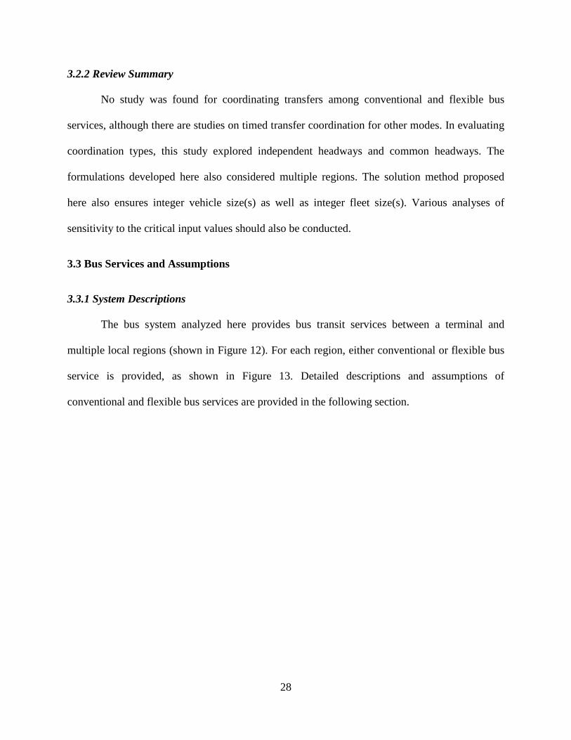
The bus system analyzed here provides bus transit services between a terminal and

multiple local regions (shown in Figure 12). For each region, either conventional or flexible bus

service is provided, as shown in Figure 13. Detailed descriptions and assumptions of

conventional and flexible bus services are provided in the following section.

28

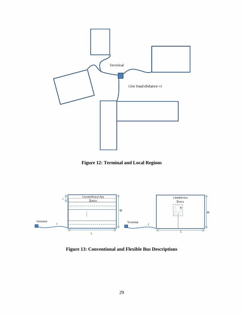
Figure 12: Terminal and Local Regions

Figure 13: Conventional and Flexible Bus Descriptions

29

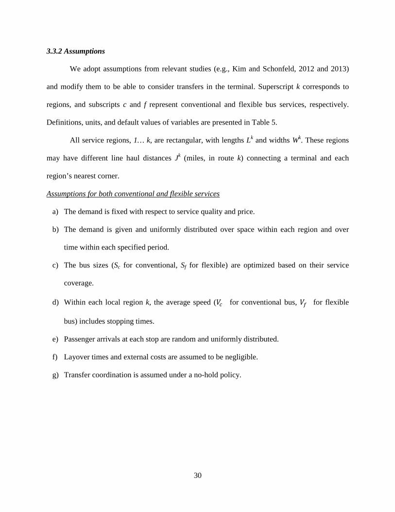
3.3.2 Assumptions

We adopt assumptions from relevant studies (e.g., Kim and Schonfeld, 2012 and 2013)

and modify them to be able to consider transfers in the terminal. Superscript k corresponds to

regions, and subscripts c and f represent conventional and flexible bus services, respectively.

Definitions, units, and default values of variables are presented in Table 5.

All service regions, 1… k, are rectangular, with lengths Lk and widths Wk. These regions

may have different line haul distances Jk (miles, in route k) connecting a terminal and each

region’s nearest corner.

Assumptions for both conventional and flexible services

a) The demand is fixed with respect to service quality and price.

b) The demand is given and uniformly distributed over space within each region and over

time within each specified period.

c) The bus sizes (Sc for conventional, Sf for flexible) are optimized based on their service

coverage.

d) Within each local region k, the average speed (𝑉𝑐 for conventional bus, 𝑉𝑓 for flexible

bus) includes stopping times.

e) Passenger arrivals at each stop are random and uniformly distributed.

f) Layover times and external costs are assumed to be negligible.

g) Transfer coordination is assumed under a no-hold policy.

30

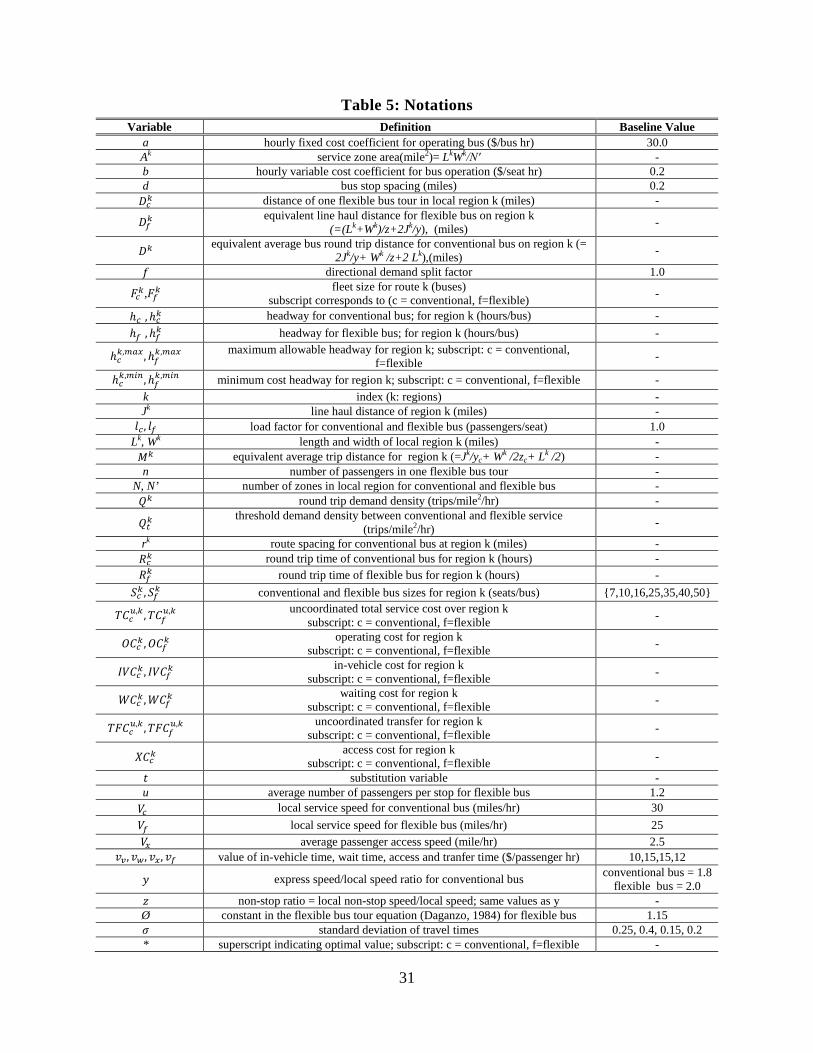
Table 5: Notations Variable Definition Baseline Value

a hourly fixed cost coefficient for operating bus ($/bus hr) 30.0 Ak service zone area(mile2)= LkWk/N′ - b hourly variable cost coefficient for bus operation ($/seat hr) 0.2 d bus stop spacing (miles) 0.2 𝐷𝑐𝑘 distance of one flexible bus tour in local region k (miles) -

𝐷𝑓𝑘 equivalent line haul distance for flexible bus on region k (=(Lk+Wk)/z+2Jk/y), (miles) -

𝐷𝑘 equivalent average bus round trip distance for conventional bus on region k (= 2Jk/y+ Wk /z+2 Lk),(miles) -

𝑓 directional demand split factor 1.0

𝐹𝑐𝑘,𝐹𝑓𝑘 fleet size for route k (buses) subscript corresponds to (c = conventional, f=flexible) -

ℎ𝑐 ,ℎ𝑐𝑘 headway for conventional bus; for region k (hours/bus) - ℎ𝑓 ,ℎ𝑓𝑘 headway for flexible bus; for region k (hours/bus) -

ℎ𝑐 𝑘,𝑚𝑎𝑥,ℎ𝑓

𝑘,𝑚𝑎𝑥 maximum allowable headway for region k; subscript: c = conventional, f=flexible -

ℎ𝑐 𝑘,𝑚𝑖𝑛,ℎ𝑓

𝑘,𝑚𝑖𝑛 minimum cost headway for region k; subscript: c = conventional, f=flexible - k index (k: regions) - Jk line haul distance of region k (miles) - 𝑙𝑐 , 𝑙𝑓 load factor for conventional and flexible bus (passengers/seat) 1.0

Lk, Wk length and width of local region k (miles) - 𝑀𝑘 equivalent average trip distance for region k (=Jk/yc+ Wk /2zc+ Lk /2) - n number of passengers in one flexible bus tour -

N, N’ number of zones in local region for conventional and flexible bus - 𝑄𝑘 round trip demand density (trips/mile2/hr) -

𝑄𝑡𝑘 threshold demand density between conventional and flexible service (trips/mile2/hr) -

rk route spacing for conventional bus at region k (miles) - 𝑅𝑐𝑘 round trip time of conventional bus for region k (hours) - 𝑅𝑓𝑘 round trip time of flexible bus for region k (hours) -

𝑆𝑐𝑘 ,𝑆𝑓𝑘 conventional and flexible bus sizes for region k (seats/bus) {7,10,16,25,35,40,50}

𝑇𝐶𝑐𝑢,𝑘 ,𝑇𝐶𝑓

𝑢,𝑘 uncoordinated total service cost over region k subscript: c = conventional, f=flexible -

𝑂𝐶𝑐𝑘 ,𝑂𝐶𝑓𝑘 operating cost for region k subscript: c = conventional, f=flexible -

𝐼𝑉𝐶𝑐𝑘 , 𝐼𝑉𝐶𝑓𝑘 in-vehicle cost for region k subscript: c = conventional, f=flexible -

𝑊𝐶𝑐𝑘 ,𝑊𝐶𝑓𝑘 waiting cost for region k subscript: c = conventional, f=flexible -

𝑇𝐹𝐶𝑐𝑢,𝑘 ,𝑇𝐹𝐶𝑓

𝑢,𝑘 uncoordinated transfer for region k subscript: c = conventional, f=flexible -

𝑋𝐶𝑐𝑘 access cost for region k subscript: c = conventional, f=flexible -

𝑡 substitution variable - u average number of passengers per stop for flexible bus 1.2 𝑉𝑐 local service speed for conventional bus (miles/hr) 30 𝑉𝑓 local service speed for flexible bus (miles/hr) 25 𝑉𝑥 average passenger access speed (mile/hr) 2.5

𝑣𝑣,𝑣𝑤, 𝑣𝑥, 𝑣𝑓 value of in-vehicle time, wait time, access and tranfer time ($/passenger hr) 10,15,15,12

𝑦 express speed/local speed ratio for conventional bus conventional bus = 1.8 flexible bus = 2.0

𝑧 non-stop ratio = local non-stop speed/local speed; same values as y - Ø constant in the flexible bus tour equation (Daganzo, 1984) for flexible bus 1.15 𝜎 standard deviation of travel times 0.25, 0.4, 0.15, 0.2 * superscript indicating optimal value; subscript: c = conventional, f=flexible -

31

Assumptions for conventional services

a) The region k is divided into Nk parallel zones with a width rk=Wk/Nk for conventional bus,

as shown in Figure 2. Local routes branch from the line haul route segment to run along the

middle of each zone, at a route spacing rk=Wk/Nk.

b) Qk trips/hour, entirely channeled to (or through) the single terminal, are uniformly

distributed over the service area.

c) In each round trip, as shown in Figure 2, buses travel from the terminal a line haul distance

Jk at non-stop speed y𝑉𝑐 to a corner of the local regions, then travel an average of Wk/2

miles at local non-stop speed z𝑉𝑐 from the corner to the assigned zone, then run a local

route of length Lk at local speed 𝑉𝑐 along the central axis of the zone while stopping for

passengers every d miles, and then reverse the above process in returning to the terminal.

Assumptions for flexible services

a) To simplify the flexible bus formulation, region k is divided into N’k equal zones, each

having an optimizable zone area Ak=LkWk/N’k. The zones should be “fairly compact and

fairly convex” (Stein, 1978).

b) Buses travel from the terminal line haul distance Jk at non-stop speed y𝑉𝑓 and an average

distance (Lk+Wk)/2 miles at local non-stop speed z𝑉𝑓 to the center of each zone. They

collect (or distribute) passengers at their door steps through an efficiently routed tour of n

stops and length 𝐷𝑐𝑘 at local speed 𝑉𝑓 . 𝐷𝑐𝑘 is approximated according to Stein (1978), in

which 𝐷𝑐𝑘 = ∅√𝑛𝐴𝑘 , and ∅ = 1.15 for the rectilinear space assumed here (Daganzo,

1984). The values of n and 𝐷𝑐𝑘 are endogenously determined. To return to their starting

32

point the buses retrace an average of (Lk+Wk)/2 miles at z𝑉𝑓 miles per hour and J k miles at

y𝑉𝑓 miles per hour.

c) Buses operate on preset schedules with flexible routing designed to minimize each tour

distance 𝐷𝑐𝑘𝑖 .

d) Tour departure headways are equal for all zones in the region and uniform within each

period.

3.4 Uncoordinated Bus Operations

In this section, we explore uncoordinated bus operations. Conventional and flexible bus

cost functions are formulated, with consideration of transfer cost functions. For both

conventional and flexible bus services, total cost functions consist of bus operating cost, user in-

vehicle cost, user waiting cost, user transfer cost. For conventional bus service, access cost term

is additionally considered.

In the following subsections, we construct cost functions of conventional and flexible bus

services, and analyze them to find optimal values of decision variables such as vehicle sizes, the

number of zones in each region, headways, fleet sizes. In uncoordinated bus operations, we

optimize them analytically.

3.4.1 Conventional Bus Formulation and Analytic Optimization

In the conventional bus cost formulation, we consider bus operating cost, user in-vehicle

cost, user waiting cost, user access cost, and user transfer cost.

𝑇𝐶𝑐𝑢 = ∑ �𝑂𝐶𝑐𝑢,𝑘 + 𝐼𝑉𝐶𝑐

𝑢,𝑘 + 𝑊𝐶𝑐𝑢,𝑘 + 𝑋𝐶𝑐

𝑢,𝑘 + 𝑇𝐹𝐶𝑐𝑢,𝑘�𝐾

𝑘=1 (1)

Conventional bus operating cost, 𝑂𝐶𝑐𝑢,𝑘, can be formulated by multiplying unit bus

operating cost, B, and the number of zones in region k, 𝑁𝑐 𝑢,𝑘, and fleet size, 𝐹𝑐

𝑢,𝑘.

33

𝑂𝐶𝑐𝑢,𝑘 = 𝐵𝑘 ∙ 𝑁𝑐

𝑢,𝑘 ∙ 𝐹𝑐 𝑢,𝑘 (2)

Fleet size, 𝐹𝑐 𝑢,𝑘, can be formulated by

𝐹𝑐 𝑢,𝑘 = 𝐷𝑘

𝑉𝑐∙ℎ𝑐𝑘 (3)

Conventional bus user in-vehicle cost is then formulated by

𝐼𝑉𝐶𝑐𝑢,𝑘 = 𝑣𝑣𝑄𝑘 𝑀

𝑘

𝑉𝑐 (4)

Since we assume that passengers arrive at the stop randomly and uniformly over time, the

waiting time may be estimated as in Welding (1957), Osuna and Newell (1972), and Ting and

Schonfeld (2005).

𝑤𝑘 = 𝐸(ℎ𝑘)2

�1 + (𝜎𝑘)2

�𝐸(ℎ𝑘)�2� (5)

Thus, the waiting cost of uncoordinated conventional bus service is

𝑊𝐶𝑐𝑢,𝑘 = 𝑣𝑤𝑄𝑘𝑤𝑘 = 𝑣𝑤𝑄𝑘 𝐸(ℎ𝑐𝑘)

2�1 + (𝜎𝑘)2

�𝐸(ℎ𝑐𝑘)�2� (6)

As mentioned in Kim and Schonfeld (2012), because the spacing between adjacent

branches of local bus service is 𝑟𝑘, and because service trip origins (or destinations) are

uniformly distributed over the area, the average access distance to the nearest route is one-fourth

of route spacings, 𝑟𝑘/4. Similarly, the access distance alongside the route to the nearest transit

stop is one-fourth of the bus stop spacing, d/4. Therefore, the access cost for the conventional

bus system, 𝑋𝐶𝑐𝑢,𝑘, is

𝑋𝐶𝑐𝑢,𝑘 = 𝑣𝑥∙𝑄𝑘(𝑟𝑘+𝑑)

4𝑉𝑥=

𝑣𝑥∙𝑄𝑘( 𝑊𝑘

𝑁𝑐 𝑢,𝑘+𝑑)

4𝑉𝑥 (7)

Transfer cost, 𝑇𝐹𝐶𝑐𝑢,𝑘, can be similarly formulated to waiting cost function. The only

difference is that the transfer cost considers only transfer demand.

34

𝑇𝐹𝐶𝑐𝑢,𝑘 = 𝑣𝑓𝑄𝑡𝑘𝑤𝑘 = 𝑣𝑓𝑄𝑡𝑘 �

𝐸(ℎ𝑐𝑘)2

+ (𝜎𝑘)2

2𝐸(ℎ𝑐𝑘)� (8)

For the sake of simplicity, the expected value of headway, 𝐸(ℎ𝑘), and the headway, ℎ𝑘,

are interchangeable here. The total cost function of conventional bus service is then

𝑇𝐶𝑐𝑢,𝑘 = 𝐵𝑘 ∙ 𝑁𝑐

𝑢,𝑘 ∙ 𝐹𝑐 𝑢,𝑘 + 𝑣𝑣𝑄𝑘

𝑀𝑘

𝑉𝑐+ 𝑣𝑤𝑄𝑘

𝐸�ℎ𝑘�2

�1 + �𝜎𝑘�2

�𝐸�ℎ𝑘��2� +

𝑣𝑥∙𝑄𝑘�𝑊𝑘

𝑁𝑐 𝑢,𝑘+𝑑�

4𝑉𝑥+ 𝑣𝑓𝑄𝑡𝑘 �

𝐸(ℎ𝑘)2

+ (𝜎𝑘)2

2𝐸(ℎ𝑘)�

(9)

By rearranging Equation 9, we get:


𝑢,𝑘 ∙ 𝐹𝑐 𝑢,𝑘 + 𝑣𝑣𝑄𝑘

𝑀𝑘

𝑉𝑐+ℎ𝑐𝑘

2�𝑣𝑤𝑄𝑘 + 𝑣𝑓𝑄𝑡𝑘� +

𝜎2

2ℎ𝑐𝑘 �𝑣𝑤𝑄

𝑘 + 𝑣𝑓𝑄𝑡𝑘� +𝑣𝑥 ∙ 𝑄𝑘 �

𝑊𝑘

𝑁𝑐 𝑢,𝑘 + 𝑑�

4𝑉𝑥

(10)

Then, we substitute the headway to the fleet size using Equation 3, which is ℎ𝑐𝑘 = 𝐷𝑘

𝑉𝑐∙𝐹𝑐 𝑢,𝑘


𝑢,𝑘 ∙ 𝐹𝑐 𝑢,𝑘 + 𝑣𝑣𝑄𝑘𝑀𝑘

𝑉𝑐+𝐷𝑘�𝑣𝑤𝑄𝑘+𝑣𝑓𝑄𝑡𝑘�

2𝑉𝑐∙𝐹𝑐 𝑢,𝑘 +𝜎2𝑉𝑐∙𝐹𝑐 𝑢,𝑘

�𝑣𝑤𝑄𝑘+𝑣𝑓𝑄𝑡𝑘�

2𝐷𝑘+ 𝑣𝑥∙𝑄𝑘

4𝑉𝑥� 𝑊𝑘

𝑁𝑐 𝑢,𝑘 + 𝑑�

(11)

Equation 11 is now used for optimizing decision variables, namely the number of

zones, 𝑁𝑐 𝑢,𝑘, and fleet sizes, 𝐹𝑐

𝑢,𝑘 .

By taking the partial derivative of 𝑇𝐶𝑐𝑢,𝑘 with respective to the number of zones, 𝑁𝑐

𝑢,𝑘:

∂𝑇𝐶𝑐𝑢,𝑘

∂𝑁𝑐 𝑢,𝑘 = 𝐵𝑘𝐹𝑐

𝑢,𝑘 − 𝑣𝑥∙𝑄𝑘𝑊𝑘

4𝑉𝑥�𝑁𝑐 𝑢,𝑘�

2 = 0 (12)

To guarantee the global minimum solution, we take the second-order derivative of 𝑇𝐶𝑐𝑢,𝑘

with respective to the number of zones, 𝑁𝑐 𝑢,𝑘. As shown in Equation 13, the value of second-

order derivation is positive, so that the optimal value of the number of zones results in the global

minimum.

35

∂2𝑇𝐶𝑐𝑢,𝑘

∂(𝑁𝑐 𝑢,𝑘)2

= 𝑣𝑥∙𝑄𝑘𝑊𝑘

2𝑉𝑥�𝑁𝑐 𝑢,𝑘�

3 > 0 (13)

Rearranging Equation 12, we get

(𝑁𝑐 𝑢,𝑘)2 = − 𝑣𝑥∙𝑄𝑘𝑊𝑘

4𝐵𝑘𝑉𝑥𝐹𝑐 𝑢,𝑘 (14)

Then, we find the optimal fleet size by an analytic optimization. Similarly to the number

of zones, we take the partial derivation of Equation 11 regarding the fleet size, 𝐹𝑐 𝑢,𝑘, as shown in

Equation 15.

∂𝑇𝐶𝑐𝑢,𝑘

∂𝐹𝑐 𝑢,𝑘 = 𝐵𝑘 ∙ 𝑁𝑐

𝑢,𝑘 − 𝐷𝑘�𝑣𝑤𝑄𝑘+𝑣𝑓𝑄𝑡𝑘�

2𝑉𝑐∙�𝐹𝑐 𝑢,𝑘�

2 + 𝜎2𝑉𝑐∙�𝑣𝑤𝑄𝑘+𝑣𝑓𝑄𝑡𝑘�

2𝐷𝑘= 0 (15)

Second-order derivation of Equation 11 with respect to the fleet size, 𝐹𝑐 𝑢,𝑘, is then

∂2𝑇𝐶𝑐𝑢,𝑘

∂(𝐹𝑐 𝑢,𝑘)2

= 𝐷𝑘�𝑣𝑤𝑄𝑘+𝑣𝑓𝑄𝑡𝑘�

𝑉𝑐∙�𝐹𝑐 𝑢,𝑘�

3 > 0 (16)

We notice that Equations 14 and 16 have positive values in all possible input values; thus,

optimized values of the number of zones, 𝑁𝑐 𝑢,𝑘 and fleet size, 𝐹𝑐

𝑢,𝑘 guarantee globally optimum

of the objective function (i.e., Equation 11).

By rearranging Equation 15,

�𝐹𝑐 𝑢,𝑘�

2= (𝐷𝑘)2�𝑣𝑤𝑄𝑘+𝑣𝑓𝑄𝑡

𝑘�𝑉𝑐�+𝜎2𝑉𝑐∙�𝑣𝑤𝑄𝑘+𝑣𝑓𝑄𝑡

𝑘�� (17)

We now take a square to Equation 14 and arrange them as follows.

�𝐹𝑐 𝑢,𝑘�

2= (𝑣𝑥)2∙(𝑄𝑘)2(𝑊𝑘)2

16(𝐵𝑘)2(𝑉𝑥)2(𝑁𝑐 𝑢,𝑘)4

(18)

Now, set Equations 17 and 18 to be equal, and arrange it as the function of the number of zones,

𝑁𝑐 𝑢,𝑘.

16(𝐵𝑘)2(𝑉𝑥)2(𝑁𝑐 𝑢,𝑘)4 − 2(𝑣𝑥)2𝐷𝑘𝐵𝑘(𝑄𝑘)2(𝑊𝑘)2𝑉𝑐𝑁𝑐

𝑢,𝑘 − 𝜎2(𝑣𝑥)2(𝑄𝑘)2(𝑊𝑘)2(𝑉𝑐)2�𝑣𝑤𝑄𝑘 + 𝑣𝑓𝑄𝑡𝑘� = 0

(19)

36

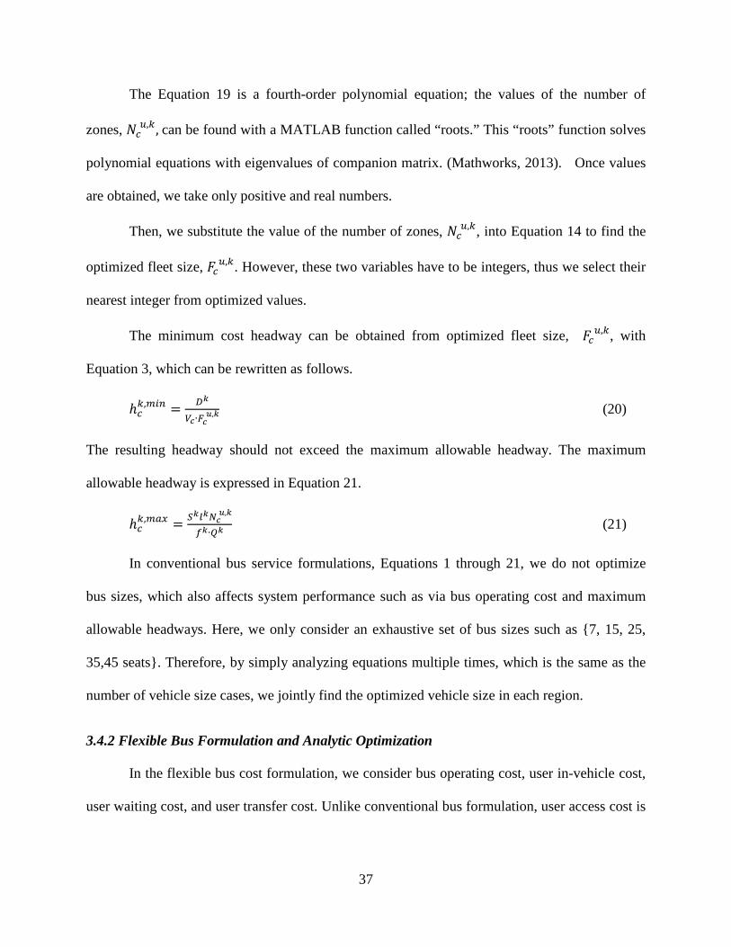
The Equation 19 is a fourth-order polynomial equation; the values of the number of

zones, 𝑁𝑐 𝑢,𝑘, can be found with a MATLAB function called “roots.” This “roots” function solves

polynomial equations with eigenvalues of companion matrix. (Mathworks, 2013). Once values

are obtained, we take only positive and real numbers.

Then, we substitute the value of the number of zones, 𝑁𝑐 𝑢,𝑘, into Equation 14 to find the

optimized fleet size, 𝐹𝑐 𝑢,𝑘. However, these two variables have to be integers, thus we select their

nearest integer from optimized values.

The minimum cost headway can be obtained from optimized fleet size, 𝐹𝑐 𝑢,𝑘, with

Equation 3, which can be rewritten as follows.

ℎ𝑐𝑘,𝑚𝑖𝑛 = 𝐷𝑘

𝑉𝑐∙𝐹𝑐 𝑢,𝑘 (20)

The resulting headway should not exceed the maximum allowable headway. The maximum

allowable headway is expressed in Equation 21.

ℎ𝑐𝑘,𝑚𝑎𝑥 = 𝑆𝑘𝑙𝑘𝑁𝑐

𝑢,𝑘

𝑓𝑘∙𝑄𝑘 (21)

In conventional bus service formulations, Equations 1 through 21, we do not optimize

bus sizes, which also affects system performance such as via bus operating cost and maximum

allowable headways. Here, we only consider an exhaustive set of bus sizes such as {7, 15, 25,

35,45 seats}. Therefore, by simply analyzing equations multiple times, which is the same as the

number of vehicle size cases, we jointly find the optimized vehicle size in each region.

3.4.2 Flexible Bus Formulation and Analytic Optimization

In the flexible bus cost formulation, we consider bus operating cost, user in-vehicle cost,

user waiting cost, and user transfer cost. Unlike conventional bus formulation, user access cost is

37

not included because flexible bus services pick up passengers from their homes to their

destinations, or vice versa.

𝑇𝐶𝑓𝑢 = ∑ �𝑂𝐶𝑓𝑢,𝑘 + 𝐼𝑉𝐶𝑓

𝑢,𝑘 + 𝑊𝐶𝑓𝑢,𝑘 + 𝑇𝐹𝐶𝑓

𝑢,𝑘�𝐾𝑘=1 (22)

Flexible bus operating cost in region k, 𝑂𝐶𝑓𝑢,𝑘, is formulated by multiplying bus operating

cost, 𝐵𝑘, and the number of flexible service zones , 𝑁𝑓 𝑢,𝑘, and the fleet size, 𝐹𝑓

𝑢,𝑘.

𝑂𝐶𝑓𝑢,𝑘 = 𝐵𝑘 ∙ 𝑁𝑓

𝑢,𝑘 ∙ 𝐹𝑓 𝑢,𝑘 (23)

The fleet size, 𝐹𝑓 𝑢,𝑘 is expressed as terms of the equivalent line-haul distance, 𝐷𝑓𝑘, the flexible

bus tour distance in region k, 𝐷𝑐𝑘.

𝐹𝑓 𝑢,𝑘 =

(𝐷𝑓𝑘+𝐷𝑐𝑘)

𝑉𝑓ℎ𝑓𝑘 (24)

The flexible bus tour distance, 𝐷𝑐𝑘, is then formulated by

𝐷𝑐𝑘 = Ø√𝑛𝐴𝑘 (25)

The number of passengers in one tour, n, is shown in Equation 26.

𝑛 =𝐴𝑘𝑄𝑘ℎ𝑓

𝑘

𝑢𝐿𝑘𝑊𝑘 (26)

By substituting Equation 26 and 𝐴𝑘 = 𝐿𝑘𝑊𝑘 𝑁𝑓 𝑢,𝑘� into Equation 25,

𝐷𝑐𝑘 = Ø𝑁𝑓

𝑢,𝑘�𝐿𝑘𝑊𝑘𝑄𝑘ℎ𝑓

𝑘

𝑢 (27)

By substituting Equations 24 and 27 into Equation 23, the flexible bus operating cost is

formulated as follows.

𝑂𝐶𝑓𝑢,𝑘 =

𝐷𝑓𝑘𝐵𝑘𝑁𝑓

𝑢,𝑘

𝑉𝑓ℎ𝑓𝑘 + Ø𝐵𝑘

𝑉𝑓�𝐿𝑘𝑊𝑘𝑄𝑘

𝑢ℎ𝑓𝑘 (28)

The flexible bus in-vehicle cost is then formulated by

38

𝐼𝑉𝐶𝑓𝑢,𝑘=

𝑣𝑣𝑄𝑘(𝐷𝑓𝑘+𝐷𝑐𝑘)

2𝑉𝑓=

𝑣𝑣𝑄𝑘𝐷𝑓𝑘

2𝑉𝑓+ Ø𝑣𝑣𝑄𝑘

2𝑉𝑓𝑁𝑓 𝑢,𝑘�𝐿𝑘𝑊𝑘𝑄𝑘ℎ𝑓

𝑘

𝑢 (29)

As mentioned in Equation 5 earlier, there is an assumption that passengers come to the

terminal randomly and uniformly over time. Therefore, the waiting time in Equation 5 is still

applicable to flexible bus services. Thus the waiting cost of flexible bus service is

𝑊𝐶𝑓𝑢,𝑘 = 𝑣𝑤𝑄𝑘𝑤𝑘 = 𝑣𝑤𝑄𝑘 𝐸(ℎ𝑓

𝑘)

2�1 + (𝜎𝑘)2

�𝐸(ℎ𝑓𝑘)�

2� (30)

The flexible bus transfer cost function is also formulated similarly

𝑇𝐹𝐶𝑓𝑢,𝑘 = 𝑣𝑓𝑄𝑡𝑘𝑤𝑘 = 𝑣𝑤𝑄𝑡𝑘

𝐸(ℎ𝑓𝑘)

2�1 + (𝜎𝑘)2

�𝐸(ℎ𝑓𝑘)�

2� (31)

Similar to conventional bus formulations, the expected value of headway, 𝐸(ℎ𝑓𝑘), and the

headway, ℎ𝑓𝑘, are assumed to be interchangeable in this paper.

By substituting Equations 28 through 31 into Equation 22, the total flexible bus cost in

region k becomes

𝑇𝐶𝑓𝑢,𝑘 =


𝑢,𝑘

𝑉𝑓ℎ𝑓𝑘 + Ø𝐵𝑘

𝑉𝑓�𝐿𝑘𝑊𝑘𝑄𝑘

𝑢ℎ𝑓𝑘 +

𝑣𝑣𝑄𝑘𝐷𝑓𝑘

2𝑉𝑓+ Ø𝑣𝑣𝑄𝑘

2𝑉𝑓𝑁𝑓 𝑢,𝑘

�𝐿𝑘𝑊𝑘𝑄𝑘ℎ𝑓𝑘

𝑢+

𝑣𝑤𝑄𝑘ℎ𝑓𝑘

2+ 𝑣𝑤𝑄𝑘(𝜎𝑘)2

2ℎ𝑓𝑘 +

𝑣𝑓𝑄𝑡𝑘ℎ𝑓

𝑘

2+ 𝑣𝑓𝑄𝑡

𝑘(𝜎𝑘)2

2ℎ𝑓𝑘

(32)

Now, Equation 32 is a function of two decision variables, namely the number of

zones, 𝑁𝑓 𝑢,𝑘, and the headway, ℎ𝑓𝑘. We analytically solve this total cost function. By taking the

partial derivation of Equation 32 with respect to the number of zones, 𝑁𝑓 𝑢,𝑘, we get Equation 33.

∂𝑇𝐶𝑓𝑢,𝑘

∂𝑁𝑓 𝑢,𝑘 =

𝐵𝑘𝐷𝑓𝑘

𝑉𝑓ℎ𝑓𝑘 −

Ø𝑣𝑣𝑄𝑘

2𝑉𝑓�𝐿𝑘𝑊𝑘𝑄𝑘ℎ𝑓

𝑘

𝑢1

(𝑁𝑓 𝑢,𝑘)2

= 0 (33)

Second-order derivation in Equation 34 shows that the total cost function is convex.

∂2𝑇𝐶𝑓𝑢,𝑘

∂(𝑁𝑓 𝑢,𝑘)2

= Ø𝑣𝑣𝑄𝑘

2𝑉𝑓�𝐿𝑘𝑊𝑘𝑄𝑘ℎ𝑓

𝑘

𝑢1

(𝑁𝑓 𝑢,𝑘)3

> 0 (34)

39

By re-writing Equation 33, the number of zones, 𝑁𝑓 𝑢,𝑘, then becomes

𝑁𝑓 𝑢,𝑘 = �

(Ø𝑣𝑣)2𝐿𝑘𝑊𝑘(𝑄𝑘ℎ𝑓𝑘)3

4(𝐵𝑘𝐷𝑓𝑘)2𝑢

4 (35)

To find the optimized headway, we take the partial derivative of the total cost function in

Equation 32 with respect to the headway, ℎ𝑓𝑘.

∂𝑇𝐶𝑓𝑢,𝑘

∂ℎ𝑓𝑘 = −


𝑢,𝑘

𝑉𝑓ℎ𝑓𝑘−2 −

Ø𝐵𝑘

2𝑉𝑓�𝐿𝑘𝑊𝑘𝑄𝑘

𝑢ℎ𝑓𝑘−

32 +

Ø𝑣𝑣𝑄𝑘

4𝑉𝑓𝑁𝑓 𝑢,𝑘 �

𝐿𝑘𝑊𝑘𝑄𝑘

𝑢ℎ𝑓𝑘−

12 +

𝑣𝑤𝑄𝑘+𝑣𝑓𝑄𝑡

𝑘

2−�𝜎𝑘�

2�𝑣𝑤𝑄𝑘+𝑣𝑓𝑄𝑡𝑘�

2ℎ𝑓𝑘−2 = 0

(36)

Second-order derivation is shown in Equation 37 as follows.

∂2𝑇𝐶𝑓𝑢,𝑘

∂(ℎ𝑓𝑘)2

= 2𝐷𝑓𝑘𝐵𝑘𝑁𝑓

𝑢,𝑘

𝑉𝑓ℎ𝑓𝑘−3 + 3Ø𝐵𝑘


𝑢ℎ𝑓𝑘

−52 − Ø𝑣𝑣𝑄𝑘



𝑢ℎ𝑓𝑘

−32 + (𝜎𝑘)2�𝑣𝑤𝑄𝑘 + 𝑣𝑓𝑄𝑡𝑘�ℎ𝑓𝑘−3

(37)

To be a globally convex function, Equation 37 has to be positive with whichever values of

headways. By rearranging Equation 37, we get

�2𝐷𝑓

𝑘𝐵𝑘𝑁𝑓 𝑢,𝑘

𝑉𝑓+ (𝜎𝑘)2�𝑣𝑤𝑄𝑘 + 𝑣𝑓𝑄𝑡𝑘��

1

�ℎ𝑓𝑘3

+ �3Ø𝐵𝑘


𝑢� 1ℎ𝑓𝑘 − � Ø𝑣𝑣𝑄𝑘



𝑢� > 0

(38)

Once we get values of headways, Equation 38 has to be checked.

By rewriting Equation 36,

�−𝐷𝑓𝑘𝐵𝑘𝑁𝑓

𝑢,𝑘

𝑉𝑓− �𝜎𝑘�

2�𝑣𝑤𝑄𝑘+𝑣𝑓𝑄𝑡

𝑘�2

� − Ø𝐵𝑘


𝑢 �ℎ𝑓𝑘 + Ø𝑣𝑣𝑄𝑘



𝑢�ℎ𝑓𝑘

3 +

𝑣𝑤𝑄𝑘+𝑣𝑓𝑄𝑡𝑘

2ℎ𝑓𝑘

2 = 0

(39)

40

We can solve Equations 35 and 39 simultaneously to find the optimized number of zones,

𝑁𝑓 𝑢,𝑘, and the headway, ℎ𝑓𝑘. By substituting Equation 35 into Equation 39, we get

�𝑣𝑤𝑄𝑘+𝑣𝑓𝑄𝑡𝑘�

2ℎ𝑓𝑘

84 −

𝐷𝑓𝑘𝐵𝑘

𝑉𝑓�

(Ø𝑣𝑣)2𝐿𝑘𝑊𝑘�𝑄𝑘�3

4�𝐵𝑘𝐷𝑓𝑘�

2𝑢

4ℎ𝑓𝑘

34 + Ø𝑣𝑣𝑄𝑘


�4�𝐵𝑘𝐷𝑓𝑘�

2𝐿𝑘𝑊𝑘

(Ø𝑣𝑣)2𝑄𝑘𝑢

4

ℎ𝑓𝑘34 − Ø𝐵𝑘


𝑢ℎ𝑓𝑘

24 − �𝜎𝑘�

2�𝑣𝑤𝑄𝑘+𝑣𝑓𝑄𝑡

𝑘�

2= 0

(40)

By substituting ℎ𝑓𝑘14 into t, we get the 8th order polynomial equation that is the function of t.

�𝑣𝑤𝑄𝑘+𝑣𝑓𝑄𝑡𝑘�2

𝑡8 − �𝐷𝑓𝑘𝐵𝑘

𝑉𝑓 �(Ø𝑣𝑣)2𝐿𝑘𝑊𝑘(𝑄𝑘)3

4�𝐵𝑘𝐷𝑓𝑘�

2𝑢

4 + Ø𝑣𝑣𝑄𝑘


�4�𝐵𝑘𝐷𝑓𝑘�

2𝐿𝑘𝑊𝑘

(Ø𝑣𝑣)2𝑄𝑘𝑢

4

� 𝑡3 − Ø𝐵𝑘


𝑢𝑡2 − �𝜎𝑘�

2�𝑣𝑤𝑄𝑘+𝑣𝑓𝑄𝑡𝑘�

2= 0

(41)

Equation 41, which is the function of t, is now solvable with the function called “roots”

as we used in the conventional bus formulation. Once we obtain values of t, we select only

positive and real values. Then, optimal headways are obtained (i.e., ℎ𝑓𝑘 = 𝑡4).

In order to find the number of zones , 𝑁𝑓 𝑢,𝑘, we put the optimized headway into Equation

35. The fleet size, 𝐹𝑓 𝑢,𝑘, is also found by using Equation 24. When we obtain the optimized

number of zones, 𝑁𝑓 𝑢,𝑘 , and the fleet size, 𝐹𝑓

𝑢,𝑘, we need to ensure their integer values, which

means that the optimized headways have to be modified.

The resulting minimum cost headway can be found by substituting Equation 27 into

Equation 24, obtaining

𝐹𝑓 𝑢,𝑘 =

𝐷𝑓𝑘

𝑉𝑓ℎ𝑓𝑘 + Ø

𝑉𝑓𝑁𝑓 𝑢,𝑘 �


𝑢ℎ𝑓𝑘 (42)

After we rearrange Equation 42 to the function of the headway by setting t equal to �1ℎ𝑓𝑘 ,

𝐷𝑓𝑘

𝑉𝑓𝑡2 + Ø

𝑉𝑓𝑁𝑓 𝑢,𝑘 �


𝑢𝑡 − 𝐹𝑓

𝑢,𝑘 = 0 (43)

41

Thus, t can have two values to satisfy Equation 43, however, we take the higher value of t, which

is shown in Equation 44, because the value of t must be positive.

𝑡 = �− Ø𝑉𝑓𝑁𝑓

𝑢,𝑘 �𝐿𝑘𝑊𝑘𝑄𝑘

𝑢+ �( Ø

𝑉𝑓𝑁𝑓 𝑢,𝑘)2�𝐿𝑘𝑊𝑘𝑄𝑘

𝑢+ 4𝐹𝑓

𝑢,𝑘 𝐷𝑓𝑘

𝑉𝑓�

2𝐷𝑓𝑘

𝑉𝑓� (44)

The minimum cost headway that ensures an integer number of zones, 𝑁𝑓 𝑢,𝑘 , and the fleet size,

𝐹𝑓 𝑢,𝑘, is now found in Equation 45.

ℎ𝑓𝑘,𝑚𝑖𝑛 = 4�𝐷𝑓

𝑘�2

�𝑉𝑓�2

⎩⎨

⎧− Ø𝑉𝑓𝑁𝑓

𝑢,𝑘�𝐿

𝑘𝑊𝑘𝑄𝑘𝑢 +�( Ø

𝑉𝑓𝑁𝑓 𝑢,𝑘)

2�𝐿

𝑘𝑊𝑘𝑄𝑘𝑢 +4𝐹𝑓

𝑢,𝑘𝐷𝑓𝑘

𝑉𝑓⎭⎬

⎫2 (45)

As mentioned in conventional bus service formulations, we only consider an exhaustive

set of bus sizes such as {7, 15, 25, 35, 45 seats}. Therefore, by simply analyzing equations

multiple times, which is the same as the number of vehicle size cases, we jointly find the

optimized vehicle size in each region.

3.5 Numerical Evaluations

3.5.1 Base Case Study

Input values

We consider four different regions that are connected to a terminal. The transfer demand,

non-transfer demand, and total demand by route and the size of each region are provided in

Table 6.

42

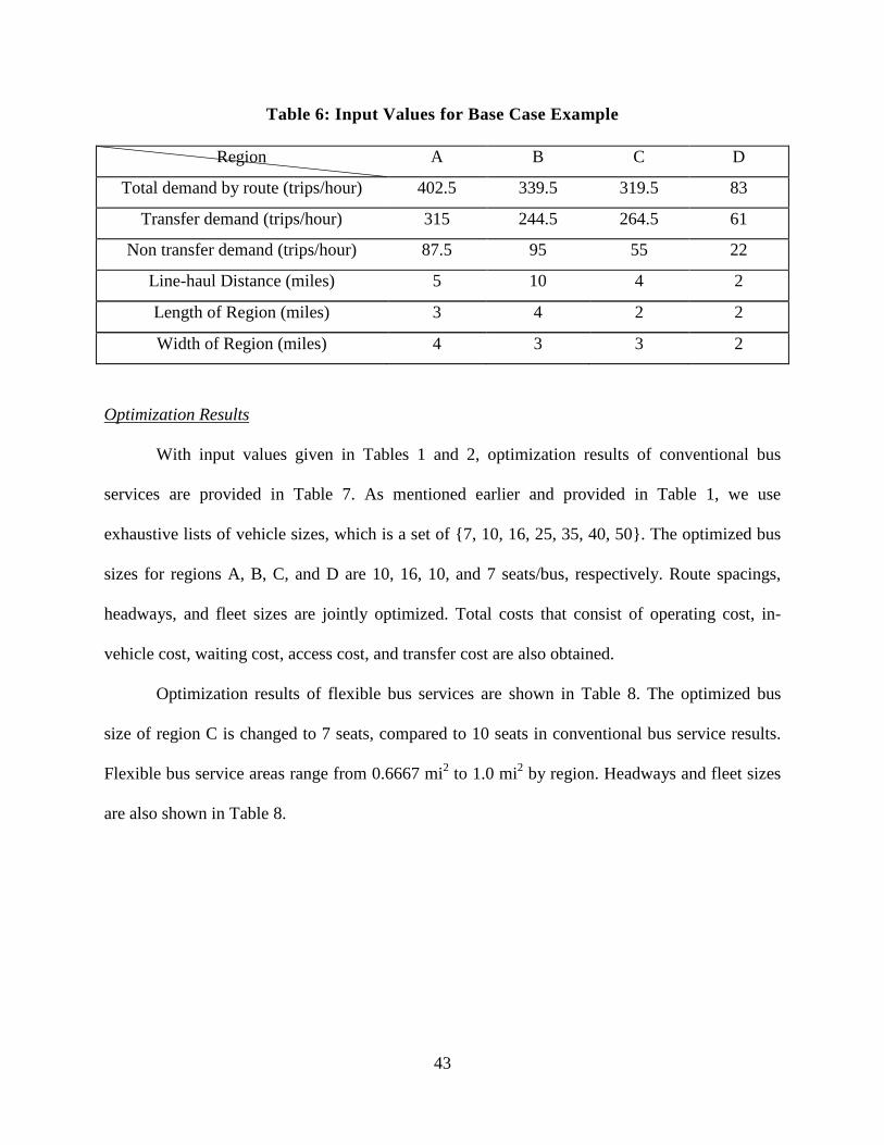
Table 6: Input Values for Base Case Example

Region A B C D

Total demand by route (trips/hour) 402.5 339.5 319.5 83

Transfer demand (trips/hour) 315 244.5 264.5 61

Non transfer demand (trips/hour) 87.5 95 55 22

Line-haul Distance (miles) 5 10 4 2

Length of Region (miles) 3 4 2 2

Width of Region (miles) 4 3 3 2

Optimization Results

With input values given in Tables 1 and 2, optimization results of conventional bus

services are provided in Table 7. As mentioned earlier and provided in Table 1, we use

exhaustive lists of vehicle sizes, which is a set of {7, 10, 16, 25, 35, 40, 50}. The optimized bus

sizes for regions A, B, C, and D are 10, 16, 10, and 7 seats/bus, respectively. Route spacings,

headways, and fleet sizes are jointly optimized. Total costs that consist of operating cost, in-

vehicle cost, waiting cost, access cost, and transfer cost are also obtained.

Optimization results of flexible bus services are shown in Table 8. The optimized bus

size of region C is changed to 7 seats, compared to 10 seats in conventional bus service results.

Flexible bus service areas range from 0.6667 mi2 to 1.0 mi2 by region. Headways and fleet sizes

are also shown in Table 8.

43

Table 7: Optimization Results of Conventional Service

Region A B C D

Bus Size (# of seats) 10 16 10 7

The number of zones (route spacings) 7(0.5714) 5(0.6) 5(0.6) 3(0.6667)

Headway (hours) 0.2294 0.3463 0.1685 0.2444

Fleet size (buses) 14 10 10 3

Operating Cost ($) 448.00 332.00 320.00 94.20

In-Vehicle Cost ($) 723.00 949.34 431.92 73.78

Waiting Cost ($) 1514.80 2058.20 723.75 254.03

Access Cost ($) 465.75 407.40 383.40 107.90

Transfer Cost ($) 948.42 1185.80 479.33 149.36

Total Cost ($) 4100.00 4932.77 2338.40 679.27

Table 8: Optimization Results of Flexible Bus Service

Region A B C D

Bus Size (# of seats) 10 16 7 7

The number of zones (service areas) 13(0.9231) 12(1.0) 9(0.6667) 4(1.0)

Headway (hours) 0.3001 0.4239 0.1972 0.3373

Fleet size (buses) 26 24 18 4

Operating Cost ($) 800.00 796.80 647.73 147.10

In-Vehicle Cost ($) 1207.99 143797 722.00 163.96

Waiting Cost ($) 1534.64 2040.42 745.93 283.81

Transfer Cost ($) 960.82 1175.57 494.02 166.88

Total Cost ($) 4535.44 5451.76 2609.68 761.74

In the base case study, we notice that conventional bus services are economical over

flexible services in all regions. The total cost differences are shown in Table 5. As shown in

44

Table 9, conventional bus services are cheaper than conventional bus services, with 9.5~10.8 %

cost differences.

Table 9: Total Cost Variation between Conventional and Flexible Bus Services

Region A B C D

Conventional Service Total Cost ($) 4100.00 4932.77 2338.40 679.27

Flexible Service Total Cost 4535.44 5451.76 2609.68 761.74

Difference (%)* 9.6 9.5 10.4 10.8

* Difference (%) is computed by (Flexible – Conventional) / Flexible

3.5.2 Sensitivity Analysis

In this sensitivity analysis, we consider variation of time values, namely in-vehicle time,

waiting time, transfer time. Here, we increase time values by 20%, thus values of in-vehicle time,

waiting time, and transfer time are 12, 18, and 14.4 dollars per hour (see Table 10).

Table 10: Total Cost Variations with respect to Sensitivity Cases

Conventional Services Flexible Services

A B C D A B C D

Base Case ($) 4100.0 4932.8 2338.4 679.3 4535.4 5451.8 2609.7 761.7

v_v = 12 ($), 20% up 4244.6 5122.6 2424.8 694.0 4762.7 5698.1 2754.1 792.8

v_w=18($), 20% up 4403.0 5344.4 2483.1 730.1 4841.5 5859.8 2760.0 811.2

v_f=14.4($), 20% up 4289.7 5169.9 2434.3 709.1 4727.5 5686.9 2710.9 790.7

45

Total cost variations in conventional bus services are shown in Figure 14. By increasing

the in-vehicle time value by 20 percent, total cost variations range from 2.17~3.53 % increases

compared to the base case. When increasing the waiting time value by 20 percent, total costs

increase by 6.19~8.34 % over the base case. Here, we notice that cost variations from waiting

time values are larger than sensitivity cases of in-vehicle time and transfer time values. When we

increase transfer time values by 20 percent, total costs of conventional bus services are increased

around 4.1~4.8 %.

Figure 14: Conventional Service Cost Variations

Figure 15 shows total cost changes on flexible bus services with different sensitivity

inputs. The sensitivity case of in-vehicle time value shows that total costs increase from

4.047~5.53%, which are bigger increases compared to conventional bus services, while cost

increments by waiting time values are smaller than those of conventional bus services. When we

increase the transfer time value from $12 to $14.40 per hour, the total cost of flexible bus

46

services increases by 3.8~4.31 percent, which are similar to the variations observed for

conventional bus services.

Figure 15: Flexible Service Cost Variations

3.6 Conclusion

Bus transit services, which consider transfer costs, are formulated for a terminal connecting

multiple local regions. By considering different types of services, which are conventional and

flexible bus services, demand variations better fit to the type of bus services. Besides the type of

bus services, sizes of conventional and flexible buses, the number of zones, headways, and

resulting fleet sizes for uncoordinated bus operations are jointly optimized analytically.

Probabilistically distributed travel times are considered in the modeling. Numerical examples

and its sensitivity analysis are discussed. As an extension, coordinated operations are also

discussed.

47

4.0: References

Advance Tracking Technologies Inc., 2012, http://www.shadowtrackerlive.com/Home.aspx

Abkowitz, M., Josef, R., Tozzi, J., and Driscoll, M. K. 1987, “Operational Feasibility of Timed Transfer in Transit Systems,” Journal of Transportation Engineering, Vol. 113, No. 2, pp. 168-177.

Bakker, J. J., Calkin, J., and Sylvester, S. 1988, “Multi-Centered Time Transfer System for Capital Metro, Austin, Texas,” Transportation Research Record 1202, pp. 22-28.

Bertini, R., and El-Geneidy, A., 2004, “Modeling Transit Trip Time Using Archived Bus Dispatch System Data,” Journal of Transportation Engineering, Vol. 130, No. 1.

Cevallos, F., and Zhao, F. 2006, “A Genetic Algorithm for Bus Schedule Syncronization,” Applications of Advanced Technology in Transportation, Proceedings of the 9th International Conference, Chicago, Illinois.

Chen, C.-C., and Schonfeld, P. 2010, “Modeling and Performance Assessment of Intermodal Transfers at Cargo Terminals,” Transportation Research Record 2162, pp. 53-62.

Chowdhury, M. S., and Chien, S. I.-J. 2002, “Intermodal Transit System Coordination,” Transportation Planning and Technology, Vol. 25, pp. 257-287.

Chowdhury, M. S., and Chien, S. I-J. 2011, “Joint Optimization of Bus Size, Headway and Slack Time for Efficient Timed Transfer,” Transportation Research Record 2218, pp. 48-58.

Domschke, W. 1989, “Schedule Syncronization for Public Transit Networks,” OR Spectrum, Vol. 11, pp. 17-24.

Dueker, K. J., Kimpel, T. J., Strathman, J. G., and Callas, S., “Determinants of Bus Dwell Time,” Journal of Public Transportation, Volume 7, Issue 1, 2004.

El-Geneify, A. E. M, and Vijayakumar, N., 2011, “The effects of articulated buses on dwell and running times,” Journal of Public Transportation, Volume 14, Issue 3.

Kim, M., and Schonfeld, P. 2013, “Integrating Bus Services with Mixed Fleets,” Transportation Research Part B (under review).

Kim, M., and Schonfeld, P., 2012, “Conventional, Flexible and Variable-type Services,” Journal of Transportation Engineering, Vol. 138, No. 3, pp. 263-273.

Knowppers, P., and Muller, T. 1995, “Optimized Transfer Opportunities in Public Transport,” Transportation Science, Vol. 29, No. 1, pp. 101-105.

Kyte, M., Stanley, K., and Gleason, E. 1982, “Planning, Implementing, and Evaluating a Timed-Transfer System in Portland, Oregon,” Transportation Research Record 877, pp. 23-29.

48

http://www.shadowtrackerlive.com/Home.aspx

Lee, K. K. T., and Schonfeld, P. 1991, “Optimal Slack Time for Timed Transfers at a Transit Terminal,” Journal of Advanced Transportation, Vol. 25, No. 3, pp. 282-308.

Lee, K. K., Kuo, S. H. F., and Schonfeld, P. M. 1995, “Optimal Mixed Bus Fleet for Urban Operations,” Transportation Research Record 1503, pp. 39-48.

Mathworks, 2013, “Online Documentation Center,” (http://www.mathworks.com/help/matlab/ref/roots.html?searchHighlight=roots).

Muller, T. H. J., and Furth, P. G. 2009, “Transfer Scheduling and Control to Reduce Passenger Waiting Time,” Transportation Research Record 2112, pp. 111-118.

Shrivastava, P., Dhingra, S. L., and Gundaliya, P. J. 2002, “Application of Genetic Algorithm for Scheduling and Schedule Coordination Problems,” Journal of Advanced Transportation, Vol. 26, No. 1, pp. 23-41.

Ting, C-J., and Schonfeld, P. 2005, “Schedule Coordination in a Multiple Hub Transit Network,” Journal of Urban Planning and Development, Vol. 131, No. 2, pp. 112-124.

49

http://www.mathworks.com/help/matlab/ref/roots.html?searchHighlight=roots

5.0: Appendix

A.1 Travel Time by Route Segment

Figure A.1.1: Unity Manor - Lair

Figure A.1.2: Lair - Towers

0.000

2.000

4.000

6.000

8.000

10.000

12.000

14.000


Unity Manor - Lair (AM)

Unity Manor - Lair (PM)

0.000

1.000

2.000

3.000

4.000

5.000

6.000

7.000

8.000

9.000

10.000


Lair - Towers (AM)

Lair - Towers (PM)

50

Figure A.1.3: Towers - Mountaineer Station

Figure A.1.4: Mountaineer Station - Independence

0.000

1.000

2.000

3.000

4.000

5.000

6.000

7.000

8.000


Towers - Montnair St. (AM)

Towers - Montnair St. (PM)

0.000

1.000

2.000

3.000

4.000

5.000

6.000

7.000

8.000

9.000

10.000


Montainer St. - Indep (AM)

Montainer St. -Indep (PM)

51

Figure A.1.5: Independence - Mountain Valley Apt.

Figure A.1.6: Total Travel Time

0.000

2.000

4.000

6.000

8.000

10.000

12.000

14.000

16.000

18.000

20.000


Indep - MV APT (AM)

Indep - MV APT (PM)

0.000

5.000

10.000

15.000

20.000

25.000

30.000

35.000

40.000


Unity Manor - MV APT (AM)

Unity Manor - MV Apt (PM)

52

A.2. WVU Spring Semester



PM 15.59 6.98 11.52 15.25 15.87 1.82

Lair - Towers AM 5.37 7.03 28.53 8.27 13.83 8.81

PM 12.10 9.96 9.42 9.80 10.41 5.20


PM 3.03 3.11 3.27 2.83 3.30 7.71


PM 8.56 8.51 8.95 8.63 8.73 7.65

Indep - MV APT AM 7.40 6.65 6.58 7.06 7.73 PM 4.45 4.26 3.85 4.45 4.43

Total Travel Time AM 25.29 26.63 48.68 36.60 53.26 23.63

PM 43.73 32.82 37.00 40.95 42.73 22.38

Figure A.2: WVU Spring Semester

0.000

10.000

20.000

30.000

40.000

50.000

60.000


AM

PM

53

A.3 WVU Summer Season



PM 2.50 2.49 2.58 9.78 2.64 2.04

Lair - Towers AM 6.98 6.32 5.98 5.82 6.92 4.00

PM 6.72 6.65 7.50 6.03 5.59 4.50


PM 2.83 3.36 3.13 3.33 2.99 6.40


PM 8.54 8.74 10.07 8.30 8.58 6.78

Indep - MV APT AM 19.32 12.36 20.49 20.21 12.81 PM 5.30 5.25 6.53 4.93 5.97 3.67


PM 25.88 26.48 29.80 32.37 25.77 23.39

Figure A.3: WVU Summer Semester

0.000

5.000

10.000

15.000

20.000

25.000

30.000

35.000

40.000

45.000

50.000


AM

PM

54

A.4 WVU Fall Season



PM 15.75 21.27 23.53 9.44 3.70 2.12

Lair - Towers AM 6.82 6.91 5.32 15.56 7.82 6.23

PM 6.98 6.67 14.80 20.94 5.98


PM 2.98 2.74 2.99 3.11 3.53 7.48


PM 11.39 10.35 10.55 11.36 12.13 7.21

Indep - MV APT AM PM

Total Travel Time

AM 20.47 39.03 19.65 37.57 21.44 22.69

PM 37.11 41.03 37.07 38.70 40.31 22.79

Figure A.4.: WVU Fall Semester

0.000

5.000

10.000

15.000

20.000

25.000

30.000

35.000

40.000

45.000


AM

PM

55

A.5 Spring Break Week



PM 1.92 9.34 11.85 9.03 18.62

Lair - Towers AM 9.71 11.20 5.24 PM 11.56 6.65 5.08 10.48 4.95 4.00


PM 3.26 2.97 3.13 3.30 4.03 9.42


PM 8.17 8.18 7.67 8.75 7.43 6.82

Indep - MV APT AM 18.15 17.65 16.13 17.16 17.71 PM 7.15 5.24 7.38 5.78 7.44


PM 32.06 32.38 35.11 37.34 42.46 20.23

Figure A.5: Travel Time over Spring Break

0.000

5.000

10.000

15.000

20.000

25.000

30.000

35.000

40.000

45.000

50.000


AM

PM

56

A.6. WVU - Final Week


Unity Manor - Lair AM 2.00 2.05 15.96 20.73 36.43 PM 35.83 14.74

Lair - Towers AM 5.37 7.03 13.83 PM 17.08 9.96

Towers - Mountaineer Station AM 24.02 2.79 PM 2.27 2.19 7.17 2.87

Mountaineer Station - Indep AM 8.61 7.62 21.55 8.78 6.98

PM 8.18 8.54 8.51 8.01 9.05 12.32

Indep - MV APT AM 21.06 18.32 6.57 6.07 7.14 PM 5.15 5.15 4.41 4.05


PM 32.67 61.68 20.09 25.61 13.09 12.32

Figure A.6: Final Week Travel Time

0.000

10.000

20.000

30.000

40.000

50.000

60.000

70.000


AM

PM

57

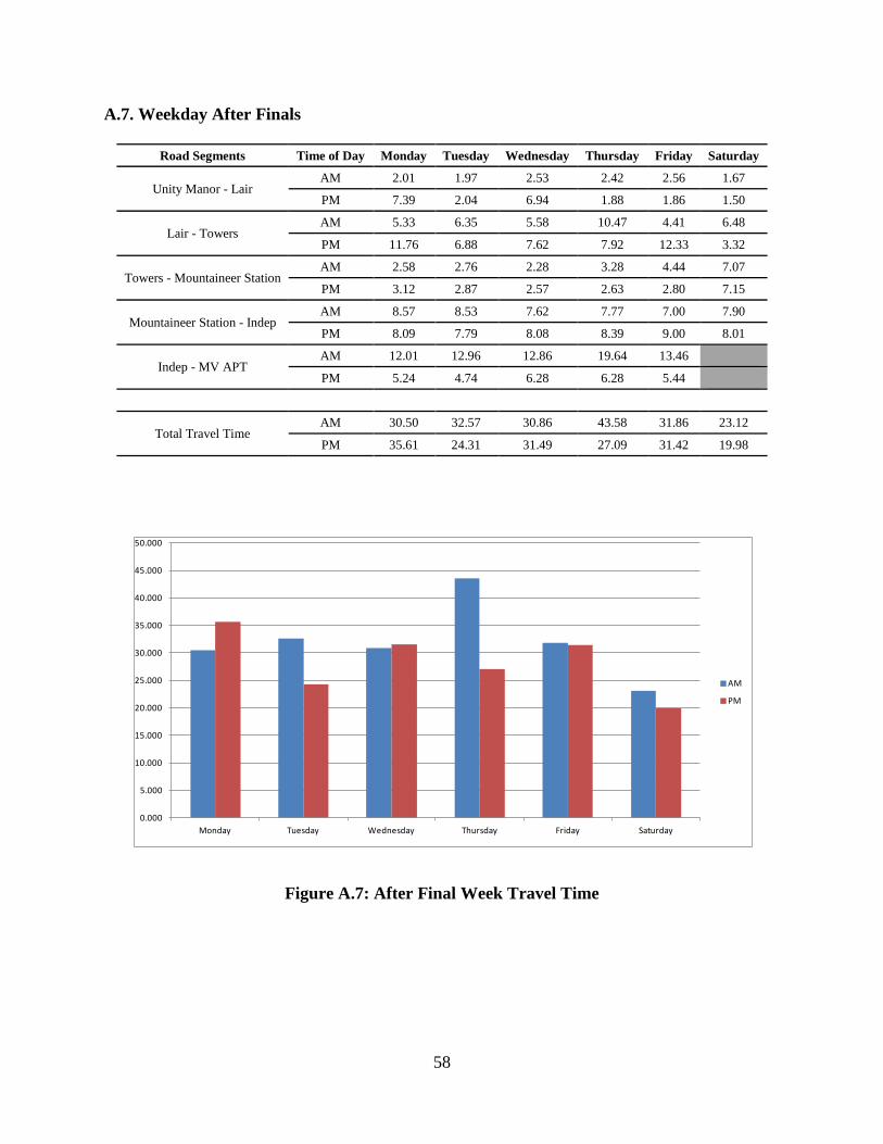
A.7. Weekday After Finals



PM 7.39 2.04 6.94 1.88 1.86 1.50

Lair - Towers AM 5.33 6.35 5.58 10.47 4.41 6.48

PM 11.76 6.88 7.62 7.92 12.33 3.32


PM 3.12 2.87 2.57 2.63 2.80 7.15


PM 8.09 7.79 8.08 8.39 9.00 8.01

Indep - MV APT AM 12.01 12.96 12.86 19.64 13.46 PM 5.24 4.74 6.28 6.28 5.44


PM 35.61 24.31 31.49 27.09 31.42 19.98

Figure A.7: After Final Week Travel Time

0.000

5.000

10.000

15.000

20.000

25.000

30.000

35.000

40.000

45.000

50.000


AM

PM

58

improved methods for operating public … methods for operating public transportation ... improved...

Documents