doi:10.21957/812mkwz370

from Newsletter Number 104 – Summer 2005

Improved prediction of boundary layer clouds

METEOROLOGY

M. Köhler Improved prediction of boundary layer clouds

2 doi:10.21957/812mkwz370

You are having a sunny summer picnic when suddenly low cloud moves in. Instantly, your skin feels a cooling from the drastic change in radiation. Sunlight is reduced by 50 to 70% or 200 to 300Wm-2. Yet infra-red radiative cooling is also reduced by 50 to 100 Wm-2, because the cloud above emits more black body radiation than the colder clear sky. The air temperature sinks by 1°C per hour, the wind picks up and you start to pack up to go home.

It comes as no surprise that low cloud has a commanding impact on climate as well as climate change. If one could magically cover an additional 4% of the globe with low cloud, the global warming resulting from the potential doubling of CO2 could possibly be offset. On the other hand, if the amount of low cloud decreased there could be an unpleasant positive feedback which would accelerate global warming. Unfortunately, current global climate models are split into those that increase low cloud in climate change scenarios and those that produce a decrease.

Turning our attention to weather forecasting, the quality of cloud forecasts still lags significantly that of temperature and circulation above the planetary boundary layer (PBL). Figure 1 compares the skill of ECMWF forecasts relative to persistence for a few typical variables. Cloud appears to be the most difficult to forecast, with the boundary layer variables (i.e. two-metre temperature and ten-metre wind speed) only a little better. Much better predicted are temperature and wind at 850 hPa just above the boundary layer and, quite encouragingly, six-hour accumulated precipitation. Apparently, it is easier to forecast the dynamically forced precipitation than the small residual — the cloud. The errors in cloud forecasts produce errors in the radiation calculations and these in turn affect the PBL temperatures and winds. This skill comparison of a diverse set of variables comes with caveats such as that persistence is a better forecast benchmark for cloud than for precipitation. Yet, this figure illustrates the difficulty of getting good cloud predictions from accurate circulation forecasts.

At ECMWF considerable work has been invested recently in developing an improved representation of low cloud. As a result the simulation of marine stratocumulus improved drastically. Continental stratus also benefited as witnessed specifically in the blocking period of December 2004 over Europe. This article outlines the key aspects of the new planetary boundary layer parametrization scheme which has been incorporated into the ECMWF Integrated Forecast System (IFS) in April 2005. Some of the improvements in cloud cover are highlighted.

This article appeared in the Meteorology section of ECMWF Newsletter No. 104 – Summer 2005, pp. 18–22.

Improved prediction of boundary layer cloudsMartin Köhler

Figure 1 Forecast skill versus persistence against observations of various atmospheric variables over Europe for the year 2004 at 12 UTC. The observations are radiosondes for 500 hPa and 850 hPa variables and SYNOP stations for the rest. Note that SYNOP cloud observations have significant errors and for cloud and precipitation it is questionable how representative local observations are for the model scale. With RMSE as the root mean square error of forecasts or persistence, the skill is defined as

100

80

60

40

20

0

1 2 3Forecast day

4 5

500 hPa geopotential6 h precipitation850 hPa temperature850 hPa vector wind

2 m temperature10 m wind speedTotal cloud cover

Skill

(%)

RMSE (forecast) RMSE (persistence)

1–

M. Köhler Improved prediction of boundary layer clouds

doi:10.21957/812mkwz370 3

New treatment of stratus and stratocumulusWhat are the physical processes needed to adequately model stratus and stratocumulus in particular? And why has it proved so difficult to develop successful parametrizations? Those low clouds are known to cap well-mixed boundary layers. The required vigorous mixing is mainly forced by the strong radiative cooling at the cloud top. This would cool the entire PBL by 10°C per day if not balanced by surface fluxes and entrainment of warm air through the cloud top. Assuming that the stratocumulus topped PBL is a turbulent well-mixed layer there are just three budgets one has to solve: mass, water and heat.

• The mass budget governed by subsidence and cloud-top entrainment predicts the cloud top height.

• The water and heat budgets determine cloud base and cloud water.

The key factors are surface fluxes, cloud top entrainment, solar warming and infra-red cooling.

Writing these three PBL budgets is straightforward, yet many global models strongly underpredict marine stratocumulus clouds. Generally, the problems these models have can be separated in two categories: inadequate representation of physics and inaccurate numerics. Examples of physical problems are a lack of mixing up to cloud top and there being no scientific consensus about cloud top entrainment. Another region of current inconclusive research is the transition from stratocumulus with unbroken cloud decks to trade cumulus with just a few tens of percent of cloud cover. Numerical difficulties arise from the PBL top moving through model levels and the interaction of PBL, convection, cloud and radiation schemes. Maintaining numerical stability whilst using long time-steps is another typical challenge for transport schemes used to simulate low-level cloud.

The main aim in upgrading the PBL parametrization was to improve low-level cloudiness and pave the way towards the unification of the PBL and shallow convection schemes. To achieve that goal the following ingredients were deemed necessary: (a) moist conserved variables, (b) a combined mass-flux/diffusion solver, (c) a treatment of cloud variability, and (d) a treatment of the transition between stratocumulus and shallow convection.

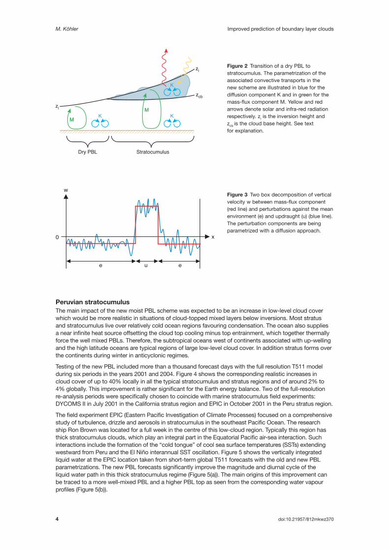
Figure 2 illustrates the approach chosen, which is based on a flux decomposition into diffusion and mass-flux terms. This decomposition goes back to work by Siebesma and Cuijpers at KNMI in 1995, who showed that any vertical flux of a scalar quantity can be split into three contributions: the mass-flux, the sub-core flux and the environmental flux terms. This can be understood by reference to Figure 3. The mass-flux approach (red line) accounts for the strongest updraughts. Then the small perturbations (blue) along the red line can be described with a diffusion approach. This combined mass-flux/diffusion methodology allows for a more accurate description of the fluxes than either approach by itself. Additionally, these two traditional transport approximations can be combined as desired for specific cloud regimes. Therefore, this combined approach is ideally suited to unifying PBL parametrization, which often uses pure diffusion techniques, with convection parametrization, typically based on mass-flux techniques.

Cloud cover and cloud water are treated in the new parametrization scheme by predicting the variance of total water, that is cloud water plus water vapour. If the shape of the probability density function of total water is assumed, the conversion between the prognostic variables water vapour and cloud water on the one hand and total water and total water variance on the other hand can be represented.

The last key requirement of the new PBL parametrization is to determine the PBL cloud regime. In nature there are two typical low-cloud regimes: stratocumulus clouds, which occur in well-mixed PBLs with a large cloud fractions, and trade cumulus clouds with small cloud fractions and cloud layers that are weakly stable stratified. Various algorithms are available to distinguish between these regimes. In the end we used a criterion based on lower tropospheric stability after the work by Klein and Hartmann at the University of Washington in 1993. This criterion reflects the observation that stratocumulus clouds mostly live in atmospheres with strong inversions.

M. Köhler Improved prediction of boundary layer clouds

4 doi:10.21957/812mkwz370

Peruvian stratocumulusThe main impact of the new moist PBL scheme was expected to be an increase in low-level cloud cover which would be more realistic in situations of cloud-topped mixed layers below inversions. Most stratus and stratocumulus live over relatively cold ocean regions favouring condensation. The ocean also supplies a near infinite heat source offsetting the cloud top cooling minus top entrainment, which together thermally force the well mixed PBLs. Therefore, the subtropical oceans west of continents associated with up-welling and the high latitude oceans are typical regions of large low-level cloud cover. In addition stratus forms over the continents during winter in anticyclonic regimes.

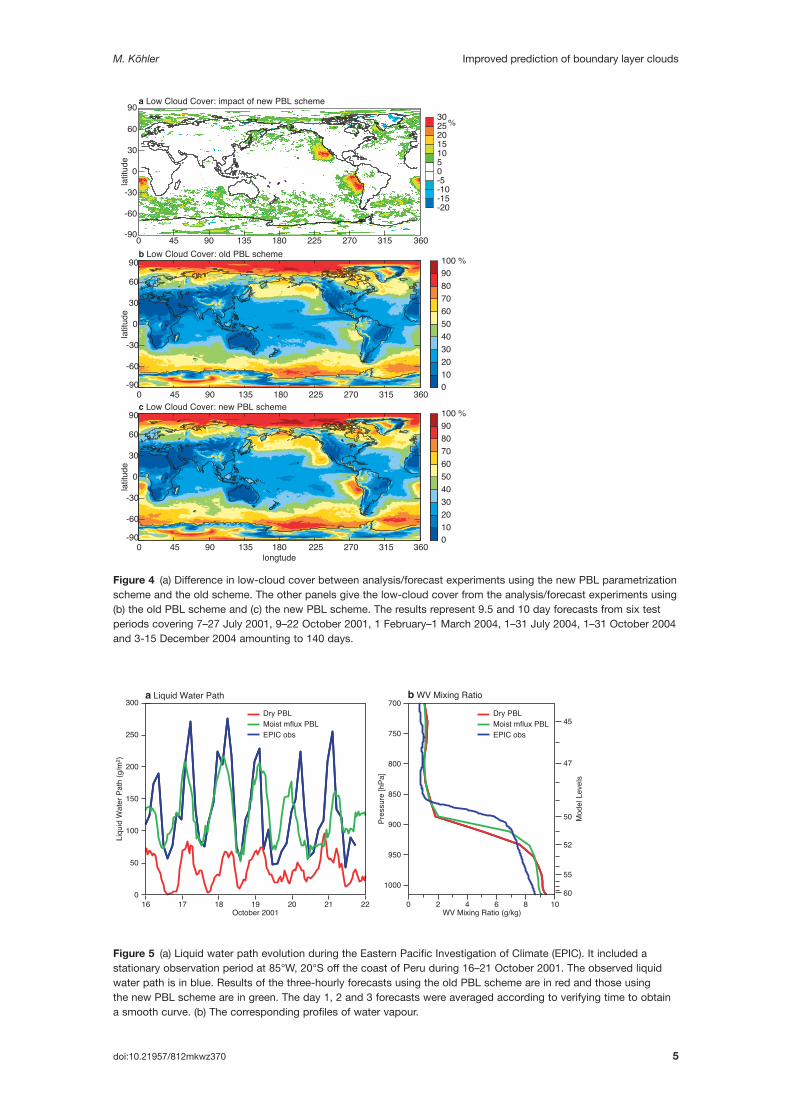
Testing of the new PBL included more than a thousand forecast days with the full resolution T511 model during six periods in the years 2001 and 2004. Figure 4 shows the corresponding realistic increases in cloud cover of up to 40% locally in all the typical stratocumulus and stratus regions and of around 2% to 4% globally. This improvement is rather significant for the Earth energy balance. Two of the full-resolution re-analysis periods were specifically chosen to coincide with marine stratocumulus field experiments: DYCOMS II in July 2001 in the California stratus region and EPIC in October 2001 in the Peru stratus region.

The field experiment EPIC (Eastern Pacific Investigation of Climate Pro cess es) focused on a comprehensive study of turbulence, drizzle and aerosols in stratocumulus in the southeast Pacific Ocean. The research ship Ron Brown was located for a full week in the centre of this low-cloud region. Typically this region has thick stratocumulus clouds, which play an integral part in the Equatorial Pacific air-sea interaction. Such interactions include the formation of the “cold tongue” of cool sea surface temperatures (SSTs) extending westward from Peru and the El Niño interannual SST oscillation. Figure 5 shows the vertically integrated liquid water at the EPIC location taken from short-term global T511 forecasts with the old and new PBL parametrizations. The new PBL forecasts significantly improve the magnitude and diurnal cycle of the liquid water path in this thick stratocumulus regime (Figure 5(a)). The main origins of this improvement can be traced to a more well-mixed PBL and a higher PBL top as seen from the corresponding water vapour profiles (Figure 5(b)).

x

w

0

ue e

Figure 3 Two box decomposition of vertical velocity w between mass-flux component (red line) and perturbations against the mean environment (e) and updraught (u) (blue line). The perturbation components are being parametrized with a diffusion approach.

Dry PBL Stratocumulus

MM

MMK K

K

zi

zi

zcb

Figure 2 Transition of a dry PBL to stratocumulus. The parametrization of the associated convective transports in the new scheme are illustrated in blue for the diffusion component K and in green for the mass-flux component M. Yellow and red arrows denote solar and infra-red radiation respectively. zi is the inversion height and zcb is the cloud base height. See text for explanation.

M. Köhler Improved prediction of boundary layer clouds

doi:10.21957/812mkwz370 5

0 45 90 135 180 225 270 315-90

-60

-30

0

30

60

90

latit

ude

102030405060708090100 %

0

102030405060708090100 %

00 45 90 135 180

longtude225 270 315

-90

-60

-30

0

30

60

90

latit

ude

%

-20-15-10-5051015202530

0 45 90 135 180 225 270 315 360

360

360

-90

-60

-30

0

30

60

90la

titud

e

a Low Cloud Cover: impact of new PBL scheme

b Low Cloud Cover: old PBL scheme

c Low Cloud Cover: new PBL scheme

a�Liquid Water Path

Liqu

id W

ater

Pat

h (g

/m2 )

16 17 18 19 20 21 22October 2001

0

50

100

150

200

250

300Dry PBLMoist mflux PBLEPIC obs

Dry PBLMoist mflux PBLEPIC obs

WV Mixing Ratio (g/kg)

b�WV Mixing Ratio

0 2 4 6 8 10

1000

950

900

850

800

750

700

Pres

sure

[hPa

]

Mod

el L

evel

s

47

52

45

50

55

60

Figure 4 (a) Difference in low-cloud cover between analysis/forecast experiments using the new PBL parametrization scheme and the old scheme. The other panels give the low-cloud cover from the analysis/forecast experiments using (b) the old PBL scheme and (c) the new PBL scheme. The results represent 9.5 and 10 day forecasts from six test periods covering 7–27 July 2001, 9–22 October 2001, 1 February–1 March 2004, 1–31 July 2004, 1–31 October 2004 and 3-15 December 2004 amounting to 140 days.

Figure 5 (a) Liquid water path evolution during the Eastern Pacific Investigation of Climate (EPIC). It included a stationary observation period at 85°W, 20°S off the coast of Peru during 16–21 October 2001. The observed liquid water path is in blue. Results of the three-hourly forecasts using the old PBL scheme are in red and those using the new PBL scheme are in green. The day 1, 2 and 3 forecasts were averaged according to verifying time to obtain a smooth curve. (b) The corresponding profiles of water vapour.

M. Köhler Improved prediction of boundary layer clouds

6 doi:10.21957/812mkwz370

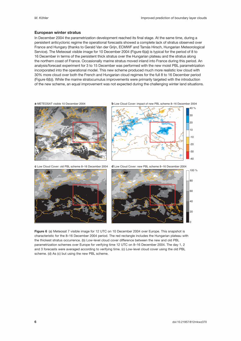
European winter stratusIn December 2004 the parametrization development reached its final stage. At the same time, during a persistent anticyclonic regime the operational forecasts showed a complete lack of stratus observed over France and Hungary (thanks to Gerald Van der Grijn, ECMWF and Tamás Hirsch, Hungarian Meteorological Service). The Meteosat visible image for 10 December 2004 (Figure 6(a)) is typical for the period of 8 to 16 December in terms of the persistent thick stratus over the Hungarian plateau and the stratus along the northern coast of France. Occasionally marine stratus moved inland into France during this period. An analysis/forecast experiment for 3 to 15 December was performed with the new moist PBL parametrization incorporated into the operational model. This new scheme produced much more realistic low cloud with 30% more cloud over both the French and Hungarian cloud regimes for the full 8 to 16 December period (Figure 6(b)). While the marine stratocumulus improvements were primarily targeted with the introduction of the new scheme, an equal improvement was not expected during the challenging winter land situations.

a METEOSAT visible 10 December 2004 b Low Cloud Cover: impact of new PBL scheme 8–16 December 2004

c Low Cloud Cover: old PBL scheme 8–16 December 2004 d Low Cloud Cover: new PBL scheme 8–16 December 2004

-40

-30

-20

-10

10

20

30

40 %

0

20

40

60

80

100 %

Figure 6 (a) Meteosat 7 visible image for 12 UTC on 10 December 2004 over Europe. This snapshot is characteristic for the 8–16 December 2004 period. The red rectangle includes the Hungarian plateau with the thickest stratus occurrence. (b) Low-level cloud cover difference between the new and old PBL parametrization schemes over Europe for verifying time 12 UTC on 8–16 December 2004. The day 1, 2 and 3 forecasts were averaged according to verifying time. (c) Low-level cloud cover using the old PBL scheme. (d) As (c) but using the new PBL scheme.

M. Köhler Improved prediction of boundary layer clouds

doi:10.21957/812mkwz370 7

What did we accomplish and where do we go now?We accomplished the scientifically and technically challenging unification of two conventional approaches for the PBL and convection, the diffusion and mass-flux approaches. That allowed us to unify the two physical boundary layer regimes of the dry and stratocumulus topped PBL with great success.

The same framework is now being extended to include the trade cumulus regime, where this moist combined mass-flux/diffusion approach should be even more appropriate. Early results using a multiple mass-flux extension are very encouraging.

We might never bring the quality of cloud forecasts to the level of 500 hPa height forecasts. But this work shows that there is great potential for improving cloud prediction by careful treatment of their physical and numerical aspects, even though there are physical (e.g. regime transition) and numerical (e.g. inversion prediction) challenges ahead.

Further readingSiebesma, A.P. & J.W.M. Cuijpers, 1995: Evaluation of parametric assumptions for shallow cumulus convection. J. Atmos. Sci., 52, 650–666.

© Copyright 2016

European Centre for Medium-Range Weather Forecasts, Shinfield Park, Reading, RG2 9AX, England

The content of this Newsletter article is available for use under a Creative Commons Attribution-Non-Commercial- No-Derivatives-4.0-Unported Licence. See the terms at https://creativecommons.org/licenses/by-nc-nd/4.0/.

The information within this publication is given in good faith and considered to be true, but ECMWF accepts no liability for error or omission or for loss or damage arising from its use.