improved productivity through the simulation of different
TRANSCRIPT

Improved productivity through the
simulation of different configurations of
resource allocation
by
JM Putter
26127182
Submitted in partial fulfilment of the requirements for the degree
BACHELORS OF INDUSTRIAL ENGINEERING
in the
FACULTY OF ENGINEERING, BUILT ENVIRONMENT, AND INFORMATION TECHNOLOGY
UNIVERSITY OF
PRETORIA
21 October 2009

ii
Abstract
This project document reports on a simulation study of the operations of E-Doc Personnel
in Pretoria. A simulation model is used to evaluate the current process and alternative
scenarios to improve the processing and capturing output of a huge amount of archived
documentation for the South African Police Service onto a database using a custom-
designed information system.
A relevant literature study is documented and the resulting conclusions are discussed. The
document addresses the collection of input data and the concurrent development of a
conceptual model. The translation into the computer model is done by means of the
chosen simulation software, Arena 11.0. The evaluation of alternatives for improvement of
outputs via resource allocation changes are presented and evaluated by making use of the
simulation model.

iii
Contents
Abstract .................................................................................................................................... ii
List of Figures ........................................................................................................................... v
List of Tables ............................................................................................................................ v
1. Introduction ....................................................................................................................... 1
1.1 Background ............................................................................................................... 1
1.2 Process Description .................................................................................................. 1
2. Problem Statement ............................................................................................................ 4
3. Project Aim ......................................................................................................................... 5
4. Project Scope ...................................................................................................................... 6
5. Literature Study .................................................................................................................. 7
5.1 History of Simulation ................................................................................................ 7
5.2 Advantages and uses of Simulation .......................................................................... 8
5.3 Disadvantages of Simulation .................................................................................... 9
5.4 System Concepts ...................................................................................................... 9
5.5 Types of Models ..................................................................................................... 10
5.6 Discrete-Event Simulation ...................................................................................... 10
5.7 Steps in a Simulation Study .................................................................................... 10
5.8 Importance of Input Data ....................................................................................... 12
5.9 Model Verification and Validation .......................................................................... 12
5.10 Time Study .............................................................................................................. 13
6. Conceptual Model and Input Data ................................................................................... 14
6.1 Pages per file .......................................................................................................... 14
6.2 Stage Sections ........................................................................................................ 16
6.3 Stage Processing Times .......................................................................................... 16
6.3.1 Batch-Coding .............................................................................................. 17
6.3.2 Preparation ................................................................................................ 17

iv
6.3.3 Scanning ..................................................................................................... 19
6.3.4 Indexing ...................................................................................................... 21
6.4 Other Factors .......................................................................................................... 22
7. Computer Model .............................................................................................................. 24
7.1 Model verification .................................................................................................. 24
7.2 Model translation ................................................................................................... 24
7.2.1 Stage 1: Batch-coding ................................................................................. 24
7.2.2 Stage 2: Preparation ................................................................................... 25
7.2.3 Stage 3: Scanning ....................................................................................... 25
7.2.2 Stage 4: Indexing ........................................................................................ 26
7.3 Experimental Design ............................................................................................... 31
7.4 Alternatives ............................................................................................................ 32
8. Evaluation ......................................................................................................................... 33
8.1 Utilisation ............................................................................................................... 33
8.2 Daily Output ........................................................................................................... 33
8.3 Queue Lengths ....................................................................................................... 33
8.4 Total Cost ................................................................................................................ 34
9. Conclusion ........................................................................................................................ 35
10. Bibliography .................................................................................................................... 36
Appendix A: Document examples ......................................................................................... 37
Control Form Sheet example .......................................................................................... 37
Time Study example ........................................................................................................ 38
Appendix B: Computer Model .............................................................................................. 39
Appendix C: Arena Reports ................................................................................................... 40
Current Situation ............................................................................................................. 40
Alternative 1 ................................................................................................................... 41
Alternative 2 ................................................................................................................... 42
Alternative 3 ................................................................................................................... 43
Alternative 4 ................................................................................................................... 44

v
List of Figures
Figure 1: Stages of the capturing process .............................................................................. 2
Figure 2: Steps in a simulation study ....................................................................................11
Figure 3: Calculation of standard time ..................................................................................13
Figure 4: Histogram for number of pages per file .................................................................15
Figure 5: Stage 1 – Batch-coding ..........................................................................................28
Figure 6: Stage 2 – Preparation .............................................................................................28
Figure 7: Stage 3 – Scanning .................................................................................................29
Figure 8: Stage 4 – Indexing .................................................................................................30
Figure 9: Resource utilisation of current situation ................................................................31
Figure 10: Current and alternative daily outputs per stage ..................................................34
Figure 11: Computer model ..................................................................................................39
List of Tables
Table 1: Stages, resources and outputs ..................................................................................4
Table 2: Frequency distribution ............................................................................................14
Table 3: Preparation sections ...............................................................................................18
Table 4: Scanning sections ...................................................................................................20
Table 5: Indexing sections ....................................................................................................21
Table 6: Actual and simulated capable output .....................................................................31
Table 7: Current and alternative daily outputs per stage .....................................................33
Table 8: Total cost of alternatives ........................................................................................34

1
1. Introduction
By making use of the knowledge and skills acquired by productivity measurement and
simulating typical real-world situations, the aim of this project is to measure and analyse
the data of a chosen process by making use of time studies. This data will then be used to
construct a simulation model of this process in order to attempt to improve the process
output. For the purpose of this project, a small company called E-Docs Personnel (EDP) was
chosen.
1.1 Background
EDP is a small company that specialises in the execution of temporary paperwork
processes on a contract basis. Currently, they are capturing all the archived and newly
applied public fire-arm licenses and documentation at the SAPS quarters in Silverton
onto a database, making use of an information system designed for this specific
purpose. There are 13 million files that need to be captured and each file size differs
depending on the amount of licenses held by each person and supporting
documentation. The capturing of these files became necessary due to the enormous
amount of space they are occupying.
This capturing process is divided into four stages and will be discussed in more detail
in the process description section of this report. They are:
1. Batch-coding
2. Preparation
3. Scanning
4. Indexing
The product that moves through this process are boxes containing exactly 12 files
each.
1.2 Process Description
A thorough description of each of the four stages (Figure 1) is necessary in order to
clearly understand the entire process of capturing the mentioned files on the
database. As a means of quality control, EDP is making use of a system which requires
for each operator to sign-off on the completion of a file for the specific stage he is
responsible for. This activity is performed onto a control sheet form and an example
of this form is shown in Appendix A.

2
Figure 1: Stages of the capturing process
1. Batch-coding
This is the activity of registering each file onto the information system with the ID
number of the license holder as the unique number. This is the only procedure where
the time taken to perform the activity is entirely independent of the amount of pages
that each file contains. This activity is further broken down into three sub-activities:
• Retrieving a single box from a stack of boxes that were previously retrieved
from the storeroom and removing the files from the box.
• Registering each file onto the system using the unique ID number and producing
a printout of the control sheet that contains the ID number. Signing-off on the
control sheet and inserting it into the file for further use where each operator
has to sign-off on the stage they have performed on a specific file.
• Gathering the files and replacing them into the box. Placing the box onto the
finished stack of boxes waiting to be processed through stage 2.
2. Preparation
This stage consumes most of the time it takes for a box to move through the entire
capturing process. This is where the documentation inside the file is prepared to be
sent through the scanners. This includes the removal of staples, paper clips or any
other fastening devices, the unfolding of the corners of the pages and, if smaller
pieces of paper are present, making a copy of each so that they will fit through the
scanners. This activity is also further broken down into three sub-activities:
• Retrieving a box from the stack of batch-coded boxes.
• Removing a file from the box, preparing each file as discussed above and
signing-off on the control sheet contained in every file.
• Gathering the files and replacing them into the box. Placing the box onto the
finished stack of boxes waiting to be processed through stage 3.
1BATCH-
CODINGPREPARATION
2 3SCANNING
4INDEXING

3
3. Scanning
Scanning is the only stage where mechanical or technical breakdowns can occur and
where maintenance needs to be done on the scanning equipment. This activity consists
of the scanning of both sides of each page of all documents inside the file which is then
stored as images on the database under the specific ID number previously registered
onto the system during the batch-coding stage. The sub-activities are:
• Retrieving a box from the stack of prepared boxes.
• Removing a file from the box and locating the registered ID number on the
system by performing a search for that specific file, inserting and scanning the
pages and signing the control sheet making sure to also indicate the number of
images that were scanned.
• Gathering the files and replacing them into the box. Placing the box onto the
finished stack of boxes waiting to be processed through stage 4.
4. Indexing
In short, during this stage, the scanned pages are put in the right sequence, turned
the right side up and unnecessary pages (blank pages due to the scanning of both
sides of each page) are deleted. The three sub-activities are:
• Retrieving a box from the stack of scanned boxes.
• Removing a file from the box and locating the registered ID number on the
system by performing a search for that specific file. The record and all the
scanned images it contains are then displayed and the indexing activity is
performed as described above.
• Gathering the files and replacing them into the box. Placing the box onto the
finished stack of boxes.

4
2. Problem Statement
At commencement of the contract, a certain amount of boxes as daily output were
established. Currently, the client is not completely satisfied with the actual output rate
achieved every day. As measured by EDP over the past two years, it was found that the
actual average amount of pages per file (34 pages therefore 68 images), was much more
than the original estimated amount (20 pages therefore 40 images), which has a big impact
on the output rate. In order to better understand the problem, reference to three terms
will be used and is defined as follow:
• Target Output – Pre-specified (by client) aim of number of boxes to be processed
per day.
• Current Output – Actual number of boxes processed per day with the process
subjected to bottlenecks and under-utilisation of resources at certain stages.
• Capable Output – Measured, possible output of boxes per day per stage if resource
utilisation is 100% with current configuration.
The current amount of resources available, amount of resources seized per stage, the
current output of boxes (per day) and also the target output, as stipulated by the client, per
stage are as follows:
RESOURCES
(Operators) OUTPUT (Boxes per day)
PROCESS STAGE AVAILABLE SEIZED TARGET CURRENT CAPABLE
Batch-coding (1 printer & 1 pc) 1 1 30 100 105
Preparation 7 1 30 60 60
Scanning (1 scanner) 1 1 30 15 15
Indexing (6 pc’s) 6 1 30 15 95
Table 1: Stages, resources and outputs
Another problem that can be identified from this data is that the output at the Scanning
stage is limiting the output of the Indexing stage (which has a measured capable output of
95 boxes per day), with the effect that the final output is determined by the last stage
(Indexing) and therefore also limited.
The stack of boxes waiting to be prepared and scanned is growing at a high rate every day.
This takes up a lot of space and presents the opportunity to improve the final output if
some resource allocation changes can be made.

5
3. Project Aim
First of all, the standard time for each of the four procedures needs to be determined. The
standard times will then be compared to the daily targets to determine whether the
operators are performing at the desired rate, but more important whether the daily targets
are achievable at the rate the operators have to be able to perform.
The opportunity herein also lies to determine whether or not more boxes can be processed
in one day by making some changes in the resource allocation to the different stages in the
process. The simulation of different scenarios in order to achieve the highest possible
overall resource utilisation will be the main aim of this project.

6
4. Project Scope
For the purpose of this project, the scope of the time studies and simulation will be
focussed on the four stages constituting the document capturing process. The relevant
boundaries, other influencing factors and assumptions made for the purpose of this
simulation, will be further discussed in the conceptual model design section of this report.

7
5. Literature Study
Simulation can be defined as the attempt to imitate a real-life or hypothetical, process or
system over a period of time [11]. By developing a simulation model, the behaviour of the
system can be studied. According to Banks et al. [2], simulation modelling is not only used
as a design tool in order to forecast system performance, but also as an analysis tool in
order to predict the impact of potential changes in a system. According to Oses [8], two
models are necessary when attempting any simulation: First, the conceptual model which
stipulates the set of assumptions made concerning the system operation [2]. Second, the
computer model, which is a translation of the conceptual model into computer code,
making use of the appropriate computer simulation software [3].
5.1 History of Simulation
A brief history of simulation as studied by Kelton et al. [5] is given below.
The Early Years – Late 1950s and 1960s. Large corporations, especially in the steel
and aerospace industry, started using complex simulation models, which at that time
were very expensive tools to use.
The Formative Years – 1970s and early 1980s. The variety of industries making use of
simulation, expanded due to the fact that computers became faster and cheaper.
However, the discovering of simulation by these industries usually only came when
trying to determine why a certain disaster occurred, for instance in the automotive
and heavy industries. Also during this time, simulation became part of operations
research and industrial engineering curricula at many universities.
The Recent Past – Late 1980s. When the personal computer was introduced,
simulation began to play a genuine role in business and became a requirement for
the approval of any major projects.
The Present – 1990s and early 2000s. Smaller firms also began to employ simulation.
Due to improved animation, faster computers and the greater ease of use, simulation
became a standard tool in most businesses and is being employed in even earlier
stages of the design phase. However, the universal acceptance of simulation is still
prevented by the required modelling skills and model-development time.
The Future – With the ever increasing growing rate of computer speed, there is no
doubt that simulation will continue its rapid growth. With the assistance of emerging
and more powerful operating systems, simulation software will become easier to use
with complete integration with other software.

8
5.2 Advantages and uses of Simulation
As stated by Carson [4], simulation can be used for three main reasons:
1. Evaluation
2. Comparison
3. Analysis
Carson [4] also states that the key results of simulation include system performance
prediction and also system problem and cause identification.
The advantages of using simulation have been discussed by many authors, including
among others, Pegden et al. [9] and Banks et al. [2], and a concise summary is as
follows:
• Experimentations including changes, alternatives and options can be
evaluated without disrupting the real system.
• The testing of alternative designs, layouts and transportation systems
becomes possible without committing actual resources.
• A hypothetical system can be modelled to ensure feasibility.
• Better insight into variables, their importance and their interaction can be
acquired.
• In order to better investigate a modelled system, a simulation can be slowed
down or sped up.
• Answering “what if” questions become possible.
• A simulation study can assist in understanding how the real system operates
instead of how it is thought the system operates.
• Analysis can be performed indicating where bottlenecks are forming due to
the forming of queues by materials and work in progress being delayed.
• A simulation can be run numerous times which provides the ability to quickly
gather information repeatedly.
• Visual feedback from the animations helps the user with model development
and validation.
• Simulation is an effective communication tool when trying to prove the
impact a proposed scenario will have.
9
5.3 Disadvantages of Simulation
It is seen that simulation has many advantages, but the above mentioned authors
also discussed some disadvantages and can be summarised as follows:
• Building reliable and accurate simulation models requires a great deal of
time, effort and experience.
• Interpreting simulation results may be difficult due to the fact that
simulation makes use of random inputs, which, in turn produces random
variable outputs.
• Since simulation is so expensive and time consuming, it becomes difficult to
determine the amount of resources to commit to the modelling and analysis
thereof. Holding back on resources may produce an insufficient model.
• The reliance on simulation in order to solve a problem, which, in certain
situations are better to solve using analytical techniques, may produce less
accurate answers to the problem.
5.4 System Concepts
According to Banks [3], there are certain system concepts that require understanding
in order to model and analyse the system. Banks et al. [2] formally define a system as
‘a group of objects that are joined together in some regular interaction or
interdependence toward the accomplishment of some purpose.’ They continue to
define the other important terms which include:
• Entity - ‘An object of interest in the system’
• Attribute - ‘A property of the entity’
• Activity - ‘Time period of specific length’
• State of system - ‘Collection of variables necessary to describe the system
at any time, relative to the objectives of the study’
• Event - ‘Instantaneous occurrence that may change the state of
the system’

10
5.5 Types of Models
Kelton et al. [5] argue that simulation models can be classified in many ways, but that
the three most useful dimensions are:
1. Dynamic vs. Static – Whereas time plays a role in dynamic models, it is
completely irrelevant in the case of static models, also referred to as Monte
Carlo simulation.
2. Discrete vs. Continuous – In discrete models, the state of the system can only
change at discrete points in time when events occur. In continuous models,
continuous change in the system state occurs over time. Mixed continuous-
discrete models are also possible.
3. Stochastic vs. Deterministic – In stochastic models, the input variables are
random, whereas with deterministic models, the inputs are exact known
values. Once again, a model can consist of both random and deterministic
inputs.
5.6 Discrete-Event Simulation
In EDP’s case, the system is time dependant and is therefore dynamic. Also, the
occurrence of change in the system state variables are at discrete points in time.
Banks et al. [2] refer to this type of modelling approach as discrete event simulation.
These types of models are analysed by numerical methods, employing computational
procedures in order to solve the model. However, the model will have both
deterministic and random inputs.
Kelton et al. [5] argue that Arena exhibits the flexibility of simulation languages (such
as SIMAN, GPSS and Simscript), but also the ease of use provided by high-level
simulators.
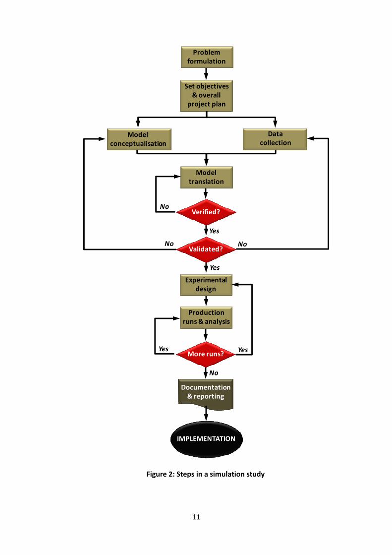
5.7 Steps in a Simulation Study
Carson [4] and Banks et al. [2] provide a comprehensive discussion on the required
steps to assist in building a thorough and accurate model. These steps are illustrated
in Figure 2 on the next page, as extracted from these authors. For the purpose of this
project, these steps will be followed. Other sources such as Law and Kelton [6] and
Pegden et al. [9] provide similar discussions and figures.
11
Figure 2: Steps in a simulation study
Problem
formulation
Set objectives
& overall
project plan
Model
conceptualisation
Data
collection
Model
translation
Verified?
Validated?
Experimental
design
Production
runs & analysis
More runs?
Documentation
& reporting
IMPLEMENTATION
Yes
Yes
Yes Yes
No
No No
No

12
5.8 Importance of Input Data
Banks et al. [2] provide a thorough discussion on the significance of input data for
models. They refer to input data as the ‘driving force for a simulation model’ and
argue that this important step of the simulation study proves to be the biggest task.
Even if a valid model is constructed, inaccurately collected and analysed data will lead
to misleading simulation output. The well known term “GIGO”, or “garbage-in-
garbage-out”, refers to this occurrence.
Banks et al. [2] provide four steps to ensure the development of useful model input
data:
1. Obtain data from the actual system which is to be modelled. Usually, this
takes a considerable amount of time, especially when processing times are
under consideration. Careful and accurate observation is required. In many
cases, data can be extracted from available business records.
2. Determine the most accurate probability distribution to embody the input
data. Available methods include frequency distributions and histograms, but
most modelling software includes tools like these such as Input Analyzer of
Arena.
3. Determine the applicable parameters for the chosen distribution. Input
Analyzer provides for this as well.
4. Assess the chosen distribution and parameters for the accurate
representation of the real data. Formal methods through statistical tests such
as the chi-square test are normally used.
5.9 Model Verification and Validation
These two activities form part of the previously mentioned steps in a simulation study
and play a very important role in order to ensure that the model is an accurate
representation of the actual or hypothetical system which is to be simulated [9].
Balci [1] defines model verification as the activity of confirming that the model
representation is accurately transformed into the computer model, or quoting him,
‘building the model right’.
Sargent [10] defines model validation as confirming that the computerised model
delivers accurate answers, consistent with the simulation model objectives, or
quoting Balci [1], ‘building the right model’.

5.
The data obtained by performing the time studies on the four stages of the process,
will be used as the input data for the simulation model.
random observations of each procedure
As quo
is to add enough time to normal production time to enable the average worker to
meet the standard when performing at standard performance
5.10
The data obtained by performing the time studies on the four stages of the process,
will be used as the input data for the simulation model.
random observations of each procedure
As quo
is to add enough time to normal production time to enable the average worker to
meet the standard when performing at standard performance
10
The data obtained by performing the time studies on the four stages of the process,
will be used as the input data for the simulation model.
random observations of each procedure
•
•
As quo
is to add enough time to normal production time to enable the average worker to
meet the standard when performing at standard performance
Time Study
The data obtained by performing the time studies on the four stages of the process,
will be used as the input data for the simulation model.
random observations of each procedure
• Normal time (obs
NT = Observed time + good pace rating
• Standard time (normal time including allowances for personal needs, basic
fatigue, variable fatigue and unavoidable delays)
ST = NT + Allowance
As quoted from Niebel and Freivalds [7
is to add enough time to normal production time to enable the average worker to
meet the standard when performing at standard performance
Time Study
The data obtained by performing the time studies on the four stages of the process,
will be used as the input data for the simulation model.
random observations of each procedure
Normal time (obs
NT = Observed time + good pace rating
Standard time (normal time including allowances for personal needs, basic
fatigue, variable fatigue and unavoidable delays)
ST = NT + Allowance
ed from Niebel and Freivalds [7
is to add enough time to normal production time to enable the average worker to
meet the standard when performing at standard performance
Fi
Time Study
The data obtained by performing the time studies on the four stages of the process,
will be used as the input data for the simulation model.
random observations of each procedure
Normal time (observed time, but taking into consideration rate of effort)
NT = Observed time + good pace rating
Standard time (normal time including allowances for personal needs, basic
fatigue, variable fatigue and unavoidable delays)
ST = NT + Allowance
ed from Niebel and Freivalds [7
is to add enough time to normal production time to enable the average worker to
meet the standard when performing at standard performance
Figure 3
The data obtained by performing the time studies on the four stages of the process,
will be used as the input data for the simulation model.
random observations of each procedure
erved time, but taking into consideration rate of effort)
NT = Observed time + good pace rating
Standard time (normal time including allowances for personal needs, basic
fatigue, variable fatigue and unavoidable delays)
ST = NT + Allowance
ed from Niebel and Freivalds [7
is to add enough time to normal production time to enable the average worker to
meet the standard when performing at standard performance
gure 3
The data obtained by performing the time studies on the four stages of the process,
will be used as the input data for the simulation model.
random observations of each procedure
erved time, but taking into consideration rate of effort)
NT = Observed time + good pace rating
Standard time (normal time including allowances for personal needs, basic
fatigue, variable fatigue and unavoidable delays)
ed from Niebel and Freivalds [7
is to add enough time to normal production time to enable the average worker to
meet the standard when performing at standard performance
gure 3: Calculati
The data obtained by performing the time studies on the four stages of the process,
will be used as the input data for the simulation model.
random observations of each procedure
erved time, but taking into consideration rate of effort)
NT = Observed time + good pace rating
Standard time (normal time including allowances for personal needs, basic
fatigue, variable fatigue and unavoidable delays)
ed from Niebel and Freivalds [7
is to add enough time to normal production time to enable the average worker to
meet the standard when performing at standard performance
: Calculati
13
The data obtained by performing the time studies on the four stages of the process,
will be used as the input data for the simulation model.
random observations of each procedure and calculating the:
erved time, but taking into consideration rate of effort)
NT = Observed time + good pace rating
Standard time (normal time including allowances for personal needs, basic
fatigue, variable fatigue and unavoidable delays)
ed from Niebel and Freivalds [7], ‘t
is to add enough time to normal production time to enable the average worker to
meet the standard when performing at standard performance
: Calculati
The data obtained by performing the time studies on the four stages of the process,
will be used as the input data for the simulation model.
and calculating the:
erved time, but taking into consideration rate of effort)
NT = Observed time + good pace rating
Standard time (normal time including allowances for personal needs, basic
fatigue, variable fatigue and unavoidable delays)
], ‘the fundamental purpose of all allowances
is to add enough time to normal production time to enable the average worker to
meet the standard when performing at standard performance
: Calculation of standard time
The data obtained by performing the time studies on the four stages of the process,
will be used as the input data for the simulation model.
and calculating the:
erved time, but taking into consideration rate of effort)
NT = Observed time + good pace rating
Standard time (normal time including allowances for personal needs, basic
fatigue, variable fatigue and unavoidable delays)
he fundamental purpose of all allowances
is to add enough time to normal production time to enable the average worker to
meet the standard when performing at standard performance
on of standard time
The data obtained by performing the time studies on the four stages of the process,
will be used as the input data for the simulation model.
and calculating the:
erved time, but taking into consideration rate of effort)
Standard time (normal time including allowances for personal needs, basic
fatigue, variable fatigue and unavoidable delays) –
he fundamental purpose of all allowances
is to add enough time to normal production time to enable the average worker to
meet the standard when performing at standard performance
on of standard time
The data obtained by performing the time studies on the four stages of the process,
will be used as the input data for the simulation model. This is done b
and calculating the:
erved time, but taking into consideration rate of effort)
Standard time (normal time including allowances for personal needs, basic
– ST
he fundamental purpose of all allowances
is to add enough time to normal production time to enable the average worker to
meet the standard when performing at standard performance
on of standard time
The data obtained by performing the time studies on the four stages of the process,
This is done b
erved time, but taking into consideration rate of effort)
Standard time (normal time including allowances for personal needs, basic
ST
he fundamental purpose of all allowances
is to add enough time to normal production time to enable the average worker to
meet the standard when performing at standard performance’, (
on of standard time
The data obtained by performing the time studies on the four stages of the process,
This is done b
erved time, but taking into consideration rate of effort)
Standard time (normal time including allowances for personal needs, basic
he fundamental purpose of all allowances
is to add enough time to normal production time to enable the average worker to
’, (see Figure
The data obtained by performing the time studies on the four stages of the process,
This is done b
erved time, but taking into consideration rate of effort)
Standard time (normal time including allowances for personal needs, basic
he fundamental purpose of all allowances
is to add enough time to normal production time to enable the average worker to
see Figure
The data obtained by performing the time studies on the four stages of the process,
This is done by measuring
erved time, but taking into consideration rate of effort)
Standard time (normal time including allowances for personal needs, basic
he fundamental purpose of all allowances
is to add enough time to normal production time to enable the average worker to
see Figure 3
The data obtained by performing the time studies on the four stages of the process,
y measuring
erved time, but taking into consideration rate of effort)
Standard time (normal time including allowances for personal needs, basic
he fundamental purpose of all allowances
is to add enough time to normal production time to enable the average worker to
3).
The data obtained by performing the time studies on the four stages of the process,
y measuring
erved time, but taking into consideration rate of effort)
Standard time (normal time including allowances for personal needs, basic
he fundamental purpose of all allowances
is to add enough time to normal production time to enable the average worker to
The data obtained by performing the time studies on the four stages of the process,
y measuring
erved time, but taking into consideration rate of effort) - NT
Standard time (normal time including allowances for personal needs, basic
he fundamental purpose of all allowances
is to add enough time to normal production time to enable the average worker to
The data obtained by performing the time studies on the four stages of the process,
y measuring
NT
Standard time (normal time including allowances for personal needs, basic
he fundamental purpose of all allowances
is to add enough time to normal production time to enable the average worker to
The data obtained by performing the time studies on the four stages of the process,
y measuring
Standard time (normal time including allowances for personal needs, basic
he fundamental purpose of all allowances
is to add enough time to normal production time to enable the average worker to

14
6. Conceptual Model and Input Data
The first two steps of the simulation study have already been addressed in the problem
statement and project aim sections of this document. The next step is to develop the
conceptual model and then collect the input data. In reality, these two steps are concurrent
and both will be addressed in this section. This is also where the scope and assumptions
affecting the model will be discussed.
It is critical to collect and use accurate and reliable data as inputs to the model. This is
necessary to ensure that the model produces outputs that resemble that of the real system
as much as possible. This is especially true when working with variable data as in this case.
Therefore, the more data available, the more accurate the probability distributions can be
calculated.
6.1 Pages per file
Fortunately, EDP keeps historical data on all the boxes that have already been
processed. Up to date, the total number of files which have been processed is slightly
more than 570,000. The data relevant to this project concerns the amount of pages
each file contains. This data was extracted from EDP’s information system and a
frequency distribution was calculated using Microsoft Excel, and is shown in Table 2.
Note that the last interval includes 100 to 200 pages. Figure 4 provides a histogram of
this data.
NO. OF PAGES
(BINS) NO. OF FILES
(FREQUENCY)
0 to 10 131
11 to 20 67,946
21 to 30 206,907
31 to 40 160,276
41 to 50 78,629
51 to 60 33,152
61 to 70 13,553
71 to 80 5,396
81 to 90 2,273
91 to 100 964
100 to 200 773
Table 2: Frequency distribution

The next step is to use these 570,000 data points to determine the most suitable
probability distribution to accurately represent them. Arena’s Input Analyzer has the
ability to fit all probability distributions to a given set of data points and then, by
calculating each fitted distri
distribution to represent the set of data points. The extracted text file containing these
data points was imported into the Input Analyzer and the results are as follows:
The next step is to use these 570,000 data points to determine the most suitable
probability distribution to accurately represent them. Arena’s Input Analyzer has the
ability to fit all probability distributions to a given set of data points and then, by
alculating each fitted distri
distribution to represent the set of data points. The extracted text file containing these
data points was imported into the Input Analyzer and the results are as follows:
Fun
-----------------------
Lognormal 0.000346
Gamma 0.000372
Erlang 0.000406
Beta 0.00154
Weibull 0.00316
Normal 0.00866
Exponential 0.0632
Triangular 0.0651
Uniform 0.0918
The next step is to use these 570,000 data points to determine the most suitable
probability distribution to accurately represent them. Arena’s Input Analyzer has the
ability to fit all probability distributions to a given set of data points and then, by
alculating each fitted distri
distribution to represent the set of data points. The extracted text file containing these
data points was imported into the Input Analyzer and the results are as follows:
Function Sq Error
-----------------------
Lognormal 0.000346
Gamma 0.000372
Erlang 0.000406
Beta 0.00154
Weibull 0.00316
Normal 0.00866
Exponential 0.0632
Triangular 0.0651
Uniform 0.0918
Figure 4: Histogram for number of pages per file
The next step is to use these 570,000 data points to determine the most suitable
probability distribution to accurately represent them. Arena’s Input Analyzer has the
ability to fit all probability distributions to a given set of data points and then, by
alculating each fitted distri
distribution to represent the set of data points. The extracted text file containing these
data points was imported into the Input Analyzer and the results are as follows:
ction Sq Error
-----------------------
Lognormal 0.000346
Gamma 0.000372
Erlang 0.000406
Beta 0.00154
Weibull 0.00316
Normal 0.00866
Exponential 0.0632
Triangular 0.0651
Uniform 0.0918
Figure 4: Histogram for number of pages per file
The next step is to use these 570,000 data points to determine the most suitable
probability distribution to accurately represent them. Arena’s Input Analyzer has the
ability to fit all probability distributions to a given set of data points and then, by
alculating each fitted distribution’s square error, determine
distribution to represent the set of data points. The extracted text file containing these
data points was imported into the Input Analyzer and the results are as follows:
ction Sq Error
-----------------------
Lognormal 0.000346
Gamma 0.000372
Erlang 0.000406
Beta 0.00154
Weibull 0.00316
Normal 0.00866
Exponential 0.0632
Triangular 0.0651
Uniform 0.0918
Figure 4: Histogram for number of pages per file
The next step is to use these 570,000 data points to determine the most suitable
probability distribution to accurately represent them. Arena’s Input Analyzer has the
ability to fit all probability distributions to a given set of data points and then, by
bution’s square error, determine
distribution to represent the set of data points. The extracted text file containing these
data points was imported into the Input Analyzer and the results are as follows:
ction Sq Error
-----------------------
Lognormal 0.000346
Gamma 0.000372
Erlang 0.000406
Beta 0.00154
Weibull 0.00316
Normal 0.00866
Exponential 0.0632
Triangular 0.0651
Uniform 0.0918
15
Figure 4: Histogram for number of pages per file
The next step is to use these 570,000 data points to determine the most suitable
probability distribution to accurately represent them. Arena’s Input Analyzer has the
ability to fit all probability distributions to a given set of data points and then, by
bution’s square error, determine
distribution to represent the set of data points. The extracted text file containing these
data points was imported into the Input Analyzer and the results are as follows:
ction Sq Error
-----------------------
Lognormal 0.000346
Gamma 0.000372
Erlang 0.000406
15
Figure 4: Histogram for number of pages per file
The next step is to use these 570,000 data points to determine the most suitable
probability distribution to accurately represent them. Arena’s Input Analyzer has the
ability to fit all probability distributions to a given set of data points and then, by
bution’s square error, determine
distribution to represent the set of data points. The extracted text file containing these
data points was imported into the Input Analyzer and the results are as follows:
ction Sq Error
-----------------------
Figure 4: Histogram for number of pages per file
The next step is to use these 570,000 data points to determine the most suitable
probability distribution to accurately represent them. Arena’s Input Analyzer has the
ability to fit all probability distributions to a given set of data points and then, by
bution’s square error, determine
distribution to represent the set of data points. The extracted text file containing these
data points was imported into the Input Analyzer and the results are as follows:
Figure 4: Histogram for number of pages per file
The next step is to use these 570,000 data points to determine the most suitable
probability distribution to accurately represent them. Arena’s Input Analyzer has the
ability to fit all probability distributions to a given set of data points and then, by
bution’s square error, determine the most suitable
distribution to represent the set of data points. The extracted text file containing these
data points was imported into the Input Analyzer and the results are as follows:
The next step is to use these 570,000 data points to determine the most suitable
probability distribution to accurately represent them. Arena’s Input Analyzer has the
ability to fit all probability distributions to a given set of data points and then, by
the most suitable
distribution to represent the set of data points. The extracted text file containing these

16
The lognormal is therefore the most accurate probability distribution of the set of data
points representing the number of pages each file contains. The lognormal distribution
summary is as follows:
Distribution Summary
Distribution: Lognormal
Expression: 9 + LOGN(25.1, 12.7)
Square Error: 0.000346
Data Summary
Number of Data Points = 570000
Min Data Value = 10
Max Data Value = 179
Sample Mean = 34
Sample Std Dev = 12
6.2 Stage Sections
As mentioned in the process description, each stage is broken up into sections in order
to integrate the facts that:
1. During a stage, either the box as a whole or one of the 12 contained files are
being handled during one of the sections.
2. Processing times vary for each file because of the different amount of
pages/images it contains.
A more thorough breakdown of each stage and the relating processing times will now
be discussed.
6.3 Stage Processing Times
During the different sections of each stage, either of two entities is being processed; a
box containing 12 files, or a file containing a variable amount of pages. A summary of
each stage’s recorded processing times and applicable allowances will now be
discussed. The parameters represent time in seconds.
17
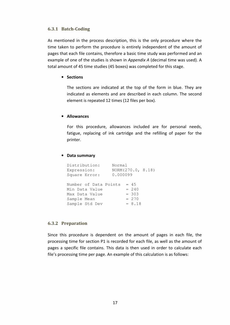
6.3.1 Batch-Coding
As mentioned in the process description, this is the only procedure where the
time taken to perform the procedure is entirely independent of the amount of
pages that each file contains, therefore a basic time study was performed and an
example of one of the studies is shown in Appendix A (decimal time was used). A
total amount of 45 time studies (45 boxes) was completed for this stage.
• Sections
The sections are indicated at the top of the form in blue. They are
indicated as elements and are described in each column. The second
element is repeated 12 times (12 files per box).
• Allowances
For this procedure, allowances included are for personal needs,
fatigue, replacing of ink cartridge and the refilling of paper for the
printer.
• Data summary
Distribution: Normal
Expression: NORM(270.0, 8.18)
Square Error: 0.000099
Number of Data Points = 45
Min Data Value = 240
Max Data Value = 303
Sample Mean = 270
Sample Std Dev = 8.18
6.3.2 Preparation
Since this procedure is dependent on the amount of pages in each file, the
processing time for section P1 is recorded for each file, as well as the amount of
pages a specific file contains. This data is then used in order to calculate each
file’s processing time per page. An example of this calculation is as follows:

18
ELEMENT SECTION TIMES (sec) sec /
page Box no. File Pages P0 P1 P2
8 6
1 42 402 9.57
2 40 380 9.50
3 22 208 9.45
4 29 276 9.52
5 33 323 9.79
6 27 242 8.96
7 35 330 9.43
8 76 736 9.68
9 58 551 9.50
10 20 174 8.70
11 24 240 10.00
12 28 266 9.50
12
TOTAL 6 4128 12
The processing of 20 boxes (240 files) was observed and the times were
recorded. Once again, Input Analyzer will be used to fit all probability
distributions to the data points representing the calculated processing time per
page for all 240 files. Table 3 provides a more detailed description of each
section.
• Sections
SECTION DESCRIPTION
P0 (Set-up) Get box, position box and tools on table & open box.
P1 (Procedure) Remove one file from the box. Preparation includes
paging through & checking of file: remove staples &
binders, unfold corners of papers, tear loose of
double pages, remove & photocopy of smaller
pieces of paper, check page numbers & sort pages
where applicable. Recollect pages, attach photos,
copied pages & smaller pieces of paper to file using a
stapler, close file and sign the control form. Replace
file into box. (x12)
P2 (Finish) Close box & return to finished stack of boxes, clean
work area.
Table 3: Preparation sections

19
• Allowances
For this procedure, allowances included are for personal needs,
fatigue, copying of smaller pieces of paper and other.
• Data summary
P0 (Set-up) : Distribution: Triangular
Expression: TRIA(5.50, 6.10, 6.50)
Square Error: 0.002873
Number of Data Points = 20
Min Data Value = 5.5
Max Data Value = 6.5
Sample Mean = 6.0
Sample Std Dev = 0.2
P1 (Procedure) : Distribution: Normal
Expression: NORM(8.50, 0.40)
Square Error: 0.000281
Number of Data Points = 240
Min Data Value = 7.9
Max Data Value = 10.8
Sample Mean = 8.5
Sample Std Dev = 0.4
P2 (Finish) : Distribution: Triangular
Expression: TRIA(8.80, 11.80, 13.20)
Square Error: 0.002873
Number of Data Points = 20
Min Data Value = 8.8
Max Data Value = 13.2
Sample Mean = 11.3
Sample Std Dev = 0.9
6.3.3 Scanning
This procedure is also dependant on the amount of pages in each file. Another
factor that influences the times is the fact that the scanner sometimes delays the
scanning process if torn or folded pages are sent through. The thickness of
different pages does not have a very big influence on this process and can be
discarded. Again, the processing time for section S1 is recorded for each file, as
well as the amount of pages a specific file contains. This data is then used in
order to calculate each file’s processing time per page. The processing of 30
boxes (360 files) was observed and the times were recorded. Table 4 provides a
more detailed description of each section.

20
• Sections
SECTION DESCRIPTION
S0 (Set-up) Get box, position box on table & open box.
S1 (Procedure) Remove one file from the box. Search for ID number on
system. Open file, remove pages and insert stack of
pages into scanner, control the sending through of
pages by finger, remove stack of scanned pages from
scanner when finished, check on computer amount of
scanned images (double-sided). Replace stack of pages
into file, write down the amount of scanned images
and sign the control form. Close file and stamp with
“SCANNED”-stamp. Replace file into box. (x12)
S2 (Finish) Close box & return to finished stack of boxes.
Table 4: Scanning sections
• Allowances
For this procedure allowances included are for personal needs, fatigue,
reloading of scanner for very large files, removing and reinserting of
stack pages if error occurs.
• Data summary
S0 (Set-up) : Distribution: Triangular
Expression: TRIA(5.60, 6.20, 6.50)
Square Error: 0.037840
Number of Data Points = 30
Min Data Value = 5.6
Max Data Value = 6.5
Sample Mean = 6.1
Sample Std Dev = 0.2
S1 (Procedure) : Distribution: Normal
Expression: NORM(4.50, 0.40)
Square Error: 0.002975
Number of Data Points = 360
Min Data Value = 4.26
Max Data Value = 6.67
Sample Mean = 4.50
Sample Std Dev = 0.4

21
S2 (Finish) : Distribution: Triangular
Expression: TRIA(7.80, 8.20, 8.80)
Square Error: 0.002873
Number of Data Points = 30
Min Data Value = 7.8
Max Data Value = 8.8
Sample Mean = 8.3
Sample Std Dev = 0.2
6.3.4 Indexing
Once again, this procedure is also dependant on the amount of pages in each file
and the observed times and number of pages per file will be used to calculate the
processing time per page.
The processing of 40 boxes (480 files) was observed and the times were
recorded. Table 5 provides a more detailed description of each section.
• Sections
SECTION DESCRIPTION
I0 (Set-up) Get box, position box on table & open box.
I1 (Procedure)
Remove one file from the box and locate the ID number
on system. Delete blank pages using the thumbnail
view (every second page – although care has to be
taken not to delete a page that appears to be blank, but
might have a date stamped or signature on it or on the
back of the page). Using the full screen view, page
through pages and check that pages are present and in
the correct order. Mark the new legislation and archive
sections and perform other required operations on
system. Sign the control form, close file and replace file
into box. (x12)
I2 (Finish) Close box & return to finished stack of boxes.
Table 5: Indexing sections
• Allowances
For this procedure allowances included are for personal needs and
fatigue.

22
• Data summary
I0 (Set-up) : Distribution: Triangular
Expression: TRIA(5.60, 6.20, 6.50)
Square Error: 0.037840
Number of Data Points = 30
Min Data Value = 5.6
Max Data Value = 6.5
Sample Mean = 6.1
Sample Std Dev = 0.2
I1 (Procedure) : Distribution: Normal
Expression: NORM(4.80, 0.32)
Square Error: 0.002279
Number of Data Points = 480
Min Data Value = 4.00
Max Data Value = 5.90
Sample Mean = 4.80
Sample Std Dev = 0.32
I2 (Finish) : Distribution: Triangular
Expression: TRIA(7.80, 8.20, 8.80)
Square Error: 0.002873
Number of Data Points = 30
Min Data Value = 7.8
Max Data Value = 8.8
Sample Mean = 8.3
Sample Std Dev = 0.2
6.4 Other Factors
There are other factors that need to be mentioned in order to model an accurate
representation of the real system:
• Storeroom – The retrieval of boxes from the storeroom, which are to be
processed, and the returning of finished boxes to the storeroom will not be
included in the simulation. The reason for this is because this activity is not
performed by an EDP resource and availability of boxes entering the process
is therefore instantaneous.
• Maintenance – Scanners need to be serviced after 10,000 pages (20,000
images) have been processed. This usually takes about 20 minutes, give or
take a minute.

23
• Breakdowns – This refers to paper jams and laser problems with the
scanners. These occur randomly with an exponential distribution. Paper jams
with a mean of 4 minutes and laser problems with a mean of 45 minutes.
• Lunchtime – Working hours are from 08:00 – 17:00 each day and includes
one hour for lunch. To model this, the simulation will only be run until 16:00,
excluding the lunchtime hour.
• Warm-up period – In the real system, at the start of a working day, there are
boxes ready to be processed at each stage. Therefore, a warm-up period is
required in order to simulate this.

24
7. Computer Model
The conceptual model is now translated into the computer model by means of the chosen
simulation software, which, in this case, is Arena 11.0. First, the current situation with the
previously specified amount of resources at each stage will be modelled.
7.1 Model verification
In order to ensure that the “right” model is built, several smaller models of each stage
were built, making it easier to verify if the model is behaving as intended. This is done
by comparing the different stages’ actual measured capable output (boxes per day)
with the smaller model’s simulated capable output. Once these smaller models are
verified, they will be combined to develop the complete computer model.
7.2 Model translation
The model follows a flowchart approach and the different sections and stages of the
process are modelled successively. The smaller models of each stage of the EDP’s
current system were developed and their flowchart modules are discussed
separately.
In order to ensure that a specific box and its contained files are processed by the
same resource, sets of each resource type was used. When a box enters one of the
stages, an attribute is assigned to it and its contained files, saving the set index of the
resource used for that specific stage.
7.2.1 Stage 1: Batch-coding
This stage includes the creation of the entities that move through the process as
well as the batch-coding stage. This part of the simulation model is shown in
Figure 5.
1. Create entities. One entity represents one file.
2. Assign as attribute the number of pages to each file according to the
lognormal distribution as determined.
3. Batch entities temporarily into boxes containing 12 files each.

25
4. Process boxes through the batch-coding stage. Seize, delay and
release the one resource according to the standard time as
determined.
5. Record number of boxes out.
7.2.2 Stage 2: Preparation
This stage consists only of the preparation stage and this part of the simulation
model is shown in Figure 6. The preparation stage’s resource set includes seven
operators. The first three modules are the same as in the first stage.
1. Process boxes through the preparation P0 section. Seize, delay and
release one resource from the set according to the distribution as
determined.
2. Separate the box into the original 12 files.
3. Process files through the preparation P1 section. Seize, delay and
release the same resource from the set. Processing time depends on
both the amount of pages saved in every entity’s attribute and the
distribution as determined.
4. Batch files temporarily by attribute into same box from which they
were separated.
5. Process boxes through the preparation P2 section. Seize, delay and
release the same resource from the set according to the distribution
as determined.
6. Record number of boxes out.
7.2.3 Stage 3: Scanning
This stage includes the scanning stage as well as the maintenance and two
breakdowns as mentioned before. This part of the simulation model is shown in
Figure 7. Even though the scanning stage includes only one operator, a set is
still used to allow for future changes. The first three modules are the same as in
the first stage.
1. Process boxes through the scanning S0 section. Seize, delay and
release the only resource from the set according to the distribution as
determined.

26
2. Separate the box into the original 12 files.
3. Process files through the scanning S1 section. Seize, delay and release
the same resource from the set. Processing time depends on both the
amount of pages saved in every entity’s attribute and the distribution
as determined.
4. Assign a variable to count the amount of scanned pages.
5. Decide if the amount of scanned pages is more than 10,000. If true,
perform maintenance on the scanner according to the distribution as
determined. Reset the counter.
6. If false, batch the files temporarily by attribute into same box from
which they were separated.
7. Process boxes through the scanning S2 section. Seize, delay and
release the same resource from the set according to the distribution
as determined.
8. Paper jam and laser problems occur according to the distributions
determined. Seize, delay and release one of the resources from the
scanner set.
9. Record number of boxes out.
7.2.2 Stage 4: Indexing
This stage includes the indexing stage as well as the disposal of the fully
processed files. This part of the simulation model is shown in Figure 8. The
indexing stage’s resource set includes six operators. The first three modules are
the same as in the first stage.
1. Process boxes through the indexing I0 section. Seize, delay and
release one resource from the set according to the distribution as
determined.
2. Separate the box into the original 12 files.
3. Process files through the indexing I1 section. Seize, delay and release
the same resource from the set. Processing time depends on both the
amount of pages saved in every entity’s attribute and the distribution
as determined.

27
4. Batch files temporarily by attribute into same box from which they
were separated.
5. Process boxes through the indexing I2 section. Seize, delay and
release the same resource from the set according to the distribution
as determined.
6. Record number of boxes out.
7. Separate boxes into files in order to dispose the entities.
8. Dispose entities.

28
Figure 5: Stage 1 – Batch-coding Figure 6: Stage 2 - Preparation

29
Figure 7: Stage 3 - Scanning

30
Figure 8: Stage 4 - Indexing

After running the smaller models and recording their output
with the actual capable output and the results
that t
unfinished files in the sections of the different stages. Usually, in the real system, a
file is completed, but not necessarily a box.
and represent an accurate simulation of the real system
7.3
Now that it has been established that the model
models can be combined together to form the complete computer model.
is shown in
After constructing and running the complete model, reports
to solve the bottleneck and under
be on the queue lengths and scheduled utilisation reports (see
reports clearly indicate the bottlenecks forming in front of the Preparation and
Scanning stages as well as the low utilisation of the Indexing res
provides a graph, illustrating the utilisation of the resources.
After running the smaller models and recording their output
with the actual capable output and the results
that the deviation of the simulated model
unfinished files in the sections of the different stages. Usually, in the real system, a
file is completed, but not necessarily a box.
and represent an accurate simulation of the real system
7.3 Experimental Design
Now that it has been established that the model
models can be combined together to form the complete computer model.
is shown in
After constructing and running the complete model, reports
to solve the bottleneck and under
be on the queue lengths and scheduled utilisation reports (see
reports clearly indicate the bottlenecks forming in front of the Preparation and
Scanning stages as well as the low utilisation of the Indexing res
provides a graph, illustrating the utilisation of the resources.
After running the smaller models and recording their output
with the actual capable output and the results
he deviation of the simulated model
unfinished files in the sections of the different stages. Usually, in the real system, a
file is completed, but not necessarily a box.
and represent an accurate simulation of the real system
Experimental Design
Now that it has been established that the model
models can be combined together to form the complete computer model.
is shown in Appendix B
After constructing and running the complete model, reports
to solve the bottleneck and under
be on the queue lengths and scheduled utilisation reports (see
reports clearly indicate the bottlenecks forming in front of the Preparation and
Scanning stages as well as the low utilisation of the Indexing res
provides a graph, illustrating the utilisation of the resources.
After running the smaller models and recording their output
with the actual capable output and the results
he deviation of the simulated model
unfinished files in the sections of the different stages. Usually, in the real system, a
file is completed, but not necessarily a box.
and represent an accurate simulation of the real system
Experimental Design
Now that it has been established that the model
models can be combined together to form the complete computer model.
Appendix B
After constructing and running the complete model, reports
to solve the bottleneck and under
be on the queue lengths and scheduled utilisation reports (see
reports clearly indicate the bottlenecks forming in front of the Preparation and
Scanning stages as well as the low utilisation of the Indexing res
provides a graph, illustrating the utilisation of the resources.
After running the smaller models and recording their output
with the actual capable output and the results
he deviation of the simulated model
unfinished files in the sections of the different stages. Usually, in the real system, a
file is completed, but not necessarily a box.
and represent an accurate simulation of the real system
Batch
Preparation
Scanning
Indexing
Table 6: Actual and simulated capable output
Experimental Design
Now that it has been established that the model
models can be combined together to form the complete computer model.
Appendix B
After constructing and running the complete model, reports
to solve the bottleneck and under
be on the queue lengths and scheduled utilisation reports (see
reports clearly indicate the bottlenecks forming in front of the Preparation and
Scanning stages as well as the low utilisation of the Indexing res
provides a graph, illustrating the utilisation of the resources.
Figure 9: Resource utilisation of current situation
After running the smaller models and recording their output
with the actual capable output and the results
he deviation of the simulated model
unfinished files in the sections of the different stages. Usually, in the real system, a
file is completed, but not necessarily a box.
and represent an accurate simulation of the real system
ST
Batch-coding
Preparation
Scanning
Indexing
Table 6: Actual and simulated capable output
Experimental Design
Now that it has been established that the model
models can be combined together to form the complete computer model.
Appendix B.
After constructing and running the complete model, reports
to solve the bottleneck and under
be on the queue lengths and scheduled utilisation reports (see
reports clearly indicate the bottlenecks forming in front of the Preparation and
Scanning stages as well as the low utilisation of the Indexing res
provides a graph, illustrating the utilisation of the resources.
Figure 9: Resource utilisation of current situation
After running the smaller models and recording their output
with the actual capable output and the results
he deviation of the simulated model
unfinished files in the sections of the different stages. Usually, in the real system, a
file is completed, but not necessarily a box.
and represent an accurate simulation of the real system
STAGE
coding
Preparation
Scanning
Indexing
Table 6: Actual and simulated capable output
Experimental Design
Now that it has been established that the model
models can be combined together to form the complete computer model.
.
After constructing and running the complete model, reports
to solve the bottleneck and under
be on the queue lengths and scheduled utilisation reports (see
reports clearly indicate the bottlenecks forming in front of the Preparation and
Scanning stages as well as the low utilisation of the Indexing res
provides a graph, illustrating the utilisation of the resources.
Figure 9: Resource utilisation of current situation
After running the smaller models and recording their output
with the actual capable output and the results
he deviation of the simulated model
unfinished files in the sections of the different stages. Usually, in the real system, a
file is completed, but not necessarily a box.
and represent an accurate simulation of the real system
AGE
coding
Preparation
Table 6: Actual and simulated capable output
Experimental Design
Now that it has been established that the model
models can be combined together to form the complete computer model.
After constructing and running the complete model, reports
to solve the bottleneck and under
be on the queue lengths and scheduled utilisation reports (see
reports clearly indicate the bottlenecks forming in front of the Preparation and
Scanning stages as well as the low utilisation of the Indexing res
provides a graph, illustrating the utilisation of the resources.
Figure 9: Resource utilisation of current situation
After running the smaller models and recording their output
with the actual capable output and the results
he deviation of the simulated model
unfinished files in the sections of the different stages. Usually, in the real system, a
file is completed, but not necessarily a box.
and represent an accurate simulation of the real system
AGE
Table 6: Actual and simulated capable output
Experimental Design
Now that it has been established that the model
models can be combined together to form the complete computer model.
After constructing and running the complete model, reports
to solve the bottleneck and under
be on the queue lengths and scheduled utilisation reports (see
reports clearly indicate the bottlenecks forming in front of the Preparation and
Scanning stages as well as the low utilisation of the Indexing res
provides a graph, illustrating the utilisation of the resources.
Figure 9: Resource utilisation of current situation
After running the smaller models and recording their output
with the actual capable output and the results
he deviation of the simulated model
unfinished files in the sections of the different stages. Usually, in the real system, a
file is completed, but not necessarily a box.
and represent an accurate simulation of the real system
Table 6: Actual and simulated capable output
Experimental Design
Now that it has been established that the model
models can be combined together to form the complete computer model.
After constructing and running the complete model, reports
to solve the bottleneck and under-utilisation problems EDP i
be on the queue lengths and scheduled utilisation reports (see
reports clearly indicate the bottlenecks forming in front of the Preparation and
Scanning stages as well as the low utilisation of the Indexing res
provides a graph, illustrating the utilisation of the resources.
Figure 9: Resource utilisation of current situation
31
After running the smaller models and recording their output
with the actual capable output and the results
he deviation of the simulated model
unfinished files in the sections of the different stages. Usually, in the real system, a
file is completed, but not necessarily a box.
and represent an accurate simulation of the real system
ACTUAL
CAPABLE
Table 6: Actual and simulated capable output
Experimental Design
Now that it has been established that the model
models can be combined together to form the complete computer model.
After constructing and running the complete model, reports
utilisation problems EDP i
be on the queue lengths and scheduled utilisation reports (see
reports clearly indicate the bottlenecks forming in front of the Preparation and
Scanning stages as well as the low utilisation of the Indexing res
provides a graph, illustrating the utilisation of the resources.
Figure 9: Resource utilisation of current situation
31
After running the smaller models and recording their output
with the actual capable output and the results
he deviation of the simulated model
unfinished files in the sections of the different stages. Usually, in the real system, a
file is completed, but not necessarily a box.
and represent an accurate simulation of the real system
ACTUAL
CAPABLE
100
60
15
90
Table 6: Actual and simulated capable output
Now that it has been established that the model
models can be combined together to form the complete computer model.
After constructing and running the complete model, reports
utilisation problems EDP i
be on the queue lengths and scheduled utilisation reports (see
reports clearly indicate the bottlenecks forming in front of the Preparation and
Scanning stages as well as the low utilisation of the Indexing res
provides a graph, illustrating the utilisation of the resources.
Figure 9: Resource utilisation of current situation
After running the smaller models and recording their output
with the actual capable output and the results
he deviation of the simulated model output of the last t
unfinished files in the sections of the different stages. Usually, in the real system, a
file is completed, but not necessarily a box.
and represent an accurate simulation of the real system
ACTUAL
CAPABLE
100
60
15
90
Table 6: Actual and simulated capable output
Now that it has been established that the model
models can be combined together to form the complete computer model.
After constructing and running the complete model, reports
utilisation problems EDP i
be on the queue lengths and scheduled utilisation reports (see
reports clearly indicate the bottlenecks forming in front of the Preparation and
Scanning stages as well as the low utilisation of the Indexing res
provides a graph, illustrating the utilisation of the resources.
Figure 9: Resource utilisation of current situation
After running the smaller models and recording their output
with the actual capable output and the results are presented in
output of the last t
unfinished files in the sections of the different stages. Usually, in the real system, a
Therefore, these results are acceptable
and represent an accurate simulation of the real system
ACTUAL
CAPABLE
100
Table 6: Actual and simulated capable output
Now that it has been established that the model
models can be combined together to form the complete computer model.
After constructing and running the complete model, reports
utilisation problems EDP i
be on the queue lengths and scheduled utilisation reports (see
reports clearly indicate the bottlenecks forming in front of the Preparation and
Scanning stages as well as the low utilisation of the Indexing res
provides a graph, illustrating the utilisation of the resources.
Figure 9: Resource utilisation of current situation
After running the smaller models and recording their output
are presented in
output of the last t
unfinished files in the sections of the different stages. Usually, in the real system, a
Therefore, these results are acceptable
and represent an accurate simulation of the real system
ACTUAL
CAPABLE
Table 6: Actual and simulated capable output
Now that it has been established that the model
models can be combined together to form the complete computer model.
After constructing and running the complete model, reports
utilisation problems EDP i
be on the queue lengths and scheduled utilisation reports (see
reports clearly indicate the bottlenecks forming in front of the Preparation and
Scanning stages as well as the low utilisation of the Indexing res
provides a graph, illustrating the utilisation of the resources.
Figure 9: Resource utilisation of current situation
After running the smaller models and recording their output
are presented in
output of the last t
unfinished files in the sections of the different stages. Usually, in the real system, a
Therefore, these results are acceptable
and represent an accurate simulation of the real system
SIMULATED
Table 6: Actual and simulated capable output
Now that it has been established that the model is
models can be combined together to form the complete computer model.
After constructing and running the complete model, reports
utilisation problems EDP i
be on the queue lengths and scheduled utilisation reports (see
reports clearly indicate the bottlenecks forming in front of the Preparation and
Scanning stages as well as the low utilisation of the Indexing res
provides a graph, illustrating the utilisation of the resources.
Figure 9: Resource utilisation of current situation
After running the smaller models and recording their output
are presented in
output of the last t
unfinished files in the sections of the different stages. Usually, in the real system, a
Therefore, these results are acceptable
and represent an accurate simulation of the real system.
SIMULATED
CAPABLE
Table 6: Actual and simulated capable output
simulated correctly, the s
models can be combined together to form the complete computer model.
After constructing and running the complete model, reports
utilisation problems EDP i
be on the queue lengths and scheduled utilisation reports (see
reports clearly indicate the bottlenecks forming in front of the Preparation and
Scanning stages as well as the low utilisation of the Indexing res
provides a graph, illustrating the utilisation of the resources.
Figure 9: Resource utilisation of current situation
After running the smaller models and recording their output
are presented in
output of the last t
unfinished files in the sections of the different stages. Usually, in the real system, a
Therefore, these results are acceptable
.
SIMULATED
CAPABLE
102
57
14
93
Table 6: Actual and simulated capable output
simulated correctly, the s
models can be combined together to form the complete computer model.
After constructing and running the complete model, reports
utilisation problems EDP i
be on the queue lengths and scheduled utilisation reports (see
reports clearly indicate the bottlenecks forming in front of the Preparation and
Scanning stages as well as the low utilisation of the Indexing res
provides a graph, illustrating the utilisation of the resources.
Figure 9: Resource utilisation of current situation
After running the smaller models and recording their output
are presented in
output of the last t
unfinished files in the sections of the different stages. Usually, in the real system, a
Therefore, these results are acceptable
SIMULATED
CAPABLE
102
57
14
93
Table 6: Actual and simulated capable output
simulated correctly, the s
models can be combined together to form the complete computer model.
After constructing and running the complete model, reports were
utilisation problems EDP is experiencing, focus will
be on the queue lengths and scheduled utilisation reports (see
reports clearly indicate the bottlenecks forming in front of the Preparation and
Scanning stages as well as the low utilisation of the Indexing res
provides a graph, illustrating the utilisation of the resources.
Figure 9: Resource utilisation of current situation
After running the smaller models and recording their outputs, the
are presented in
output of the last thr
unfinished files in the sections of the different stages. Usually, in the real system, a
Therefore, these results are acceptable
SIMULATED
CAPABLE
Table 6: Actual and simulated capable output
simulated correctly, the s
models can be combined together to form the complete computer model.
were
s experiencing, focus will
be on the queue lengths and scheduled utilisation reports (see
reports clearly indicate the bottlenecks forming in front of the Preparation and
Scanning stages as well as the low utilisation of the Indexing res
Figure 9: Resource utilisation of current situation
, the
are presented in Table 6
hree stages is due to
unfinished files in the sections of the different stages. Usually, in the real system, a
Therefore, these results are acceptable
SIMULATED
simulated correctly, the s
models can be combined together to form the complete computer model.
were generated. In order
s experiencing, focus will
be on the queue lengths and scheduled utilisation reports (see Appendix C
reports clearly indicate the bottlenecks forming in front of the Preparation and
Scanning stages as well as the low utilisation of the Indexing res
Figure 9: Resource utilisation of current situation
, they were compared
Table 6
ee stages is due to
unfinished files in the sections of the different stages. Usually, in the real system, a
Therefore, these results are acceptable
simulated correctly, the s
models can be combined together to form the complete computer model.
generated. In order
s experiencing, focus will
Appendix C
reports clearly indicate the bottlenecks forming in front of the Preparation and
Scanning stages as well as the low utilisation of the Indexing resources.
Figure 9: Resource utilisation of current situation
were compared
Table 6.
ee stages is due to
unfinished files in the sections of the different stages. Usually, in the real system, a
Therefore, these results are acceptable
simulated correctly, the s
models can be combined together to form the complete computer model.
generated. In order
s experiencing, focus will
Appendix C
reports clearly indicate the bottlenecks forming in front of the Preparation and
ources.
were compared
. It was found
ee stages is due to
unfinished files in the sections of the different stages. Usually, in the real system, a
Therefore, these results are acceptable
simulated correctly, the s
models can be combined together to form the complete computer model. This model
generated. In order
s experiencing, focus will
Appendix C
reports clearly indicate the bottlenecks forming in front of the Preparation and
ources.
were compared
It was found
ee stages is due to
unfinished files in the sections of the different stages. Usually, in the real system, a
Therefore, these results are acceptable
simulated correctly, the s
This model
generated. In order
s experiencing, focus will
Appendix C).
reports clearly indicate the bottlenecks forming in front of the Preparation and
ources. Figure 9
were compared
It was found
ee stages is due to
unfinished files in the sections of the different stages. Usually, in the real system, a
Therefore, these results are acceptable
simulated correctly, the smaller
This model
generated. In order
s experiencing, focus will
). These
reports clearly indicate the bottlenecks forming in front of the Preparation and
Figure 9
were compared
It was found
ee stages is due to
unfinished files in the sections of the different stages. Usually, in the real system, a
Therefore, these results are acceptable
maller
This model
generated. In order
s experiencing, focus will
These
reports clearly indicate the bottlenecks forming in front of the Preparation and
Figure 9
were compared
It was found
unfinished files in the sections of the different stages. Usually, in the real system, a
Therefore, these results are acceptable
maller
This model
generated. In order
s experiencing, focus will
These
reports clearly indicate the bottlenecks forming in front of the Preparation and
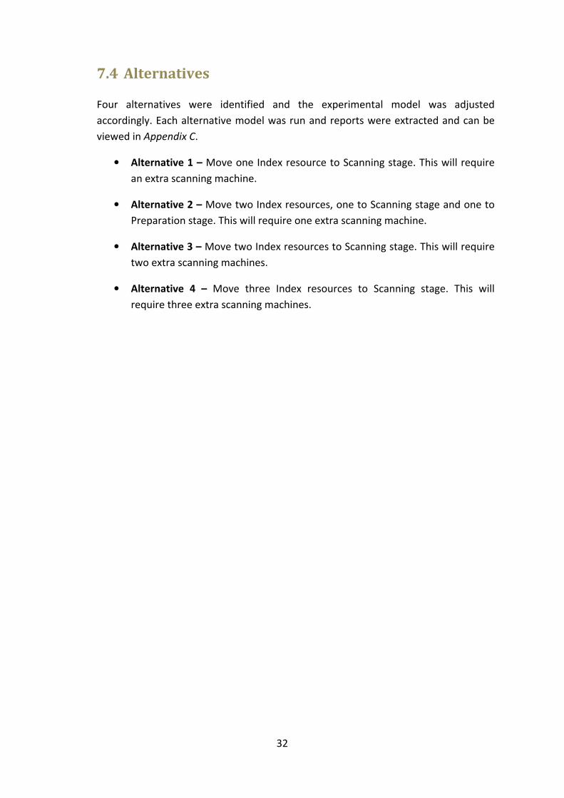
32
7.4 Alternatives
Four alternatives were identified and the experimental model was adjusted
accordingly. Each alternative model was run and reports were extracted and can be
viewed in Appendix C.
• Alternative 1 – Move one Index resource to Scanning stage. This will require
an extra scanning machine.
• Alternative 2 – Move two Index resources, one to Scanning stage and one to
Preparation stage. This will require one extra scanning machine.
• Alternative 3 – Move two Index resources to Scanning stage. This will require
two extra scanning machines.
• Alternative 4 – Move three Index resources to Scanning stage. This will
require three extra scanning machines.

33
8. Evaluation
8.1 Utilisation
As seen in reports (Appendix C), in terms of utilisation, the alternatives improve
progressively from Alternative 1 to Alternative 4. The over-all resource utilisation in
Alternative 4 is 100%.
8.2 Daily Output
Table 7 provides a comparison of the current output (boxes per day) with the other
four alternatives. The improvement order of these alternatives is shown in Figure 10.
Once again, the biggest improvement is represented by Alternative 4.
Table 7: Current and alternative daily outputs per stage
8.3 Queue Lengths
Also shown in the reports, the number of boxes waiting to be processed in front of
every stage becomes less, progressively from Alternative 2 to Alternative 4. The
process also becomes more balanced.
STAGES Current 1 2 3 4
Batch-coding 106 108 106 107 107
Preparation 59 55 65 59 61
Scanning 14 29 24 44 59
Indexing 13 29 23 46 50
ALTERNATIVES

8.4
It is clear that Alternative 4 is the best scenario for
configuration, but
Table 8
parameters used:
Current
Alternative 1
Alternative 2
Alternative 3
Alternative 4
8.4
It is clear that Alternative 4 is the best scenario for
configuration, but
Table 8
parameters used:
Current
Alternative 1
Alternative 2
Alternative 3
Alternative 4
8.4 Total Cost
It is clear that Alternative 4 is the best scenario for
configuration, but
Table 8
parameters used:
•
•
•
Current
Alternative 1
Alternative 2
Alternative 3
Alternative 4
Total Cost
It is clear that Alternative 4 is the best scenario for
configuration, but
Table 8 provides
parameters used:
•
•
•
Current
Alternative 1
Alternative 2
Alternative 3
Alternative 4
Total Cost
It is clear that Alternative 4 is the best scenario for
configuration, but
rovides
parameters used:
Pay Rate
Boxes still to be processed
Cost of new scanner
Alternative 1
Alternative 2
Alternative 3
Alternative 4
Figure
Total Cost
It is clear that Alternative 4 is the best scenario for
configuration, but
rovides
parameters used:
Pay Rate
Boxes still to be processed
Cost of new scanner
Alternative 1
Alternative 2
Alternative 3
Alternative 4
Figure
Total Cost
It is clear that Alternative 4 is the best scenario for
configuration, but
rovides the calculation of
parameters used:
Pay Rate
Boxes still to be processed
Cost of new scanner
Figure
Total Cost
It is clear that Alternative 4 is the best scenario for
configuration, but this alternative requires for the purchasing of three new scanners.
the calculation of
Pay Rate –
Boxes still to be processed
Cost of new scanner
OUTPUT
PER DAY
Figure 10:
Total Cost
It is clear that Alternative 4 is the best scenario for
this alternative requires for the purchasing of three new scanners.
the calculation of
– R 120.00 per operator per day
Boxes still to be processed
Cost of new scanner
Table 8
FINAL
OUTPUT
PER DAY
: Current and alternative daily outputs per stage
It is clear that Alternative 4 is the best scenario for
this alternative requires for the purchasing of three new scanners.
the calculation of
R 120.00 per operator per day
Boxes still to be processed
Cost of new scanner
Table 8
FINAL
OUTPUT
PER DAY
13
29
23
46
50
Current and alternative daily outputs per stage
It is clear that Alternative 4 is the best scenario for
this alternative requires for the purchasing of three new scanners.
the calculation of
R 120.00 per operator per day
Boxes still to be processed
Cost of new scanner
Table 8
FINAL
OUTPUT
PER DAY
Current and alternative daily outputs per stage
It is clear that Alternative 4 is the best scenario for
this alternative requires for the purchasing of three new scanners.
the calculation of
R 120.00 per operator per day
Boxes still to be processed
Cost of new scanner –
Table 8:
OUTPUT
PER DAY
Current and alternative daily outputs per stage
It is clear that Alternative 4 is the best scenario for
this alternative requires for the purchasing of three new scanners.
the calculation of
R 120.00 per operator per day
Boxes still to be processed
– R30,000
: Total cost of alternatives
DAYS TO
COMPLETE
Current and alternative daily outputs per stage
It is clear that Alternative 4 is the best scenario for
this alternative requires for the purchasing of three new scanners.
the calculation of the
R 120.00 per operator per day
Boxes still to be processed
R30,000
Total cost of alternatives
DAYS TO
COMPLETE
79685
35721
45039
22520
20718
34
Current and alternative daily outputs per stage
It is clear that Alternative 4 is the best scenario for
this alternative requires for the purchasing of three new scanners.
the total cost
R 120.00 per operator per day
Boxes still to be processed – 1,035,900
R30,000
Total cost of alternatives
DAYS TO
COMPLETE
79685
35721
45039
22520
20718
34
Current and alternative daily outputs per stage
It is clear that Alternative 4 is the best scenario for
this alternative requires for the purchasing of three new scanners.
total cost
R 120.00 per operator per day
1,035,900
R30,000
Total cost of alternatives
DAYS TO
COMPLETE
79685
35721
45039
22520
20718
Current and alternative daily outputs per stage
It is clear that Alternative 4 is the best scenario for
this alternative requires for the purchasing of three new scanners.
total cost
R 120.00 per operator per day
1,035,900
Total cost of alternatives
DAYS TO
COMPLETE
Current and alternative daily outputs per stage
It is clear that Alternative 4 is the best scenario for
this alternative requires for the purchasing of three new scanners.
total cost
R 120.00 per operator per day
1,035,900
Total cost of alternatives
R
R
R
R
R
Current and alternative daily outputs per stage
It is clear that Alternative 4 is the best scenario for
this alternative requires for the purchasing of three new scanners.
total cost for each alternative.
R 120.00 per operator per day
1,035,900
Total cost of alternatives
LABOUR
COST
143,432,308R
64,297,241R
81,070,435R
40,535,217R
37,292,400R
Current and alternative daily outputs per stage
It is clear that Alternative 4 is the best scenario for
this alternative requires for the purchasing of three new scanners.
for each alternative.
R 120.00 per operator per day
Total cost of alternatives
LABOUR
COST
143,432,308
64,297,241
81,070,435
40,535,217
37,292,400
Current and alternative daily outputs per stage
It is clear that Alternative 4 is the best scenario for
this alternative requires for the purchasing of three new scanners.
for each alternative.
Total cost of alternatives
LABOUR
COST
143,432,308
64,297,241
81,070,435
40,535,217
37,292,400
Current and alternative daily outputs per stage
It is clear that Alternative 4 is the best scenario for the proposed new resource
this alternative requires for the purchasing of three new scanners.
for each alternative.
Total cost of alternatives
LABOUR
143,432,308
64,297,241
81,070,435
40,535,217
37,292,400
Current and alternative daily outputs per stage
the proposed new resource
this alternative requires for the purchasing of three new scanners.
for each alternative.
LABOUR
143,432,308
64,297,241
81,070,435
40,535,217
37,292,400
Current and alternative daily outputs per stage
the proposed new resource
this alternative requires for the purchasing of three new scanners.
for each alternative.
MACHINE
R
R
R
R
R
Current and alternative daily outputs per stage
the proposed new resource
this alternative requires for the purchasing of three new scanners.
for each alternative.
EXTRA
MACHINE
COST
R
30,000R
30,000R
60,000R
90,000R
Current and alternative daily outputs per stage
the proposed new resource
this alternative requires for the purchasing of three new scanners.
for each alternative. Other important
EXTRA
MACHINE
COST
R
30,000
30,000
60,000
90,000
Current and alternative daily outputs per stage
the proposed new resource
this alternative requires for the purchasing of three new scanners.
Other important
EXTRA
MACHINE
COST
-R
30,000
30,000
60,000
90,000
the proposed new resource
this alternative requires for the purchasing of three new scanners.
Other important
MACHINE
30,000
30,000
60,000
90,000
the proposed new resource
this alternative requires for the purchasing of three new scanners.
Other important
143,432,308R
R
R
R
R
the proposed new resource
this alternative requires for the purchasing of three new scanners.
Other important
TOTAL
COST
143,432,308
64,327,241R
81,100,435R
40,595,217R
37,382,400R
the proposed new resource
this alternative requires for the purchasing of three new scanners.
Other important
TOTAL
COST
143,432,308
64,327,241
81,100,435
40,595,217
37,382,400
the proposed new resource
this alternative requires for the purchasing of three new scanners.
Other important
TOTAL
COST
143,432,308
64,327,241
81,100,435
40,595,217
37,382,400
the proposed new resource
this alternative requires for the purchasing of three new scanners.
Other important
TOTAL
143,432,308
64,327,241
81,100,435
40,595,217
37,382,400
TOTAL
143,432,308
64,327,241
81,100,435
40,595,217
37,382,400

35
9. Conclusion
By implementing the resource configuration changes proposed in Alternative 4, an
estimated total savings of R105,000,000 can be expected. The simulation model can now be
used to develop even more alternatives, utilising extra resources, resulting in even bigger
savings.

36
10. Bibliography
[1] Balci, O. (1998). Verification, validation and accreditation. In Medeiros, D., Watson,
E., Carson, J., and Manivannan, M., editors, Proceedings of the 1998 Winter
Simulation Conference, pages 41-48.
[2] Banks, J., Carson II, J. S., and Nelson, B. L. (1996). Discrete-Event System Simulation.
Prentice Hall, New Jersey, second edition.
[3] Banks, J. (2000). Introduction to simulation. In Joines, J. A., Barton, R. R., Kang, K., and
Fishwick, P. A., editors, Proceedings of the 2000 Winter Simulation Conference, pages
9-16.
[4] Carson II, J. S. (2005). Introduction to modelling and simulation. In Kuhl, M. E.,
Steiger, N.M., Armstrong, F. B., and Joines, J. A., editors, Proceedings of the 2005
Winter Simulation Conference, pages 16-23.
[5] Kelton, W. D.,Sadowski, R. P., and Sturrock, D. T. (2007). Simulation with Arena.
McGraw -Hill, New York, fourth edition.
[6] Law, A. M., and Kelton, W. D. (2000). Simulation Modeling and Analysis. McGraw-Hill,
New York, third edition.
[7] Niebel, B. W., and Freivalds, A. (2004). Methods, Standards and Work Design.
McGraw -Hill, New York, eleventh edition.
[8] Oses, N. (2004). Critical issues in the development of component-based discrete
simulation. Simulation Modelling Practice and Theory, 12(7-8):495-514.
[9] Pegden, C. D., Shannon, R. E., and Sadowski, R. P. (1995). Introduction to Simulation
using SIMAN. McGraw-Hill, New York, second edition.
[10] Sargent, R. D. (1998). Verification and validation of simulation models. In Medeiros,
D., Watson, E., Carson, J., and Manivannan, M., editors, Proceedings of the 1998
Winter Simulation Conference, pages 121-130.
[11] Wikipedia (2009). Wikipedia definition of simulation. Available online at
http://en.wikipedia.org/wiki/Simulation. Retrieved on 10 September.

37
Appendix A: Document examples
Control Form Sheet example
During the Batch-coding stage, the ID number is registered onto the system. A control form
is then generated by the information system and printed by the operator. This control form
indicates the registered file’s ID number and that day’s date. An operator has to sign off on
this form after completing the specific stage he/she is responsible for.

38
Time Study example
1 2 3 4 5 6
R W OT NT R W OT NT R W OT NT R W OT NT R W OT NT R W OT NT
95 16.7 16.7 15.9
100 43.3 26.6 26.6
100 70 26.7 26.7
100 98.3 28.3 28.3
100 128 30 30
100 163 35 35
100 197 33.3 33.3
100 220 23.3 23.3
100 252 31.7 31.7
100 282 30 30
100 310 28.3 28.3
100 340 30 30
100 367 26.7 26.7
90 402 35 31.5
Sym W1 W2 OT
A
B
C
D
E
F
G
FINISH
Get box &
remove files
from box.
Register ID
onto system,
produce
printout, sign
& insert into
file.
Gather files,
replace files
into box &
return box.
Setup
Note
Element No. and
Description
6
7
8
9
Total Standard Time (sum standard time for all elements)
10
11
12
Summary
Observer :
Page 1 of 1
Operator : Losipho
Date : 3/7/2009
Operation : Batch-coding
Study No. : 1
Total OT
Cycle
1
2
3
4
5
16.70
% Allowance
Elemental Std Time
15.865
No. Occurences
349.97 35.03
----------
Standard Time
Rating
Total NT
No. Observations
Average NT
32
31.530
1
---------
Time Check Allowance Summary
Remarks: This box containing 12 took
4min 32.8 sec.Total Check Time
349.967
Ineffective Time
Total Recorder Time
12 1
Unaccounted Time
Recording Error %
Personal Needs
Basic Fatigue
Variable Fatigue
Special
Total Allowance %
-----------
3 16 3
15.865 29.164
16.341 33.830 32.476
1 1
TIME STUDY OBSERVATION
FORM:
454.778
16.341 33.830 32.476
1
Effective Time
Starting Time
Elapsed Time
TEBS
TEAF
Finishing Time
Foreign Elements
Rating Check
8
5
3
16
Description
%Synthetic Time
Observed Time

39
Appendix B: Computer Model
Figure 11: Computer model

40
Appendix C: Arena Reports
Current Situation
SCANNING S0.Queue 131.34 73.51 52.9898 203.88 30.0000 222.00
321.00PREPARATION P0.Queue 183.22 106.76 76.8520 293.24 52.0000
INDEXING I0.Queue 0.00 0.00 0.00 0.00 0.00 0.00
81.0000BATCH CODING.Queue 47.1749 26.68 19.8579 74.1336 13.0000
Number Waiting Minimum
Average
Maximum
Average
Minimum
Value
Maximum
ValueAverage Half Width
Queue
20:44:44 Category Overview October 20, 2009
Values Across All Replications
EDPReplications: 5 Time Units: Hours
20:44:44 Category Overview October 20, 2009
Values Across All Replications
EDPReplications: 5 Time Units: Hours
Resource
Usage
Instantaneous Utilization Minimum
Average
Maximum
Average
Minimum
Value
Maximum
ValueAverage Half Width
0.00 1.0000
Batch Coder 1.0000 0.00 1.0000 1.0000 0.00
0.13 0.04221610 0.2462 0.00
1.0000
I1 0.1876 0.13 0.06532925 0.3200
1.0000
I3 0.2008 0.11 0.05251984 0.2700 0.00 1.0000
I2 0.1579
0.00 1.0000
I4 0.1712 0.08 0.07803652 0.2227 0.00
0.12 0.04339951 0.2666 0.00
1.0000
I5 0.1422 0.16 0.00 0.3143
1.0000
P1 1.0000 0.00 1.0000 1.0000 0.00 1.0000
I6 0.1107
0.00 1.0000
P2 1.0000 0.00 1.0000 1.0000 0.00
0.00 1.0000 1.0000 0.00
1.0000
P3 1.0000 0.00 1.0000 1.0000
1.0000
P5 1.0000 0.00 1.0000 1.0000 0.00 1.0000
P4 1.0000
0.00 1.0000
P6 1.0000 0.00 1.0000 1.0000 0.00
0.00 1.0000 1.0000 0.00
1.0000
P7 1.0000 0.00 1.0000 1.0000
1.0000S1 1.0000

41
Alternative 1
SCANNING S0.Queue 43.1038 28.0000 55.0000
PREPARATION P0.Queue 69.9945 45.0000 98.0000
INDEXING I0.Queue 0.00 0.00 0.00
Number Waiting Minimum
Value
Maximum
ValueAverage
BATCH CODING.Queue 19.6369 13.0000 26.0000
Queue
23:15:43 Category Overview October 20, 2009
EDPReplications: 5 Time Units: Hours
S1 1.0000 0.00 1.0000
S2 1.0000 0.00 1.0000
P6 1.0000 0.00 1.0000
P7 1.0000 0.00 1.0000
P4 1.0000 0.00 1.0000
P5 1.0000 0.00 1.0000
P2 1.0000 0.00 1.0000
P3 1.0000 0.00 1.0000
P1 1.0000 0.00 1.0000
I4 0.5807 0.00 1.0000
I5 0.2247 0.00 1.0000
I2 0.3534 0.00 1.0000
I3 0.3182 0.00 1.0000
Batch Coder 1.0000 0.00 1.0000
I1 0.2824 0.00 1.0000
Usage
Instantaneous Utilization Minimum
Value
Maximum
ValueAverage
EDPReplications: 5 Time Units: Hours
Resource
23:15:43 Category Overview October 20, 2009
PREP Boxes Out 55.0000
SCAN Boxes Out 29.0000
CountValue
BATCH Boxes Out 108.00
INDEX Boxes Out 29.0000
Replications: 1 Time Units: Hours
User Specified
Counter
23:15:43 Category Overview October 20, 2009
EDP

42
Alternative 2
SCANNING S0.Queue 51.4640 32.0000 73.0000
PREPARATION P0.Queue 60.0468 39.0000 82.0000
INDEXING I0.Queue 0.00 0.00 0.00
Number Waiting Minimum
Value
Maximum
ValueAverage
BATCH CODING.Queue 20.4740 13.0000 28.0000
Queue
23:24:52 Category Overview October 20, 2009
EDPReplications: 5 Time Units: Hours
S2 1.0000 0.00 1.0000
P8 1.0000 0.00 1.0000
S1 1.0000 0.00 1.0000
P6 1.0000 0.00 1.0000
P7 1.0000 0.00 1.0000
P4 1.0000 0.00 1.0000
P5 1.0000 0.00 1.0000
P2 1.0000 0.00 1.0000
P3 1.0000 0.00 1.0000
P1 1.0000 0.00 1.0000
I4 0.4684 0.00 1.0000
I2 0.4637 0.00 1.0000
I3 0.3867 0.00 1.0000
Batch Coder 1.0000 0.00 1.0000
I1 0.4878 0.00 1.0000
Usage
Instantaneous Utilization Minimum
Value
Maximum
ValueAverage
EDPReplications: 5 Time Units: Hours
Resource
23:24:52 Category Overview October 20, 2009
PREP Boxes Out 65.0000
SCAN Boxes Out 24.0000
Counter
CountValue
BATCH Boxes Out 106.00
INDEX Boxes Out 23.0000
EDPReplications: 5 Time Units: Hours
User Specified
23:24:52 Category Overview October 20, 2009

43
Alternative 3
SCANNING S0.Queue 24.9339 17.0000 32.0000
PREPARATION P0.Queue 69.2182 45.0000 94.0000
INDEXING I0.Queue 0.1726 0.00 3.0000
Number Waiting Minimum
Value
Maximum
ValueAverage
BATCH CODING.Queue 20.0829 13.0000 27.0000
Queue
23:28:12 Category Overview October 20, 2009
EDPReplications: 5 Time Units: Hours
S3 1.0000 0.00 1.0000
S1 1.0000 0.00 1.0000
S2 1.0000 0.00 1.0000
P6 1.0000 0.00 1.0000
P7 1.0000 0.00 1.0000
P4 1.0000 0.00 1.0000
P5 1.0000 0.00 1.0000
P2 1.0000 0.00 1.0000
P3 1.0000 0.00 1.0000
P1 1.0000 0.00 1.0000
I4 0.6888 0.00 1.0000
I2 0.6851 0.00 1.0000
I3 0.7201 0.00 1.0000
Batch Coder 1.0000 0.00 1.0000
I1 0.7685 0.00 1.0000
Usage
Instantaneous Utilization Minimum
Value
Maximum
ValueAverage
EDPReplications: 5 Time Units: Hours
Resource
23:28:12 Category Overview October 20, 2009
23:28:12 Category Overview October 20, 2009
EDPReplications: 5 Time Units: Hours
User Specified
Counter
CountValue
BATCH Boxes Out 107.00
INDEX Boxes Out 46.0000
PREP Boxes Out 59.0000
SCAN Boxes Out 44.0000

44
Alternative 4
SCANNING S0.Queue 9.1447 3.0000 14.0000
PREPARATION P0.Queue 66.4598 44.0000 90.0000
INDEXING I0.Queue 12.4177 7.0000 19.0000
Number Waiting Minimum
Value
Maximum
ValueAverage
BATCH CODING.Queue 19.7093 13.0000 27.0000
Queue
23:57:47 Category Overview October 20, 2009
EDPReplications: 5 Time Units: Hours
S3 1.0000 0.00 1.0000
S4 1.0000 0.00 1.0000
S1 1.0000 0.00 1.0000
S2 1.0000 0.00 1.0000
P6 1.0000 0.00 1.0000
P7 1.0000 0.00 1.0000
P4 1.0000 0.00 1.0000
P5 1.0000 0.00 1.0000
P2 1.0000 0.00 1.0000
P3 1.0000 0.00 1.0000
P1 1.0000 0.00 1.0000
I2 1.0000 0.00 1.0000
I3 1.0000 0.00 1.0000
Batch Coder 1.0000 0.00 1.0000
I1 1.0000 0.00 1.0000
Usage
Instantaneous Utilization Minimum
Value
Maximum
ValueAverage
EDPReplications: 5 Time Units: Hours
Resource
23:57:47 Category Overview October 20, 2009
PREP Boxes Out 61.0000
SCAN Boxes Out 59.0000
CountValue
BATCH Boxes Out 107.00
INDEX Boxes Out 50.0000
Replications: 5 Time Units: Hours
User Specified
Counter
23:57:47 Category Overview October 20, 2009
EDP