improved ray casting generalized implicit surfaces further
TRANSCRIPT
Further GraphicsImproved ray casting
Generalized Implicit Surfaces
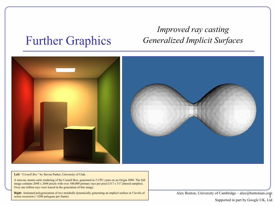
Left: “Cornell Box” by Steven Parker, University of Utah.
A tera-ray monte-carlo rendering of the Cornell Box, generated in 2 CPU years on an Origin 2000. The full image contains 2048 x 2048 pixels with over 100,000 primary rays per pixel (317 x 317 jittered samples). Over one trillion rays were traced in the generation of this image.
Right: Animated polygonization of two metaballs dynamically generating an implicit surface at 5 levels of octree recursion (~3200 polygons per frame) 1
Alex Benton, University of Cambridge – [email protected]
Supported in part by Google UK, Ltd

Great for…● Collision detection between scene
elements● Culling before rendering● Accelerating ray-tracing, -marching
Speed things up!Bounding volumes
A common optimization method for ray-based rendering is the use of bounding volumes.
Nested bounding volumes allow the rapid culling of large portions of geometry
● Test against the bounding volume of the top of the scene graph and then work down.
2

Types of bounding volumesThe goal is to accelerate volumetric tests, such as “does the ray hit the cow?” → speed trumps precision
● choose fast hit testing over accuracy● ‘bboxes’ don’t have to be tight
Axis-aligned bounding boxes● max and min of x/y/z.
Bounding spheres● max of radius from some rough center
Bounding cylinders ● common in early FPS games
3

Bounding volumes in hierarchy
Hierarchies of bounding volumes allow early discarding of rays that won’t hit large parts of the scene.
● Pro: Rays can skip subsections of the hierarchy
● Con: Without spatial coherence ordering the objects in a volume you hit, you’ll still have to hit-test every object
4

Subdivision of space
Split space into cells and list in each cell every object in the scene that overlaps that cell.
● Pro: The ray can skip empty cells
● Con: Depending on cell size, objects may overlap many filled cells or you may waste memory on many empty cells
● Popular for voxelized games (ex: Minecraft)
5

The BSP tree pre-partitions the scene into objects in front of, on, and behind a tree of planes.● This gives an ordering in which to test
scene objects against your ray● When you fire a ray into the scene, you
test all near-side objects before testing far-side objects.
Challenges: ● requires slow pre-processing step● strongly favors static scenes● choice of planes is hard to optimize
Popular acceleration structures:BSP Trees
6
A B
C D E F
A
B
CE
FD

Popular acceleration structures:kd-treesThe kd-tree is a simplification of the BSP Tree data structure ● Space is recursively subdivided by
axis-aligned planes and points on either side of each plane are separated in the tree.
● The kd-tree has O(n log n) insertion time (but this is very optimizable by domain knowledge) and O(n2/3) search time.
● kd-trees don’t suffer from the mathematical slowdowns of BSPs because their planes are always axis-aligned.
Image from Wikipedia, bless their hearts.
7

Popular acceleration structures:Bounding Interval Hierarchies
The Bounding Interval Hierarchy subdivides space around the volumes of objects and shrinks each volume to remove unused space.
● Think of this as a “best-fit” kd-tree● Can be built dynamically as each ray is
fired into the scene
Image from Wächter and Keller’s paper,Instant Ray Tracing: The Bounding Interval Hierarchy, Eurographics (2006)
8

Implicit surfaces Implicit surface modeling(1) is a way to produce very ‘organic’ or ‘bulbous’ surfaces very quickly without subdivision or NURBS.Uses of implicit surface modelling:● Organic forms and nonlinear
shapes● Scientific modeling (electron
orbitals, gravity shells in space, some medical imaging)
● Muscles and joints with skin● Rapid prototyping● CAD/CAM solid geometry
(1) AKA “metaball modeling”, “force functions”, “blobby modeling”… 9

TerminologyIsoclines Isosurfaces
Balázs Csebfalvi, Balázs Tóth, Stefan Bruckner, Meister Eduard GröllerIllumination-Driven Opacity Modulation for Expressive Volume Rendering, Proceedings of Vision, Modeling & Visualization 2012, pages 103-109. November 2012.
Grand Cayon QuadrangleArizona-Coconino Co.7.5 minute series (topographic)Courtesy of National Park Maps (npmaps.com) 10

Implicit surface modelingThe user controls a set of control points or primitives. Each point
generates a field of force, which drops off as a function of distance from the point (like gravity weakening with distance.)
F(r) = “The force at distance r”For any real value , the set of all points in space where the sum of forces
equals is an isosurface: an implicit surface.S = {x∊ℝ3 | ∑pF(|xp|) = }
...or, more prosaically, solve:∑pF(|xp|) - = 0
Force = 2
1
0.5
0.25 ... 11

A few popular force field functions:● “Blobby Molecules” – Jim Blinn
F(r) = a e-br^2
● “Metaballs” – Jim Blinn a(1- 3r2 / b2) 0 ≤ r < b/3
F(r) = (3a/2)(1-r/b)2 b/3 ≤ r < b 0 b ≤ r
● “Soft Objects” – Wyvill & WyvillF(r) = a(1 - 4r6/9b6 + 17r4/9b4 - 22r2 / 9b2)
Force functions
12

Comparison of force functions
13

Rendering implicit surfaces
Several choices:1. Render the surface directly to the GPU
+: Realtime lighting, smooth surfaces, looks great-: Hard to integrate with other objects in scene-: Solve the “intercept surface with ray” problem
2. Convert the surface into a mesh of connected polygons, approximating the surface to a fixed level of precision (“polygon soup”)+: Mesh can be manipulated, interact with scene-: Costly setup costs or runtime framerate hit
14
Rendering implicit surfaceswith Signed Distance Fields
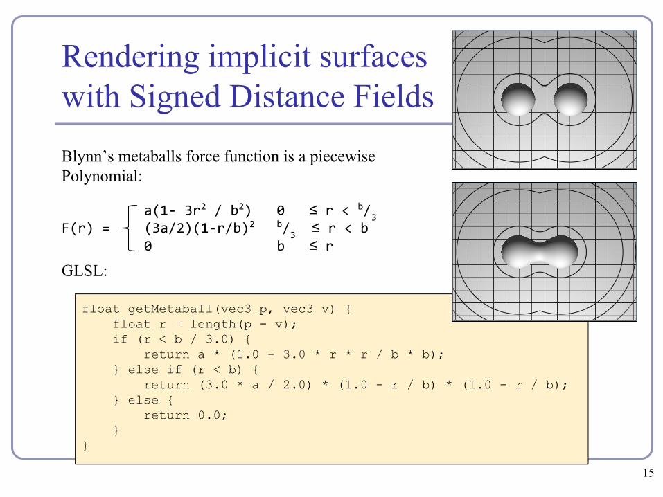
Blynn’s metaballs force function is a piecewise Polynomial:
a(1- 3r2 / b2) 0 ≤ r < b/3
F(r) = (3a/2)(1-r/b)2 b/3 ≤ r < b
0 b ≤ r
GLSL:
float getMetaball(vec3 p, vec3 v) { float r = length(p - v); if (r < b / 3.0) { return a * (1.0 - 3.0 * r * r / b * b); } else if (r < b) { return (3.0 * a / 2.0) * (1.0 - r / b) * (1.0 - r / b); } else { return 0.0; }}
15

Rendering implicit surfaceswith Signed Distance Fields
Let’s use Blynn’s constants: a=1, b=3We want to be able to answer the question, “if F < 0.5, then we’re outside the surface. What is the minimum distance from our current position to F=0.5?”
F = (3a/2)(1-r/b)2
= (3/2)(1-r/3)2
r2 - 6r + (9-6F) = 0r = 3±√(6F)
The square roots yield ± values, but we can discard the half of the polynomial whose r value is >b, leaving us with simply:
r = 3-√(6F)
r = 3-√3
Solve for F = 0.5 → r = 3-√3 = 1.2679529Insight: if we restrict ourselves to metaballs of weight 1, then only Blynn’s second polynomial applies outside the isosurface of F=0.5
16
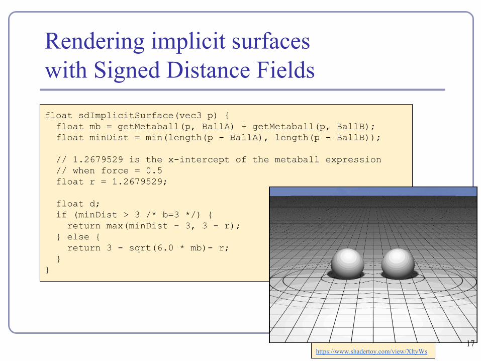
Rendering implicit surfaceswith Signed Distance Fields
float sdImplicitSurface(vec3 p) { float mb = getMetaball(p, BallA) + getMetaball(p, BallB); float minDist = min(length(p - BallA), length(p - BallB));
// 1.2679529 is the x-intercept of the metaball expression // when force = 0.5 float r = 1.2679529;
float d; if (minDist > 3 /* b=3 */) { return max(minDist - 3, 3 - r); } else { return 3 - sqrt(6.0 * mb)- r; }}
https://www.shadertoy.com/view/XltyWs 17

Image credit: J W Laprairie, Mark & Hamilton, Howard. (2018). Isovox: A Brick-Octree Approach to Indirect Visualization
Rendering implicit surfaces with polygons
An octree is a recursive subdivision of space which “homes in” on the surface, from larger to finer detail. ● An octree encloses a cubical volume in space.
You evaluate the force function F(v) at each vertex v of the cube.
● As the octree subdivides and splits into smaller octrees, only the octrees which contain some of the surface are processed; empty octrees are discarded.
18

Polygonizing the surface
To display a set of octrees, convert the octrees into polygons.
● If some corners are “hot” (above the force limit) and others are “cold” (below the force limit) then the isosurface must cross the cube edges in between.
● The set of midpoints of adjacent crossed edges forms one or more rings, which can be triangulated. The normal is known from the hot/cold direction on the edges.
To refine the polygonization, subdivide recursively; discard any child whose vertices are all hot or all cold.
19

Polygonizing the surface
Recursive subdivision (on a quadtree):
20

Polygonizing the surfaceThere are fifteen possible configurations (up to symmetry) of hot/cold vertices in the cube. →● With rotations, that’s 256 cases.
Beware: there are ambiguous cases in the polygonization which must be addressed separately. ↓
Images courtesy of Diane Lingrand
21
Polygonizing the surface
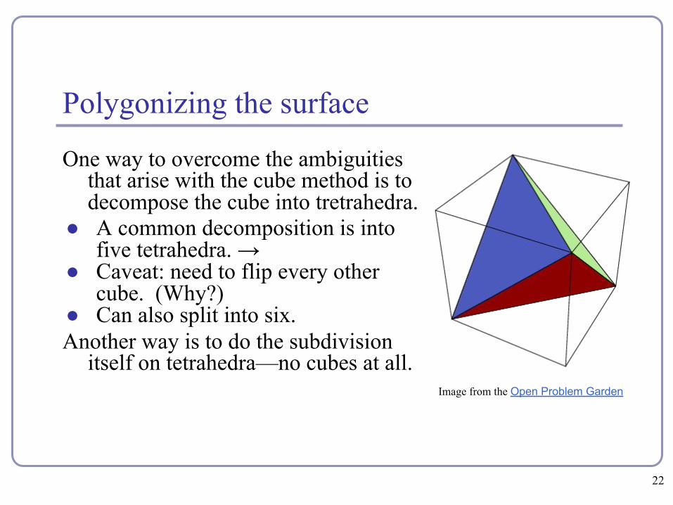
One way to overcome the ambiguities that arise with the cube method is to decompose the cube into tretrahedra.
● A common decomposition is into five tetrahedra. →
● Caveat: need to flip every other cube. (Why?)
● Can also split into six.Another way is to do the subdivision
itself on tetrahedra—no cubes at all.Image from the Open Problem Garden
22

Smoothing the polygonization
Improved edge vertices● The naïve implementation builds polygons whose vertices are the midpoints
of the edges which lie between hot and cold vertices.● The vertices of the implicit surface can be more closely approximated by
points linearly interpolated along the edges of the cube by the weights of the relative values of the force function.● t = (0.5 - F(P1)) / (F(P2) - F(P1))● P = P1 + t (P2 - P1)
Same force points 23

Marching cubesAn alternative to octrees if you only want to compute the final stage is the marching cubes algorithm (Lorensen & Cline, 1985):● Fire a ray from any point known to be
inside the surface.● Using Newton’s method or binary search,
find where the ray crosses the surface. ● Newton: derivative estimated from discrete
local sampling● There may be many crossings
● Drop a cube around the intersection point: it will have some vertices hot, some cold.
● While there exists a cube which has at least one hot vertex and at least one cold vertex on a side and no neighbor on that side, create a neighboring cube on that side. Repeat.
Marching cubes is common in medical imaging such as MRI scans.It was first demonstrated (and patented!) by researchers at GE in 1984, modeling a human spine.
24
ReferencesImplicit modelling:D. Ricci, A Constructive Geometry for Computer Graphics, Computer Journal, May 1973J Bloomenthal, Polygonization of Implicit Surfaces, Computer Aided Geometric Design,
Issue 5, 1988B Wyvill, C McPheeters, G Wyvill, Soft Objects, Advanced Computer Graphics (Proc. CG
Tokyo 1986)B Wyvill, C McPheeters, G Wyvill, Animating Soft Objects, The Visual Computer, Issue 4
1986http://astronomy.swin.edu.au/~pbourke/modelling/implicitsurf/http://www.cs.berkeley.edu/~job/Papers/turk-2002-MIS.pdfhttp://www.unchainedgeometry.com/jbloom/papers/interactive.pdfhttp://www-courses.cs.uiuc.edu/~cs319/polygonization.pdf
25