Wireless Sensor Network, 2017, 9, 73-86 http://www.scirp.org/journal/wsn

ISSN Online: 1945-3086 ISSN Print: 1945-3078

DOI: 10.4236/wsn.2017.92004 February 21, 2017

Improved Self-Pruning for Broadcasting in Ad Hoc Wireless Networks

Raqeebir Rab1, Shaheed Ahmed Dewan Sagar1, Nazmus Sakib1, Ahasanul Haque1, Majedul Islam1, Ashikur Rahman2

1Department of Computer Science and Engineering, Ahsanullah University of Science and Technology, Dhaka, Bangladesh 2Department of Computer Science and Engineering, Bangladesh University of Engineering and Technology (BUET), Dhaka, Bangladesh

Abstract Reducing number of forwarding nodes is the main focus of any broadcasting algorithm designed for ad-hoc wireless networks. All reliable broadcasting techniques can be broadly classified under proactive and reactive approaches. In proactive approach, a node selects a subset of its neighbors as forwarding node and announces the forwarding node list in the packet header during broadcast. On the other hand, no such forwarding list is generated in reactive approach. Rather, a node (cognitively) determines by itself whether to forward the packet or not based on neighbor information. Dominant pruning and Self- pruning are two example techniques that fall under proactive and reactive ap-proach respectively. Between the two methods, dominant pruning shows bet-ter performance than self-pruning in reducing number of forwarding nodes as they work with extended neighbor knowledge. However, appended forward-ing node list increases message overhead and consumes more bandwidth. As a result, the approach becomes non-scalable in large networks. In this paper, we propose a reactive broadcasting technique based on self-pruning. The pro-posed approach dubbed as “Improved Self-pruning based Broadcasting (ISB)” algorithm completes the broadcast with smaller packet header (i.e., with no overhead) but uses extended neighbor knowledge. Simulation results show that ISB outperforms dominant pruning and self-pruning. Furthermore, as the network gets more spread and denser, ISB works remarkably well.

Keywords Broadcasting, Pruning, Forwarding Set, Heuristics

1. Introduction

In recent years, Mobile Ad Hoc Networks (MANETs) have received much atten-

How to cite this paper: Rab, R., Sagar, S.A.D., Sakib, N., Haque, A., Islam, M. and Rahman, A. (2017) Improved Self-Pruning for Broadcasting in Ad Hoc Wireless Net-works. Wireless Sensor Network, 9, 73-86. https://doi.org/10.4236/wsn.2017.92004 Received: December 28, 2016 Accepted: February 18, 2017 Published: February 21, 2017 Copyright © 2017 by authors and Scientific Research Publishing Inc. This work is licensed under the Creative Commons Attribution International License (CC BY 4.0). http://creativecommons.org/licenses/by/4.0/

Open Access

R. Rab et al.

74

tion from the research community for designing wireless networks. A wireless ad hoc network [1] is a collection of two or more devices which creates self- generated mobile networks. For such networks, no pre-existing infrastructure is needed and every node works as a router where they communicate in a peer-to- peer fashion. It is basically a temporary network which is formed for a specific purpose. After the purpose is served, the network is deformed automatically. Ad Hoc Networks are more adaptive and more reconfigurable.

The main issue with an ad hoc network is that the network topology is never static; node mobility is very high; and resources (i.e., available bandwidth) are very limited. In order to tackle high mobility, broadcasting is more frequently used in ad hoc networks. As the wireless medium is inherently broadcast, the efficiency of any broadcasting technique relies on effective forwarding me- chanism. In low mobility scenario, a tree-based approach such as minimal connected dominating set (MCDS) [2] yields a better result as this scheme uses minimum resources. But in a highly mobile environment, flooding techniques [3] have been proven effective as it generally ensures full coverage throughout the topology.

Simple flooding discussed in [2] [4] proposes an algorithm which starts by a source node broadcasting a packet to all its neighbors. Each neighbor rebroad-casts the packets until all the nodes in the topology receive the packet. Simple flooding ensures reliable broadcasting but it causes redundancy, contention and collision which are known as broadcast storm problem [4]. Although all the nodes are supposed to receive the broadcast packet when flooding is used, only a fraction of nodes eventually receive the broadcast in reality [4] due to the noto-rious broadcast storm. Selecting intermediate forwarding nodes intelligently can significantly reduce the broadcast storm problem.

Several techniques have been proposed to choose the intermediate forwarding nodes efficiently [5] [6] [7] [8]. All these solutions utilize neighborhood infor-mation to reduce the number of redundant packets. We broadly classify all those attempts into two categories: 1) Reactive and 2) Proactive schemes. By a reactive scheme, a copy of the broadcast packet is always intended for all the nodes that can receive it. Then, it is up to the receiving node to decide whether the packet should be re-broadcast further down the broadcast chain. In contrast, with a proactive solution, the transmitting node indicates (by providing a forwarding list in the header) which of its neighbors are supposed to re-broadcast the pack-et. Then, having received such a packet, a node essentially knows its role. If it has been chosen as one of the forwarders, it is required to produce a similar for-warding list among its own neighbors and rebroadcast replacing the forwarding list with the newly constructed one.

With the reactive approach, a receiving node decides to rebroadcast the packet only if it concludes that its retransmission is going to cover new nodes, i.e., ones that have not been already covered by the received packet. For example, with self- pruning [6], a re-broadcasting node includes the list of its neighbors in the packet header. A receiving node consults that list and retransmits the packet only if its

R. Rab et al.

75

own set of neighbors includes nodes that are not mentioned in the packet’s list. In a proactive scheme, a transmitting node selecting the forwarders from

among its neighbors may use such criteria as node degree, power level, coverage area, etc. Examples of such solutions include dominant pruning [6], partial dominant pruning, and total dominant pruning [7]. Dominant pruning (DP) exploits 2-hop neighbor information. Each node maintains a subset of its one- hop neighbors (called forward list) whose retransmissions will cover all nodes located two hops away from the node. The forward list is passed in the header of every packet re-transmitted by the node. Total dominant pruning (TDP) and Partial dominant pruning (PDP) attempt to reduce the redundancy of DP by creatively eliminating some nodes from the forward list.

Among the two approaches proactive protocols show better performance in terms of reducing the number of forwarding nodes. However, in proactive tech-niques the packet size is substantially larger than the reactive techniques as it sends the list of next-hop forwarding nodes in the packet header. Putting for-warding-list in the header is always a non-scalable solution as it grows with the network size. Another problem with the proactive approaches is they are poor in handling dynamic topology. As in the reactive approaches receiving nodes have to decide whether it wants to be a forwarding node or not, when new nodes are added to the topology those nodes are automatically accounted for. On the other hand, proactive approaches send the next-hop forwarding node in the packet header, so there is no guarantee that the newly added nodes would be imme-diately reflected in the forwarding node lists. Moreover, the packet size is smaller and the execution time is faster in reactive techniques.

In this paper, we propose an improved self-pruning broadcasting technique which overcomes the drawback of the traditional self-pruning. In the proposed technique, each node makes its forwarding decision based on three hop neighbor knowledge. With the extended neighbor information improved self-pruning performs exceedingly better than traditional self-pruning and dominant pruning and generates lower number of forwarding nodes. As it is an improved version of the self-pruning, it inherits all benefits of the reactive broadcast protocols. During transmission the packet size remains minimal and no extra overhead is generated in the packet header. To validate efficiency of our heuristics we com-pare the performance with other three techniques using extensive simulations.

The organization of the paper is as follow. This section introduces the prob-lem that we solve and summarizes our contribution. Section 2 describes the re-lated works in this direction. Section 3 discusses self-pruning and dominant pruning in details. We introduce our new improved self-pruning in Section 1. Section 4 presents the simulation results to validate the effectiveness of newly proposed heuristic. Finally, we conclude the paper with probable future works in Section 7.

2. Related Works

The redundancy of naive flooding was studied in [4], where the broadcast storm

R. Rab et al.

76

problem was identified. As a way out, the authors suggested a probabilistic ap-proach driven by several types of heuristics, including counter-based, distance- based, location-based, and cluster-based schemes. All those solutions mainly differ on two issues: how a node can assess the redundancy of a retransmission, and how the nodes can collectively utilize such assessments. The main problem of all those algorithms is that they only yield a probabilistic coverage of any broadcast operation and only a fraction of nodes receives the broadcast.

Lim and Kim [6] proved that building a minimum flooding tree is equivalent to finding a minimum connected dominating set (MCDS), which is an NP- complete problem. In [6], they also suggested a few efficient forwarding schemes for broadcasting as well as multicasting, notably self-pruning and dominant pruning. With self-pruning, each node only has to be aware of its one-hop neighbors, which is accomplished via periodic HELLO messages. For dominant pruning, based on 2-hop neighbor information. the HELLO messages are sent with the TTL (time to live) of 2, which means that each of them is re-broadcast once.

Peng et al. [5] presented a modification of the self-pruning algorithm named SBA (for scalable broadcast algorithm). The scheme imposes randomized delays before retransmissions. Similar to [6], a node does not rebroadcast its copy of the packet, if the copies received during the waiting time appear to have covered all its neighbors. The performance of this scheme turns out to be very sensitive to the length of the waiting period.

In [9], Rahman and Gburzynski introduced a generic broadcast algorithm based on delaying the retransmission in order to collect more information about the neighborhood. The proper selection of defer time plays a significant role in the performance of the proposed schemes. Except for the most naive probabi- listic criterion, it is natural to expect that the longer the defer time, the more information is likely to reach the node before it is forced to make the decision. This demonstrates the trade-off between the latency and redundancy of the broadcast operation.

Total dominant pruning (TDP) and partial dominant pruning (PDP) pro- posed in [7] appear to make the most efficient use of neighborhood information. With TDP, 2-hop neighborhood information from the immediate sender is included in the header of every broadcast packet. A node receiving such a packet builds its forward list based on that information. The main drawback of TDP is that it requires high bandwidth (and long packets), at least in those scenarios where the neighborhoods tend to be large.

3. Self-Pruning and Dominant Pruning

In this section we review the self-pruning and dominant pruning techniques in detail proposed by Lim and Kim [8].

Let ( )N u be the set of all one-hop neighbors of u . By ( ) ( ) ( ) ( ){ }2N u v v N u z v N z z N u= ∈ ∃ ∈ ∈ ∨ ∧ we shall denote the set of all

one-hop and two-hop neighbors of u .

R. Rab et al.

77

In self-pruning and dominant pruning [8] it is assumed that each node knows its adjacent nodes. This assumption is not unreasonable as most of the routing protocols designed for wireless ad hoc networks are based on this assumption In order derive nighborhood information, all nodes continuously emits who am I packet to inform the adjacent nodes about their presence. When sender node sends the packet it also piggybacks its neighbor list with the packet, thus it becomes easy to compute ( )2N u by the other nodes of ( )N u .

In self-pruning, upon receiving a packet, a node decides by itself whether it is going to be a forwarding node or not. If ( )N I is the neighbors of the sender node I then the receiver node J is going to be a forwarding node if the set

( ) ( )N J N I− is nonempty. Otherwise the receiver node drops the packet without forwarding further down the broadcast chain.

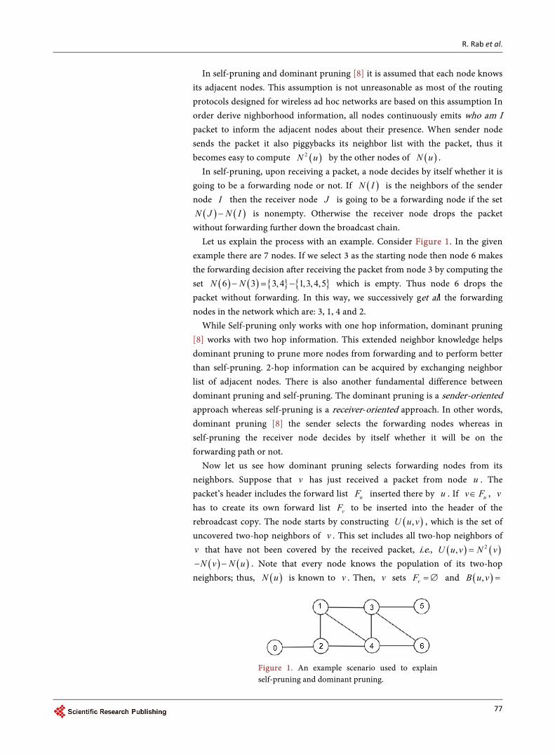
Let us explain the process with an example. Consider Figure 1. In the given example there are 7 nodes. If we select 3 as the starting node then node 6 makes the forwarding decision after receiving the packet from node 3 by computing the set ( ) ( ) { } { }6 3 3,4 1,3,4,5N N− = − which is empty. Thus node 6 drops the packet without forwarding. In this way, we successively get all the forwarding nodes in the network which are: 3, 1, 4 and 2.

While Self-pruning only works with one hop information, dominant pruning [8] works with two hop information. This extended neighbor knowledge helps dominant pruning to prune more nodes from forwarding and to perform better than self-pruning. 2-hop information can be acquired by exchanging neighbor list of adjacent nodes. There is also another fundamental difference between dominant pruning and self-pruning. The dominant pruning is a sender-oriented approach whereas self-pruning is a receiver-oriented approach. In other words, dominant pruning [8] the sender selects the forwarding nodes whereas in self-pruning the receiver node decides by itself whether it will be on the forwarding path or not.

Now let us see how dominant pruning selects forwarding nodes from its neighbors. Suppose that v has just received a packet from node u . The packet’s header includes the forward list uF inserted there by u . If uv F∈ , v has to create its own forward list vF to be inserted into the header of the rebroadcast copy. The node starts by constructing ( ),U u v , which is the set of uncovered two-hop neighbors of v . This set includes all two-hop neighbors of v that have not been covered by the received packet, i.e., ( ) ( )2,U u v N v=

( ) ( )N v N u− − . Note that every node knows the population of its two-hop neighbors; thus, ( )N u is known to v . Then, v sets vF = ∅ and ( ),B u v =

Figure 1. An example scenario used to explain self-pruning and dominant pruning.

R. Rab et al.

78

( ) ( )N v N u− . The set ( ),B u v represents those neighbors of v which are possible candidates for inclusion in vF . Then, in each iteration, v selects a neighbor ( ),w B u v∈ , such that w is not in vF and the list of neighbors of w covers the maximum number of nodes in ( ),U u v , i.e., ( ) ( ),N w U u v∩ is maximized. Next v includes w in vF and sets ( ) ( ) ( ), ,U u v U u v N w= − . The iterations continue for as long as ( ),U u v becomes nonempty or no more progress can be accomplished (i.e., there is no way to further improve the coverage).

Let us illustrate forwarding list creation in dominant pruning by the same example scenario of Figure 1. Suppose node 3 is the broadcast initiator. For node 3, ( ) { }2 3 1,2,3,4,5,6N = , ( ) { }3 1,3, 4,5,6N = . So ( ) ( ) ( ) { } { } { }2,3 3 2 1,2,3,4,5,6 1,3,4,5,6 2U N N∅ = − −∅ = − = . And ( ) ( ) { },3 3 1,4,5,6B N∅ = −∅ = . Thus it needs to choose a node from the set ( ),3B ∅ (which is { }1,4,5,6 ) to cover nodes in ( ),3U ∅ (which is { }2 ). It

can pick either node 1 or node 4 to cover node 2.

4. Improved Self-Pruning Algorithm

In this section we describe a new Improved Self-pruning based Broadcasting (ISB) algorithm. The main idea of the algorithm is as follows.

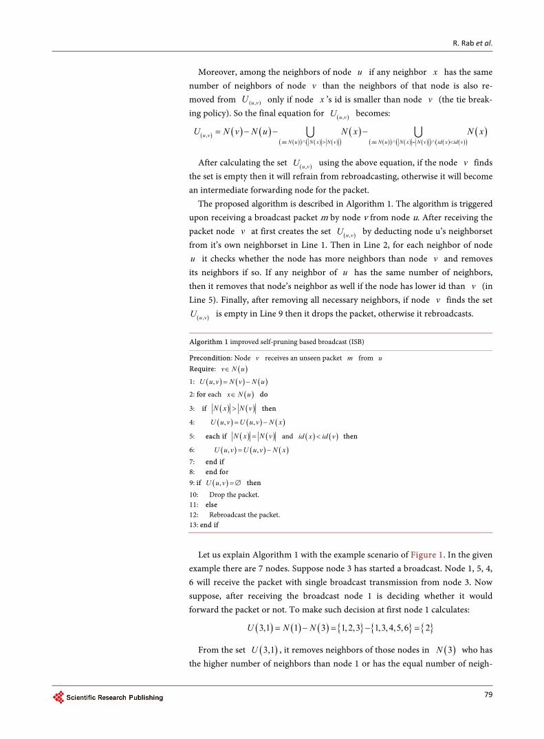
Like self-pruning, when a node receives a broadcast packet it decides by itself whether to rebroadcast the packet or not based on its neighborhood information. For example, consider the scenario of Figure 2. In this scenario, a node v has just received a broadcast packet from node u . To make the rebroadcasting decision, the node v at first removes the neighbors of node u denoted by

( )N u from its own neighborset ( )N v . In other words, it creates a set ( ),u vU using the following equation:

( ) ( ) ( ),u vU N v N u= −

Then from the set ( ),u vU , it removes the neighbors of those nodes who are the neighbor of source node u and have more neighbors than node v , i.e.,

( ) ( ) ( )( )( ) ( ) ( )( )

( ),u vx N u N x N v

U N v N u N x∈ >

= − − ∪∧

Figure 2. Illustrating improved self-pruning algorithm.

R. Rab et al.

79

Moreover, among the neighbors of node u if any neighbor x has the same number of neighbors of node v than the neighbors of that node is also re- moved from ),( vuU only if node x ’s id is smaller than node v (the tie break- ing policy). So the final equation for ( ),u vU becomes:

( ) ( ) ( )( )( ) ( ) ( )( )

( )( )( ) ( ) ( )( ) ( ) ( )( )

( ),u vx N u N x N v x N u N x N v id x id v

U N v N u N x N x∈ > ∈ = <

= − − −∪ ∪∧ ∧ ∧

After calculating the set ( ),u vU using the above equation, if the node v finds the set is empty then it will refrain from rebroadcasting, otherwise it will become an intermediate forwarding node for the packet.

The proposed algorithm is described in Algorithm 1. The algorithm is triggered upon receiving a broadcast packet m by node v from node u. After receiving the packet node v at first creates the set ( ),u vU by deducting node u’s neighborset from it’s own neighborset in Line 1. Then in Line 2, for each neighbor of node u it checks whether the node has more neighbors than node v and removes its neighbors if so. If any neighbor of u has the same number of neighbors, then it removes that node’s neighbor as well if the node has lower id than v (in Line 5). Finally, after removing all necessary neighbors, if node v finds the set

( ),u vU is empty in Line 9 then it drops the packet, otherwise it rebroadcasts.

Algorithm 1 improved self-pruning based broadcast (ISB)

Precondition: Node v receives an unseen packet m from u Require: ( )v N u∈

1: ( ) ( ) ( ),U u v N v N u= −

2: for each ( )x N u∈ do

3: if ( ) ( )N x N v> then

4: ( ) ( ) ( ), ,U u v U u v N x= −

5: each if ( ) ( )N x N v= and ( ) ( )id x id v< then

6: ( ) ( ) ( ), ,U u v U u v N x= − 7: end if 8: end for 9: if ( ),U u v =∅ then 10: Drop the packet. 11: else 12: Rebroadcast the packet. 13: end if

Let us explain Algorithm 1 with the example scenario of Figure 1. In the given

example there are 7 nodes. Suppose node 3 has started a broadcast. Node 1, 5, 4, 6 will receive the packet with single broadcast transmission from node 3. Now suppose, after receiving the broadcast node 1 is deciding whether it would forward the packet or not. To make such decision at first node 1 calculates:

( ) ( ) ( ) { } { } { }3,1 1 3 1,2,3 1,3,4,5,6 2U N N= − = − =

From the set ( )3,1U , it removes neighbors of those nodes in ( )3N who has the higher number of neighbors than node 1 or has the equal number of neigh-

R. Rab et al.

80

bors but lower id value than node 1. Only node 4 has the higher number of neighbors. so it removes ( )4N and after removal the ( )3,1U becomes ( ) ( ) { } { }3,1 4 2 1,2,3,4,6U N− = − = ∅ . So node 1 will not forward the packet.

When all the nodes run the improved self-pruning algorithm successively in this topology we get only node 3, 4 and 2 as the forwarding nodes.

5. Example

In this section we provide an example scenario to illustrate the benefit of using improved self-pruning algorithm.

Figure 3 shows an example network with 12 nodes. Suppose node 6 has initiated a broadcast. The neighbor information of the aforementioned topology is shown in Table 1. For determining a list of forwarding nodes in self-pruning, dominant pruning and improved self-pruning algorithms this sample scenario will be used next. Note that, for any node v, the set ( )N v includes the node v.

Figure 3. A random example scenario of 12 nodes.

Table 1. Detail analysis of example scenario in Figure 3.

v ( )N v ( )( )N N v

1 { }1,2,5 { }1,2,3,5,6,7,9

2 { }1,2,3,6,7 { }1,2,3,4,5,6,7,8,9,11

3 { }2,3,4 { }1, 2,3, 4,6,7,8

4 { }3,4,7,8 { }2,3, 4,67,8,11,12

5 { }1,5,6,9 { }1,2,5,6,7,9,10

6 { }2,5,6,7,9 { }1,2,3,4,5,6,7,8,9,10,11

7 { }2,4,6,7,8,11 { }1,2,3,4,5,6,7,8,9,10,11,12

8 { }4,7,8,12 { }2,3,4,6,7,8,11,12

9 { }5,6,9,10 { }1,2,5,6,7,9,10,11

10 { }9,10,11 { }5,6,7,9,10,11,12

11 { }7,10,11,12 { }2,4,6,7,8,9,10,11,12

12 { }8,11,12 { }4,7,8,10,11,12

R. Rab et al.

81

First of all, we will determine the list of forwarding nodes in self-pruning algorithm. From node 6, node 2, 5, 7 and 9 will receive the broadcast. After receiving the broadcast, node 2 will check if the set ( ) ( )2 6N N− is empty or not. If the set is empty then it will not be a forwarding node, otherwise it will forward. Now, ( ) { }6 2,5,6,7,9N = and ( ) { }2 1,2,3,6,7N = so ( ) ( )2 6N N− is { } { } { }1,2,3,6,7 2,5,6,7,9 1,2,3− = . As it is non-empty, node 2 will be a for- warding node. In the same way, for all other nodes we can sequentially deter- mine which of the other nodes will be forwarding nodes. Table 1 and Table 2 show the complete analysis. After analysis, we can see that all the nodes except node 12 will forward the packet. Thus self-pruning will need 11 forwarding to complete the broadcast.

Now let us see how dominant pruning will perform. Again consider node 6 is the starting node. Now as we know dominant pruning uses two hop neighbor information and transmits the forwarding list with its packet. Now let us find out the forwarding list of node 6. ( ) ( )( ) ( ) ( ) { },6 6 6 1,3,4,8,10,12U N N N N∅ = − ∅ − = and ( ) ( ) { },6 6 2,5,6,7,9B N∅ = −∅ = . Therefore, the forwarding list for node 6 will

be { }7,2,9 . Similarly, we can find a complete list of forwarding node list for all other nodes. Table 3 shows the complete analysis. Nodes 6,7,2,9,11,3, and 10 will forward the packet, comprising a total of 7 forwarding to complete the broadcast.

Finally, we show the number of forwarding’s using the proposed improved self-pruning algorithm (ISB). For ISB, as node 6 is the starting node, nodes 2,5,7,9 will get the packet with the single transmission from node 6. Then to decide whether node 2 will forward or not node 2 would calculate the set ( ) ( ) ( ) { } { } { }6, 2 2 6 1,2,3,6,7 2,5,6,7,9 1,3U N N= − = − = . From the set U(6,2)

Table 2. Detail analysis of self-pruning algorithm for the scenario in Figure 3.

u v ( ) ( )N v N u− Forward?

∅ 6 { }2,5,7,9 Yes

6 2 ( ) ( ) { }2 6 1,3N N− = Yes

6 5 ( ) ( ) { }5 6 1N N− = Yes

6 7 ( ) ( ) { }7 6 4,8,11N N− = Yes

6 9 ( ) ( ) { }9 6 10N N− = Yes

2 1 ( ) ( ) { }1 2 1N N− = Yes

2 3 ( ) ( ) { }3 2 4N N− = Yes

7 4 ( ) ( ) { }4 7 3N N− = Yes

7 8 ( ) ( ) { }8 7 12N N− = Yes

7 11 ( ) ( ) { }11 7 10,12N N− = Yes

9 10 ( ) ( ) { }10 9 11N N− = Yes

R. Rab et al.

82

Table 3. Detail analysis of Dominant Pruning algorithm for the scenario in Figure 3.

u v ( ),U u v ( ),B u v ( )F v

∅ 6 { }1,3,4,8,10,11 { }2,5,7,9 { }7,2,9

6 7 { }1,3,10,12 { }4,8,11 { }11,4

6 2 { }4,8,11 { }1,3 { }3

6 9 { }1,11 { }10 { }10

7 11 { }9 { }10,12 { }10

7 4 { }12 { }3 ∅

2 3 { }8 { }4 { }4

9 10 { }7,12 { }11 { }11

now the neighbor of the nodes in ( )6N will be removed from ( )2N who has more neighbors than node 2 or has the same number of neighbors but lower id than node 2. With this conditions node 7 will be selected as only node 7 has higher number of neighbors than node 2. All other nodes in ( )6N have less neighbors of neighbors than node 2. So, ( ) ( ) ( ) { }6,2 6,2 7 1,3U U N= − = − { } { }2,4,6,7,8,11 1,3= which is non-empty. Thus, node 2 will be a forwarding node. Table 4 shows the complete analysis. Nodes 6, 7, 2, 9, 8 and 10 will forward the packet, comprising a total of 6 forwarding to complete the broad- cast.

In summary, the self-pruning, dominant pruning and improved self-pruning will incur 11, 7 and 6 forwarding respectively to complete the broadcast in the example scenario of Figure 4. The optimum number of broadcasts is 5 for this network because if only 6, 7, 2, 9, 8 forward the packet then all the nodes in the network would receive the packet. Thus, the improved self-pruning exhibits the best performance among the three algorithms we discussed, incurring only one extra forwarding compared to the optimal.

6. Performance

To see the effectiveness of the improved self-pruning, we implement the algo-rithm along with the self-pruning, and dominant pruning algorithm. The simu-lation code-base was built using Java programming language. Finally we perform a comparative analysis based on the simulation results.

Simulation environment. To evaluate the performance, we simulate randomly deployed networks of 100 - 500 nodes over a fixed 625 m × 625 m square region. Depending on the node density, the random scenarios can be broadly catego-rized into sparse, moderately dense and dense networks. The maximum trans-mission radius is limited between 125 m to 225 m. The number of forwarding node is used as performance metrics.

Less is better, i.e., lower number of forwarding nodes indicate better perfor- mance.

R. Rab et al.

83

Table 4. Detail analysis of Improved Self-pruning algorithm for the scenario in Figure 4.

u v ( ),U u v Forward?

∅ 6 { }2,5,7,9 Yes

6 2 ( ) ( ) ( ) { }2 6 7 1,3N N N− − = Yes

6 7 ( ) ( ) { }7 6 4,8,11N N− = Yes

6 5 ( ) ( ) ( ) ( )5 6 7 2N N N N− − − =∅ No

6 9 ( ) ( ) ( ) ( ) ( ) { }9 6 7 2 5 10N N N N N− − − − = Yes

2 1 ( ) ( ) ( ) ( )1 2 6 7N N N N− − − =∅ No

2 3 ( ) ( ) ( ) ( ) ( )3 2 6 7 1N N N N N− − − − =∅ No

7 4 ( ) ( ) ( ) ( )4 7 6 2N N N N− − =∅ No

7 8 ( ) ( ) ( ) ( ) { }8 7 6 4 12N N N N− − = Yes

7 11 ( ) ( ) ( ) ( ) ( ) ( )11 7 6 2 4 8N N N N N N− − − =∅ No

9 10 ( ) ( ) ( ) ( ) { }10 9 6 5 11N N N N− − − = Yes

Figure 4. Performance comparidon in sparse networks.

Effect of transmission range. Figure 4 shows the effect of transmission range

on sparse networks. For these scenarios we have run simulations for 100 nodes having homogeneous transmission range between 125 m to 225 m. We have generated 10 different scenarios for each of the transmission ranges and took the mean value of the number of forwarding nodes for the self-pruning, dominant pruning and improved self-pruning. Only 20 - 40 nodes forward the packets on the average to complete a broadcast in the network for improved self-pruning. Dominant pruning causes 50 - 60 nodes to forward whereas the self-pruning shows worst performance needing 75 - 85 nodes to forward. We can also see that the improved self-pruning generates better results for all transmission ranges using least number of forwarding nodes to complete a broadcast.

R. Rab et al.

84

From Figure 5 it is also evident that, as the transmission range increases the performance of the self-pruning deteriorates and the performance of dominant and improved self-pruning gets better. With larger transmission ranges each node has more neighbors in its transmission range compared to short trans- mission ranges. Consequently, there is a high probability that a nodes neighbors are already covered by other node’s transmissions. As dominant pruning and improved self-pruning utilizes two hop neighbor information they can easily detect those redundant transmissions and inhibit those nodes from forwarding the packet whose neighbors already receive the packet from other neighbors. As self-pruning only uses 1 hop information, it can not detect such redundant trans- missions and causes more forwarding.

In order to generate moderately dense networks (Figure 6), we have increased the number of nodes to 350 within the same deployment area of 625 m 625 m× . Transmission ranges are similar and the results reported are again average of 10

Figure 5. Performance simulation in a moderately dense network.

Figure 6. Performance simulation in a dense network.

R. Rab et al.

85

random samples. Again, improved self-pruning outperforms other two tech- niques with similar performance trend with the increased transmission ranges.

Dense networks (Figure 6) were generated by increasing the number of nodes to 500 while keeping all other settings similar. Needless to say that, improved self- pruning shows most optimization incurring least number of forwarding nodes.

Effect of node density. Figure 7 shows the effect of node density on the per- formance of the three algorithms. Here we have set the transmission range fixed to 150 m but each scenarios has different node counts ranging from 100 to 500 nodes.

From the graph it is clearly evident that as the number of nodes in the net-work increases the efficiency of self-pruning and dominant pruning drops sig-nificantly. On the other hand, improved self-pruning performs substantially better than the other two. Although the number of forwarding nodes linearly in-creases with the node number for the self-pruning and the dominant pruning algorithms, this growth is almost negligible for improved self-pruning.

In summary, the performance of improved self-pruning based broadcasting (ISB) algorithm increases with the increase in network parameters such as the network density and transmission range. Whereas the performance of self- pruning is decreased as the network becomes denser and wider in transmission range. Dominant pruning shows better performance compared to the self- pruning; however the performance is not as good as improved self-pruning.

7. Conclusions

Broadcasting is a fundamental problem in wireless ad hoc networks. In this pa-per, we proposed a new broadcasting technique dubbed as “improved self- pruning” that incurs minimal redundancy by reducing the number of forward-ing nodes significantly. The proposed technique is very effective in reducing the bandwidth expense needed to convey the message to all the nodes and tries to minimize the total amount of energy spent by the nodes on this communal task.

Figure 7. Performance simulation for overall node count in range networks.

R. Rab et al.

86

Through simulation results, we show that the proposed technique outperforms two other existing techniques such as self-pruning and dominant pruning under wide range of networking conditions.

The proposed broadcasting technique can be very easily utilized for route discovery, sending periodic alarm signals to all nodes in the network or even for actual data transmissions as well as various orchestrated communal actions, e.g., clock synchronization or implementing global duty cycles. In future, we plan to improvise the algorithm by reducing the neighborhood information require-ments.

References [1] (2016) Wireless Ad Hoc Network.

https://en.wikipedia.org/wiki/Wireless_ad_hoc_network

[2] Guha, S. and Khuller, S. (1998) Approximation Algorithms for Connected Domi-nating Sets. Algorithmica, 20, 374-387. https://doi.org/10.1007/PL00009201

[3] Wu, J. and Dai, F. (2003) Broadcasting in Ad Hoc Networks Based on Self-Pruning. International Journal of Foundations of Computer Science, 14, 201-221.

[4] Ni, S.-Y., Tseng, Y.-C., Chen, Y.-S. and Sheu, J.-P. (1999) The Broadcast Storm Problem in a Mobile Ad Hoc Network. Proceedings of the 5th Annual ACM/IEEE International Conference on Mobile Computing and Networking, MobiCom’99, ACM, 151-162.

[5] Peng, W. and Lu, X.C. (2000) On the Reduction of Broadcast Redundancy in Mo-bile Ad Hoc Networks. Proceedings of First Annual Workshop Mobile and Ad Hoc Networking and Computing (MOBIHOC), 129-130.

[6] Lim, H. and Kim, C. (2000) Multicast Tree Construction and Flooding in Wireless Ad Hoc Networks. Proceedings of the 3rd ACM International Workshop on Mod-eling, Analysis and Simulation of Wireless and Mobile Systems, ACM, 61-68. https://doi.org/10.1145/346855.346865

[7] Lou, W. and Wu, J. (2002) On Reducing Broadcast Redundancy in Ad-Hoc Wire-less Networks. IEEE Transaction on Mobile Computing, 1, 111-123. https://doi.org/10.1109/TMC.2002.1038347

[8] Lim, H. and Kim, C. (2001) Flooding in Wireless Ad Hoc Networks. Computer Communications, 24, 353-363.

[9] Rahman, A. and Gburzynski, P. (2006) MAC-Assisted Broadcast Speedup in Ad- Hoc Wireless Networks. Proceedings of International Wireless Communications and Mobile Computing (IWCMC), 923-928. https://doi.org/10.1145/1143549.1143734

Submit or recommend next manuscript to SCIRP and we will provide best service for you:

Accepting pre-submission inquiries through Email, Facebook, LinkedIn, Twitter, etc. A wide selection of journals (inclusive of 9 subjects, more than 200 journals) Providing 24-hour high-quality service User-friendly online submission system Fair and swift peer-review system Efficient typesetting and proofreading procedure Display of the result of downloads and visits, as well as the number of cited articles Maximum dissemination of your research work

Submit your manuscript at: http://papersubmission.scirp.org/ Or contact wsn@scirp.org