1

Improved Weighted Correlation Coefficient based on Integrated

Weight for Interval Neutrosophic Sets and its Application in

Multi-criteria Decision Making Problems Hong-yu Zhang, Pu Ji, Jian-qiang Wang1, Xiao-hong Chen

School of Business, Central South University, Changsha 410083, China

Abstract: The paper presents a new correlation coefficient measures satisfying the requirement that the

correlation coefficient measure equals one if and only if two interval neutrosophic sets (INSs) are same and

the weighted correlation coefficient measure of INSs based on the extension of the correlation coefficient

measures of intuitionstic fuzzy sets (IFSs). Firstly, an improved correlation coefficient measure, the weighted

correlation coefficient measure and their properties for INSs are developed. Secondly, the notion that the

weight in the weighted correlation coefficient should be the integrated weight which is the integration of

subjective weight and objective weight is put forward. Thirdly, an objective weight of INSs based on entropy

is presented to unearth and utilize the deeper uncertainty information. Then, a decision making method is

proposed by the use of the weighted correlation coefficient measure of INSs. Specially, this method takes the

influence of the evaluations’ uncertainty into consideration and takes both the objective weight and the

subjective weight into consideration. Finally, an illustrative example demonstrates the concrete application

of the proposed method and the comparison analysis is given.

Keywords: interval neutrosophic sets; objective weight; integrated weight; correlation coefficient;

multi-criteria decision making

1. Introduction

The remarkable theory of fuzzy sets (FS) proposed by Zadeh in 1965 [1] is regarded as an important tool

for solving multi-criteria decision making (MCDM) problems [2, 3]. Since then, many new extensions

encountering imprecise, incomplete and uncertain information have been presented [4]. For example,

1 Corresponding author. Tel.: +86 731 88830594; fax: +86 731 88710006. E-mail address: jqwang@csu.edu.cn.

2

Turksen [5] introduced interval-valued fuzzy set (IVFS) using an interval data instead of one specific value

to define the membership degree. In order to depict the fuzzy information comprehensively, Atanassov and

Gargov [6, 7] defined IFSs and interval-valued intuitionistic fuzzy sets (IVIFSs) which can handle

incomplete and inconsistent information. To deal with the situations that people are hesitant in expressing

their preference regarding objects in a decision-making process, hesitant fuzzy sets (HFSs) were introduced

by Torra and Narukawa [8]. And all these extensions of FSs have been developed by many researchers in

various fields [9-11]. Some other extensions are still going on [12-15]. Particularly, Florentin Smarandache

[16, 17] introduced neutrosophic logic and neutrosophic sets (NS) in 1995, in which a NS is characterized by

the function of truth, indeterminacy and falsity. And the three functions’ values lie in ]0 , 1 [− + , the

non-standard unit interval [17], which is the extension to the standard interval [0, 1] of IFS. And the

uncertainty shown here, i.e. indeterminacy factor, is immune to truth and falsity values while the

incorporated uncertainty depends on the degree of belongingness and degree of non-belongingness in IFS

[18].

Obviously, NS is difficult to apply in realistic problems. Thus, single-valued neutrosophic set (SVNS) was

put forward and manifold MCDM methods have been proposed under the single-valued neutrosophic

environment [19-22]. In consideration of the fact that sometimes using exact numbers to describe the degree

of truth, falsity and indeterminacy about a particular statement is infeasible in the real situations, Wang et al.

[23] proposed the concept of INSs and present the set-theoretic operators of INS. And the operations of INS

were discussed in [24]. To correct deficiencies in [23], Zhang et al. [25] refined the INS operations and

proposed the comparison approach between interval neutrosophic numbers (INNs) and the aggregation

operators for INSs. Additionally, kinds of MCDM methods of INSs were put forward, by using aggregation

operators [25], fuzzy cross-entropy [26] and similarity measures [27], etc.

3

Correlation coefficient is an important tool to judge the relation between two objects. And under fuzzy

circumstances, correlation coefficient is a principal vehicle to calculate fuzziness of information in fuzzy set

theory and has been widely developed. For example, Chiang and Lin [28] introduced the correlation of fuzzy

sets and Gerstenkorn and Manko [29] defined the correlation of IFSs in 1991. However, Hong and Hwang

[30] pointed out that the correlation coefficient in [29] did not satisfy the property that ( , ) 1K A B = if and

only if A B= , where ( , )K A B denotes the correlation coefficient between two fuzzy sets A and B .

They also generalized the correlation coefficient of IFSs in a probability space [30] and proved the method

they proposed conquered the shortcoming mentioned above in the case of finite spaces. Furthermore, Hung

and Wu [31] defined the correlation coefficient of IFSs utilizing the concept of centroid and introduced the

concept of positively and negatively correlated. Based on [31], Hanafy et al. [32] defined the correlation

coefficient of generalized intuitionistic fuzzy sets whose degree of membership and non-membership lie

between 0 and 0.5. Moreover, Bustince and Burillo [33] discussed the correlation coefficient under the

interval-valued intuitionistic fuzzy environment and demonstrated their properties. Moreover, in the

environment with IVIFS, correlation coefficient can also be an effective vehicle. Based on the correlation

coefficient method of IVIFSs proposed in [33], Ye [34] developed a weighted correlation coefficient measure

to solve the MCDM problems with incompletely known criterion weight information and the weight is

determined by the entropy measure. Besides, the correlation coefficient has been diffusely applied in a

diversity of scientific fields such as decision making [35-37], pattern recognition [38], machine learning [39]

and market prediction [40].

Correlation coefficient measure is also effective under the neutrosophic circumstance. Hanafy et al. [41]

defined the correlation and correlation coefficient of Neutrosophic sets and Ye [19] presented the correlation

and correlation coefficient of SVNSs and utilized the measure to solve the MCDM problems. Following the

4

correlation coefficient in [41], Broumi and Smarandache [42] proposed the correlation coefficient measure

and the weighted correlation coefficient measure of INSs. Nevertheless, some drawbacks are existing in

some situations in the correlation coefficient measure defined in [19]. In order to overcome these

disadvantages, Ye [43] developed an improved correlation coefficient measure of SVNSs and extended it to

INSs.

As to MCDM problems, alternatives are evaluated under various criteria. Therefore, weights of criteria

reflect the relative importance in ranking alternatives from a set of available alternatives. With respect to

multiple weights, they can be divided into two categories: subjective weights and objective weights [45]. The

subjective weights are related to the preference or judgments of decision makers while the objective weights

usually mean the relative importance of various criteria without any consideration of the decision maker’s

preferences. Both the subjective weight measure and the objective weight measure have been extensively

studied.

For the subjective weight measure, Saatty [47, 48] put forward an eigenvector method using pairwise

weight ratios to obtain the weights of belongings of each member to the set. Then, Keeney and Raiffa [46]

discussed the direct assessing methods to determine the subjective weight. Based on [48], Cogger and Yu [49]

presented a new eigenweight vector whose computation is easier than Saatty’s method. Moreover, Chu [50]

proposed a weighted least-square method and several example were shown to compare with the eigenvector

method. In order to deal with the mixed multiplicative and fuzzy preference relations, Wang et al. [51]

presented a chi-square method.

Matter of the objective weight, based on the notion of contrast intensity and the conflicting character of

the evaluation criteria, Diakoulaki [52] proposed the Criteria Importance Through Intercriteria Correlation

(CITIC) method to obtain the objective weight. Besides, another objective weight approach called the

5

maximizing deviation method was proposed by Wang [53]. Wu [54] made use of the maximizing deviation

method and constructed a non-liner programming model to obtain the objective weight. Furthermore, Zou

[55] put forward a new weight evaluation process utilizing entropy measure and applied it in water quality

assessment.

In general, the subjective method reflects the preference of the decision maker while the objective method

makes use of mathematical models to unearth the objective information. However, the subjective method

may be influenced by the level of the decision maker’s knowledge and the objective method neglects the

decision maker’s preference. In order to overcome this shortage and benefit from not only decision makers’

expertise but also the relative importance of evaluation information, the most common way is to integrate the

subjective weight and objective weight to explore a decision making process approaching as near as possible

to the actual one. Ma et al. [56] set up a two-objective programming model by integrated the subjective

approach and the objective approach to solve the MADM problems, and this two-objective programming

problem can be solved making use of the linear weighted summation method. Similarly, Wang and Parkan

[57] utilized linear programming technique to integrating the subjective fuzzy preference relation and the

objective decision matrix information together in three different ways. Different from the linear

programming method, Chen and Wang [58] proposed a new approach to obtain the integrated weight in

which the integrated weight is determined by the normalization of the product with both subjective weight

and objective weight.

As noted above, many objective weight measures have been proposed and the entropy weight is one of the

widely used approaches to solve MCDM problems [55, 58-61].

As mentioned in [34], entropy is also an important concept in the fuzzy sets. The fuzzy entropy was first

introduced by Zadeh [1, 4] to measure uncertain information. In 1972, Luca and Termini [62] introduced the

6

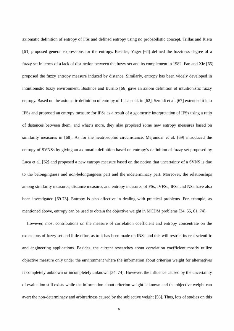
axiomatic definition of entropy of FSs and defined entropy using no probabilistic concept. Trillas and Riera

[63] proposed general expressions for the entropy. Besides, Yager [64] defined the fuzziness degree of a

fuzzy set in terms of a lack of distinction between the fuzzy set and its complement in 1982. Fan and Xie [65]

proposed the fuzzy entropy measure induced by distance. Similarly, entropy has been widely developed in

intuitionistic fuzzy environment. Bustince and Burillo [66] gave an axiom definition of intuitionistic fuzzy

entropy. Based on the axiomatic definition of entropy of Luca et al. in [62], Szmidt et al. [67] extended it into

IFSs and proposed an entropy measure for IFSs as a result of a geometric interpretation of IFSs using a ratio

of distances between them, and what’s more, they also proposed some new entropy measures based on

similarity measures in [68]. As for the neutrosophic circumstance, Majumdar et al. [69] introduced the

entropy of SVNSs by giving an axiomatic definition based on entropy’s definition of fuzzy set proposed by

Luca et al. [62] and proposed a new entropy measure based on the notion that uncertainty of a SVNS is due

to the belongingness and non-belongingness part and the indeterminacy part. Moreover, the relationships

among similarity measures, distance measures and entropy measures of FSs, IVFSs, IFSs and NSs have also

been investigated [69-73]. Entropy is also effective in dealing with practical problems. For example, as

mentioned above, entropy can be used to obtain the objective weight in MCDM problems [34, 55, 61, 74].

However, most contributions on the measure of correlation coefficient and entropy concentrate on the

extensions of fuzzy set and little effort as to it has been made on INSs and this will restrict its real scientific

and engineering applications. Besides, the current researches about correlation coefficient mostly utilize

objective measure only under the environment where the information about criterion weight for alternatives

is completely unknown or incompletely unknown [34, 74]. However, the influence caused by the uncertainty

of evaluation still exists while the information about criterion weight is known and the objective weight can

avert the non-determinacy and arbitrariness caused by the subjective weight [58]. Thus, lots of studies on this

7

issue are needed to be done. Therefore, the correlation coefficient measure, the weighted correlation

coefficient measure and the entropy measure for INSs are extended in this paper and an objective weight

measure based on entropy for INSs is also proposed. Besides, the notion that the weighted correlation

coefficient measure should take use of the integrated weight is put forward. Furthermore, a MCDM

procedure is established based on the weighted correlation coefficient measure which considers both the

subjective weight and the objective weight, and an illustrative example is given to demonstrate the

application of the proposed measures.

The rest of this paper is organized as follows. Section 2 briefly introduces IVIFSs, NSs, SVNSs and INSs

as well as some operations for INSs such as intersection, union. And the correlation coefficient measure, the

weighted correlation coefficient measure, entropy measure, and their properties for INSs are developed in

Section 3. In addition, an objective weight measure making use of entropy for INSs is explored. In Section 4,

decision making procedure based on the weighted correlation coefficient measures using the integrated

weight for MCDM problems are given. In Section 5, an illustrative example is presented to illustrate the

proposed methods and the comparative analysis and discussion are given. Finally, Section 6 concludes the

paper.

2. Preliminaries

In this section, some basic concepts and definitions related to INSs are introduced, which will be used in

the rest of the paper.

Definition 1 [7]. Let X be a space of points (objects), with a generic element in X denoted by x . An IFS

A in X is characterized by a membership function ( )A xµ , and a non-membership function ( )A xν . For

each point x in X , we have ( )A xµ , [ ]( ) 0,1A xν ⊆ , x X∈ . Thus, the IFS A can be denoted by

8

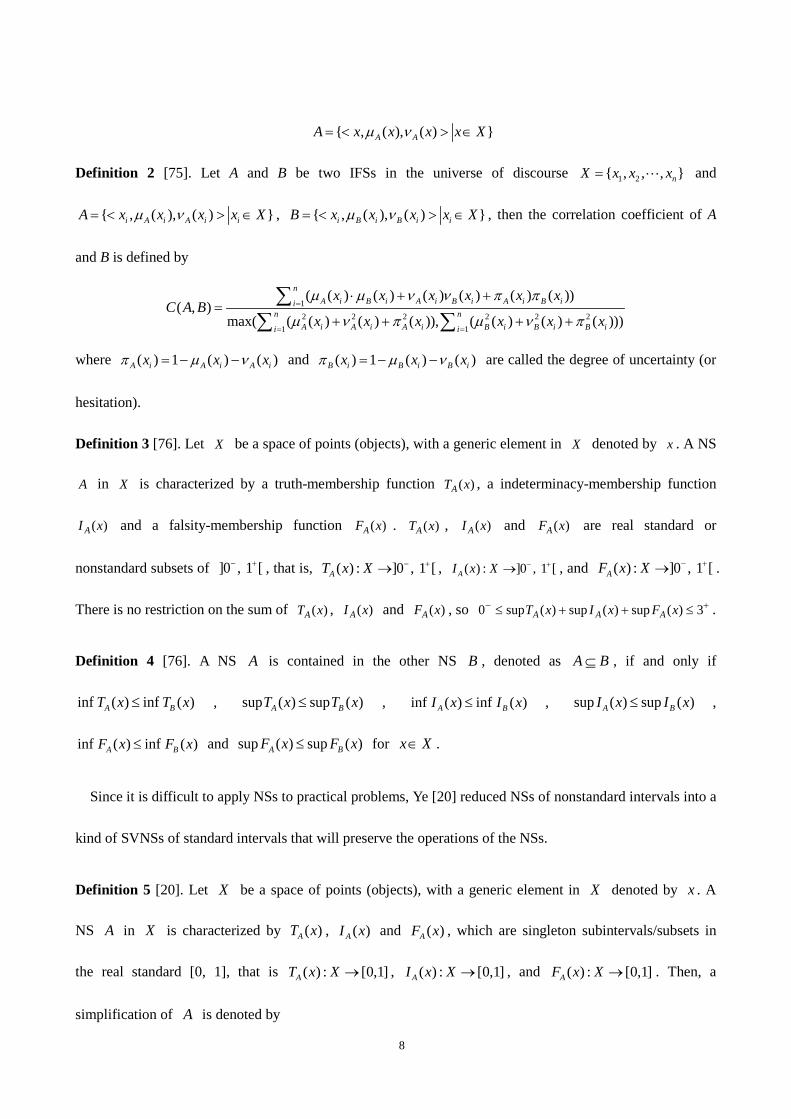
{ , ( ), ( ) }A AA x x x x Xµ ν= < > ∈

Definition 2 [75]. Let A and B be two IFSs in the universe of discourse 1 2{ , , , }nX x x x= and

{ , ( ), ( ) }i A i A i iA x x x x Xµ ν= < > ∈ , { , ( ), ( ) }i B i B i iB x x x x Xµ ν= < > ∈ , then the correlation coefficient of A

and B is defined by

12 2 2 2 2 2

1 1

( ( ) ( ) ( ) ( ) ( ) ( ))( , )

max( ( ( ) ( ) ( )), ( ( ) ( ) ( )))

nA i B i A i B i A i B ii

n nA i A i A i B i B i B ii i

x x x x x xC A B

x x x x x x

µ µ ν ν π π

µ ν π µ ν π=

= =

⋅ + +=

+ + + +

∑∑ ∑

where ( ) 1 ( ) ( )A i A i A ix x xπ µ ν= − − and ( ) 1 ( ) ( )B i B i B ix x xπ µ ν= − − are called the degree of uncertainty (or

hesitation).

Definition 3 [76]. Let X be a space of points (objects), with a generic element in X denoted by x . A NS

A in X is characterized by a truth-membership function )(xTA , a indeterminacy-membership function

)(xI A and a falsity-membership function )(xFA . )(xTA , )(xI A and )(xFA are real standard or

nonstandard subsets of ]0 , 1 [− + , that is, ( ) : ]0 , 1 [AT x X − +→ , ( ) : ]0 , 1 [AI x X − +→ , and ( ) : ]0 , 1 [AF x X − +→ .

There is no restriction on the sum of )(xTA , )(xI A and )(xFA , so +− ≤++≤ 3)(sup)(sup)(sup0 xFxIxT AAA .

Definition 4 [76]. A NS A is contained in the other NS B , denoted as A B⊆ , if and only if

inf ( ) inf ( )A BT x T x≤ , sup ( ) sup ( )A BT x T x≤ , inf ( ) inf ( )A BI x I x≤ , sup ( ) sup ( )A BI x I x≤ ,

inf ( ) inf ( )A BF x F x≤ and sup ( ) sup ( )A BF x F x≤ for x X∈ .

Since it is difficult to apply NSs to practical problems, Ye [20] reduced NSs of nonstandard intervals into a

kind of SVNSs of standard intervals that will preserve the operations of the NSs.

Definition 5 [20]. Let X be a space of points (objects), with a generic element in X denoted by x . A

NS A in X is characterized by ( )AT x , ( )AI x and ( )AF x , which are singleton subintervals/subsets in

the real standard [0, 1], that is ( ) : [0,1]AT x X → , ( ) : [0,1]AI x X → , and ( ) : [0,1]AF x X → . Then, a

simplification of A is denoted by

9

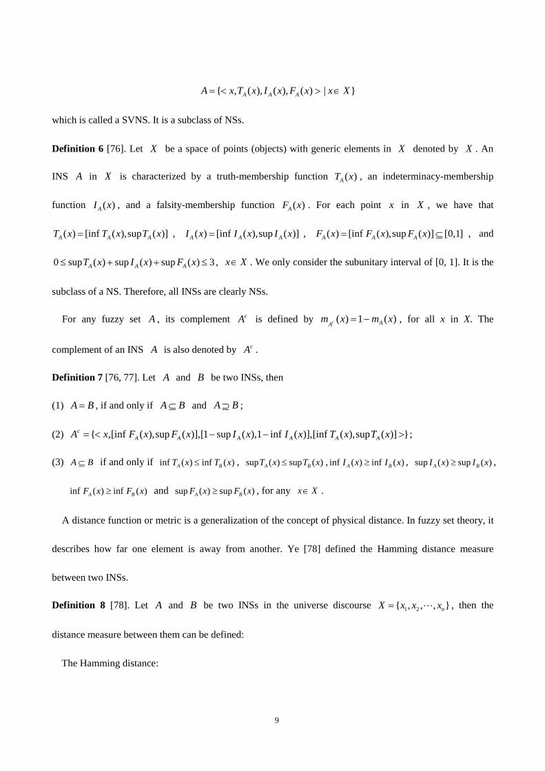
{ , ( ), ( ), ( ) | }A A AA x T x I x F x x X= < > ∈

which is called a SVNS. It is a subclass of NSs.

Definition 6 [76]. Let X be a space of points (objects) with generic elements in X denoted by X . An

INS A in X is characterized by a truth-membership function ( )AT x , an indeterminacy-membership

function ( )AI x , and a falsity-membership function ( )AF x . For each point x in X , we have that

( ) [inf ( ),sup ( )]A A AT x T x T x= , ( ) [inf ( ),sup ( )]A A AI x I x I x= , ( ) [inf ( ),sup ( )] [0,1]A A AF x F x F x= ⊆ , and

0 sup ( ) sup ( ) sup ( ) 3A A AT x I x F x≤ + + ≤ , x X∈ . We only consider the subunitary interval of [0, 1]. It is the

subclass of a NS. Therefore, all INSs are clearly NSs.

For any fuzzy set A , its complement cA is defined by ( ) 1 ( )c AAm x m x= − , for all x in X. The

complement of an INS A is also denoted by cA .

Definition 7 [76, 77]. Let A and B be two INSs, then

(1) A B= , if and only if A B⊆ and A B⊇ ;

(2) { ,[inf ( ),sup ( )],[1 sup ( ),1 inf ( )],[inf ( ),sup ( )] }cA A A A A AA x F x F x I x I x T x T x= < − − > ;

(3) A B⊆ if and only if inf ( ) inf ( )A BT x T x≤ , sup ( ) sup ( )A BT x T x≤ , inf ( ) inf ( )A BI x I x≥ , sup ( ) sup ( )A BI x I x≥ ,

inf ( ) inf ( )A BF x F x≥ and sup ( ) sup ( )A BF x F x≥ , for any x X∈ .

A distance function or metric is a generalization of the concept of physical distance. In fuzzy set theory, it

describes how far one element is away from another. Ye [78] defined the Hamming distance measure

between two INSs.

Definition 8 [78]. Let A and B be two INSs in the universe discourse 1 2{ , , , }nX x x x= , then the

distance measure between them can be defined:

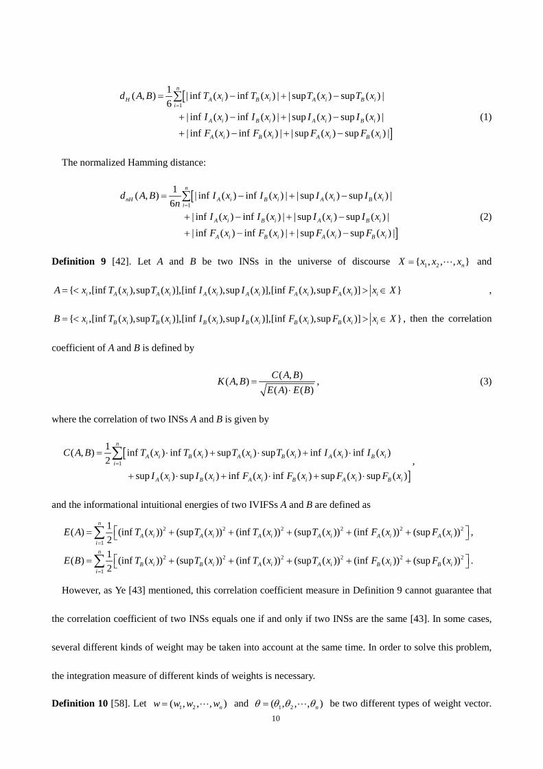
The Hamming distance:

10

[

]

1

1( , ) | inf ( ) inf ( ) | | sup ( ) sup ( ) |6

| inf ( ) inf ( ) | | sup ( ) sup ( ) | | inf ( ) inf ( ) | | sup ( ) sup ( ) |

n

H A i B i A i B ii

A i B i A i B i

A i B i A i B i

d A B T x T x T x T x

I x I x I x I xF x F x F x F x

== − + −

+ − + −

+ − + −

∑

(1)

The normalized Hamming distance:

[

]

1

1( , ) | inf ( ) inf ( ) | | sup ( ) sup ( ) |6

| inf ( ) inf ( ) | | sup ( ) sup ( ) | | inf ( ) inf ( ) | | sup ( ) sup ( ) |

n

nH A i B i A i B ii

A i B i A i B i

A i B i A i B i

d A B I x I x I x I xn

I x I x I x I xF x F x F x F x

== − + −

+ − + −

+ − + −

∑

(2)

Definition 9 [42]. Let A and B be two INSs in the universe of discourse 1 2{ , , , }nX x x x= and

{ ,[inf ( ),sup ( )],[inf ( ),sup ( )],[inf ( ),sup ( )] }i A i A i A i A i A i A i iA x T x T x I x I x F x F x x X= < > ∈ ,

{ ,[inf ( ),sup ( )],[inf ( ),sup ( )],[inf ( ),sup ( )] }i B i B i B i B i B i B i iB x T x T x I x I x F x F x x X= < > ∈ , then the correlation

coefficient of A and B is defined by

( , )( , )( ) ( )C A BK A B

E A E B=

⋅, (3)

where the correlation of two INSs A and B is given by

[

]1

1( , ) inf ( ) inf ( ) sup ( ) sup ( ) inf ( ) inf ( )2

sup ( ) sup ( ) inf ( ) inf ( ) sup ( ) sup ( )

n

A i B i A i B i A i B ii

A i B i A i B i A i B i

C A B T x T x T x T x I x I x

I x I x F x F x F x F x=

= ⋅ + ⋅ + ⋅

+ ⋅ + ⋅ + ⋅

∑ ,

and the informational intuitional energies of two IVIFSs A and B are defined as

2 2 2 2 2 2

1

1( ) (inf ( )) (sup ( )) (inf ( )) (sup ( )) (inf ( )) (sup ( ))2

n

A i A i A i A i A i A ii

E A T x T x T x T x F x F x=

= + + + + + ∑ ,

2 2 2 2 2 2

1

1( ) (inf ( )) (sup ( )) (inf ( )) (sup ( )) (inf ( )) (sup ( ))2

n

B i B i A i A i B i B ii

E B T x T x T x T x F x F x=

= + + + + + ∑ .

However, as Ye [43] mentioned, this correlation coefficient measure in Definition 9 cannot guarantee that

the correlation coefficient of two INSs equals one if and only if two INSs are the same [43]. In some cases,

several different kinds of weight may be taken into account at the same time. In order to solve this problem,

the integration measure of different kinds of weights is necessary.

Definition 10 [58]. Let 1 2( , , , )nw w w w= and 1 2( , , , )nθ θ θ θ= be two different types of weight vector.

11

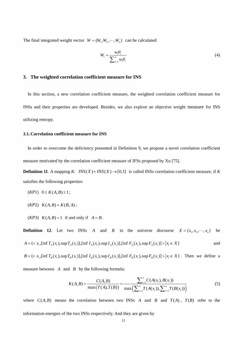
The final integrated weight vector 1 2( , , , )nW W W W= can be calculated:

1

i ii n

i ii

wWwθθ

=

=∑

(4)

3. The weighted correlation coefficient measure for INS

In this section, a new correlation coefficient measure, the weighted correlation coefficient measure for

INSs and their properties are developed. Besides, we also explore an objective weight measure for INS

utilizing entropy.

3.1. Correlation coefficient measure for INS

In order to overcome the deficiency presented in Definition 9, we propose a novel correlation coefficient

measure motivated by the correlation coefficient measure of IFSs proposed by Xu [75].

Definition 11. A mapping K: ( ) ( ) [0,1]INS X INS X× → is called INSs correlation coefficient measure, if K

satisfies the following properties:

(KP1) 0 ( , ) 1K A B≤ ≤ ;

(KP2) ( , ) ( , )K A B K B A= ;

(KP3) ( , ) 1K A B = if and only if A B= .

Definition 12. Let two INSs A and B in the universe discourse 1 2{ , , , }nX x x x= be

{ ,[inf ( ),sup ( )],[inf ( ),sup ( )],[inf ( ),sup ( )] }i A i A i A i A i A i A i iA x T x T x I x I x F x F x x X= < > ∈ and

{ ,[inf ( ),sup ( )],[inf ( ),sup ( )],[inf ( ),sup ( )] }i B i B i B i B i B i B i iB x T x T x I x I x F x F x x X= < > ∈ . Then we define a

measure between A and B by the following formula:

( ) ( )1

1 1

( ( ), ( ))( , )( , )max ( ), ( ) max ( ( )), ( ( ))

ni ii

n ni ii i

C A x B xC A BK A BT A T B T A x T B x

=

= =

= = ∑∑ ∑

(5)

where ( , )C A B means the correlation between two INSs A and B and ( )T A , ( )T B refer to the

information energies of the two INSs respectively. And they are given by

12

1( ( ), ( )) [inf ( ) inf ( ) sup ( ) sup ( ) inf ( ) inf ( )2

sup ( ) sup ( ) inf ( ) inf ( ) sup ( ) sup ( )]

i i A i B i A i B i A i B i

A i B i A i B i A i B i

C A x B x T x T x T x T x I x I x

I x I x F x F x F x F x

= ⋅ + ⋅ + ⋅

+ ⋅ + ⋅ + ⋅, (6)

2 2 2 2 2 2(inf ( )) +(sup ( )) (inf ( )) +(sup ( )) (inf ( )) +(sup ( ))( ( ))2

A i A i A i A i A i A ii

T x T x I x I x F x F xT A x + += , (7)

2 2 2 2 2 2(inf ( )) +(sup ( )) (inf ( )) +(sup ( )) (inf ( )) +(sup ( ))( ( ))2

B i B i B i B i B i B ii

T x T x I x I x F x F xT B x + += . (8)

Theorem 1. The proposed measure ( , )K A B satisfies all the axioms given in Definition 11.

Proof.

(KP1) According to Definition 6, [inf ( ),sup ( )]A i A iT x T x , [inf ( ),sup ( )]A i A iI x I x , [inf ( ),sup ( )]A i A iF x F x ,

[inf ( ),sup ( )]B i B iT x T x , [inf ( ),sup ( )]B i B iI x I x and [inf ( ),sup ( )] [0,1]B i B iF x F x ⊆ exist for any

{1,2, , }i n∈ . Thus, it holds that ( , ) 0C A B ≥ , ( ) 0T A ≥ and ( ) 0T B ≥ . Therefore,

( )( , )( , ) 0

max ( ), ( )C A BK A BT A T B

= ≥ . According to the Cauchy–Schwarz inequality:

( ) ( ) ( )2 2 2 2 2 2 21 1 2 2 1 2 1 2n n n na b a b a b a a a b b b+ + + ≤ + + + ⋅ + + + where ,i ia b R∈ , 1,2, ,i n= ,

( )( , )( , ) 1

max ( ), ( )C A BK A BT A T B

= ≤ . Therefore, 0 ( , ) 1K A B≤ ≤ holds.

(KP2) According to Equation (6), we know that ( , ) ( , )C A B C B A= , and it’s obviously

( ) ( )( , ) ( , )( , ) ( , )

max ( ), ( ) max ( ), ( )C A B C A BK A B K B AT A T B T B T A

= = = .

(KP3) If A B= , we have that inf ( ) inf ( )A i B iT x T x= , sup ( ) sup ( )A i B iT x T x= , inf ( ) inf ( )A i B iI x I x= ,

sup ( ) sup ( )A i B iI x I x= , inf ( ) inf ( )A i B iF x F x= and sup ( ) sup ( )A i B iF x F x= . So,

2 2 2 2 2 21

1( , ) [(inf ( )) +(sup ( )) (inf ( )) +(sup ( )) (inf ( )) +(sup ( )) ]2

nA A i A i A i A i A ii

C A B T x T x I x I x F x F x=

= + +∑ and

2 2 2 2 2 21

1( ) ( ) [(inf ( )) +(sup ( )) (inf ( )) +(sup ( )) (inf ( )) +(sup ( )) ]2

nA i A i A i A i A i A ii

T A T B T x T x I x I x F x F x=

= = + +∑ ,

i.e. ( , ) ( ) ( )C A B T A T B= = . Thus, it is clear that ( )

( , )( , ) 1max ( ), ( )

C A BK A BT A T B

= = .

If ( )

( , )( , ) 1max ( ), ( )

C A BK A BT A T B

= = , then ( , ) max( ( ), ( ))C A B T A T B= . According to the Cauchy–Schwarz

13

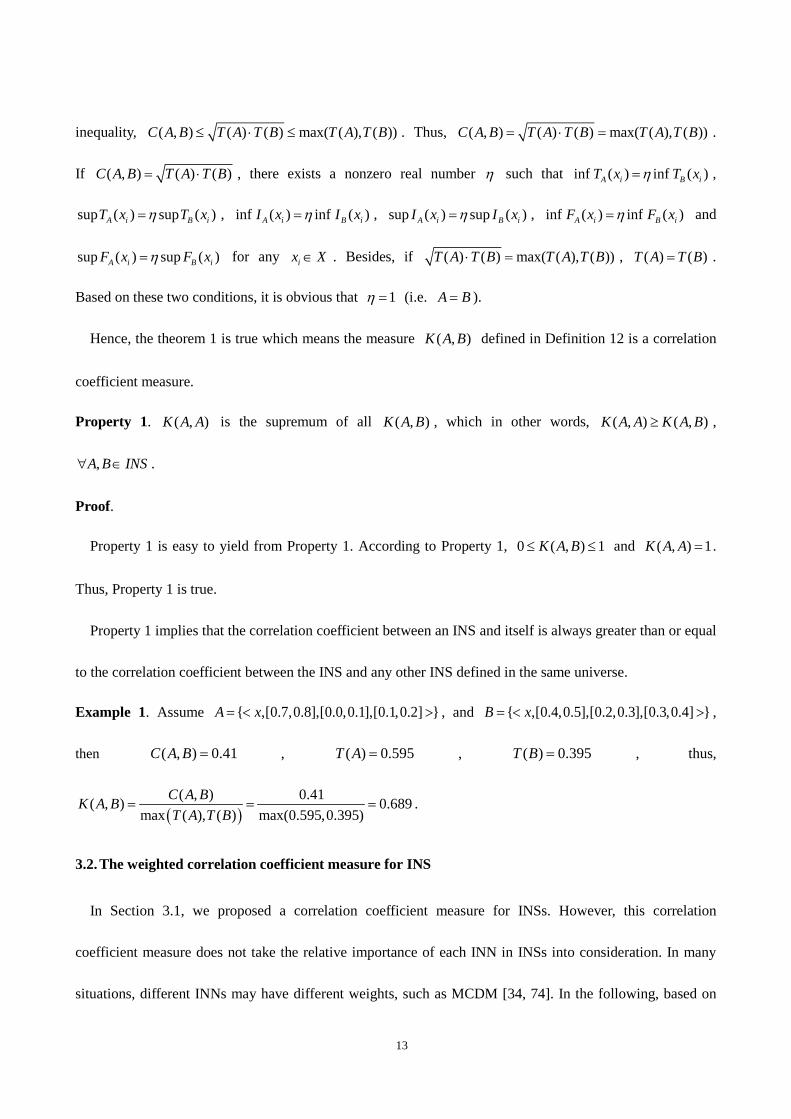
inequality, ( , ) ( ) ( ) max( ( ), ( ))C A B T A T B T A T B≤ ⋅ ≤ . Thus, ( , ) ( ) ( ) max( ( ), ( ))C A B T A T B T A T B= ⋅ = .

If ( , ) ( ) ( )C A B T A T B= ⋅ , there exists a nonzero real number η such that inf ( ) inf ( )A i B iT x T xη= ,

sup ( ) sup ( )A i B iT x T xη= , inf ( ) inf ( )A i B iI x I xη= , sup ( ) sup ( )A i B iI x I xη= , inf ( ) inf ( )A i B iF x F xη= and

sup ( ) sup ( )A i B iF x F xη= for any ix X∈ . Besides, if ( ) ( ) max( ( ), ( ))T A T B T A T B⋅ = , ( ) ( )T A T B= .

Based on these two conditions, it is obvious that 1η = (i.e. A B= ).

Hence, the theorem 1 is true which means the measure ( , )K A B defined in Definition 12 is a correlation

coefficient measure.

Property 1. ( , )K A A is the supremum of all ( , )K A B , which in other words, ( , ) ( , )K A A K A B≥ ,

,A B INS∀ ∈ .

Proof.

Property 1 is easy to yield from Property 1. According to Property 1, 0 ( , ) 1K A B≤ ≤ and ( , ) 1K A A = .

Thus, Property 1 is true.

Property 1 implies that the correlation coefficient between an INS and itself is always greater than or equal

to the correlation coefficient between the INS and any other INS defined in the same universe.

Example 1. Assume { ,[0.7,0.8],[0.0,0.1],[0.1,0.2] }A x= < > , and { ,[0.4,0.5],[0.2,0.3],[0.3,0.4] }B x= < > ,

then ( , ) 0.41C A B = , ( ) 0.595T A = , ( ) 0.395T B = , thus,

( )( , ) 0.41( , ) 0.689

max ( ), ( ) max(0.595,0.395)C A BK A BT A T B

= = = .

3.2. The weighted correlation coefficient measure for INS

In Section 3.1, we proposed a correlation coefficient measure for INSs. However, this correlation

coefficient measure does not take the relative importance of each INN in INSs into consideration. In many

situations, different INNs may have different weights, such as MCDM [34, 74]. In the following, based on

14

the correlation coefficient measure between INSs defined in Definition 12, the weighted correlation

coefficient between INSs will be introduced.

Definition 13. Let { ,[inf ( ),sup ( )],[inf ( ),sup ( )],[inf ( ),sup ( )] }i A i A i A i A i A i A i iA x T x T x I x I x F x F x x X= < > ∈

and { ,[inf ( ),sup ( )],[inf ( ),sup ( )],[inf ( ),sup ( )] }i B i B i B i B i B i B i iB x T x T x I x I x F x F x x X= < > ∈ be two INSs in

the universe discourse 1 2{ , , , }nX x x x= . Let 1 2{ , , , }nw w w w= be the weight vector of the elements

ix ( 1,2, , )i n= . Then we can define a measure between A and B by the following formula:

( )1

1 1

( ( ), ( ))( , )

max ( ( )), ( ( ))

ni i ii

n ni i i ii i

w C A x B xK A B

wT A x wT B x=

= =

= ∑∑ ∑

(9)

where ( ( ), ( ))i iC A x B x , ( ( ))iT A x and ( ( ))iT B x satisfy Equations (6)-(8).

Theorem 2. The proposed measure ( , )K A B in Definition 13 satisfies all the axioms given in Definition 11.

Proof.

(P1) According to Property 1, ( ( ), ( )) 0i iC A x B x ≥ , ( ( )) 0iT A x ≥ and ( ( )) 0iT B x ≥ ( 1,2, , )i n= .

Besides, 0iw ≥ , thus, ( )

1

1 1

( ( ), ( ))( , ) 0

max ( ( )), ( ( ))

ni i ii

n ni i i ii i

w C A x B xK A B

wT A x wT B x=

= =

= >∑∑ ∑

. According to the

Cauchy–Schwarz inequality,

11 1 1 1

( ( ), ( )) ( ( )) ( ( )) max ( ( )), ( ( ))n n n n

ni i i i i i i i i i ii

i i i iw C A x B x wT A x wT B x wT A x wT B x

== = = =

≤ ≤

∑ ∑ ∑ ∑ ∑ . Therefore,

( , ) 1K A B ≤ .

(P2) According to Property 1, we know that ( ( ), ( )) ( ( ), ( ))i i i iC A x B x C B x A x= exists for any

{ ,2, , }i i n∈ . Therefore, it’s obvious that 1 1

( ( ), ( )) ( ( ), ( ))n ni i i i i ii i

w C A x B x w C B x A x= =

=∑ ∑ . Thus,

( ) ( )1 1

1 1 1 1

( ( ), ( )) ( ( ), ( ))( , ) ( , )

max ( ( )), ( ( )) max ( ( )), ( ( ))

n ni i i i i ii i

n n n ni i i i i i i ii i i i

w C A x B x w C B x A xK A B K B A

wT A x wT B x wT B x wT A x= =

= = = =

= = =∑ ∑∑ ∑ ∑ ∑

.

15

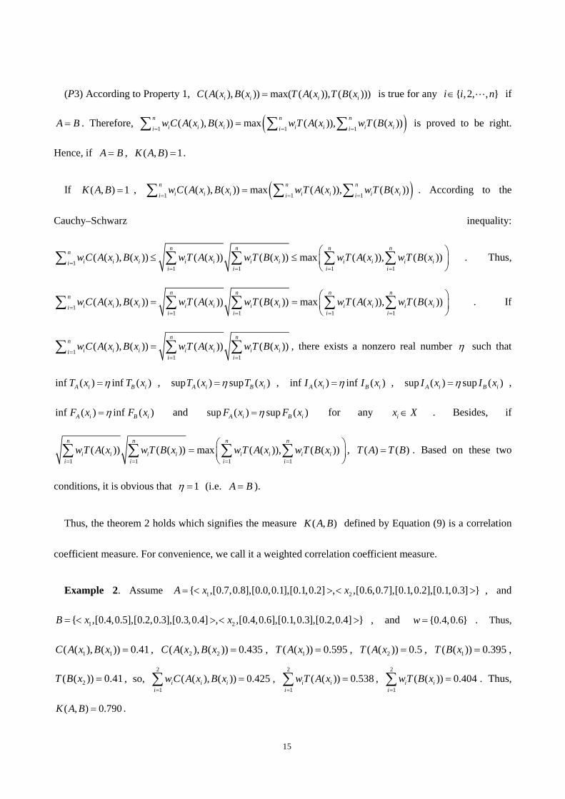
(P3) According to Property 1, ( ( ), ( )) max( ( ( )), ( ( )))i i i iC A x B x T A x T B x= is true for any { ,2, , }i i n∈ if

A B= . Therefore, ( )1 1 1( ( ), ( )) max ( ( )), ( ( ))n n n

i i i i i i ii i iw C A x B x wT A x wT B x

= = ==∑ ∑ ∑ is proved to be right.

Hence, if A B= , ( , ) 1K A B = .

If ( , ) 1K A B = , ( )1 1 1( ( ), ( )) max ( ( )), ( ( ))n n n

i i i i i i ii i iw C A x B x wT A x wT B x

= = ==∑ ∑ ∑ . According to the

Cauchy–Schwarz inequality:

11 1 1 1

( ( ), ( )) ( ( )) ( ( )) max ( ( )), ( ( ))n n n n

ni i i i i i i i i i ii

i i i iw C A x B x wT A x wT B x wT A x wT B x

== = = =

≤ ≤

∑ ∑ ∑ ∑ ∑ . Thus,

11 1 1 1

( ( ), ( )) ( ( )) ( ( )) max ( ( )), ( ( ))n n n n

ni i i i i i i i i i ii

i i i iw C A x B x wT A x wT B x wT A x wT B x

== = = =

= =

∑ ∑ ∑ ∑ ∑ . If

11 1

( ( ), ( )) ( ( )) ( ( ))n n

ni i i i i i ii

i iw C A x B x wT A x wT B x

== =

=∑ ∑ ∑ , there exists a nonzero real number η such that

inf ( ) inf ( )A i B iT x T xη= , sup ( ) sup ( )A i B iT x T xη= , inf ( ) inf ( )A i B iI x I xη= , sup ( ) sup ( )A i B iI x I xη= ,

inf ( ) inf ( )A i B iF x F xη= and sup ( ) sup ( )A i B iF x F xη= for any ix X∈ . Besides, if

1 1 1 1( ( )) ( ( )) max ( ( )), ( ( ))

n n n n

i i i i i i i ii i i i

wT A x wT B x wT A x wT B x= = = =

=

∑ ∑ ∑ ∑ , ( ) ( )T A T B= . Based on these two

conditions, it is obvious that 1η = (i.e. A B= ).

Thus, the theorem 2 holds which signifies the measure ( , )K A B defined by Equation (9) is a correlation

coefficient measure. For convenience, we call it a weighted correlation coefficient measure.

Example 2. Assume 1 2{ ,[0.7,0.8],[0.0,0.1],[0.1,0.2] , ,[0.6,0.7],[0.1,0.2],[0.1,0.3] }A x x= < > < > , and

1 2{ ,[0.4,0.5],[0.2,0.3],[0.3,0.4] , ,[0.4,0.6],[0.1,0.3],[0.2,0.4] }B x x= < > < > , and {0.4,0.6}w = . Thus,

1 1( ( ), ( )) 0.41C A x B x = , 2 2( ( ), ( )) 0.435C A x B x = , 1( ( )) 0.595T A x = , 2( ( )) 0.5T A x = , 1( ( )) 0.395T B x = ,

2( ( )) 0.41T B x = , so, 2

1( ( ), ( )) 0.425i i i

iw C A x B x

=

=∑ , 2

1( ( )) 0.538i i

iwT A x

=

=∑ , 2

1( ( )) 0.404i i

iwT B x

=

=∑ . Thus,

( , ) 0.790K A B = .

16

As noted in Section 1, the integrated weight can benefit from not only decision makers’ expertise but also

the relative importance of evaluation information. In order to assess the relative importance or weights

accurately and comprehensively, it’s better to utilize the integrated weight rather than only the subjective

weight or objective weight to obtain the weighted correlation coefficient here.

The subjective weight and the objective weight should be calculated in order to compute the integrated

weight. The subjective weight mirroring the individual preference can be evaluated by the decision maker

while the objective weight reflecting the relative importance contained in the decision matrix should be

calculated by mathematical methods. Certainly, many kinds of objective weight measures have been

proposed and every measure has its own advantages [79, 80]. Because of the fact that the more equivocal the

information is, the less important it will be [81], we utilize the entropy weight measure to obtain the

objective weight.

3.3 The entropy weight measure for INS

In this section, we propose the entropy measure and an objective weight measure based on entropy for

INS.

Entropy is an important concept named after Claude Shannon who introduced the concept first. In

information theory, entropy is a measure for calculating the uncertainty associated with a random variable. It

characterizes the uncertainty about the source of information. Thus entropy is as a measure of uncertainty.

Based on the axiomatic definition of entropy measure for SVNSs in [69], the entropy for INSs can be defined

as follows.

Definition 14. A real function : ( ) [0,1]E INS X → is called entropy on INS(X), if E satisfies the following

properties,

(EP1) ( ) 0E A = (minimum) if A is a crisp set ( ( ))A P X∀ ∈ ;

17

(EP2) ( ) 1E A = (maximum) if ( ) ( ) ( )A A AT x I x F x= = (i.e. inf ( ) inf ( ) inf ( )A A AT x I x F x= = and

sup ( ) sup ( ) sup ( )A A AT x I x F x= = ) for any x X∈ ;

(EP3) ( ) ( )E A E B≤ if A is less fuzzy than B or B is more uncertain than A , i.e. (1)

inf ( ) inf ( ) inf ( ) inf ( )A A B BT x F x I x F x− ≤ − and sup ( ) sup ( ) sup ( ) sup ( )A A B BT x F x I x F x− ≤ − for

inf ( ) inf ( )A AT x F x≥ and sup ( ) sup ( )A AT x F x≤ or inf ( ) inf ( ) inf ( ) inf ( )A A B BT x F x I x F x− ≥ − and

sup ( ) sup ( ) sup ( ) sup ( )A A B BT x F x I x F x− ≥ − for inf ( ) inf ( )A AT x F x≤ and sup ( ) sup ( )A AT x F x≤ and

sup ( ) sup ( )A BT x T x≥ ; and (2) inf ( ) inf ( )A BI x I x≤ and sup ( ) sup ( )A BI x I x≤ for

inf ( ) sup ( ) 1B BI x I x+ ≤ or inf ( ) inf ( )A BI x I x≥ and sup ( ) sup ( )A BI x I x≥ for inf ( ) sup ( ) 1B BI x I x+ ≥ ;

(EP4) ( ) ( )cE A E A= .

Great quantities of researches have demonstrated the connection among the distance measure, the

similarity measure and the entropy measure of fuzzy sets [69-73]. According to these studies, we propose the

entropy measure of INSs based on the distance measure defined in Definition 8.

Definition 15. Let A be an INS in the universe discourse 1 2{ , , , }nX x x x= , and assume that

( ) : ( ) [0,1]E A N X → . ( )E A is a measure such that

( ) 1 ( , )cE A d A A= − . (10)

where ( , )cd A A refers to the distance measure between INS A and its complementary set cA utilizing

Equation (2).

Theorem 3. The proposed measure ( )E A satisfies all the axioms given in Definition 14.

Proof. Let { ,[inf ( ),sup ( )],[inf ( ),sup ( )],[inf ( ),sup ( )] }i A i A i A i A i A i A i iA x T x T x I x I x F x F x x X= < > ∈ and

{ ,[inf ( ),sup ( )],[inf ( ),sup ( )],[inf ( ),sup ( )] }i B i B i B i B i B i B i iB x T x T x I x I x F x F x x X= < > ∈ be two INSs.

(EP1) If an INS A is a crisp set, i.e. inf ( ) sup ( ) 1A i A iT x T x= = , inf ( ) sup ( ) 0A i A iI x I x= = ,

inf ( ) sup ( ) 0A i A iF x F x= = or inf ( ) sup ( ) 0A i A iT x T x= = , inf ( ) sup ( ) 1A i A iI x I x= = ,

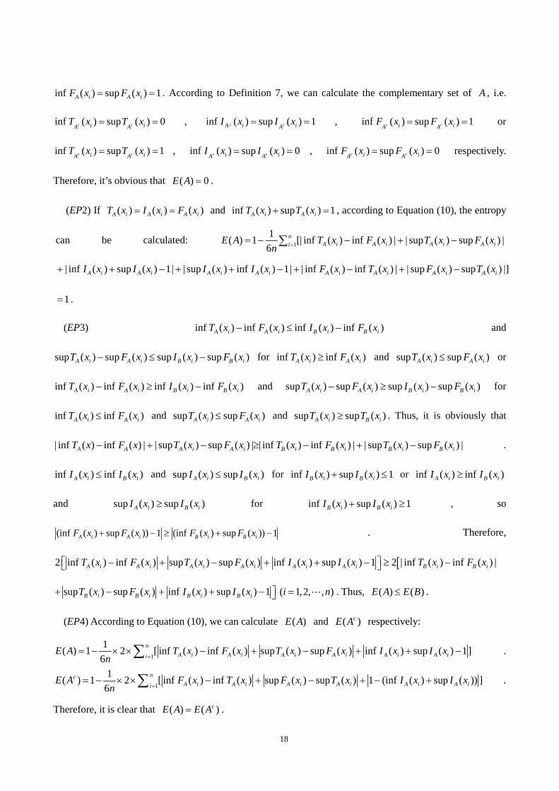
18

inf ( ) sup ( ) 1A i A iF x F x= = . According to Definition 7, we can calculate the complementary set of A , i.e.

inf ( ) sup ( ) 0c ci iA AT x T x= = , inf ( ) sup ( ) 1c cA i iA

I x I x= = , inf ( ) sup ( ) 1c ci iA AF x F x= = or

inf ( ) sup ( ) 1c ci iA AT x T x= = , inf ( ) sup ( ) 0c ci iA A

I x I x= = , inf ( ) sup ( ) 0c ci iA AF x F x= = respectively.

Therefore, it’s obvious that ( ) 0E A = .

(EP2) If ( ) ( ) ( )A i A i A iT x I x F x= = and inf ( ) sup ( ) 1A i A iT x T x+ = , according to Equation (10), the entropy

can be calculated: 11( ) 1 [| inf ( ) inf ( ) | | sup ( ) sup ( ) |

6n

A i A i A i A iiE A T x F x T x F xn == − − + −∑

| inf ( ) sup ( ) 1| | sup ( ) inf ( ) 1| | inf ( ) inf ( ) | | sup ( ) sup ( ) |]A i A i A i A i A i A i A i A iI x I x I x I x F x T x F x T x+ + − + + − + − + −

1= .

(EP3) inf ( ) inf ( ) inf ( ) inf ( )A i A i B i B iT x F x I x F x− ≤ − and

sup ( ) sup ( ) sup ( ) sup ( )A i A i B i B iT x F x I x F x− ≤ − for inf ( ) inf ( )A i A iT x F x≥ and sup ( ) sup ( )A i A iT x F x≤ or

inf ( ) inf ( ) inf ( ) inf ( )A i A i B i B iT x F x I x F x− ≥ − and sup ( ) sup ( ) sup ( ) sup ( )A i A i B i B iT x F x I x F x− ≥ − for

inf ( ) inf ( )A i A iT x F x≤ and sup ( ) sup ( )A i A iT x F x≤ and sup ( ) sup ( )A i B iT x T x≥ . Thus, it is obviously that

| inf ( ) inf ( ) | | sup ( ) sup ( ) | | inf ( ) inf ( ) | | sup ( ) sup ( ) |A A A i A i B i B i B i B iT x F x T x F x T x F x T x F x− + − ≥ − + − .

inf ( ) inf ( )A i B iI x I x≤ and sup ( ) sup ( )A i B iI x I x≤ for inf ( ) sup ( ) 1B i B iI x I x+ ≤ or inf ( ) inf ( )A i B iI x I x≥

and sup ( ) sup ( )A i B iI x I x≥ for inf ( ) sup ( ) 1B i B iI x I x+ ≥ , so

(inf ( ) sup ( )) 1 (inf ( ) sup ( )) 1A i A i B i B iF x F x F x F x+ − ≥ + − . Therefore,

[2 inf ( ) inf ( ) sup ( ) sup ( ) inf ( ) sup ( ) 1 2 | inf ( ) inf ( ) |A i A i A i A i A i A i B i B iT x F x T x F x I x I x T x F x − + − + + − ≥ −

sup ( ) sup ( ) inf ( ) sup ( ) 1B i B i B i B iT x F x I x I x + − + + − ( 1,2, , )i n= . Thus, ( ) ( )E A E B≤ .

(EP4) According to Equation (10), we can calculate ( )E A and ( )cE A respectively:

1

1( ) 1 2 [ inf ( ) inf ( ) sup ( ) sup ( ) inf ( ) sup ( ) 1]6

nA i A i A i A i A i A ii

E A T x F x T x F x I x I xn =

= − × × − + − + + −∑ .

1

1( ) 1 2 [ inf ( ) inf ( ) sup ( ) sup ( ) 1 (inf ( ) sup ( )) ]6

ncA i A i A i A i A i A ii

E A F x T x F x T x I x I xn =

= − × × − + − + − +∑ .

Therefore, it is clear that ( ) ( )cE A E A= .

19

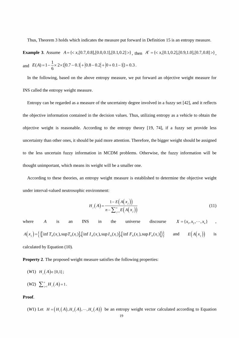
Thus, Theorem 3 holds which indicates the measure put forward in Definition 15 is an entropy measure.

Example 3. Assume { ,[0.7,0.8],[0.0,0.1],[0.1,0.2] }A x= < > , then { ,[0.1,0.2],[0.9,1.0],[0.7,0.8] }cA x= < > ,

and 1( ) 1 2 [ 0.7 0.1 0.8 0.2 0 0.1 1] 0.36

E A = − × × − + − + + − = .

In the following, based on the above entropy measure, we put forward an objective weight measure for

INS called the entropy weight measure.

Entropy can be regarded as a measure of the uncertainty degree involved in a fuzzy set [42], and it reflects

the objective information contained in the decision values. Thus, utilizing entropy as a vehicle to obtain the

objective weight is reasonable. According to the entropy theory [19, 74], if a fuzzy set provide less

uncertainty than other ones, it should be paid more attention. Therefore, the bigger weight should be assigned

to the less uncertain fuzzy information in MCDM problems. Otherwise, the fuzzy information will be

thought unimportant, which means its weight will be a smaller one.

According to these theories, an entropy weight measure is established to determine the objective weight

under interval-valued neutrosophic environment:

( )( )( )( )( )1

1j n

j

j

j

E AH

n E A

xA

x=

−=

−∑ (11)

where A is an INS in the universe discourse 1 2{ , , , }nX x x x= ,

( ) [ ] [ ] [ ]{ }inf ( ),sup ( ) , inf ( ),sup ( ) , inf ( ),sup ( )j A i A i A i A i A i A iA x T x T x I x I x F x F x= and ( )( )jE A x is

calculated by Equation (10).

Property 2. The proposed weight measure satisfies the following properties:

(W1) ( ) [0,1]jH A ∈ ;

(W2) ( )11n

jjH A

==∑ .

Proof.

(W1) Let ( ) ( ) ( )( )1 2, , , nH H H HA A A= be an entropy weight vector calculated according to Equation

20

(11). According to Theorem 3, we know that entropy value of INSs lies between 0 and 1, i.e.

( )( ) [0,1]jE A x ∈ , thus, it’s obvious that ( )( )1 [0,1]jE A x− ∈ and ( )( )1[0,1]n

jjn E A x

=− ∈∑ . Besides,

( )( )( ) ( )( ) ( )( )11,

1 1 0n

nj j jj

i i jE A x n E A x n E A x

== ≠

− + − + = − ≥

∑ ∑ and ( )( )

1,1 0

n

ji i j

n E A x= ≠

− + ≥

∑ hold

which means ( )( ) ( )( )( )11n

j jjn E A x E A x

=− ≥ −∑ is true. Based on these conclusions, we can obtain that

( )( )( )

( )( )1

1[0,1]j n

j

j

j

E AH

n E A

xA

x=

−=

−∈

∑.

(W2) It is clear that ( ) ( )( )( )( )

( )( )( )( )

( )( )( )( )1 1

1

1 1

1 1

1 11n n j

j nj jjj

n nj jj j

n nj jj j

E A x

n E A x

E A x n E A xH A

n E A x n E A x= =

=

= =

= =

−=

−

− −= = =

− −∑ ∑

∑∑ ∑∑ ∑

.

Therefore, Property 2 holds.

Example 4. Assume 1 2{ ,[0.7,0.8],[0.0,0.1],[0.1,0.2] , ,[0.4,0.5],[0.2,0.3],[0.3,0.4] ,A x x= < > < >

3 ,[0.6,0.7],[0.1,0.2],[0.1,0.3] }x< > . According to Equation (10), we can figure out that ( )( )1 0.3E A x = ,

( )( )2 0.767E A x = and ( )( )3 0.467E A x = . And according to Equation (11), ( )1 0.477H A = ,

( )1 0.159H B = and ( )1 0.364H C = .

Example 5. Assume that there are three INSs

1 2{ ,[0.4,0.5],[0.0,0.1],[0.3,0.4] , ,[0.6,0.7],[0.4,0.5],[0.1,0.3] }A x x= < > < > ,

1 2{ ,[0.7,0.8],[0.0,0.1],[0.1,0.2] , ,[0.2,0.4],[0.5,0.6],[0.2,0.4] }B x x= < > < > and

1 2{ ,[1,1],[0,0],[0,0] , ,[1,1],[0,0],[0,0] }C x x= < > < > , and (0.5,0.5)w = is the subjective weight vector.

According to Equation (9), the weighted correlation coefficient based on the subjective weight can be

calculated: ( , ) 0.55K A C = and ( , ) 0.525K B C = . Therefore, ( , ) ( , )K A C K B C> is true which means that

the relative similarity degree between A and C is more than that between B and C . What’s more,

according to Equation (11), the objective weight matrix can be obtained: (0.52,0.48)AH = ,

(0.95,0.05)BH = and according to Equation (4), the integrated weight matrix is 0.52 0.480.95 0.05

W =

.

21

According to Equation (9), the weighted correlation coefficient based on the subjective weight can be

calculated: ( , ) 0.546K A C = and ( , ) 0.728K B C = . Thus, ( , ) ( , )K A C K B C< is true which means that the

relative similarity degree between A and C is less than that between B and C .

The above example shows that the relative similarity degree may be different when using two different

kinds of weight. The cause lies in the fact that the subjective weight reflects only the preference of decision

maker and ignores the objective information included in the decision matrix; by contrast, the integrated

weight can benefit from not only decision makers’ expertise but also the relative importance of evaluation

information.

4. The weighted correlation coefficient application to multi-criteria decision making

problems

In this section, we present a model for MCDM problems applying the weighted correlation coefficient

measures for INSs and taking the integration of objective weight and subjective weight into account.

Assume there are m alternatives 1{ ,A A= 2 ,A , }mA and n criteria 1{ ,C C= 2 ,C , }nC , whose

subjective weight vector provided by the decision maker is 1 2( , , , )nw w w w= , where 0jw ≥

( 1,2, ,j n= ), 1

1n

jj

w=

=∑ . Let ( )ij m nR a ×= be the interval neutrosophic decision matrix, where

, ,ij ij ijij a a aa T I F= ⟨ ⟩ is an evaluation value, denoted by INN, where [inf ,sup ]

ij ij ija a aT T T= indicates the

truth-membership function that the alternative iA satisfies the criterion jC , [inf ,sup ]ij ij ija a aI I I=

indicates the indeterminacy-membership function that the alternative iA satisfies the criterion jC and

[inf ,sup ]ij ij ija a aF F F= indicates the falsity-membership function that the alternative iA satisfies the

criterion jC .

In MCDM environments, the concept of ideal point has been used to help identify the best alternative in

22

the decision set [34]. An ideal alternative can be identified by using a maximum operator to determine the

best value of each criterion among all alternatives [78]. Thus, we defined an ideal INN in the ideal alternative

*A as

* * * * * * *= [a , ],[ , ],[ , ]

[max(a ),max( )],[min(a ),min( )],[min(a ),min( )]

j j j j j j j

ij ij ij ij ij iji i i ii i

b c d e f

b b b

a

=, (12)

where { }1,2, ,i m∈ and 1,2, ,j n= .

Based on Equation (10) and the integrated weight matrix

11 12 1

21 22 2

1 2

n

n

m m mn

W W WW W W

W

W W W

=

where ijW is the

integrated weight of alternative iA under criterion jC , we can denote the weighted correlation coefficient

measure between the alternative iA and the ideal alternative A∗ as

( )( )( )* * * * * *

1*

* 2 * 2 * 2 * 2 * 2 * 21 1

[a (inf ) (sup )+c (inf ) (sup )+ (inf ) (sup )]( , )

max , [(a ) (b ) ( ) ( ) ( ) ( ) ]ij ij ij ij ij ij

nij j a j a j a j a j a j aj

i n nij i j ij j j j j j jj j

W T b T I d I e F f FK A A

W T A x W c d e f=

= =

⋅ + ⋅ ⋅ + ⋅ ⋅ + ⋅=

+ + + + +

∑∑ ∑

(13)

where ( )( )i jT A x can be obtained based on Equation (7).

The larger the value of the weighted correlation coefficient *( , )iK A A is, the better the alternative iA

is, as the closer the alternative iA is to the ideal alternative A∗ . Therefore, all the alternatives can be

ranked according to the value of the weighted correlation coefficients so that the best alternative can be

selected. In the following, a procedure considering the integrated weight to rank and select the most desirable

alternative(s) is proposed based upon the weighted correlation coefficient measure.

Step 1. Calculate the distance between the set { }ij ijA a= formed by the rating value ija and its

complementary set cijA .

23

Utilizing Equation (2), the distance matrix

11 11 12 12 1 1

21 21 22 22 2 2

1 1 2 2

( , ) ( , ) ( , )( , ) ( , ) ( , )

( , ) ( , ) ( , )

c c cnh nh nh n n

c c cnh nh nh n n

c c cnh m m nh m m nh mn mn

d A A d A A d A Ad A A d A A d A A

D

d A A d A A d A A

=

can be

obtained.

Step 2. Calculate the entropy value of the set { }ij ijA a= .

According to Equation (10) and the distance matrix D , the entropy value matrix

11 12 1 11 11 12 12 1 1

21 22 2 21 21 22 22 2 2

1 2 1 1 2 2

( ) ( ) ( ) 1 ( , ) 1 ( , ) 1 ( , )( ) ( ) ( ) 1 ( , ) 1 ( , ) 1 ( , )

( ) ( ) ( ) 1 ( , ) 1 ( ,

c c cn nh nh nh n n

c c cn nh nh nh n n

cm m mn nh m m nh m m

E A E A E A d A A d A A d A AE A E A E A d A A d A A d A A

E

E A E A E A d A A d A A

− − − − − − = =

− −

) 1 ( , )c cnh mn mnd A A

−

can be

calculated.

Step 3. Calculate the objective weight matrix H .

According to Equation (11) and the entropy value matrix E , it’s easy to calculate the objective weight

matrix

111 12

1 1 11 1 1

11 12 1221 22

21 22 22 21 1

1 2

1 ( )1 ( ) 1 ( )(1 ( )) (1 ( )) (1 ( ))

( ) ( ) ( ) 1 (1 ( ) 1 ( )( ) ( ) ( )

(1 ( )) (1 ( ))

( ) ( ) ( )

nn n n

j j jj j j

nn

n nnj jj j

m m mn

E AE A E AE A E A E A

H A H A H A E AE A E AH A H A H A E A E AH

H A H A H A

= = =

= =

−− −

− − − −− − − −= =

∑ ∑ ∑

∑ ∑

21

1 2

1 1 1

)(1 ( ))

1 ( ) 1 ( ) 1 ( )(1 ( )) (1 ( )) (1 ( ))

njj

m m mnn n n

mj mj mjj j j

E A

E A E A E AE A E A E A

=

= = =

−

− − − − − −

∑

∑ ∑ ∑

.

Step 4. Calculate the integrated weight matrix W .

According to Equation (4), the subjective weight 1 2( , , , )nw w w w= provided by the decision maker and

the objective weight can be integrated and the integrated weight matrix is

24

11 11 2 12

1 1 11 1 1

11 12 121 21 2 22

21 22 22 2 21 1 1

1 2

1 1 2 2

1 1

( ) ( ) ( )( ) ( ) ( )

( ) ( ) ( )

n nn n n

j j j j j jj j j

nn n

n n nnj j j j j jj j j

m m mn

m mn

j mj j mjj j

w Hw H w Hw H w H w H

W A W A W A w Hw H w HW A W A W A w H w H w HW

W A W A W Aw H w H

w H w H

= = =

= = =

= =

= =

∑ ∑ ∑

∑ ∑ ∑

∑

1

n mnn n

j mjj

w Hw H

=

∑ ∑

.

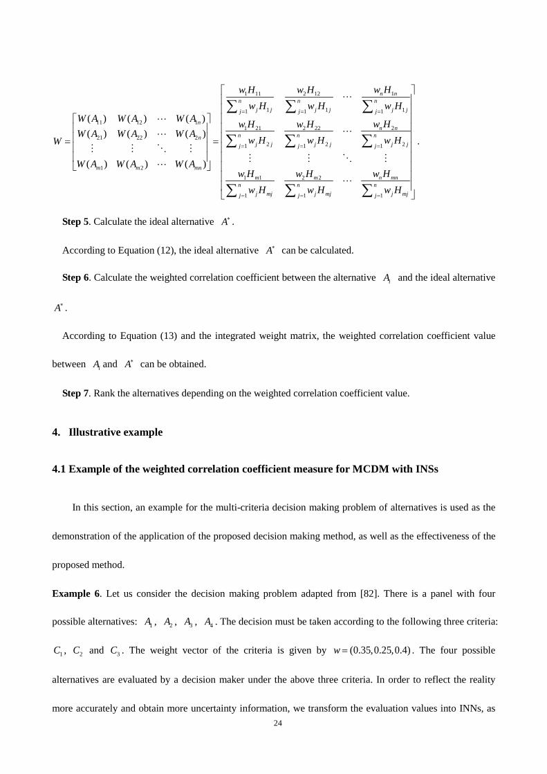
Step 5. Calculate the ideal alternative A∗ .

According to Equation (12), the ideal alternative A∗ can be calculated.

Step 6. Calculate the weighted correlation coefficient between the alternative iA and the ideal alternative

A∗ .

According to Equation (13) and the integrated weight matrix, the weighted correlation coefficient value

between iA and A∗ can be obtained.

Step 7. Rank the alternatives depending on the weighted correlation coefficient value.

4. Illustrative example

4.1 Example of the weighted correlation coefficient measure for MCDM with INSs

In this section, an example for the multi-criteria decision making problem of alternatives is used as the

demonstration of the application of the proposed decision making method, as well as the effectiveness of the

proposed method.

Example 6. Let us consider the decision making problem adapted from [82]. There is a panel with four

possible alternatives: 1A , 2A , 3A , 4A . The decision must be taken according to the following three criteria:

1C , 2C and 3C . The weight vector of the criteria is given by (0.35,0.25,0.4)w = . The four possible

alternatives are evaluated by a decision maker under the above three criteria. In order to reflect the reality

more accurately and obtain more uncertainty information, we transform the evaluation values into INNs, as

25

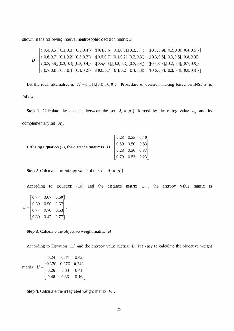
shown in the following interval neutrosophic decision matrix D:

[0.4,0.5],[0.2,0.3],[0.3,0.4] [0.4,0.6],[0.1,0.3],[0.2,0.4] [0.7,0.9],[0.2,0.3],[0.4,0.5][0.6,0.7],[0.1,0.2],[0.2,0.3] [0.6,0.7],[0.1,0.2],[0.2,0.3] [0.3,0.6],[0.3,0.5],[0.8,0.9][0.3,0.6],[

D

⟨ ⟩ ⟨ ⟩ ⟨ ⟩⟨ ⟩ ⟨ ⟩ ⟨ ⟩

=⟨ 0.2,0.3],[0.3,0.4] [0.5,0.6],[0.2,0.3],[0.3,0.4] [0.4,0.5],[0.2,0.4],[0.7,0.9][0.7,0.8],[0.0,0.1],[0.1,0.2] [0.6,0.7],[0.1,0.2],[0.1,0.3] [0.6,0.7],[0.3,0.4],[0.8,0.9]

⟩ ⟨ ⟩ ⟨ ⟩ ⟨ ⟩ ⟨ ⟩ ⟨ ⟩

Let the ideal alternative is * [1,1],[0,0],[0,0]A =< > Procedure of decision making based on INSs is as

follow.

Step 1. Calculate the distance between the set { }ij ijA a= formed by the rating value ija and its

complementary set cijA .

Utilizing Equation (2), the distance matrix is

0.23 0.33 0.400.50 0.50 0.330.23 0.30 0.370.70 0.53 0.23

D

=

.

Step 2. Calculate the entropy value of the set { }ij ijA a= .

According to Equation (10) and the distance matrix D , the entropy value matrix is

0.77 0.67 0.600.50 0.50 0.670.77 0.70 0.630.30 0.47 0.77

E

=

.

Step 3. Calculate the objective weight matrix H .

According to Equation (11) and the entropy value matrix E , it’s easy to calculate the objective weight

matrix

0.24 0.34 0.420.376 0.376 0.2480.26 0.33 0.410.48 0.36 0.16

H

=

.

Step 4. Calculate the integrated weight matrix W .

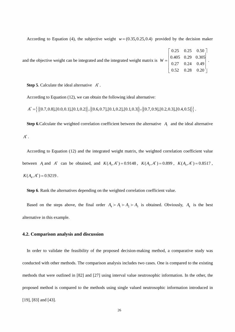
26

According to Equation (4), the subjective weight (0.35,0.25,0.4)w = provided by the decision maker

and the objective weight can be integrated and the integrated weight matrix is

0.25 0.25 0.500.405 0.29 0.3050.27 0.24 0.490.52 0.28 0.20

W

=

.

Step 5. Calculate the ideal alternative A∗ .

According to Equation (12), we can obtain the following ideal alternative:

{ }* [0.7,0.8],[0.0,0.1],[0.1,0.2] , [0.6,0.7],[0.1,0.2],[0.1,0.3] [0.7,0.9],[0.2,0.3],[0.4,0.5]A = ， .

Step 6.Calculate the weighted correlation coefficient between the alternative iA and the ideal alternative

A∗ .

According to Equation (12) and the integrated weight matrix, the weighted correlation coefficient value

between iA and A∗ can be obtained, and 1( , ) 0.9148K A A∗ = , 2( , ) 0.899K A A∗ = , 3( , ) 0.8517K A A∗ = ,

4( , ) 0.9219K A A∗ = .

Step 6. Rank the alternatives depending on the weighted correlation coefficient value.

Based on the steps above, the final order 4 1 2 3A A A A is obtained. Obviously, 4A is the best

alternative in this example.

4.2. Comparison analysis and discussion

In order to validate the feasibility of the proposed decision-making method, a comparative study was

conducted with other methods. The comparison analysis includes two cases. One is compared to the existing

methods that were outlined in [82] and [27] using interval value neutrosophic information. In the other, the

proposed method is compared to the methods using single valued neutrosophic information introduced in

[19], [83] and [43].

27

Case 1. The proposed approach is compared with some methods using interval neutrosophic information.

With regard to the method in [27], the similarity measures were calculated and used to determine the final

ranking order of all the alternatives first, and then two aggregation operators were developed in order to

aggregate the interval neutrosophic information [82]. To solve the MCDM problem in Example 6, the results

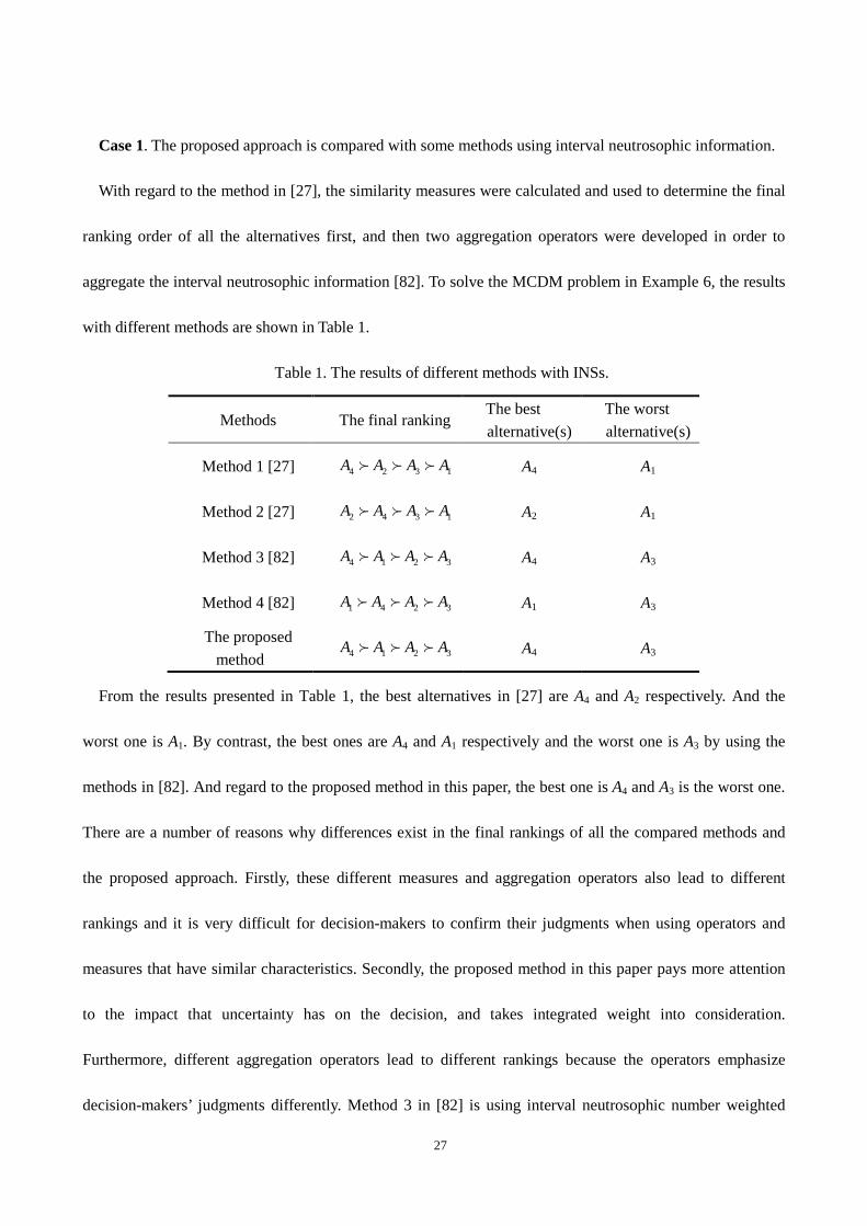
with different methods are shown in Table 1.

Table 1. The results of different methods with INSs.

Methods The final ranking The best alternative(s)

The worst alternative(s)

Method 1 [27] 4 2 3 1A A A A A4 A1

Method 2 [27] 2 4 3 1A A A A A2 A1

Method 3 [82] 4 1 2 3A A A A A4 A3

Method 4 [82] 1 4 2 3A A A A A1 A3

The proposed method 4 1 2 3A A A A A4 A3

From the results presented in Table 1, the best alternatives in [27] are A4 and A2 respectively. And the

worst one is A1. By contrast, the best ones are A4 and A1 respectively and the worst one is A3 by using the

methods in [82]. And regard to the proposed method in this paper, the best one is A4 and A3 is the worst one.

There are a number of reasons why differences exist in the final rankings of all the compared methods and

the proposed approach. Firstly, these different measures and aggregation operators also lead to different

rankings and it is very difficult for decision-makers to confirm their judgments when using operators and

measures that have similar characteristics. Secondly, the proposed method in this paper pays more attention

to the impact that uncertainty has on the decision, and takes integrated weight into consideration.

Furthermore, different aggregation operators lead to different rankings because the operators emphasize

decision-makers’ judgments differently. Method 3 in [82] is using interval neutrosophic number weighted

28

averaging (INNWA) operator and method 4 in [82] is using interval neutrosophic number weighted

geometric (INNWG) operator. The INNWA operator is based on arithmetic average and emphasizes group’s

major points while the INNWG operator emphasizes personal major points. That is the reason why results by

method 3 and method 4 in [82] are different. By comparison, the proposed method in this paper focuses on

weighted correlation coefficient measure which takes both the subjective weight and the subjective weight

into consideration. Even so, the rank by the proposed method is as same as that of INNWG operator, which

emphasizes personal major points. Therefore, the proposed method is effective.

Case 2. The proposed approach is compared with some methods using simplified neutrosophic

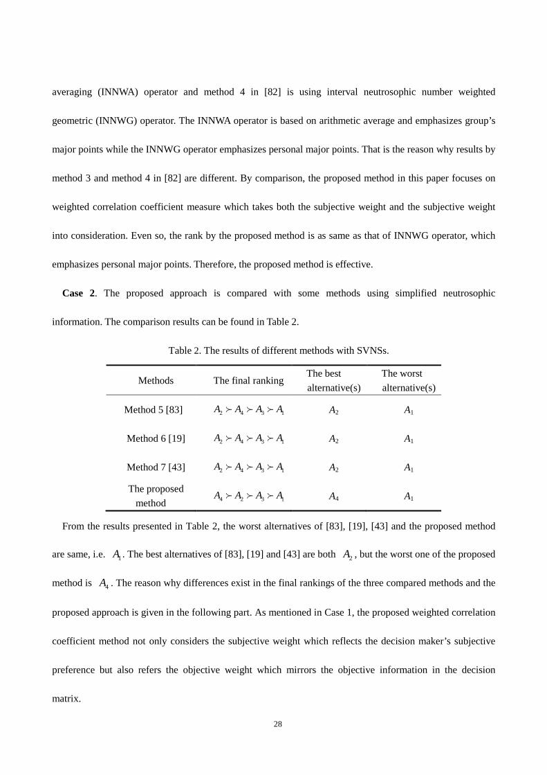
information. The comparison results can be found in Table 2.

Table 2. The results of different methods with SVNSs.

Methods The final ranking The best alternative(s)

The worst alternative(s)

Method 5 [83] 2 4 3 1A A A A A2 A1

Method 6 [19] 2 4 3 1A A A A A2 A1

Method 7 [43] 2 4 3 1A A A A A2 A1

The proposed method 4 2 3 1A A A A A4 A1

From the results presented in Table 2, the worst alternatives of [83], [19], [43] and the proposed method

are same, i.e. 1A . The best alternatives of [83], [19] and [43] are both 2A , but the worst one of the proposed

method is 4A . The reason why differences exist in the final rankings of the three compared methods and the

proposed approach is given in the following part. As mentioned in Case 1, the proposed weighted correlation

coefficient method not only considers the subjective weight which reflects the decision maker’s subjective

preference but also refers the objective weight which mirrors the objective information in the decision

matrix.

29

It shows that the proposed method can also be used to MCDM problems with single valued neutrosophic

set information.

From the comparison analysis presented above, it can be concluded that the proposed approach is more

flexible and reliable in handling MCDM problems than the compared methods in the interval neutrosophic

environment, which means that the approach developed in this paper has some advantages. Firstly, it can also

be used to solve problems with the preference information that is expressed by INSs as well as SVNSs.

Secondly, it unearths the deeper uncertainty information and utilizes them to make precise decision-making

program. Besides, it is also capable for handling the multi-criteria decision making problems with

completely unknown weight for criteria. In addition, it is utilitarian for the amount of computation can be

evidently reduced with the assistance of programming software, such as MATLAB.

5. Conclusion

NS has been applied in addressing problems with uncertain, imprecise, incomplete and inconsistent

information existing in real scientific and engineering applications. Correlation coefficient measure is

important in NS theory and entropy measure and it captures the uncertainty of NSs. Motivated by the

correlation coefficient of IFSs, a new correlation coefficient measure for INSs satisfying the property that the

value equals one if and only if two INSs are the same was proposed. Besides, the weighted correlation

coefficient measure was extended and its property was developed. Moreover, the entropy measure of INSs

was defined based on relationship among distance, similarity and entropy. As well, in order to obtain the

integrated weight, we discussed an objective weight measure utilizing entropy for INSs and established the

decision making procedure for MCDM problems. Furthermore, an illustrative example demonstrated the

application of the proposed decision making method and comparative discussions showed that the proposed

30

methods are appropriate and effective for dealing with MCDM problems.

The advantage of the proposed method is that it is simple and convenient in computing and it contributes

to decreasing the loss of evaluation information. The feasibility and validity of the proposed approach have

been verified through the illustrative example and comparison analysis. Therefore, this approach has much

application potential in dealing with issues with the interval neutrosophic information in the environment of

cluster analysis, artificial intelligence and other areas. What’s more, the new correlation coefficient measure

overcome the shortcoming that the correlation coefficient measure in [42] does not satisfy the property that

the value equals one if and only if two INSs are the same. Moreover, this paper elaborates and demonstrates

the standpoint that the uncertainty of evaluation has something to do with its importance and through

combining the subjective weight and the objective weight can avoid the non-determinacy and arbitrariness

resulted from subjective opinions. And based on these viewpoints, this paper takes further use of the

uncertainty information and proposes a weighted correlation coefficient decision making method taking both

the subjective weight and the objective weight into account which can be helpful to make wiser decision(s).

Acknowledgement

This work was supported by Humanities and Social Sciences Foundation of Ministry of Education of

China (No. 11YJCZH227) and the National Natural Science Foundation of China (Nos. 71210003 and

71221061).

References

[1] L.A. Zadeh, Fuzzy sets, Information and control, 8 (1965) 338-353. [2] R.E. Bellman, L.A. Zadeh, Decision-making in a fuzzy environment, Management science, 17 (1970) B-141-B-164. [3] R.R. Yager, Multiple objective decision-making using fuzzy sets, International Journal of Man-Machine Studies, 9 (1977) 375-382. [4] L.A. Zadeh, Probability measures of fuzzy events, Journal of mathematical analysis and applications, 23 (1968) 421-427.

31

[5] I.B. Turksen, Interval valued fuzzy sets based on normal forms, Fuzzy sets and systems, 20 (1986) 191-210. [6] K.T. Atanassov, Intuitionistic fuzzy sets, Fuzzy sets and Systems, 20 (1986) 87-96. [7] K. Atanassov, G. Gargov, Interval valued intuitionistic fuzzy sets, Fuzzy sets and systems, 31 (1989) 343-349. [8] V. Torra, Hesitant fuzzy sets, International Journal of Intelligent Systems, 25 (2010) 529-539. [9] T.K. Shinoj, J.J. Sunil, Intuitionistic fuzzy multisets and its application in medical fiagnosis, International Journal of Mathematical and Computational Sciences, 6 (2012) 34-37. [10] T. Chaira, Intuitionistic fuzzy set approach for color region extraction, Journal of Scientific & Industrial Research, 69 (2010) 426-432. [11] B.P. Joshi, S. Kumar, Fuzzy time series model based on intuitionistic fuzzy sets for empirical research in stock market, International Journal of Applied Evolutionary Computation, 3 (2012) 71-84. [12] j.-q. wang, P. Wang, J. Wang, H.-y. Zhang, X.-h. Chen, Atanassov's Interval-valued Intuitionistic Linguistic Multi-criteria Group Decision-making Method Based on Trapezium Cloud Model, IEEE Transactions on Fuzzy Systems, (2014). [13] J.-q. Wang, J.-t. Wu, J. Wang, H.-y. Zhang, X.-h. Chen, Interval-valued hesitant fuzzy linguistic sets and their applications in multi-criteria decision-making problems, Information Sciences, 288 (2014) 55-72. [14] J.-q. Wang, J.-j. Peng, H.-y. Zhang, T. Liu, X.-h. Chen, An Uncertain Linguistic Multi-criteria Group Decision-Making Method Based on a Cloud Model, Group Decision and Negotiation, 24 (2014) 171–192. [15] J.-q. Wang, L. Peng, H.-y. Zhang, X.-h. Chen, Method of multi-criteria group decision-making based on cloud aggregation operators with linguistic information, Information Sciences, 274 (2014) 177-191. [16] F. Smarandache, A unifying field in logics. Neutrosophy: Neutrosophic probability, set and logic, American Research Press, Rehoboth, 1999. [17] U. Rivieccio, Neutrosophic logics: Prospects and problems, Fuzzy Sets and Systems, 159 (2008) 1860-1868. [18] P. Majumdarar, S.K. Samant, On similarity and entropy of neutrosophic sets, Journal of Intelligent and fuzzy Systems, 26 (2014) 1245-1252. [19] J. Ye, Multicriteria decision-making method using the correlation coefficient under single-valued neutrosophic environment, International Journal of General Systems, 42 (2013) 386-394. [20] J. Ye, A multicriteria decision-making method using aggregation operators for simplified neutrosophic sets, Journal of Intelligent and fuzzy Systems, 26 (2014) 2459-2466. [21] J.-j. Peng, J.-q. Wang, H.-y. Zhang, X.-h. Chen, An outranking approach for multi-criteria decision-making problems with simplified neutrosophic sets, Applied Soft Computing, 25 (2014) 336-346. [22] P. Liu, Y. Wang, Multiple attribute decision-making method based on single-valued neutrosophic normalized weighted Bonferroni mean, Neural Computing and Applications, 25 (2014) 2001-2010. [23] H. Wang, F. Smarandache, Y.-Q. Zhang, R. Sunderraman, Interval neutrosophic sets and logic: theory and applications in computing, Hexis, Arizona, 2005. [24] F.G. Lupiáñez, Interval neutrosophic sets and topology, Kybernetes, 38 (2009) 621-624. [25] H.-y. Zhang, J.-q. Wang, X.-h. Chen, Interval Neutrosophic Sets and Their Application in Multicriteria Decision Making Problems, Scientific World Journal, (2014). [26] J. Ye, Single valued neutrosophic cross-entropy for multicriteria decision making problems, Applied Mathematical Modelling, 38 (2014) 1170-1175. [27] J. Ye, A multicriteria decision-making method using aggregation operators for simplified neutrosophic sets, Journal of Intelligent and Fuzzy Systems, 26 (2014) 2459-2466. [28] D.-A. Chiang, N.P. Lin, Correlation of fuzzy sets, Fuzzy sets and systems, 102 (1999) 221-226. [29] T. Gerstenkorn, J. Mańko, Correlation of intuitionistic fuzzy sets, Fuzzy Sets and Systems, 44 (1991) 39-43. [30] D.H. Hong, S.Y. Hwang, Correlation of intuitionistic fuzzy sets in probability spaces, Fuzzy Sets and Systems, 75

32

(1995) 77-81. [31] W.-L. Hung, J.-W. Wu, Correlation of intuitionistic fuzzy sets by centroid method, Information Sciences, 144 (2002) 219-225. [32] I. Hanafy, A. Salama, K. Mahfouz, Correlation coefficients of generalized intuitionistic fuzzy sets by centroid method, IOSR Journal of Mechanical and civil Engineering, ISSN, 3 (2012) 11-14. [33] H. Bustince, P. Burillo, Correlation of interval-valued intuitionistic fuzzy sets, Fuzzy sets and systems, 74 (1995) 237-244. [34] J. Ye, Multicriteria fuzzy decision-making method using entropy weights-based correlation coefficients of interval-valued intuitionistic fuzzy sets, Applied Mathematical Modelling, 34 (2010) 3864-3870. [35] D.G. Park, Y.C. Kwun, J.H. Park, I.Y. Park, Correlation coefficient of interval-valued intuitionistic fuzzy sets and its application to multiple attribute group decision making problems, Mathematical and Computer Modelling, 50 (2009) 1279-1293. [36] E. Szmidt, J. Kacprzyk, Correlation of intuitionistic fuzzy sets, in: Computational Intelligence for Knowledge-Based Systems Design, Springer, 2010, pp. 169-177. [37] G.-w. Wei, H.-J. Wang, R. Lin, Application of correlation coefficient to interval-valued intuitionistic fuzzy multiple attribute decision-making with incomplete weight information, Knowledge and Information Systems, 26 (2011) 337-349. [38] J.-H. Yang, M.-S. Yang, A control chart pattern recognition system using a statistical correlation coefficient method, Computers & Industrial Engineering, 48 (2005) 205-221. [39] M.A. Hall, Correlation-based feature selection for machine learning, in, The University of Waikato, 1999. [40] T. Kimoto, K. Asakawa, M. Yoda, M. Takeoka, Stock market prediction system with modular neural networks, in: Neural Networks, 1990., 1990 IJCNN International Joint Conference on, IEEE, 1990, pp. 1-6. [41] I. Hanafy, A. Salama, K. Mahfouz, Correlation of neutrosophic Data, International Refereed Journal of Engineering and Science (IRJES), 1 (2012) 39-43. [42] S. Broumi, F. Smarandache, Correlation Coefficient of Interval Neutrosophic set, Mechanical Engineering and Manufacturing, 436 (2013) 511-517. [43] J. Ye, Improved correlation coefficients of single valued neutrosophic sets and interval neutrosophic sets for multiple attribute decision making, Journal of Intelligent and Fuzzy Systems, 27 (2014) 2453-2462. [44] H.-P. Kriegel, P. Kröger, E. Schubert, A. Zimek, A general framework for increasing the robustness of PCA-based correlation clustering algorithms, in: Scientific and Statistical Database Management, Springer, 2008, pp. 418-435. [45] T.-C. Wang, H.-D. Lee, Developing a fuzzy TOPSIS approach based on subjective weights and objective weights, Expert Systems with Applications, 36 (2009) 8980-8985. [46] R.L. Keeney, H. Raiffa, Decisions with multiple objectives: preferences and value trade-offs, Cambridge university press, 1993. [47] T.L. Saaty, Modeling unstructured decision problems—the theory of analytical hierarchies, Mathematics and computers in simulation, 20 (1978) 147-158. [48] T.L. Saaty, A scaling method for priorities in hierarchical structures, Journal of mathematical psychology, 15 (1977) 234-281. [49] K. Cogger, P. Yu, Eigenweight vectors and least-distance approximation for revealed preference in pairwise weight ratios, Journal of Optimization Theory and Applications, 46 (1985) 483-491. [50] A. Chu, R. Kalaba, K. Spingarn, A comparison of two methods for determining the weights of belonging to fuzzy sets, Journal of Optimization theory and applications, 27 (1979) 531-538. [51] Y.-M. Wang, Z.-P. Fan, Z. Hua, A chi-square method for obtaining a priority vector from multiplicative and fuzzy preference relations, European Journal of Operational Research, 182 (2007) 356-366.

33

[52] D. Diakoulaki, G. Mavrotas, L. Papayannakis, Determining objective weights in multiple criteria problems: the CRITIC method, Computers & Operations Research, 22 (1995) 763-770. [53] Y. Wang, Using the method of maximizing deviations to make decision for multi-indices, System Engineering and Electronics, 7 (1998) 24-26. [54] Z. Wu, Y. Chen, The maximizing deviation method for group multiple attribute decision making under linguistic environment, Fuzzy Sets and Systems, 158 (2007) 1608-1617. [55] Z.-H. Zou, Y. Yun, J.-N. Sun, Entropy method for determination of weight of evaluating indicators in fuzzy synthetic evaluation for water quality assessment, Journal of Environmental Sciences, 18 (2006) 1020-1023. [56] J. Ma, Z.-P. Fan, L.-H. Huang, A subjective and objective integrated approach to determine attribute weights, European Journal of Operational Research, 112 (1999) 397-404. [57] Y.-M. Wang, C. Parkan, Multiple attribute decision making based on fuzzy preference information on alternatives: Ranking and weighting, Fuzzy sets and systems, 153 (2005) 331-346. [58] L. Chen, Y.-z. Wang, Research on TOPSIS integrated evaluation and decision method based on entropy coefficient, Control and decision, 18 (2003) 456-459. [59] P. Liu, X. Zhang, Research on the supplier selection of a supply chain based on entropy weight and improved ELECTRE-III method, International Journal of Production Research, 49 (2011) 637-646. [60] D.-L. Mon, C.-H. Cheng, J.-C. Lin, Evaluating weapon system using fuzzy analytic hierarchy process based on entropy weight, Fuzzy sets and systems, 62 (1994) 127-134. [61] X.-m. Meng, H.-p. Hu, Application of set pair analysis model based on entropy weight to comprehensive evaluation of water quality, Journal of Hydraulic Engineering, 3 (2009) 257-262. [62] A. De Luca, S. Termini, A definition of a nonprobabilistic entropy in the setting of fuzzy sets theory, Information and control, 20 (1972) 301-312. [63] E. Trillas, T. Riera, Entropies in finite fuzzy sets, Information Sciences, 15 (1978) 159-168. [64] R.R. Yager, On measure of fuzziness and fuzzy complements, International Journal of General Systems, 8 (1982) 169-180. [65] J. Fan, W. Xie, Distance measure and induced fuzzy entropy, Fuzzy sets and systems, 104 (1999) 305-314. [66] P. Burillo, H. Bustince, Entropy on intuitionistic fuzzy sets and on interval-valued fuzzy sets, Fuzzy sets and systems, 78 (1996) 305-316. [67] E. Szmidt, J. Kacprzyk, Entropy for intuitionistic fuzzy sets, Fuzzy sets and systems, 118 (2001) 467-477. [68] E. Szmidt, J. Kacprzyk, New measures of entropy for intuitionistic fuzzy sets, in: Ninth Int Conf IFSs Sofia, 2005, pp. 12-20. [69] P. Majumdar, S.K. Samanta, On similarity and entropy of neutrosophic sets, Journal of Intelligent and fuzzy Systems, 26 (2014) 1245-1252. [70] W. Zeng, H. Li, Relationship between similarity measure and entropy of interval valued fuzzy sets, Fuzzy Sets and Systems, 157 (2006) 1477-1484. [71] W. Zeng, P. Guo, Normalized distance, similarity measure, inclusion measure and entropy of interval-valued fuzzy sets and their relationship, Information Sciences, 178 (2008) 1334-1342. [72] X.-c. Liu, Entropy, distance measure and similarity measure of fuzzy sets and their relations, Fuzzy sets and systems, 52 (1992) 305-318. [73] J. Li, G. Deng, H. Li, W. Zeng, The relationship between similarity measure and entropy of intuitionistic fuzzy sets, Information Sciences, 188 (2012) 314-321. [74] J. Ye, Fuzzy decision-making method based on the weighted correlation coefficient under intuitionistic fuzzy environment, European Journal of Operational Research, 205 (2010) 202-204. [75] Z. Xu, J. Chen, J. Wu, Clustering algorithm for intuitionistic fuzzy sets, Information Sciences, 178 (2008)

34

3775-3790. [76] H. Wang, F. Smarandache, R. Sunderraman, Y.-Q. Zhang, Interval Neutrosophic Sets and Logic: Theory and Applications in Computing: Theory and Applications in Computing, Infinite Study, 2005. [77] F. Smarandache, Neutrosophic set-a generalization of the intuitionistic fuzzy set, in: Granular Computing, 2006 IEEE International Conference on, IEEE, 2006, pp. 38-42. [78] J. Ye, Similarity measures between interval neutrosophic sets and their applications in multicriteria decision-making, Journal of Intelligent and Fuzzy Systems, 26 (2014) 165-172. [79] Y.-q. Luo, J.-b. Xia, T.-p. Chen, Comparison of objective weight determination methods in network performance evaluation, Journal of Computer Applications, 10 (2009) 48-49. [80] H. Zhang, H. Mao, Comparison of four methods for deciding objective weights of features for classifying stored-grain insects based on extension theory, Transactions of the Chinese Society of Agricultural Engineering, 25 (2009) 132-136. [81] Y. Qi, F. Wen, K. Wang, L. Li, S. Singh, A fuzzy comprehensive evaluation and entropy weight decision-making based method for power network structure assessment, International Journal of Engineering, Science and Technology, 2 (2010) 92-99. [82] H.-y. Zhang, J.-q. Wang, X.-h. Chen, Interval neutrosophic sets and their application in multicriteria decision making problems, The Scientific World Journal, 2014 (2014). [83] R. Şahin, A. Küçük, Subsethood measure for single valued neutrosophic sets, Journal of Intelligent and Fuzzy Systems, (2014).