Improvement of the

Recognition Module of WinBank

6.199 Advanced Undergraduate Project

Daniel González MIT EECS 2002

Advisors: Professor Amar Gupta Dr. Rafael Palacios

González 2

Table of Contents 1. Introduction..............................................................................3 2. Background...............................................................................3

2.1 WinBank ..................................................................................................................... 3 2.1.1 Preprocessing Module .................................................................................................. 3 2.1.2 Recognition Module ...................................................................................................... 4 2.1.3 Postprocessing Module ................................................................................................. 4

2.2 Neural Networks .......................................................................................................... 4 3. Procedure..................................................................................6

3.1 Creation........................................................................................................................... 6 3.2 Training........................................................................................................................... 6 3.3 Testing.............................................................................................................................. 7 3.4 Evaluation....................................................................................................................... 7

4. Network Parameters ................................................................8 4.1 Neural Network Architecture.................................................................................. 8

4.1.1 Hidden Layer Size ......................................................................................................... 8 4.1.2 Network Type ................................................................................................................ 9 4.1.3 Transfer Functions........................................................................................................ 9

4.2 Neural Network Training ....................................................................................... 10 4.2.1 Performance Functions............................................................................................... 10 4.2.2 Training Algorithms.................................................................................................... 10

5. Results .....................................................................................11 5.1 Feed-Forward Network Results ........................................................................... 11

5.1.1 Hidden Layer Sizes ..................................................................................................... 12 5.1.2 Transfer Functions...................................................................................................... 13 5.1.3 Performance Functions............................................................................................... 13 5.1.4 Training Algorithms.................................................................................................... 14 5.1.5 Total Network Analysis ............................................................................................... 15

5.2 LVQ Network Results .............................................................................................. 18 5.3 Elman Network Results ........................................................................................... 18

6. Conclusion...............................................................................18 References ....................................................................................19 Appendix A: MATLAB Code ................................................20

González 3

1. Introduction More than 60 billion checks are written annually in the United States alone. The current

system for processing these checks involves human workers who read the values from the checks and enter them into a computer system. Two readers are used for each check to increase accuracy. This method of processing checks requires an enormous amount of overhead. Because such a large number of checks are written annually, even a small reduction in the cost of processing a single check adds up to significant savings. WinBank is a program that is being created to automate check processing, drastically reducing the time and money spent processing checks.

WinBank receives the scanned image of a check as input, and outputs the value for which the check was written. This process of translating physical text (in this case, hand-written numerals) into data that can be manipulated and understood by a computer is known as Optical Character Recognition (OCR). WinBank implements OCR through heavy use of a concept from artificial intelligence known as neural networks. Neural networks can be used to solve a variety of problems and are a particularly good method for solving pattern recognition problems. The effectiveness of a neural network at solving problems depends on many different network parameters, including its architecture and the process by which a network is taught to solve problems (known as training).

This paper explores the different neural network architectures considered for use in WinBank and the processes used to train them. The following section presents background information on WinBank and neural networks, and is followed by a discussion of the procedures used to test the different types of neural networks considered. This procedural information is followed by an explanation the different parameters (and their associated values) used for creating and training the networks. The next section presents the values obtained from evaluating the performances of the neural networks. The final section identifies the best neural network for use in WinBank, as well as other neural networks that may be useful in other problems.

2. Background The main focus of this paper is the module of WinBank that uses neural networks to recognize handwritten numbers. However, a brief overview of the entire WinBank system and background information on neural networks are presented here for the readers’ benefit. 2.1 WinBank

The Productivity From Information Technology Initiatives (PROFIT) group at MIT’s Sloan School of Management is developing a program called WinBank in an effort to automate check processing in both the United States and Brazil. WinBank achieves this automation by implementing OCR with a heavy dependence on neural networks. The program is organized into three main modules that combine to implement OCR. The three modules that make up WinBank are the preprocessing module, the postprocessing module, and the recognition module. 2.1.1 Preprocessing Module

The preprocessing module takes the scanned image of a check as input, and outputs binary images in a format that is useful for the recognition module. The preprocessing module first analyzes the scanned image to determine the location of the courtesy amount block (CAB). The CAB is the location on the check that contains the dollar amount of the check in Arabic numerals (figure 1). After determining the location of the CAB, the preprocessing module next attempts to segment the value written in the CAB into individual digits. These segments are then

González 4

passed through a normalization procedure designed to make all of the characters a uniform size and a uniform thickness. The preprocessed images are then individually output to the recognition module.

Figure 1: Courtesy Amount Block (CAB) Location

2.1.2 Recognition Module The recognition module is the main engine that attempts to classify the number

represented by each image received from the preprocessing module. The recognition module feeds the output obtained from the preprocessing module into a neural network. The neural network then attempts to identify the value represented by this input and outputs a number from zero to nine. 2.1.3 Postprocessing Module

The postprocessing module receives the output of the recognition module and gauges the strength of the recognition module’s guess. If the postprocessing module is not satisfied that the recognition module has output a correct value, then either the entire process begins again (making different decisions along the way) or the check is rejected and a human steps in to identify the value of the check. If the postprocessing module is satisfied with the recognition module’s output, then it outputs this value as the output of WinBank.

PreprocessingModule

CAB LocationImageSegmentationImageNormalization

RecognitionModule

NumberIdentificationBasicVerification

PostprocessingModule

DetailedVerification

Normalized ,Segmented

ImagesIdentified Number W inBank Output

Feedback

Figure 2: The three major modules of WinBank

2.2 Neural Networks Artificial neural networks are a modeled after the organic neural networks in the brain of

an organism. The fundamental unit of an organic neural network is the neuron. Neurons receive input from one or more different neurons. The strength of the effect that each input has on a neuron depends on the neuron’s proximity to the neuron from which it received the input[3]. If the combined value of these inputs is strong enough, then the neuron receiving these signals outputs a brief pulse. When neurons combine with many other neurons (there are approximately 1011 neurons in the human brain [3]) to form networks, an organism can learn to think and make decisions.

González 5

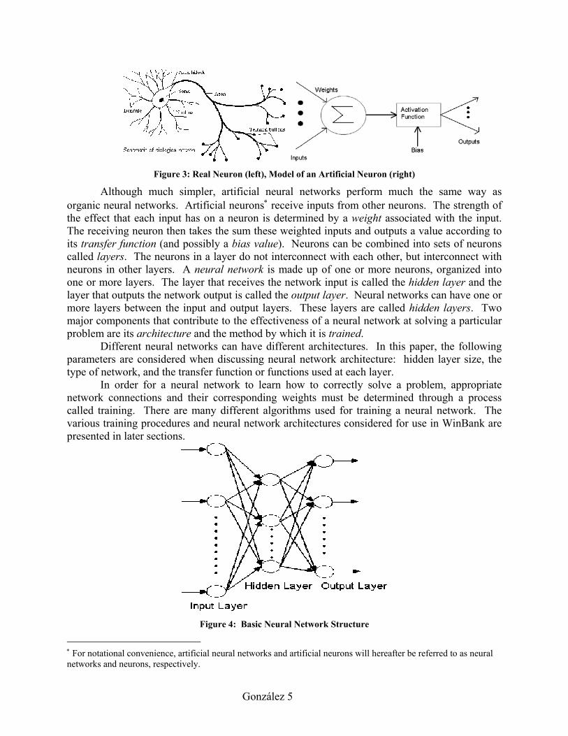
Figure 3: Real Neuron (left), Model of an Artificial Neuron (right)

Although much simpler, artificial neural networks perform much the same way as organic neural networks. Artificial neurons∗ receive inputs from other neurons. The strength of the effect that each input has on a neuron is determined by a weight associated with the input. The receiving neuron then takes the sum these weighted inputs and outputs a value according to its transfer function (and possibly a bias value). Neurons can be combined into sets of neurons called layers. The neurons in a layer do not interconnect with each other, but interconnect with neurons in other layers. A neural network is made up of one or more neurons, organized into one or more layers. The layer that receives the network input is called the hidden layer and the layer that outputs the network output is called the output layer. Neural networks can have one or more layers between the input and output layers. These layers are called hidden layers. Two major components that contribute to the effectiveness of a neural network at solving a particular problem are its architecture and the method by which it is trained.

Different neural networks can have different architectures. In this paper, the following parameters are considered when discussing neural network architecture: hidden layer size, the type of network, and the transfer function or functions used at each layer.

In order for a neural network to learn how to correctly solve a problem, appropriate network connections and their corresponding weights must be determined through a process called training. There are many different algorithms used for training a neural network. The various training procedures and neural network architectures considered for use in WinBank are presented in later sections.

Figure 4: Basic Neural Network Structure

∗ For notational convenience, artificial neural networks and artificial neurons will hereafter be referred to as neural networks and neurons, respectively.

González 6

3. Procedure Many different types of neural networks were designed, created, trained, tested, and

evaluated in an effort to find the appropriate neural network architecture and training method for use in WinBank. These networks were evaluated according to the main goal of WinBank: decrease the overhead involved in check processing as much as possible while achieving the highest possible degree of accuracy. Neural networks that decrease the overhead involved in check processing are fast and require little human intervention, while neural networks that achieve a high degree of accuracy make the fewest number of errors when classifying numbers. This section discusses the procedure used to create, train, test, and evaluate the various neural networks according to this goal.

The creation, training, and testing of each neural network was done using the MathWorks software package MATLAB. MATLAB contains a “Neural Network Toolbox” that facilitates rapid creation, training, and testing of neural networks. MATLAB was chosen to use for WinBank development because this toolbox would save an enormous amount programming effort. 3.1 Creation Creating a neural network is simply a matter of calling the appropriate MATLAB function and supplying it with the necessary information. For example, the following code creates a new feed-forward network that uses the logarithmic-sigmoidal transfer function in both layers and trains its neurons with the resilient backpropagation training algorithm: net=newff(mm, [25 10], {‘logsig’ ‘logsig’}, ‘RP’); This network has an input layer, a hidden layer consisting of 25 neurons, and an output layer consisting of 10 neurons. mm is a matrix of size number_of_inputs x 2. Each row contains the minimum and maximum value that a particular input node can have. See appendix A for more MATLAB code that can be used to create and analyze other neural networks. 3.2 Training Neural networks are useful for OCR because they can often generalize and correctly classify inputs they have not previously seen. In order reach a solid level of generalization, large amounts of data must be used during the training process. We used data from the National Institute of Standards and Technology’s (NIST) Special Database 19: Handprinted Forms and Characters Database. NIST Special Database 19 (SD19) is a database that contains Handwriting Sample Forms (HSF) from 3699 different writers (figure 5). The HSF’s each had thirty-four different fields used to gather samples of letters and numbers. Some fields were randomly generated for each HSF to obtain a larger variety of samples. Twenty-eight of the thirty-four fields were digit fields. SD19 contains scanned versions of each HSF (11.8 dots per millimeter) as well as segmented versions of the HSF’s, allowing for easy access to specific samples.

Digit samples were obtained from SD19 for use in training and testing the neural networks. Once obtained, the samples were normalized so that each sample was upright and of the same thickness∗. Some of these samples were used to create a training set and others were used to create a validation set. A training set is used to update network weights and biases, while a validation set is used to help prevent overfitting. After training, each network went through a testing procedure to gather data for evaluation of its usefulness in WinBank.

∗ For detailed information on WinBank’s normalization procedure, see [4]

González 7

Figure 5: Handwriting Sample Form from SD19

3.3 Testing Two different sets of data were obtained in order to test each network. The first set of data consisted of 10000 samples from SD19 (1000 samples per digit). These samples were presented to each network using the sim function of MATLAB. Network specific procedures were then used to compare the output of each neural network against the desired outputs. The second set of data used to test each network was a set of multiples. A multiple occurs when image segmentation fails to recognize two adjacent numbers as individual numbers and presents the recognition module with one image of two numbers (figure 6). Because a multiple is not a number, a multiple should be sent back to the preprocessing module for resegmentation. In order to test the different neural networks on multiples, multiples from several checks were used to create a testing set of multiples.

Figure 6: Example of a multiple (double zero)

3.4 Evaluation Running a network simulation in MATLAB produces a matrix of outputs. This matrix of actual network outputs can be compared to a target matrix of desired network outputs to evaluate the performance of each network. Here, the main goal of WinBank should be divided into its two components: the accuracy of a network, and its ability to reduce processing overhead. Several parameters were obtained from each network test to evaluate the performance of each network according to these goals. The percentage of correct outputs (GOOD), the percentage of incorrect outputs (WRONG), and the percentage of rejected outputs (REJECT) were obtained from the SD19 test set. The ideal network maximizes GOOD while minimizing REJECT and WRONG. MULTIPLES REJECTED and NUMBER are two parameters obtained

González 8

from testing the networks on the testing set of multiples. MULTIPLES REJECTED is the percentage of multiples rejected by the network, and should be maximized. NUMBER is the percentage of multiples classified as numbers, and should be minimized. Another useful values for network evaluation is the amount of time spent training it.

Important data for each neural network trained and tested was maintained in a MATLAB struct array named netData. Each netData struct array has fields for the each important value, such as the training time (obtained using MATLAB’s tic and toc functions) and hidden layer size of the network. This struct array allowed for easy storage and access to important information.

4. Network Parameters The following parameters were varied during the creation and training of the neural networks:

1. hidden layer size a. 25 b. 50 c. 85

2. network type a. feed-forward b. learning vector quantization c. Elman

3. transfer function used at network layers a. logarithmic-sigmoidal b. tangential-sigmoidal c. hard limit d. linear e. competitive

4. performance function a. least mean of squared errors b. least sum of squared errors

5. training algorithm a. batch gradient descent with momentum b. resilient backpropagation c. BFGS d. Levenberg-Marquardt e. random

4.1 Neural Network Architecture 4.1.1 Hidden Layer Size

Each neural network tested for use in WinBank had the same base structure. The input layer consisted of 117 nodes that receive input from the preprocessing module. These nodes correspond to the 13 x 9 pixels of the normalized binary image produced by the preprocessing module. The output layer consisted 10 nodes, the output of which is ideally high at the output node corresponding to the appropriate digit, and low at every other output node. The hidden layer structure, however, is architecture dependent. The number of hidden layers is not an important factor in the performance of a network because it has been rigorously proven one hidden layer can match the performance achieved with any number of hidden layers [2].

González 9

Because of this, all of the neural networks tested were implemented using only one hidden layer. The size of the hidden layer, however, is an important factor. Three values were tested for the number of nodes in the hidden layer of each neural network architecture: 25, 50, and 80. These values were obtained based on previous experience, and provide a diverse group of values without creating excessive computation.

Figure 7: Basic Neural Network Architecture

4.1.2 Network Type There are a variety of network types that can be used when creating neural networks. The network type can determine various network parameters, such as the type of neurons that are present in each layer and the method by which network layers are interconnected. Past experience indicates that feed-forward networks work very well for OCR. Because of this, much more time was spent analyzing feed-forward network networks than any other networks. The following types were evaluated for use in WinBank:

1. Feed-forward neural networks (also known as multi-layer perceptrons) are made up of two or more layers of neurons. The output of each layer is simply fed into the next layer, hence the name feed-forward networks. Each layer can have a different transfer function and size.

2. Learning Vector Quantization (LVQ) networks consist of an input layer, a hidden competitive layer, and an output linear layer. Competitive layers output zero for all neurons except for the neuron that is associated with the most positive element of the net input, which outputs one. The linear layer transforms the competitive layer’s output into target classifications defined by the user [1].

3. Elman networks are a type of recurrent network that consists of two feed-forward layers and have feedback from the first layer’s output to the first layer’s input. The neurons of the hidden layer have a tangential-sigmoidal transfer function, and the neurons of the output layer have a linear transfer function [1].

4.1.3 Transfer Functions Each neuron uses a transfer function in order to determine its output based on its input. The following five transfer functions have been tested for use in WinBank:

González 10

1. The logarithmic-sigmoidal transfer function takes an input valued between negative infinity and positive infinity and outputs a value between zero and positive one.

2. The tangential-sigmoidal transfer function takes an input valued between negative infinity and positive infinity and outputs a value between negative one and positive one.

3. The hard limit transfer function outputs zero if the net input of a neuron is less than zero, and outputs one if the net input of a neuron is greater than or equal to zero.

4. The linear transfer function produces a linear mapping of input to output. 5. The competitive transfer function is used in competitive learning and accepts a net

input vector for a layer and returns neuron outputs of zero for all neurons except for the winner, the neuron associated with the most positive element of the net input [1].

4.2 Neural Network Training Two important training parameters that effect neural network performance are the performance function and the training algorithm. 4.2.1 Performance Functions Performance functions are used in supervised learning to help update the network weights and biases. In supervised learning, a network is provided with the desired output for each input. All of the neural networks tested for use in WinBank were trained using supervised learning. The error is defined as the difference between the desired output and the actual network output. Network weights in WinBank are updated according to one of two performance functions to reduce the network error:

1. Least mean of squared errors (MSE): minimizes the average of the squared network errors.

2. Least sum of squared errors (SSE): minimizes the sums of the squared network errors. 4.2.2 Training Algorithms There are many different algorithms that can be used to train a neural network. All of the training algorithms that follow are backpropagation algorithms that implement batch training. Training algorithms that use backpropagation begin by calculating the changes in the weights of the final layer before proceeding to compute the weights for the previous layer. They continue in this backwards fashion until reaching the input layer. The procedure used to compute the changes in the input weights for each node is specific to each algorithm, and there are there are various trade-offs in speed, memory consumption, and accuracy associated with each algorithm.

Algorithms that implement batch training wait until each input is present at the input layer before making any changes to the network weights. Once all of the inputs have been presented, the training algorithm modifies the weights according to its procedure. Each iteration of these algorithms is called an epoch.

The following methods were tested on one or more architectures for use in WinBank: 1. Batch Gradient Descent with Momentum training algorithm (GDM): This training

algorithm updates the network weights in the direction of the negative gradient of the performance function by a factor determined by a parameter known as the learning rate. This algorithm makes use of momentum, which allows a network to respond not only to the local gradient, but also to recent trends in the error surface, allowing networks to avoid getting stuck in shallow minima [1].

González 11

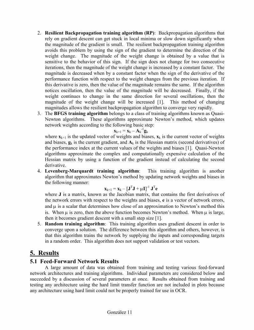
2. Resilient Backpropagation training algorithm (RP): Backpropagation algorithms that rely on gradient descent can get stuck in local minima or slow down significantly when the magnitude of the gradient is small. The resilient backpropagation training algorithm avoids this problem by using the sign of the gradient to determine the direction of the weight change. The magnitude of the weight change is obtained by a value that is sensitive to the behavior of this sign. If the sign does not change for two consecutive iterations, then the magnitude of the weight change is increased by a constant factor. The magnitude is decreased when by a constant factor when the sign of the derivative of the performance function with respect to the weight changes from the previous iteration. If this derivative is zero, then the value of the magnitude remains the same. If the algorithm notices oscillation, then the value of the magnitude will be decreased. Finally, if the weight continues to change in the same direction for several oscillations, then the magnitude of the weight change will be increased [1]. This method of changing magnitudes allows the resilient backpropagation algorithm to converge very rapidly.

3. The BFGS training algorithm belongs to a class of training algorithms known as Quasi-Newton algorithms. These algorithms approximate Newton’s method, which updates network weights according to the following basic step:

xk+1 = xk – Ak-1gk

where xk+1 is the updated vector of weights and biases, xk is the current vector of weights and biases, gk is the current gradient, and Ak is the Hessian matrix (second derivatives) of the performance index at the current values of the weights and biases [1]. Quasi-Newton algorithms approximate the complex and computationally expensive calculation of the Hessian matrix by using a function of the gradient instead of calculating the second derivative.

4. Levenberg-Marquardt training algorithm: This training algorithm is another algorithm that approximates Newton’s method by updating network weights and biases in the following manner:

xk+1 = xk – [JTJ + µI]-1 JTe where J is a matrix, known as the Jacobian matrix, that contains the first derivatives of the network errors with respect to the weights and biases, e is a vector of network errors, and µ is a scalar that determines how close of an approximation to Newton’s method this is. When µ is zero, then the above function becomes Newton’s method. When µ is large, then it becomes gradient descent with a small step size [1].

5. Random training algorithm: This training algorithm uses gradient descent in order to converge upon a solution. The difference between this algorithm and others, however, is that this algorithm trains the network by supplying the inputs and corresponding targets in a random order. This algorithm does not support validation or test vectors.

5. Results 5.1 Feed-Forward Network Results A large amount of data was obtained from training and testing various feed-forward network architectures and training algorithms. Individual parameters are considered below and succeeded by a discussion of several parameters at once. Results obtained from training and testing any architecture using the hard limit transfer function are not included in plots because any architecture using hard limit could not be properly trained for use in OCR.

González 12

Data is presented for each of the two test sets. The important parameters associated with SD19 test data are the accuracy and the rejection rate. The accuracy is the percentage of properly recognized inputs. The rejection rate is the percentage of inputs that could not be recognized by the neural network and had to be sent for further processing (either by humans or computers). The important parameters associated with the test set containing multiples are multiples rejected and multiples classified as numbers. Multiples rejected is the percentage of inputs that the network cannot recognize and rejects. Multiples classified as numbers is the percentage of inputs that the network classifies as a number. The training time is a parameter independent of test data and is the number of seconds spent training a particular network. The testing time was obtained for each network, but these times were all very similar and will not be discussed further. 5.1.1 Hidden Layer Sizes Each feed-forward network architecture was tested with three different hidden layer sizes. The different sizes were 25 nodes, 50 nodes, and 85 nodes. The results for each test set are shown below.

Figure 8: Results from feed-forward networks trained with varying hidden layer sizes and tested on properly

segmented and normalized images.

Figure 9: Results from feed-forward networks trained with varying hidden layer sizes and tested on images

of multiples.

González 13

5.1.2 Transfer Functions Each neural network architecture was trained and tested using the tangential-sigmoidal, logarithmic-sigmoidal, and hard limit transfer functions. Network architectures that used the hard limit transfer function implemented it in the output layer and the architectures were trained and tested with either the logarithmic-sigmoidal or tangential-sigmoidal transfer functions in use for the neurons of the hidden layer. No useful testing resulted from networks trained with the hard limit transfer function. Each of these networks identified every input presented as the number one. This occurs because feed-forward networks need differentiable transfer functions during training. Data associated with networks using the hard limit transfer function are thus omitted from the graphs of this section.

Figure 10: Results from feed-forward networks trained with two different transfer functions and tested on

properly segmented and normalized images.

Figure 11: Results from feed-forward networks trained with two different transfer functions and tested on

images of multiples.

5.1.3 Performance Functions Each of the feed-forward neural network architectures was trained with both the least mean squared error (MSE) and least sum of squared error (SSE) performance functions.

González 14

Figure 12: Results from feed-forward networks trained with two different performance functions and tested

on properly segmented and normalized images.

Figure 13: Results from feed-forward networks trained with two different performance functions and tested

on images of multiples.

5.1.4 Training Algorithms Each of the feed-forward network architectures were trained and tested thoroughly with both the batch gradient descent with momentum (GDM) and resilient backpropagation (RP) training algorithms. However, the BFGS (trainbfg) and Levenberg-Marquardt (trainlm) training algorithms could not be trained due to unacceptable training time and memory usage. It took trainlm seventeen minutes to train a network with a training set of one sample. Any increase of the hidden layer’s size beyond twenty-five neurons yielded and “out of memory” error, despite experimentation with the memory reduction parameter. Similar results were obtained from training and testing networks using trainbfg thus, training and testing of architectures using trainlm and trainbfg was aborted. However, tests of networks trained with GDM and RP yielded useful results, displayed in the graphs below.

González 15

Figure 14: Results from feed-forward networks trained with two different training algorithms and tested on

properly segmented and normalized images.

Figure 15: Results from feed-forward networks trained with two different training algorithms and tested on

images of multiples.

5.1.5 Total Network Analysis The network parameters considered individually above are now taken together in an effort to find the neural network parameters that best suit the goals of WinBank. The graphs below plot the rejection rate against the percentage of incorrect outputs and accuracy, respectively, of networks tested with SD19 test data. The ideal neural network in figure 16 is located as close to the origin of the left graph as possible, and as close to the top left corner of the right graph as possible. These locations minimize the rejection rate and maximize the correct output. A high accuracy rate is desirable because of the cost and inconvenience of inaccurate check values being entered into a computer system. A low rejection rate is desirable because a high rejection rate means high human intervention, increasing check processing overhead. Because the ideal neural network does not exist, a compromise must be made between these two rates. High accuracy thus becomes somewhat more desirable than a low rejection rate.

González 16

Figure 17: Two useful graphs for evaluating network performance on SD19 test inputs. Each node on the

plot corresponds to a neural network.

The input to the neural network will not always be properly segmented and normalized images such as those used to evaluate the accuracy and rejection parameters above. It is very likely that at some time the neural network will receive an image of a multiple as input. The ideal neural network will either reject the image of a multiple, or not classify it as a number. Unfortunately, the neural networks best suited to receive and classify properly normalized and segmented images are not the same neural networks best suited to receive and properly deal with images of multiples. Tables 1 and 2 contain values obtained from the best networks for evaluating proper input and multiples, respectively. The top ten networks for handling appropriately segmented and normalized data classify, on average, 72 percent of inputs that are multiples as numbers, while only rejecting an average of 24 percent of the multiples. On the other hand, the top ten networks at handling inputs that are multiples reject an average of 76 percent of proper data and only correctly classify an average of 19 percent of these data. Because of these network differences, a simple tradeoff must be made. Because a good segmentation module should be able to produce more proper inputs than improper inputs, and because the networks equipped to handle multiples are all but useless when handling proper inputs, a network is chosen that is better equipped to handle the proper inputs than multiples.

Table 1: Top ten feed-forward networks according to highest GOOD % and lowest REJECT %

GOOD % REJECT % WRONG % REJECT (MULT)% NUMBER % 85.88 10.48 3.64 33.33 66.6785.81 10.46 3.73 33.33 66.6785.29 11.16 3.55 18.18 81.8284.74 12.32 2.94 36.36 63.6479.17 18.13 2.7 39.39 60.6175.61 18.89 5.5 18.18 81.8273.49 21.13 5.38 15.15 84.8573.21 23.85 2.94 27.27 72.7371.67 23.61 4.72 21.21 78.7970.51 26.55 2.94 30.30 69.70

González 17

Table 2: Top ten feed-forward networks according to highest REJECT (MULT)%

GOOD % REJECT % WRONG % REJECT (MULT)%NUMBER %1.91 93.59 4.5 100.00 0.00

0 100 0 100.00 0.000.02 99.97 0.01 100.00 0.00

30.32 69.21 0.47 84.85 15.1513.49 78.75 7.76 81.82 18.1824.59 73.94 1.47 81.82 18.1811.1 79.14 9.76 69.70 30.30

30.56 54.97 14.47 60.61 39.3926.89 71.97 1.14 57.58 42.4254.13 40.86 5.01 54.55 45.45

From the data in table 3, networks one through four have comparable parameters, except network one has a training time that is an order of magnitude smaller than those of networks three through four. Because network weights are initialized randomly, running the same procedure with the same data more than once can produce data that is slightly different. Because of this variation, parameters that have similar values are considered to be the same. Table 3: Feed-Forward Networks Sorted by descending GOOD% and ascending REJECT%

Network TRAIN TIME

GOOD % REJECT % WRONG %

REJECT (MULT)% NUMBER %

1 2036 85.88 10.48 3.64 33.33 66.672 13361 85.81 10.46 3.73 33.33 66.673 18569 85.29 11.16 3.55 18.18 81.824 19326 84.74 12.32 2.94 36.36 63.645 3179 79.17 18.13 2.7 39.39 60.616 1131 75.61 18.89 5.5 18.18 81.827 861 73.49 21.13 5.38 15.15 84.858 1310 73.21 23.85 2.94 27.27 72.739 930 71.67 23.61 4.72 21.21 78.79

10 1192 70.51 26.55 2.94 30.30 69.7011 658 70.08 22.6 7.32 30.30 69.7012 8270 62.39 15.29 22.32 45.45 54.5513 5715 54.13 40.86 5.01 54.55 45.4514 1610 30.56 54.97 14.47 60.61 39.3915 1399 30.32 69.21 0.47 84.85 15.1516 2036 26.89 71.97 1.14 57.58 42.4217 2255 24.59 73.94 1.47 81.82 18.1818 5225 18.19 74.46 7.35 42.42 57.5819 1421 13.49 78.75 7.76 81.82 18.18

González 18

20 1277 11.48 64.56 23.96 45.45 54.5521 4129 11.1 79.14 9.76 69.70 30.3022 1946 1.91 93.59 4.5 100.00 0.0023 19452 0.02 99.97 0.01 100.00 0.0024 5039 0 100 0 100.00 0.00

Networks seven and eleven have parameters that may not necessarily differ significantly from network one, and their training times are one order of magnitude smaller than that of network one. The remaining networks differ significantly from these networks and are not considered for use in WinBank. Table three contains the network parameters associated with networks one, seven, and eleven.

Table 4: Network parameters associated with top three feed-forward networks

Network Training Algorithm

PerformanceFunction Hidden Layer Size

TransferFunction

Training Time

1 GDM SSE 50 logsig 2036 2 RP SSE 25 logsig 861 3 RP MSE 25 logsig 658

5.2 LVQ Network Results

A small number of LVQ networks were tested to compare with feed-forward networks. The top network results obtained is shown in table 5. Although the accuracy is fairly high, its inability to reject outputs leads to a high percentage of incorrect outputs. It is unable to reject outputs because LVQ networks produce binary output. Its inability to reject outputs and relatively long training time made it impractical to further pursue the use of LVQ networks.

Table 5: Top LVQ network results

Performance Function

Hidden Layer Size

train time Accuracy Reject Wrong

MSE 50 6475.88 73 0 27 5.3 Elman Network Results A small number of Elman networks were tested. Table 6 contains results from the best Elman network produced. Low accuracy and high training time were the reasons that further testing of Elman networks were abandoned.

Table 6: Top Elman network results

Performance Function

Hidden Layer Size

Layer 1Transfer Function

Layer 2Transfer Function

Train time Accuracy Reject Wrong

MSE 50 logsig logsig 8091.24 21.18 0 78.82

6. Conclusion The top network for use in WinBank is a network with a hidden layer size of 50 nodes, use the logarithmic-sigmoidal transfer function at the hidden and output layers, and uses the GDM training algorithm in combination with SSE. This combination took 2036 seconds to train and achieved an accuracy of 85 percent, while only rejecting 10 percent of its outputs. Although

González 19

the networks of table 4 produce similar output and take much less time to train, they are approximately 15 percent less accurate and reject approximately 10 percent more outputs. It is unlikely that the network will need to be retrained very often, making the larger training time of network 1 in table 4 insignificant. If the application should change and require the network to be trained more often, then the top three networks should be tested several times and be evaluated according to the averages of the values obtained. This increases the usefulness of small differences in the values obtained from testing enabling the appropriate network to be chosen. However, because network training does not currently need to occur often, network 1 in table 4 is the best network to use in WinBank.

References

[1] Demuth, Howard and Beale, Mark. “Neural Network Toolbox” (2001)

[2] Sinha, Anshu. “An Improved Recognition Module for the Identification of Handwritten

Digits” Master Thesis, Massachusetts Institute of Technology. (1999)

[3] Winston, Patrick. “Artificial Intelligence” (1992)

[4] Palacios, Rafael and Gupta, Amar. “A System for Processing Handwritten Bank Checks

Automatically” Working paper 4346-02

González 20

Appendix A: MATLAB Code The following functions can be used to create, train, and test the neural networks

described above. For more information, see the Neural Network Toolbox [1]. Creation Feed-Forward Networks newff(mm, sizeArray, transferFunctionCellArray, trainingAlgorithm); LVQ Networks newlvq(mm, hiddenLayerSize, percentages); Elman Networks newelm(mm, sizeArray, transferFunctionCellArray); mm: Matrix of size number_of_inputs x 2. Each row contains the minimum and maximum value that a particular input node can have. sizeArray: array that contains size for each layer (not including input) transferFunctionCellArray: Cell Array that contains strings representing the transfer functions for each layer (not including input layer).

Transfer function MATLAB String logarithmic-sigmoidal logsig tangential-sigmoidal tansig hard limit hardlim linear purelin competitive (automatic for appropriate layer)

trainingAlgorithm: A string representing the training algorithm for the network. Training algorithm MATLAB String Batch Gradient Descent with Momentum traingdm Resilient Backpropagation trainrp BFGS trainbfg Levenberg-Marquardt trainlm Random trainr

hiddenLayerSize: The size of the hidden layer percentages: matrix of expected percentages of inputs. Training [net, tr] = train(net, trainData, T, [], [], VV); net: neural network to be trained trainData: training data set T: desired output for each input VV: struct array of with validation inputs and targets Testing output = sim(net, testData); net: neural network to be tested testData: testing data set