Brigham Young UniversityBYU ScholarsArchive

All Theses and Dissertations

2017-04-01

Improvements, Algorithms and a SimulationModel for a Compact Phased-Array Radar for UASSense and AvoidAdam Kaleo RobertsBrigham Young University

Follow this and additional works at: https://scholarsarchive.byu.edu/etd

Part of the Electrical and Computer Engineering Commons

This Thesis is brought to you for free and open access by BYU ScholarsArchive. It has been accepted for inclusion in All Theses and Dissertations by anauthorized administrator of BYU ScholarsArchive. For more information, please contact scholarsarchive@byu.edu, ellen_amatangelo@byu.edu.

BYU ScholarsArchive CitationRoberts, Adam Kaleo, "Improvements, Algorithms and a Simulation Model for a Compact Phased-Array Radar for UAS Sense andAvoid" (2017). All Theses and Dissertations. 6314.https://scholarsarchive.byu.edu/etd/6314

Improvements, Algorithms and a Simulation Model

for a Compact Phased-Array Radar

for UAS Sense and Avoid

Adam Kaleo Roberts

A thesis submitted to the faculty of

Brigham Young University

in partial fulfillment of the requirements for the degree of

Master of Science

Karl F. Warnick, Chair

Michael D. Rice

David G. Long

Department of Electrical and Computer Engineering

Brigham Young University

Copyright c© 2017 Adam Kaleo Roberts

All Rights Reserved

ABSTRACT

Improvements, Algorithms and a Simulation Model

for a Compact Phased-Array Radar

for UAS Sense and Avoid

Adam Kaleo Roberts

Department of Electrical and Computer Engineering, BYU

Master of Science

Unmanned aerial systems (UAS) are an influential technology which can enhance life in

multiple ways. However, they must be able to sense and operate safely with manned aircraft. Radar

is an attractive sensor for UAS because of its all-weather performance. It is challenging, though, to

meet the size, weight, and power (SWaP) limitations of UAS and especially small-UAS while still

maintaining the needed sensing capability. A working FMCW radar prototype has been created

which meets the SWaP requirement of small-UAS. A simulation model for the radar was developed

to test the processing algorithms of the radar and proved to be advantageous in that purpose. An

automatic target detection algorithm was also successfully developed to allow the radar to identify

targets of interest in a cluttered and dynamic environment. Fixed-wing airborne tests have been

performed with the radar which show that the radar meets the SWaP requirements of small-UAS.

They also show the prototype requires a higher sensitivity to detect other small-UAS. A successful

redesign of the radar’s receivers was done to make the radar more sensitive.

Keywords: Sense and Avoid, Radar, FMCW Radar, Automatic Target Detection, SAFE Database

ACKNOWLEDGMENTS

I would like to thank my fellow students on this project, namely Jonthan Spencer, Michael

Boren, David Buck, and Thomas Cheney. It has been a pleasure to engage with them on the

challenges of this project. Thanks also to Luke Newmeyer and Jared Wilke for their help and

expertise in collaborating on this project.

I would like to thank my committee members Dr. Michael Rice and Dr. David Long for

their help and advice. I also want to thank my adviser Dr. Karl Warnick for his guidance and

assistance on this project over the years in which I have been a part of it.

Finally, I wish to thank my family and parents for their support and encouragement through-

out the course of my graduate experience.

TABLE OF CONTENTS

LIST OF TABLES . . . . . . . . . . . . . . . . . . . . . . . . . . . . . . . . . . . . . . . vi

LIST OF FIGURES . . . . . . . . . . . . . . . . . . . . . . . . . . . . . . . . . . . . . . vii

Chapter 1 Introduction . . . . . . . . . . . . . . . . . . . . . . . . . . . . . . . . . . . 11.1 Motivation . . . . . . . . . . . . . . . . . . . . . . . . . . . . . . . . . . . . . . . 1

1.2 Previous Work . . . . . . . . . . . . . . . . . . . . . . . . . . . . . . . . . . . . . 2

1.3 Contributions . . . . . . . . . . . . . . . . . . . . . . . . . . . . . . . . . . . . . 3

1.4 Thesis Outline . . . . . . . . . . . . . . . . . . . . . . . . . . . . . . . . . . . . . 4

Chapter 2 Background . . . . . . . . . . . . . . . . . . . . . . . . . . . . . . . . . . . 52.1 FMCW Radar . . . . . . . . . . . . . . . . . . . . . . . . . . . . . . . . . . . . . 5

2.2 Radar Performance . . . . . . . . . . . . . . . . . . . . . . . . . . . . . . . . . . 6

2.2.1 Received Power . . . . . . . . . . . . . . . . . . . . . . . . . . . . . . . . 6

2.2.2 Signal, Noise and Signal to Noise Ratio . . . . . . . . . . . . . . . . . . . 6

2.3 Noise and Random Variables . . . . . . . . . . . . . . . . . . . . . . . . . . . . . 7

2.4 Summary . . . . . . . . . . . . . . . . . . . . . . . . . . . . . . . . . . . . . . . 9

Chapter 3 Radar Hardware Design . . . . . . . . . . . . . . . . . . . . . . . . . . . . 103.1 Radar Design Overview . . . . . . . . . . . . . . . . . . . . . . . . . . . . . . . . 10

3.1.1 Transmitter . . . . . . . . . . . . . . . . . . . . . . . . . . . . . . . . . . 12

3.1.2 RF Receiver . . . . . . . . . . . . . . . . . . . . . . . . . . . . . . . . . . 13

3.1.3 IF Receiver . . . . . . . . . . . . . . . . . . . . . . . . . . . . . . . . . . 15

3.2 Receiver Dynamic Range Improvement . . . . . . . . . . . . . . . . . . . . . . . 17

3.2.1 Design Changes . . . . . . . . . . . . . . . . . . . . . . . . . . . . . . . 17

3.2.2 Measured Design Performance . . . . . . . . . . . . . . . . . . . . . . . . 19

3.3 Summary . . . . . . . . . . . . . . . . . . . . . . . . . . . . . . . . . . . . . . . 21

Chapter 4 FMCW Radar Signal Processing on a Low SWaP Platform . . . . . . . . 224.1 Signal Processing Overview . . . . . . . . . . . . . . . . . . . . . . . . . . . . . 22

4.1.1 Signal Processing Platform . . . . . . . . . . . . . . . . . . . . . . . . . . 23

4.2 Signal Digitization and Fourier Transform . . . . . . . . . . . . . . . . . . . . . . 24

4.3 Correlation and Averaging . . . . . . . . . . . . . . . . . . . . . . . . . . . . . . 26

4.4 Automatic Target Detection . . . . . . . . . . . . . . . . . . . . . . . . . . . . . . 27

4.4.1 OS-CFAR . . . . . . . . . . . . . . . . . . . . . . . . . . . . . . . . . . . 29

4.5 Clustering . . . . . . . . . . . . . . . . . . . . . . . . . . . . . . . . . . . . . . . 35

4.6 Beamforming . . . . . . . . . . . . . . . . . . . . . . . . . . . . . . . . . . . . . 36

4.7 Tracking and Collision Avoidance Processing . . . . . . . . . . . . . . . . . . . . 37

4.8 Summary . . . . . . . . . . . . . . . . . . . . . . . . . . . . . . . . . . . . . . . 37

Chapter 5 A Simulation Model for a Low SWaP FMCW Radar . . . . . . . . . . . . 395.1 Noise and Signal Power . . . . . . . . . . . . . . . . . . . . . . . . . . . . . . . . 39

iv

5.1.1 Worked Example . . . . . . . . . . . . . . . . . . . . . . . . . . . . . . . 39

5.2 Maximum Detection Range and RCS . . . . . . . . . . . . . . . . . . . . . . . . . 40

5.3 1D Phased Array Radar Model . . . . . . . . . . . . . . . . . . . . . . . . . . . . 42

5.3.1 Antenna Model . . . . . . . . . . . . . . . . . . . . . . . . . . . . . . . . 44

5.3.2 Phased Array Propagation Model . . . . . . . . . . . . . . . . . . . . . . 44

5.4 Summary . . . . . . . . . . . . . . . . . . . . . . . . . . . . . . . . . . . . . . . 45

Chapter 6 Experimental Results . . . . . . . . . . . . . . . . . . . . . . . . . . . . . . 466.1 Radar Calibration . . . . . . . . . . . . . . . . . . . . . . . . . . . . . . . . . . . 46

6.1.1 Calibration Experimental Results and Model Comparison . . . . . . . . . 46

6.2 SAFE-Database Project . . . . . . . . . . . . . . . . . . . . . . . . . . . . . . . . 49

6.2.1 Equipment Setup . . . . . . . . . . . . . . . . . . . . . . . . . . . . . . . 49

6.2.2 Flight Campaign Description . . . . . . . . . . . . . . . . . . . . . . . . . 50

6.2.3 Flight Campaign Results . . . . . . . . . . . . . . . . . . . . . . . . . . . 51

6.2.4 Preliminary Results from Design Changes . . . . . . . . . . . . . . . . . . 54

6.3 Summary . . . . . . . . . . . . . . . . . . . . . . . . . . . . . . . . . . . . . . . 55

Chapter 7 Conclusion . . . . . . . . . . . . . . . . . . . . . . . . . . . . . . . . . . . 577.1 Future Work . . . . . . . . . . . . . . . . . . . . . . . . . . . . . . . . . . . . . . 58

REFERENCES . . . . . . . . . . . . . . . . . . . . . . . . . . . . . . . . . . . . . . . . . 60

v

LIST OF TABLES

3.1 Radar Transceiver Specifications [12] . . . . . . . . . . . . . . . . . . . . . . . . . . 10

3.2 Calculated Results of Design Changes . . . . . . . . . . . . . . . . . . . . . . . . . . 19

3.3 Measured Receiver Specifications . . . . . . . . . . . . . . . . . . . . . . . . . . . . 20

3.4 Measured Receiver Saturation Performance . . . . . . . . . . . . . . . . . . . . . . . 20

5.1 Radar Specifications for Calculating the Maximum Range . . . . . . . . . . . . . . . 41

vi

LIST OF FIGURES

3.1 Completed radar system and block diagram. . . . . . . . . . . . . . . . . . . . . . 11

3.2 A spectrogram of the radar’s transmit waveform and a picture of the power amplifier

for the radar. . . . . . . . . . . . . . . . . . . . . . . . . . . . . . . . . . . . . . . 12

3.3 Planar Vivaldi antenna used as both the transmit antenna and the receiver antennas

for the radar [12]. . . . . . . . . . . . . . . . . . . . . . . . . . . . . . . . . . . . 13

3.4 The RF board. The PLL section is located on the far right of the board with the four

receiver channels located on the left. The Wilkinson splitter network occupies the

middle-left of the board. This figure shows the new receiver design of Section 3.2 . 14

3.5 IF Circuit schematic of a single channel [12] . . . . . . . . . . . . . . . . . . . . . 15

3.6 The IF board. The design of each channel is identical. . . . . . . . . . . . . . . . . 16

3.7 IF circuit simulated frequency response [12] . . . . . . . . . . . . . . . . . . . . . 17

3.8 Previous and new receiver chain designs . . . . . . . . . . . . . . . . . . . . . . . 18

4.1 Block diagram of the DSP system. . . . . . . . . . . . . . . . . . . . . . . . . . . 23

4.2 The MicroZed (left) and BOARAC (right) boards. The MicroZed houses the FPGA

and processor for signal processing while ADCs are located on the BOARAC board

which perform the sampling [12]. . . . . . . . . . . . . . . . . . . . . . . . . . . . 24

4.3 Illustration of the relationship between the sampling blocks and the transmitted

chirp. The orange and blue line on the frequency axis represent the transmitted

and received chirps respectively. The waveform on the amplitude axis represents

the IF signal resulting from the received chirp. . . . . . . . . . . . . . . . . . . . . 25

4.4 Radar data organized into a data cube. The frequency bins of each FFT, or the fast-

time data, are indexed with i. Each pulse, or slow-time index, is indexed with m.

Each channel, or spatial index, is referred to as channel A, B, C, or D. The column

highlighted in green illustrates the data used to create a correlation matrix for one

pulse and frequency bin. . . . . . . . . . . . . . . . . . . . . . . . . . . . . . . . . 27

4.5 Diagram of a CFAR’s sliding window. . . . . . . . . . . . . . . . . . . . . . . . . 29

4.6 ROC curves for the OS-CFAR. . . . . . . . . . . . . . . . . . . . . . . . . . . . . 33

4.7 A snapshot of the threshold generated by the OS-CFAR algorithm over range. The

return of a flying X8 multi-copter can be seen near 100 m. . . . . . . . . . . . . . . 34

4.8 Range vs. time maps of radar data while imaging a flying X8 multi-copter. . . . . . 35

5.1 Plot of Rmax verses RCS . . . . . . . . . . . . . . . . . . . . . . . . . . . . . . . . 42

5.2 High-level block diagram of the 1D phased array radar model. . . . . . . . . . . . . 43

5.3 Phased array diagram for an array with elements i = 0,1,2,3. . . . . . . . . . . . . . 45

vii

6.1 RCI plots of the stadium parking lot test zoomed in on the sphere, which is located

at about 40 m. . . . . . . . . . . . . . . . . . . . . . . . . . . . . . . . . . . . . . 47

6.2 Zoomed out RCI plots of the stadium parking lot test. . . . . . . . . . . . . . . . . 48

6.3 The BYU radar attached to VT’s eSPAARO. The receiver and transmitter can be

seen on the top and bottom of the front end of the fuselage. . . . . . . . . . . . . . 50

6.4 Pictures of how the radar was mounted in the eSPAARO. . . . . . . . . . . . . . . 51

6.5 A spectrogram of the radar data from the first encounter. . . . . . . . . . . . . . . . 52

6.6 A spectrogram of simulated radar data from the first encounter. . . . . . . . . . . . 53

6.7 A picture of a X8 Octorotor with the radar attached on the bottom. . . . . . . . . . 54

6.8 A Spectrogram plot of the radar data. The radar observed a X8 multicopter from an

airborne platform on board another X8 multicopter. . . . . . . . . . . . . . . . . . 55

viii

CHAPTER 1. INTRODUCTION

1.1 Motivation

Small unmanned aerial systems (small-UAS) have proliferated in many applications in re-

cent years. This has come because of advances in technology that have made them accessible to

more users and because of the wide variety of applications small-UAS can supplement. These ap-

plications include package delivery, search and rescue, surveillance, agriculture, and cinematogra-

phy among many others. These applications are currently limited though, because most small-UAS

can only operate safetly in a controlled or cooperative environment. Any small-UAS operations

in a non-cooperative or uncontrolled environment pose a collision hazard to other manned or un-

manned aerial vehicles. Because of the new fascinating applications of small-UAS, increased focus

has been placed on integrating UAS and small-UAS safely into the National Airspace.

There are many solutions being pursued to integrate small-UAS into the National Airspace.

These solutions focus on either cooperative or non-cooperative technologies such as ADS-B and

cameras respectively. In either case, the technology provides a way for a small-UAS to be aware

of other operators in its vicinity, determine if possible collision events exist, and if so to execute

avoidance maneuvers. This functionality is often called sense and avoid (SAA). Any SAA tech-

nology must be able to meet the low size, weight, and power (SWaP) requirements of small-UAS,

which are typically less than 55 lbs.

There are several non-cooperative sensing technologies which include, in addition to cam-

eras, infrared sensors, LIDAR, ultrasonic sensors, and radar. Each of these have advantages and

disadvantages for SAA. Cameras can provide accurate bearing angles to potential targets, however

they suffer from poor range estimation and an inability to detect other aircraft at night or in poor

conditions. Unlike cameras, infrared sensors can operate at night, but, like cameras, they suffer

from poor range estimation. A LIDAR is much better at range estimation, but it is also limited to

operating in clear conditions. Ultrasonic sensors are showing promise, but more work still needs

1

to be done on them before they are a viable technology. Radar is an attractive option for a col-

lision avoidance sensor because it can provide accurate range and bearing information and it can

operate at night and in poor weather conditions. A major drawback of radar is that radar systems

often do not meet the SWaP requirements of small-UAS. They are usually bulky, heavy, and power

hungry [1].

If the SWaP limitations of radar are overcome, radar can be an advantageous solution as a

sensor for SAA capability. This document details efforts that have been made towards overcoming

the SWaP limitations of radar, while maintaining its sensing capability so that it can be used in

SAA.

1.2 Previous Work

The problem of SAA for small-UAS has received increased attention from researchers and

the work in this field is growing. An overview of SAA technologies is done by Contarino in [1]

with comparisons of each sensor’s trade offs. He notes that radar has an advantage over vision-

based sensors because of its robust performance in various lighting and weather conditions. It is

not an ideal option though, because it is difficult for radar to meet the SWaP requirements of small

UAS.

Using radar for SAA has been shown to be feasible for manned aircraft by Accardo, et al.

in [2]. They performed flight tests with both visual, infrared, and radar sensors where both the

ownship and intruder were manned. Theoretical work on using radar on small-UAS for SAA has

also been done. Both Kwag, et al. and Sahawneh, et al. have shown in [3] and [4] that SAA

is feasible using a radar sensor that can provide the range information and rough angle informa-

tion of an intruding aircraft, as might result from trade offs between radar sensitivity and SWaP

specifications.

The design choices for a radar that meets the SWaP constraints of small-UAS and the sens-

ing requirements of SAA have been analyzed by several researchers. Kemkemian, et al. in [5], [6],

and [7] show that using an X band radar represents a good compromise between performance, cost,

and installation for a SAA radar. They also show that a radar would need to utilize electronic scan-

ning or digital beam forming (DBF) in order to have an update rate sufficient for the requirements

of SAA.

2

Several researchers have already contributed towards developing a prototype radar that

meets the SWaP of small-UAS. Moses, et al. developed a continuous wave (CW) radar to detect

the presence of an intruder aircraft in front of the ownship. Their design does not provide range or

bearing information, but the radar is very lightweight (< 0.5 lbs) and consumes only 5 W. An X

band frequency modulated continusous wave (FMCW) radar was developed by Itcia, et al. in [8]

that implemented floodlight illumination and DBF to scan the field of view (FOV) in front of the

ownship. Flight tests were also carried out with a manned ownship and intruder. The radar system

may not be practical for small-UAS though due to its size.

Another FMCW radar has been developed by Shi, et al. in [9]. Their radar operates in low

S band and is designed to obtain range, Doppler, and pointing information via DBF. Bench-top

testing has shown their work to be promising and their radar may meet SWaP requirements with

it weighing about 8 lbs and consuming 20 W. Some interesting work with a Ku band phased array

radar has been done by Duffy, et al. in [10]. Their phased array performs electronic scanning over

a FOV of 90◦× 60◦ in azimuth and elevation. The radar may not meet the power requirements of

small-UAS though, as it consumes about 100 W of power. Finally, another Ku band phased array

radar was featured in work by Scannapieco, et al. in [11]. The radar was small, lightweight (< 0.5

lbs), and showed some promising results in initial short-range testing (< 10 m).

Innovative work was recently done on a radar for SAA by Spencer in [12]. The radar can

meet the SWaP and sensing requirements of SAA. However, this radar has required further testing

and development to verify its functionality as a low SWaP sensor for SAA. The material in this

document details the author’s contributions to the radar developed by Spencer as well as progress

that builds on his work. Besides the radar in [12], a radar has not yet been developed that has shown

itself to be a capable sensor for collision avoidance and meet the SWaP constraints of small-UAS.

1.3 Contributions

The radar in this document builds on the previous work in the field and on [12]. The radar

is compact and light enough to fit on a small-UAS and features a real-time digital beamforming

backend. With it, test results were obtained using the radar as a sensor on-board a small-UAS to

detect other small-UAS flying in the radar’s field of view. The author’s contributions to the radar

include:

3

• A real-time digital beam forming (DBF) strategy which uses a constant false alarm rate

(CFAR) detector to budget processing resources.

• Real and synthetic in-flight radar data from the SAFE Database project to help other re-

searchers benchmark prototypes and test avoidance algorithms

1.4 Thesis Outline

This thesis is organized as follows:

Chapter 2: Background, discusses mechanics of FMCW radars, parameters which affect

radar performance, noise and signal to noise ratio, and facts of some random variables.

Chapter 3: Radar Hardware Design, gives an overview of the radar developed in [12] and

describes an improvement made to the radar’s receiver design.

Chapter 4: FMCW Radar Signal Processing on a Low SWaP Platform, the processing tasks

of the radar are explained with particular emphasis on the automatic target detection algorithm.

Chapter 5: A Simulation Model for a Low SWaP FMCW Radar, describes the radar simu-

lation model, its assumptions, and components of its operation.

Chapter 6: Experimental Results, examines experimental results from the radar including

the data collected for the SAFE Database.

4

CHAPTER 2. BACKGROUND

Frequency modulated continuous wave radars are often used for short range monitoring

applications. Their simple architecture is ideal for creating lightweight radar systems for small-

UAS.

This chapter reviews technical terms and concepts that are integral to understanding radar

design. The review covers some well known concepts in radar design.

2.1 FMCW Radar

FMCW radar operates by always transmitting a periodically modulated waveform in fre-

quency such a sawtooth, triangle, or sine wave. The received waveform scattered by targets in the

radar’s FOV is a time delayed version of its transmit frequency.

In a homodyne architecture, the received and transmitted signals are mixed together and

the output is low pass filtered. The result is called the intermediate (IF) or beat frequency fb. The

beat frequency is proportional to the distance of a target and the type of waveform used. The chirp

bandwidth Bc and chirp period Tc define the mapping of distances to frequencies. It can be shown

that the range R for a given beat frequency is

R =Tc fbc2Bc

, (2.1)

where c is the speed of light. The range resolution of an FMCW radar is defined by Bc. The range

resolution ΔR is given by

ΔR =c

2Bc. (2.2)

5

2.2 Radar Performance

2.2.1 Received Power

The power received by a radar system from some target depends on several factors. Factors

relating to the radar itself are the peak transmit power or Pt , the gain of the transmitting and

receiving antennas Gt and Gr, and the operating wavelength λ of the radar. The factor associated

with the target is the radar cross section (RCS) or σ . This is a measure of the reflectivity of a radar

target and is a function of frequency and viewing angle. The RCS of some simple targets can be

derived analytically. The RCS of a conducting sphere of radius r is approximately

RCSsphere∼= πr2, (2.3)

when the wavelength of the transmitted wave is much smaller than the radius [13]. Finally, the last

factor which determines the power received by a radar is the distance R between the radar and the

target. Each of these factors come together in the radar equation

Prec =PtGtGrλ 2σ(4π)3R4

(2.4)

to predict the amount of power a radar will receive [13]. This equation also applies to FMCW

radars where Pt becomes the average power of the transmit waveform.

2.2.2 Signal, Noise and Signal to Noise Ratio

The noise in a radar or communication system is fundamental to establishing the level of

its performance or signal to noise ratio (SNR). Radars experience noise from thermal noise due to

black-body radiation, electronics noise, returns from clutter, and interference from other electronic

devices (i.e. a jammer).

Thermal noise is often modeled as additive white-Gaussian (AWG) noise in microwave de-

sign. This is because the power spectral density (PSD) of black-body radiation over the microwave

spectrum is relatively flat. The value of the PSD is kBT , where kB is Boltzmann’s constant and

T is the physical temperature of the black-body in Kelvins. This noise is increased by the radar’s

6

antennas and the amplifiers in the receiver electronics. Assuming the antenna and environment are

at the same temperature, the noise power at the output of a receiver is

N0 = kB(TA +Te)Br, (2.5)

where TA is the antenna temperature, Te the equivalent temperature of the receiver, and Br the

bandwidth of the receiver. The equivalent temperature of a receiver can be related to noise figure

F by Te = (F −1)T0 where T0 = 290K. Then if TA = 290 K, the system noise power is

N0 = kBT0FBr. (2.6)

The SNR of a radar system is the received signal power over the system noise power. Using

Eq. 2.4 for the signal power and Eq. 2.6 for the noise power, the SNR of a radar system can be

expressed as

SNR =PtGtGrλ 2σ

(4π)3R4kBT FBr. (2.7)

This equation can also be rearranged to a give a sense of the maximum detection range of an object

given a desired SNR and other radar specifications. This equation is

Rmax =

[PtGtGrλ 2σ

(4π)3(SNR)kBT FBr

]1/4

. (2.8)

For instance, if the maximum range of the radar needed to be doubled by only changing the transmit

power, then the transmit power would have to be increased by a factor of 16.

2.3 Noise and Random Variables

Noise in a radar system is often modeled as some type of random variable. A few useful

facts about random variables (r.v.) are given here. First, three helpful facts are given that help de-

termine the probability density function (PDF) of a r.v. that is a function of one or more r.v.’s. This

is followed by the PDF and characteristic functions of the Gaussian, or normal, and exponential

r.v.’s.

7

1. If Y = αX for r.v.’s Y and X, then the probability density function (PDF) of Y is

pY (y) =1

αpX

( yα

), (2.9)

where pX(x) is the PDF of X.

2. If the r.v. Z = X+Y, then the PDF of Z is

pZ(z) = pX ∗ pY , (2.10)

where ∗ denotes the convolution operator.

3. If again Z = X+Y, then the characteristic function of Z is

ΦZ = ΦX ΦY . (2.11)

Gaussian PDF and Characteristic Function

The PDF of a Gaussian or normal r.v. with mean μ and variance σ2 is given by

pX(x) =1√

2πσ2e−(x−μ)2/2σ2

, −∞ < x < ∞. (2.12)

It’s characteristic function is

Φx(ω) = e jμω−σ2ω2/2. (2.13)

Exponential PDF and Characteristic Function

The PDF of an exponential r.v. with mean 1/λ and variance 1/λ 2 is given by

pX(x) = λe−λx, x ≥ 0, λ > 0. (2.14)

8

It’s characteristic function is

Φx(ω) = (1− jω/λ )−1. (2.15)

2.4 Summary

The basic operation of FMCW radars is vitally important to the considerations made in this

thesis. Understanding the relationships of signal power and noise power in FMCW radars provides

an important starting point for developing a radar simulation model. Finally, familiarity with the

analysis of random variables is integral to deriving a detection test for the radar signals.

9

CHAPTER 3. RADAR HARDWARE DESIGN

3.1 Radar Design Overview

The radar design was driven by the low SWaP requirements of small-UAS, while still pro-

viding useful detection of incoming intruder aircraft. These requirements prompted a simple hard-

ware design to maintain small weight and size, but a powerful signal processing platform to enable

detection of intruders. The radar has one transmitter and four receivers to allow digital beamform-

ing (DBF) to scan the radar’s horizontal field of view. The major specifications of the radar are

given in Tab. 3.1. The completed radar system is also shown in Fig. 3.1a and a block diagram of

the radar’s design is shown in Fig. 3.1b.

The design of the radar is split into four main functional blocks: the RF transmitter, the RF

portion of the receiver, the IF portion of the receiver, and the digital signal processing. The digital

processing is addressed later in Chapter 4. This chapter describes the hardware design of the RF

and IF portions of the radar. An earlier design of the hardware was done by Spencer in [12]. This

earlier design is described in the first section of this chapter. The earlier design was improved by

the author by re-designing the RF portion of the receiver to tolerate more power being coupled into

it from the transmitter. The second section of this chapter describes that improvement.

Table 3.1: Radar Transceiver Specifications [12]

Parameter Value Parameter ValueSize 2.25in x 4in x 1in Weight 120 g (0.26 lbs)

Consumed Power 8 W Carrier Frequency 10.25 GHz

Transmitted Power (Pt) 5 mW Chirp Bandwidth (BRF) 500 MHz

Chirp Period (Tc) 2.048 ms IF Bandwidth (BIF) 1 MHz

System Noise Figure (F) 6 dB ADC sample rate 2 Msamp/s

Range Resolution 0.3 m Maximum Range 614 m

10

(a) The radar system. The analog circuitry and digital processing platform are on the top left with the power

amplifier on the bottom left and the antennas on the right.

ADC

ADC

ADC

ADC

DSP

Digital Control

Freq.Divider

PLL

VCO100 MHz Ref

Power Amplifier

Low Noise Amplifier

Mixer

Power Splitter

(b) Block diagram of the radar hardware components.

Figure 3.1: Completed radar system and block diagram.

11

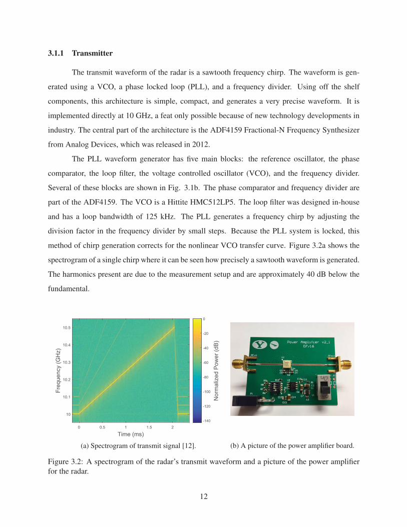
3.1.1 Transmitter

The transmit waveform of the radar is a sawtooth frequency chirp. The waveform is gen-

erated using a VCO, a phase locked loop (PLL), and a frequency divider. Using off the shelf

components, this architecture is simple, compact, and generates a very precise waveform. It is

implemented directly at 10 GHz, a feat only possible because of new technology developments in

industry. The central part of the architecture is the ADF4159 Fractional-N Frequency Synthesizer

from Analog Devices, which was released in 2012.

The PLL waveform generator has five main blocks: the reference oscillator, the phase

comparator, the loop filter, the voltage controlled oscillator (VCO), and the frequency divider.

Several of these blocks are shown in Fig. 3.1b. The phase comparator and frequency divider are

part of the ADF4159. The VCO is a Hittite HMC512LP5. The loop filter was designed in-house

and has a loop bandwidth of 125 kHz. The PLL generates a frequency chirp by adjusting the

division factor in the frequency divider by small steps. Because the PLL system is locked, this

method of chirp generation corrects for the nonlinear VCO transfer curve. Figure 3.2a shows the

spectrogram of a single chirp where it can be seen how precisely a sawtooth waveform is generated.

The harmonics present are due to the measurement setup and are approximately 40 dB below the

fundamental.

(a) Spectrogram of transmit signal [12]. (b) A picture of the power amplifier board.

Figure 3.2: A spectrogram of the radar’s transmit waveform and a picture of the power amplifier

for the radar.

12

The transmit waveform generated by the PLL is amplified using an AMMP-6408 medium

power amplifier chip. The power amplifier is placed on a separate PCB from the PLL as shown

in Fig. 3.2b, which was designed by the author. The AMMP-6408 requires supporting circuitry

to properly bias its transistors. The amplifier is properly biased when its operating current is 650

mA and it is controlled with a negative voltage on the gate of the chip’s transistors. The supporting

circuitry uses a switching regulator to provide a negative voltage source, which is followed with

a voltage division network that allows the gate voltage to be manually changed. When properly

biased, the power amplifier consumes 3.25 W and allows the radar to transmit 25 dBm or 30 mW.

(a) Single Vivaldi antenna, a 1×4 endfire array. (b) Simulated Vivaldi gain patterns at 10.25 GHz

Figure 3.3: Planar Vivaldi antenna used as both the transmit antenna and the receiver antennas for

the radar [12].

Vivaldi antennas from [14] are used as both the transmitting and receiving antennas. They

are designed as end-fire antennas so as to present a low cross section on a flying small-UAS. They

also have a horizontal beamwidth of about 120◦ and a vertical beamwidth of about 30◦. One of

these Vivaldi antennas and a simulated gain pattern are shown in Fig. 3.3.

3.1.2 RF Receiver

The radar features four independent receiver channels. These channels are used in an array

configuration, which allows the radar to back out the bearing of a target, in addition to its range.

13

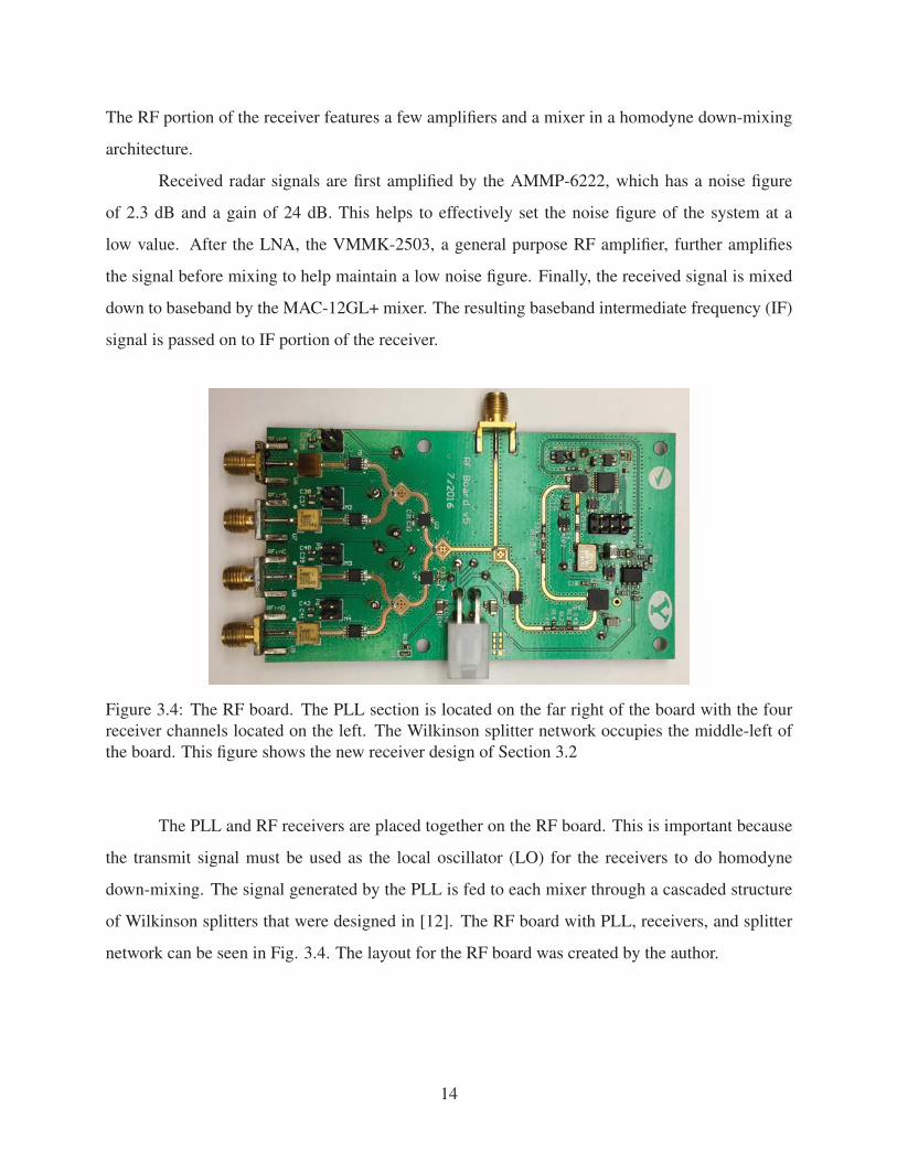
The RF portion of the receiver features a few amplifiers and a mixer in a homodyne down-mixing

architecture.

Received radar signals are first amplified by the AMMP-6222, which has a noise figure

of 2.3 dB and a gain of 24 dB. This helps to effectively set the noise figure of the system at a

low value. After the LNA, the VMMK-2503, a general purpose RF amplifier, further amplifies

the signal before mixing to help maintain a low noise figure. Finally, the received signal is mixed

down to baseband by the MAC-12GL+ mixer. The resulting baseband intermediate frequency (IF)

signal is passed on to IF portion of the receiver.

Figure 3.4: The RF board. The PLL section is located on the far right of the board with the four

receiver channels located on the left. The Wilkinson splitter network occupies the middle-left of

the board. This figure shows the new receiver design of Section 3.2

The PLL and RF receivers are placed together on the RF board. This is important because

the transmit signal must be used as the local oscillator (LO) for the receivers to do homodyne

down-mixing. The signal generated by the PLL is fed to each mixer through a cascaded structure

of Wilkinson splitters that were designed in [12]. The RF board with PLL, receivers, and splitter

network can be seen in Fig. 3.4. The layout for the RF board was created by the author.

14

3.1.3 IF Receiver

The IF subsystem of the receiver takes the IF signal and prepares it for digitization. This

involves amplifying the signal to put it in the range of the ADCs and filtering the signal to reduce

aliasing. The radar’s IF subsystem also uses a range compensation filter to reduce the dynamic

range of the sampled signal. The range compensation filter is combined with amplification in the

first stage of IF subsystem, followed by the second stage which performs more amplification and

anti-alias filtering. The schematic of the IF board can be seen in Fig. 3.5. The PCB of the IF board

was designed to be the same size as the RF board so that they could stack on top of each other. The

size choice for each board was driven by the size of the processing platform, which is described in

Chapter 4. A completed IF board can be seen in Fig. 3.6.

.47uF

C8

2k

R2

2k

R1

2kR8

10R10

.47uFC10

51R7 232

R5

2670

R6

100R11

820R9

200pFC7

200pF

C1

.1uFC11

1kR3

10uFC2

1kR4

In

Out

VCC

-

+Out

V+

V-

U2

LMP7717

VCC

.1uF

C5

1uF

C6

.1uF

C3

1uF

C4

-

+Out

V+!EN

V-

U1

ADA4895

Vsupply

VCC

Figure 3.5: IF Circuit schematic of a single channel [12]

The first two stages are implemented using the ADA4895: a high-gain, low-noise op-amp.

Noise is still a concern at this point because the mixer and 50 Ω matching resistor are lossy com-

ponents. The noise added by this first stage is reduced by the use of a low-noise op-amp and by

careful selection of its surrounding resistors. The stability of this first stage is also a concern be-

cause high gain and parasitic capacitance can lead to oscillations. The parasitic capacitance was

reduced by making a square hole in the copper plane on the bottom side of the IF board underneath

15

Figure 3.6: The IF board. The design of each channel is identical.

the inverting pin of the op-amp. The size of the pad of the inverting pin of the op-amp was also

reduced to mitigate parasitic capacitance. The final design is stable over the entire IF bandwidth.

The range compensation filter is a high-pass filter with a special gain profile. It is evident

from Eq. 2.4 that the received power from a target attenuates by 40 dB per decade as the range

increases due to the 1/r4 relationship. The range compensation filter is a high-pass filter that adds

40 dB of gain per decade which equalizes the attenuation effect due to range. This filter has the

benefit of attenuating strong returns from very close targets and amplifying the returns from far

targets. This also decreases the dynamic range of the signal that will be sampled by the ADCs.

The design of a range compensation filter can only approximate the 40 dB/decade slope.

It is difficult to design a straight 40 dB/decade slope over the entire bandwidth. Additionally, an

ideal anti-aliasing filter response would have a brick-wall at 1 MHz. This would cause issues with

stability and so a filter corner of 50 kHz is used to create a flat response region for the filter.

The last stage of the IF subsystem is the anti-aliasing filter. It is realized using the Sallen-

Key filter topology and is a two-pole low-pass Bessel filter with linear phase response in order to

improve the time domain response. The filter cutoff frequency is 1 MHz, which is half of the 2

Msamp/sec sampling rate. Although it is usually advisable to place the anti-aliasing filter cutoff

slightly lower than half the sample frequency, the natural 40 dB falloff of the radar amplitude due

to range combines with the anti-aliasing filter for an effective falloff of 80 dB/decade. The full

frequency response of the IF subsystem can be seen in Fig. 3.7.

16

Figure 3.7: IF circuit simulated frequency response [12]

3.2 Receiver Dynamic Range Improvement

This section describes an improvement that was made to the radar design. Many minor

changes have been made to the radar design, which included the position of components or indica-

tor LEDs. However, these did not significantly affect the performance of the radar.

One change was made to the receiver design to improve its dynamic range. Because the

radar is a continuous wave radar, the transmitter is always radiating. Because of this, part of the

transmit signal is coupled into the radar’s receivers due to their proximity. The receiver electronics

can then saturate if enough power is coupled into them. This issue is not new for FMCW radars and

is usually considered as a major design constraint for a FMCW system. This constraint means that

the transmit signal power must be limited. This, in turn, limits the detection range of an FMCW

radar.

3.2.1 Design Changes

The RF portion of the previous receiver chain has an LNA, a buffer amplifier, and a mixer

as shown in Fig. 3.8a. The LNA is the AMMP-6222 and has a specified gain of 24 dB with a 1-dB

compression point (P1dB) of 15 dBm. The buffer amplifier is the VMMK-2503, which has 10-dB

of gain and a 10 dB compression point. The mixer is a MAC-12G+ and has a conversion loss of 6

dB and a P1dB of 1 dBm at the input. The mixer is the limiting component in the amount of power

that can be handled by the receiver in this case. That means that the receiver can only tolerate -33

dBm of input power before there is a risk of receiver saturation.

17

LNAAMMP-6222

Buffer AmplifierVMMK-2503

MixerMAC-12GL+CVL = 6 dB

1-dB = 1 dBm

LO

To IF Board

G = 24 dB1-dB = 15 dBm

G = 10 dB1-dB = 10 dBm

(a) Previous RF receiver design

LNAAMMP-6222

MixerHMC412

CVL = 8 dB1-dB = 10 dBm

LO

To IF Board

G = 24 dB1-dB = 15 dBm

(b) New RF receiver design

Figure 3.8: Previous and new receiver chain designs

Based on measurements performed in the lab, an isolation of about 35 dB can be achieved

between the transmitting antenna and the receiving antennas. This means that only -3 dBm can be

emitted by the transmitter to avoid saturating the receivers.

The changes made to the receivers by the author were to remove the buffer amplifier and

use a different mixer. These changes are seen in Fig. 3.8b. The new mixer is an HMC412 and has

a P1dB of 10 dBm at the input and an insertion loss of 8 dB. Using these new figures, the receivers

will not saturate while the transmit power is lower than 16 dBm.

The design change comes with trade-offs of reduced gain and a poorer noise figure. These

trade-offs are overshadowed by the improvement in the maximum detection range of the radar,

which is more than doubled in going from the previous to the new design. This improvement,

along with the associated trade-offs, are detailed in Tab. 3.2. The maximum detection range Rmax

18

Table 3.2: Calculated Results of Design Changes

Receiver Spec. Gsys (dB) P1dB (dBm) Fsys (dB) Rmax (m) PSD (dBm/Hz)

Previous Design 90 1 2.7 158 -81.3

New Design 81 10 4.7 420 -88.3

was calculated with Eq. 2.8 using the appropriate radar specifications and assuming a target of 0.1

m2 and a detection SNR of 15 dB.

There is one caveat to this improvement. The reduced Gsys in the new design may not

provide enough gain to put the noise floor of the radar in the range of the ADCs. This may present

a problem for detecting distant targets because the SNR will be reduced. However, if the noise

floor is in the range of the ADCs, then the new design will realize all the improvements in Rmax.

The PSD’s for both the new and old design are also given for reference in Tab. 3.2.

3.2.2 Measured Design Performance

The new design was tested to measure its performance and the results are summarized in

Tab. 3.3 and 3.4. The radar’s four channels had different values for the receiver specifications. The

results in Tab. 3.3 show the average of the measurements over the four channels. The spread of

the measurements is also shown, where the spread is the difference between the highest and lowest

measurement. The results show that the measured gain is below the calculated gain for the system.

The apparent loss in gain comes from the transition from the RF board to the IF board. The RF

board uses components matched to 50 Ω, while the IF board uses op-amps which have a high input

impedance and a low output impedance. A matching resistor must be placed on the input of the

first op-amp stage to match the RF and IF circuitry. Doing this results in 6 dB of gain loss [12].

Adding 6 dB back into the measured result makes Gsys higher than the calculated value.

The saturation performance of the new receiver design was also tested against the previous

design. This test was done by placing the transmitting and receiving antennas in a plastic frame

as seen in Fig. 3.1a. The frame spaced the receiving antennas 1.5 cm apart with the transmitting

antenna 4.5 cm away from the closet receiving antenna, which was associated with channel A on

19

Table 3.3: Measured Receiver Specifications

Receiver Spec. Gsys (dB) Fsys (dB)

Average Value 77.9 7.5

Spread 1.8 1.8

the radar. This configuration gave an average isolation of 35 dB between the transmitting and

receiving antennas.

The radar was then programmed to transmit a single frequency, while a second signal was

transmitted by an external source and received by the radar. This resulted in a single IF frequency

test signal which was used to monitor the effects of different transmit powers on the receivers. The

results of the comparison are summarized in Tab. 3.4. The new design did outperform the previous

one as it was able to tolerate transmit powers of 18 and 25 dBm without any noticeable loss in the

received signal power.

Table 3.4: Measured Receiver Saturation Performance

Transmit Power 14 dBm 18 dBm 25 dBm

Previous Design No loss 18 dB loss on channel A 18 dB loss on channel A and D

New Design No loss No loss No loss

Both the new and previous design exceeded expectations in the amount of transmit power

that could be tolerated without degradation in the receiver performance. This result indicates that

a mixer may behave differently than an amplifier while saturated. A small signal that goes through

a saturated mixer (which would be saturated by a large signal at a different frequency) may not

experience a significant increase in conversion loss. However, a small signal going through a

saturated amplifier may experience a significant degradation in gain.

20

3.3 Summary

The design of the radar is able to meet the low SWaP requirements of small-UAS by em-

ploying the simple architecture inherent in FMCW homodyne radars to reduce the number, size,

and weight of components needed for an operational radar. Despite the restrictions imposed by a

low SWaP design, the radar is able to provide good sensing capabilities through recent commercial

hardware innovations and a few innovative design choices. The use of a PLL allows the radar to

generate a precise transmit signal which allows a high level of range resolution. A new receiver

design enables the receivers to tolerate power from the transmitter and permits a higher transmit

power to be used. Finally, a unique range compensation IF filter reduces the dynamic range of the

signals sampled by the ADCs.

21

CHAPTER 4. FMCW RADAR SIGNAL PROCESSING ON A LOW SWAP PLATFORM

Digital signal processing is commonly used in modern radar systems. Signal processing

turns raw signals from the radar into meaningful metrics of radar targets such as the range, pointing

angle, Doppler shift, and brightness.

Signal processing is the last major step for this radar system. The main goal of processing

is to produce range and pointing angle information of aircraft around the radar in real time, which

may then be fed to other algorithms for performing collision avoidance. This is a challenge for

small phased array radars, because a digitally steered phased array requires intensive processing

capability. The processing capability for the radar is satisfied using a sophisticated FPGA circuit

as described in [15].

The author’s contribution in the radar’s signal processing was the development of an auto-

matic target detection algorithm and a C++ implementation of the signal processing code which

is run on the ARM processor of the Microzed. This chapter provides a description of the signal

processing steps done in the radar along with a the development of the automatic target detection

algorithm.

4.1 Signal Processing Overview

Signal processing for the radar begins with sampling the output of the radar IF subsystem.

Several things are done with the sampled signals as shown in Fig. 4.1. The final output of the

current DSP system are range and angle pairs of potential targets in the field of view of the radar.

The signal processing steps are (1) sampling the voltages from the IF circuit, (2) transform-

ing the time-domain signals to the frequency domain via the FFT, (3) correlating the data from each

of the channels, (4) averaging the correlated data, (5) performing automatic target detection on the

correlated and averaged data, and (6) determining the angle of arrival (AOA) of detected targets

through digital beamforming. Additional processes can be added after this point such as target

22

ADCs

FFT

Correlation

Averaging

Target Detection

Beamforming

Target Tracking

Collision Risk Assessment

Avoidance Path Planning

BOARAC Interface Board

MicroZedFPGA

MicroZed ARM Processor

Yet to be integrated

Figure 4.1: Block diagram of the DSP system.

tracking, collision risk assessment, and avoidance path planning. These final steps have not yet

been integrated into the radar system.

4.1.1 Signal Processing Platform

The digital processing platform of the radar comprises two boards: the MicroZed and the

BOARAC board. These boards can be seen in Fig. 4.2. The MicroZed is a comercially available

board which has a Zynq 7000 chip. The Zynq 7000 is a hybrid chip that has an FPGA fabric and

two ARM A9 processors integrated together. A light version of Linux called Wumbo is run on the

processors which facilitates the processing flexibility of the MicroZed. The MicroZed provides all

the required computing for the radar through digital circuits on the FPGA and the flexibility of its

CPUs.

The BOARAC board is a custom carrier board for the MicroZed. It was designed by

Newmeyer and Wilde in [15] through the Center for High-Performance Reconfigurable Comput-

ing (CHREC). The BOARAC board has 8 ADCs that can sample at 2 Msps. Only 4 ADCs are

23

Figure 4.2: The MicroZed (left) and BOARAC (right) boards. The MicroZed houses the FPGA

and processor for signal processing while ADCs are located on the BOARAC board which perform

the sampling [12].

used in the radar system and the data from these ADCs are sent through the BOARAC board to the

MicroZed for processing.

The following sections will detail the processing steps which the radar follows. All the steps

outlined below are implemented through the FPGA on the MicroZed or in C++ on the MicroZed’s

processors. Increased emphasis will be placed on the automatic target detection algorithm, as this

was the main contribution of the author to the radar’s digital signal processing.

4.2 Signal Digitization and Fourier Transform

Despite being a CW system, the signals from the radar are sampled in blocks of time that

are synchronized with each radar pulse. This avoids sampling ambiguous IF signals that occur at

the start and end of each frequency chirp of the transmitter as shown in Fig. 4.3. This sampling

scheme enforces the relationship

NFFT = Tc fs, (4.1)

where NFFT is the number of samples in a single sampling block, Tc is the chirp period, and fs

is the sampling frequency. The subscript notation on NFFT alludes to the fact that the number of

24

Figure 4.3: Illustration of the relationship between the sampling blocks and the transmitted chirp.

The orange and blue line on the frequency axis represent the transmitted and received chirps re-

spectively. The waveform on the amplitude axis represents the IF signal resulting from the received

chirp.

samples in a block will also be the same as the number of samples used in the FFT. The current

system collects NFFT = 4096 samples in each block with Tc = 2.048 ms and fs = 2 Msps. On the

radar hardware, these samples are collected by ADCs located on the BOARAC board and sent into

first-in-first-out (FIFO) buffers on the FPGA fabric of the MicroZed.

After sampling, an optional operation before taking the FFT of the data is to window the

data. The motivation for using a data window comes from the fact that the window affects some

characteristics of the FFT such as scalloping loss and spectral leakage. Scalloping loss occurs

when the frequency of a signal falls between two frequency bins in the FFT. This causes the power

of a signal to be split between two bins which will result in a small loss in SNR. Scalloping loss is

not a concern for the radar, because its range resolution is small enough (0.6 m) that a target will

usually be in multiple frequency bins.

Spectral leakage has two meanings. First, spectral leakage can refer to how the sidelobes

of a window function can allow strong signals at one frequency to leak into different frequencies.

It can also refer to the fact that the DFT and FFT rely on the assumption that the signal in its

25

sampling window is periodic with the sample window. That is, if one sampling window was put

side by side with infinite copies of itself, the result would be a continuous signal of one frequency.

Spectral leakage is a concern for the radar because (1) strong signals exist which could leak into

nearby frequencies because of the sidelobes of a window function and (2) because the signals in a

sampling block will often not be periodic with themselves. However, this was not fully considered

in the original hardware design and so a rectangular window is used by default.

The next processing step is to estimate the frequencies in the sampled data which corre-

spond to the ranges of different radar targets. This is done by transforming the sampled data to the

frequency domain via the DFT implemented with an FFT. The radar uses NFFT sample points in

the FFT, which is a power of two to allow a fast execution of the FFT. Of the 4096 output samples

of the FFT, only the first 2048 samples corresponding to positive frequencies are kept for further

processing. The radar hardware implements the FFT on the FPGA fabric on the MicroZed.

In order for the radar to operate in real time, it must perform the 4096-point FFTs on each

of the four channels every 2 ms. This results in a computation requirement of approximately 144

MFLOPs. The implemented FPGA design completes this task in 1.2 ms [15].

4.3 Correlation and Averaging

The next step after sampling and transforming the sampled data is correlating the data from

each antenna element and then averaging over consecutive radar pulses. Correlation is an operation

that allows phased array processing over array elements.

The data collected from the radar can be organized into a data cube as shown in Fig. 4.4.

The frequency bins can be indexed by i, each pulse by m, and each channel by A, B, C, or D.

Correlation uses the data vectors

xi[m] =[Ai[m] Bi[m] Ci[m] Di[m]

]T, (4.2)

to form a correlation matrix for each pulse and frequency index. The correlation matrix R is formed

from the outer product of xi[m] as

Ri[m] = xi[m]xi[m]H . (4.3)

26

Cha

nnel

A

B

C

D

Pulse Index

Figure 4.4: Radar data organized into a data cube. The frequency bins of each FFT, or the fast-

time data, are indexed with i. Each pulse, or slow-time index, is indexed with m. Each channel, or

spatial index, is referred to as channel A, B, C, or D. The column highlighted in green illustrates

the data used to create a correlation matrix for one pulse and frequency bin.

The averaging step in correlation combines correlation matrices from multiple pulses to create

an averaged correlation matrix Ri. This part of correlation reduces the data rate of the radar.

The correlation and averaging operations are implemented in hardware in a slightly modified way.

Because Ri is Hermitian, only the correlation of elements of the upper triangle are computed. Thus,

for 2048 frequency bins every 2.05 ms, correlation requires 60 MFLOPs.

Four FFTs are done in parallel for each channel on the FPGA. The output is directly piped

into the FPGA hardware that performs correlation without requiring staging memory. The output

of the correlator is then piped directly into the averager which computes the average of several

pulses using a running sum. The number of averages can be selected by powers of 2 ranging from

1 to 64 pulses.

4.4 Automatic Target Detection

Automatic target detection is an important step in processing radar signals. Modern radars

use automatic target detection to filter out returns due to noise or clutter and report only targets

27

of interest. This helps save computer and operator resources. Automatic detection is especially

important for the radar so that it can identify potential targets.

Ideally, the radar would attempt detection after beamforming when a target’s SNR will be

at its maximum. This is not done because of the large set of data that needs to be manipulated by

beamforming to produce an image of the radar’s entire field of view. Target detection is used at

this stage to select range bins where targets were detected. Then, beamforming is only done on

those range bins. Unlike the FFT and correlation steps, the detection algorithm runs on the system

processor of the MicroZed rather than the FPGA hardware. In fact, all of the steps following

correlation and averaging are done on the system processor.

A straightforward approach to automatic detection is to set a uniform threshold, that does

not vary by range or angle, which determines whether or not a return is classified as a target. A

return is a target when its amplitude rises above the threshold. Otherwise the return is ignored.

Usually this threshold is set above the noise in a radar system to achieve some probability of false

alarm or PFA. A uniform threshold approach does not work for the radar because the radar scene

(i.e. a snapshot of return amplitude vs. range) is not homogeneous. The scene will have legitimate

clutter returns from hills, trees, and buildings that may make it above the threshold, but are not

targets of interest to the radar. The radar scene will also be changing as a host UAS changes

position. A more flexible threshold is needed that ignores some clutter and also changes over time

to reflect change in the radar scene due to movement.

Special detection methods called constant false alarm rate (CFAR) algorithms exist that

compute an adaptive threshold to identify targets in radar data. An ordered statistic CFAR (OS-

CFAR) algorithm was implemented to perform automatic target detection on the BYU radar. This

particular CFAR method was chosen because it provides robust performance when multiple targets

are present and possibly adjacent to each other. It does come at the cost of increased computation

time and higher SNR requirements. The following section describes the design of this algorithm.

28

4.4.1 OS-CFAR

OS-CFAR Overview

The OS-CFAR sets a threshold value for each range bin in the range compressed image

(RCI) based on two parameters: (1) the estimated noise power for each range bin and (2) the

desired PFA. The threshold value T for one bin can be calculated using

T = α g, (4.4)

where g is the noise power estimate and α is a scaling value related to PFA.

The algorithm estimates the noise power in each range bin based on its neighboring range

bins. The neighboring bins are referred to collectively as the CFAR window as seen in Fig. 4.5

and the number of bins in the window, or the window length, is denoted with N. The OS-CFAR

algorithm sorts the return powers of the N range bins in the CFAR window and selects the Kth

smallest return power as the noise estimate for the cell under test (CUT). It then slides the window

along, computing the noise estimate for the next CUT.

Figure 4.5: Diagram of a CFAR’s sliding window.

The constant α is determined by PFA, the window length N, and the statistical properties

of the noise. It raises the threshold far enough above the noise in a range bin to achieve the

desired PFA. How high the threshold needs to be raised above the noise level is determined by the

underlying statistics of the noise in the radar system.

29

Assuming the noise input into the radar is additive white Gaussian noise for the simple case

where there are no targets (i.e. when the radar is pointed at a cool sky), the noise statistics at the

threshold detection step can be derived as follows.

Distribution of the DFT of a White Gaussian Process

We begin with a sequence of random variables (r.v.) xn with n = 0, 1, 2, . . ., N −1 that are

independent and identically distributed Gaussian r.v.’s with zero mean and common variance σ2

and which we denote the PDF of with Gσ . To derive the statistics we will use Eqs. 2.9, 2.10, and

2.11.

To begin, the sequence xn represents data samples from the ADCs. The N−1 long sequence

is transformed into the frequency domain through the DFT (implemented via the FFT) as

Yk =1

N

N−1

∑n=0

xne j 2πnkN . (4.5)

By first considering the real part we get

R{Yk}= 1

N

N−1

∑n=0

xn cos

(2πnk

N

), (4.6)

where it can be seen that for each n and k, the cosine term is simply a scaling factor which we

denote cn,k. Thus, using Eq. 2.9, the PDF of the nth term in the summation is

1

cn,kGσ

( xcn,k

), (4.7)

which is another Gaussian r.v. with variance σ2n,k = σ2c2

n,k. We denote the PDF of this r.v. with

Gn,k.

This leaves us with a sum of Gaussian r.v.’s, which is also a Gaussian random variable by

the central limit theorem. We can find the variance of this sum using Eq. 2.10, the characteristic

functions of the r.v.’s, and Eq. 2.11. This results in

N−1

∏n=0

Φn,k =N−1

∏n=0

e jω2σ2n,k . (4.8)

30

The variance σ2k of the sum of the r.v.’s is

σ2k =

N−1

∑n=0

σ2n,k =

N−1

∑n=0

σ2 cos2

(2πnk

N

), (4.9)

which is σ2N for k = 0 and σ2N/2 otherwise. By using Eq. 2.9 again for the 1/N normalization

factor, the real part of the DFT sum for k �= 0 results in a Gaussian r.v. with variance σ2/2N. This

development also applies to the imaginary part of the DFT sum and results in a Gaussian r.v. with

the same variance.

Square Law Detector Distribution

The FFT step in the radar signal processing produces a complex sequence where both the

real and imaginary parts have Gaussian distributions. Now it will be shown that given this input,

the distribution of the correlation output is exponential. Consider the complex, white Gaussian

random variable W = X+ jY, where X and Y are also white Gaussian r.v.’s with zero mean and

common variance σ2. We wish to know the distribution of the r.v. Z = |W|2 = X2 +Y2, which is

produced by correlation.

The cumulative distribution function (CDF) of Z is such that P{Z ≤ z} = {X2 +Y2 ≤ z}.

One can recognize that P{X2+Y2 ≤ z} is a region inside a circle of radius√

z. The CDF of Z can

then be found by integrating the joint PDF of X and Y over this region. Using polar coordinates

and the substitution x = r cos(θ) and y = r sin(θ), this results in the integral

∫ 2π

θ=0

∫ √z

r=0

1

2πσ2e−r2/2σ2

rdrdθ . (4.10)

Evaluating this integral results in

∫ 2π

θ=0

∫ √z

r=0

1

2πσ2e−r2/2σ2

rdrdθ =1

σ2

∫ √z

r=0re−r2/2σ2

dr

=∫ z/2σ2

u=0e−udu

= 1− ez/2σ2, (4.11)

31

where the substitution u = r2/2σ2 was made. By differentiating this result with respect to z, we

obtain the PDF of Z which is

pZ(z) =1

2σ2e−z/2σ2

, z ≥ 0. (4.12)

Thus, the PDF of the magnitude squared of a complex, white Gaussian random variable with

zero mean is an exponential random variable with parameter 1/2σ2. This is an important result

because equations that specify PD and PFA for OS-CFAR detectors assuming an exponential noise

distribution have already been derived.

OS-CFAR Design

Equations may be derived that specify PD and PFA once the noise statistics at the detection

step are known. For a square law detector with exponentially distributed noise power, [13] gives

expressions for both PFA and PD for the OS-CFAR as follows:

PD =K−1

∏i=0

N − iN − i+ α

1+SINR(4.13)

and

PFA =K−1

∏i=0

N − iN − i+α

, (4.14)

where N is the length of the CFAR window, K is the ordered statistic selection, α is the scale factor

in Eq. 4.4, and SINR is the signal-to-interference noise ratio.

Equations 4.13 and 4.14 can be used to generate receiver operating characteristic (ROC)

curves that relate SINR and detection performance. The curves can be used to design an OS-CFAR

and to determine the needed level of SINR performance when given a desired PD. Several ROC

curves have been generated for the OS-CFAR and they can be seen in Fig. 4.6.

As an example, Fig. 4.6a can be used to show that an SINR of 18.5 dB is required to

achieve a PD of 0.8 while maintaining a nominal PFA of 10−5 when using a window length of 32.

Larger values of PFA could instead be chosen to lower the SINR needed to achieve a PD of 0.8, but

this comes at the cost of more false detections. The radar performs one detection test for each of

32

SINR (dB)14 16 18 20 22 24 26 28 30

Prob

abili

ty o

f Det

ectio

n

0.5

0.55

0.6

0.65

0.7

0.75

0.8

0.85

0.9

0.95

1

PFA

= 10-3

PFA

= 10-4

PFA

= 10-5

PFA

= 10-6

(a) ROC curves for four values of PFA while

maintaining N = 32 and K = 24.

SINR (dB)14 16 18 20 22 24 26 28 30

Prob

abili

ty o

f Det

ectio

n

0.5

0.55

0.6

0.65

0.7

0.75

0.8

0.85

0.9

0.95

1

N = 16 N = 32 N = 48 N = 64

(b) ROC curves for four values of N while main-

taining PFA = 10−6. The parameter K is adjusted

for each N according to K = 3N/4�.

Figure 4.6: ROC curves for the OS-CFAR.

the 2048 range bins in each RCI. These RCI’s are gathered at a rate of about 1 RCI every 70 ms.

With a PFA of 10−5, there would be three false alarms per 10 seconds on average. How many false

alarms can be tolerated is dictated by the requirements associated with the tracking algorithms for

the radar.

The curves in Fig. 4.6b show how PD changes for different OS-CFAR window sizes. They

also suggest that a window size of N = 32 yields a good improvement in performance without

being burdened by a large window size (sorting has a computational complexity of O(n logn)).

OS-CFAR Performance

The performance of an OS-CFAR detector for the radar was analyzed in post-processing

using real radar data. The data in this analysis comes from an experiment where the radar was

located on the ground and was imaging a flying X8 multi-copter. The OS-CFAR detector used

operating parameters of N = 32, PFA = 1× 10−3, and k = 24. The larger PFA value was used

because the X8 return was not strong enough to make it into the detection region of a more common

PFA of 1× 10−6. Figure 4.7 shows one RCI of the radar with the CFAR detection threshold. The

return of the X8 can be seen around 100 meters. The return obviously makes it into the detection

region with about 15 dB of SINR compared to the returns close to it. Based on the ROC curve in

33

Range (m)0 20 40 60 80 100 120 140 160 180 200

Pow

er (d

Bm

)

-70

-60

-50

-40

-30

-20

-10

0

Radar RCICalculated Threshold

Figure 4.7: A snapshot of the threshold generated by the OS-CFAR algorithm over range. The

return of a flying X8 multi-copter can be seen near 100 m.

Fig. 4.6a, this puts the PD of the X8 near 0.8. The other returns near the X8’s return come from

clutter objects in the radar’s environment.

The performance of the CFAR detector over time can be seen by applying it to multiple

RCI’s of the radar. The images in Fig. 4.8 show range verses time maps of the radar data gathered

while imaging the X8 multi-rotor. The image of Fig. 4.8a shows the power of the X8 returns as

the X8 flies away from the radar. Additional returns from clutter in the environment can also be

seen in the vicinity of 75, 100, 100, and 115 m. The clutter returns around 75 m pose a detection

problem because they compete with the X8 returns.

Figure 4.8 shows the result of applying the CFAR detector to each of the RCI’s from the

radar. The track of the X8 can be seen as a black slanting line where the CFAR detector declared

a detection. More of the X8’s returns made it above the detection threshold at two seconds than

at half a second, even though the power of both returns are about equal. This is because the

clutter returns around 75 m reduced the SINR of the X8. The clutter returns essentially counted

as additional interfering targets in the CFAR’s window. OS-CFAR’s are designed to be robust to

multiple interfering targets. The number of targets they can be robust to is N − k, which in this

case is 8.

34

Time (s)0 1 2 3 4 5

Ran

ge (m

)

70

75

80

85

90

95

100

105

110

115

120

-50

-45

-40

-35

-30

-25

-20

-15

-10

-5

(a) A range vs. time intensity map of radar data

while imaging a flying X8 multi-copter. Color

scale values are in dBm.

Time (s)0 1 2 3 4 5

Ran

ge (m

)

70

75

80

85

90

95

100

105

110

115

120

(b) A range vs. time map of radar data that has

had the OS-CFAR threshold applied to it. Black

marks represent returns identified as targets.

Figure 4.8: Range vs. time maps of radar data while imaging a flying X8 multi-copter.

4.5 Clustering

Applying the threshold generated by the OS-CFAR algorithm to the radar’s RCI data often

results in groups of adjacent range bins where targets were detected. These groups are called

clusters. An example of this is the cluster generated by the X8 in Fig. 4.8 where the slanting

line grows thicker. These clusters always have a few range bins were the echo power is much

stronger than the echos from range bins in the same cluster. The clustering algorithm selects one

of these range bins to represent each cluster of targets in order to further filter the data passed to

beamforming.

Two options exist for which bin to select as a cluster’s center. A weighted averaged or

centroid could be used to represent the cluster. This makes sense intuitively because it places the

center of the target at its brightest or biggest area. The centroid will be a non-integer range bin and

must be rounded to an integer because beamforming can only be done on integer range bins. One

concern with using a centroid to represent the cluster is that while the centroid will be very close

to the bin with the highest return power, the rounded centroid may be a bin where the SNR is low.

This may reduce the accuracy of estimating the AOA in beamforming.

The range bin with the highest power could also be chosen to represent a cluster. This

choice does not make as much sense intuitively. However, it does maximize the SNR for the

35

beamforming step. It is for this reason that clustering was implemented by choosing the range bin

with the highest return power as the center of a cluster.

4.6 Beamforming

Digital beamforming allows the radar to determine the AOA of echoes. Beamforming is

very similar to electronically scanned arrays in that it adjusts the phase of the signal at each antenna

to steer the look direction of a phased array. The main difference is that digital beamforming is

done digitally rather than in analog hardware.

Steering the receiver array of the radar produces a narrower beam than the Vivaldi antennas

have by themselves. The 3-dB beam width of the steered beam varies between 25.5◦

for steering

at bore sight and 32◦

for steering 30◦

off of bore sight. The gain of the array also varies between

18-dB and 16-dB for the same steering angles [14].

The AOA of a target in one range bin is found by computing the received power for Nbeams

steering angles that cover the antennas’ field of view, which is typically +45◦/-45◦. The steering

angle with the highest power is then selected as the AOA for that range bin. This method makes

the assumption that there is only one target in each range bin.

An approximate weight vector w for each steering angle can be formed by

w =[e jk·rA e jk·rB e jk·rC e jk·rD

]T, (4.15)

where rA, rB, rC, and rD are the position vectors of each of the antenna elements. The k term in

Equ. 4.15 can be expanded as k = k · r where k is the wave vector and r is a unit vector pointing

in the desired steering direction. This is an approximate weight vector because the array will have

variations in phase and gain that should be accounted for through calibration.

The power S(i,a) received at the ath steering angle, of the Nbeams steering angles, at the ith

range bin can be computed using the corresponding weight vector wa and the averaged correlation

matrix Ri. This is done by

S(i,a) = wHa Riwa. (4.16)

36

This computation is only performed for the range bins left after clustering. After the angle

with the highest power is determined, the radar processing has produced an estimate for the range

and AOA of a target.

Beamforming is the last step in the DSP chain that has been successfully integrated into

the radar system. There are three additional steps that can possibly be done on the MicroZed

processor to extend the capability of the radar system. These steps are briefly described in the

following section.

4.7 Tracking and Collision Avoidance Processing

The digital processing steps just described have all been successfully integrated together

into the radar system. Together, they produce range and angle estimates for targets in the radar’s

field of view.

These estimates are the main product of the radar as a collision avoidance sensor. The

information is only valuable, though, if it can be used to direct a small-UAS out of a collision

scenario. This capability involves tracking targets detected by the radar, determining if a collision

encounter is possible, and then planning an avoidance path to minimize the risk of a collision as

indicated in Fig. 4.1.

Beyond the radar’s scope, extensive work has been done on implementing these steps. The

recursive RANSAC (R-RANSAC) tracking algorithm developed by Niedfeldt, et al. in [16] is a

multiple target tracking (MTT) algorithm that performs well in the presence of clutter. Work on

collision risk assessment and avoidance planning has been done by Sahawneh, et al. in [17] and

[18] using a probabilistic risk estimation model and chain-based path planning. These algorithms,

or similar ones, could be integrated with the radar to create a full collision avoidance system for

small-UAS.

4.8 Summary

The signal processing capabilities of the radar enhance its abilities as a sensor. Because of

the operation of an FMCW radar, taking the FFT of the radar signal effectively applies a matched

filter bank to the received signal which spreads out the noise power across all frequency bins and

37

maximizes the SNR of the radar. Data intensive tasks like the FFT and correlation can be performed

in real time by a custom FPGA digital circuit design. The radar also uses an automatic target

detection algorithm to identify and budget processing resources to targets of interest. The angle of

arrival of these target can then be determined through DBF where the radar simultaneously scans

multiple angles in its field of view to determine the angle with the highest return power. Finally,

collision avoidance algorithms could be integrated with the radar system to make it a full sense and

avoid system for small-UAS.

38

CHAPTER 5. A SIMULATION MODEL FOR A LOW SWAP FMCW RADAR

System models help in the design process because they allow the design to be tested without

requiring a hardware prototype to characterize the design. An FMCW radar simulation model was

created to set performance expectations for the SNR, maximum range, and other specifications

of the radar. The model was also developed to simulate encounter scenarios and develop signal

processing code for the radar. This chapter discusses components relating to the development of

the radar model as well as the radar simulation model itself.

5.1 Noise and Signal Power

It is important for a radar simulation model to accurately estimate the signal received by

a radar. Two signal characteristics to estimate are the power levels of the received signal and the

noise. The power of a signal Prec received by the radar is modeled using Eq. 2.4 and then multiplied

by the IF gain GIF. This power is then converted to RMS voltage amplitudes using Vrec =√

PrecR

where R = 50 Ω. The noise power in the system is calculated using Eq. 2.5 and multiplying again

by GIF. The RMS noise voltage Vn can then be calculated using Vn =√

N0R, where again R= 50 Ω.

The theoretical SNR of the radar system can then be calculated for different targets using

these noise and signal equations.

5.1.1 Worked Example

A worked calculation of SNR is presented here to illustrate what SNR is expected from the

radar. The specifications of the radar are used in the example.

Problem

If the radar viewed a 12 in diameter aluminum sphere 39 m away, what is the output power of

the signal, noise, and what is the SNR? The transmitted power is 12.5 dBm, the transmitter and

39

receiver antenna gains are 12 dB, the receiver power gain is 92 dB with a noise figure of 3.14

dB, and the radar’s operational wavelength is 3 cm. For an FMCW radar, the receiver bandwidth

is determined by the bandwidth of an FFT bin. The value for this is 490 Hz for the radar. Also

assume the background temperature and antenna are at 290 K.

Solution

First change decibels to linear units: 12.5 dBm = 17.7 mW, 12 dB = 15.85, 92 dB = 1.58× 109,

3.14 dB = 2.06, and the RCS for a metal sphere is πr2 which in this case is 0.071 m2. Using Eq.

2.4, the received power is

Prec =(0.0177)(15.85)2(0.03)2(0.071)

(4π)3(39)4(1.58×109) = 98 μW =−10.1 dBm. (5.1)

The noise power is given by Eq. 2.5. The receiver equivalent temperature Te can be related

to noise figure by Te = (F −1)T0, where T0 is 290 K. Using this, the output noise power is

N0 = (1.38×10−23)(290+307.4)(490)(1.58×109) = 6.38 nW =−51.95 dBm. (5.2)

Comparing the signal power to the noise power yields an SNR of 41.85 dB. It will be

seen that the radar system performs very close to this SNR value in the calibration testing done in

Chapter 6.

5.2 Maximum Detection Range and RCS

Successful UAS collision avoidance requires that the intruding aircraft is detected in time

so that the UAS can perform an avoidance maneuver. This requirement translates to a minimum

detection range for successful collision avoidance.

Sahawneh in [4] shows that the minimum detection range is partly determined by the clos-

ing speed of an encounter. He also explains that smaller aircraft generally move slower while

heavier and larger aircraft move faster. Sahawneh’s calculations indicate that a minimum detection

40

range of about 800 meters is needed for a head-on collision encounter of two small UAS where the

closing speed is around 60 m/s. The minimum detection range for successful collision avoidance

puts a constraint on the detection range of a SAA radar sensor. The maximum range of the radar

must be greater than or equal to the minimum detection range.

The maximum range depends on several factors. Two of these factors are the radar cross

section (RCS) of the target and the power of the transmitted pulse. The transmit power is limited

by the low SWaP constraints of small-UAS. The RCS of small-UAS are also small because they

are often constructed from non-metallic materials. The limited transmit power and small RCS can

thus limit the maximum range of the radar.

With these considerations in mind, a plot of the maximum range of the radar verses RCS

was created to help characterize the capabilities of the radar system. The maximum range was

calculated using Eq. 2.8, where only the transmit power and RCS were changed. The values for

the other radar specifications that remained fixed are given in Tab. 5.1. The resulting plot is shown

in Fig. 5.1 where several range verses RCS curves are shown for different transmit powers Pt .

Table 5.1: Radar Specifications for Calculating the Maximum Range

Parameter ValueGt 12 dB

Gr 18 dB

λ 3 cm

SNR 15 dB

T 290 K

F 5 dB

B 1 kHz

The plot of Fig. 5.1 takes on practical meaning when the RCS of a typical small-UAS

is considered. It is difficult to determine the RCS of a small-UAS analytically because the RCS

depends on the operating frequency of the radar, the incidence angle, and characteristics of the

small-UAS such as its material, its shape, and its size. Some useful RCS measurements of a

30× 30× 20 cm2 quad-rotor UAS were obtain by Tsai, et al. in [19]. They measured the RCS

of the UAS from a few incident angles and found that the RCS varied between -15 dBsm and -5

41

dBsm (or about 3.2 cm2 to 32 cm2) at X-band. For reference, the RCS of a human is around 1 m2

at X-band.

Radar Cross Section (m2).01 .1 1 10

Det

ectio

n R

ange

(m)

0

250

500

750

1000

1250

1500

1750

2000

Pt = 1 mW

Pt = 100 mW

Pt = 1 W

Pt = 2 W

Pt = 4 W

Figure 5.1: Plot of Rmax verses RCS

By referencing Fig. 5.1, it can be seen that at least 4 W of transmit power is needed to

detect the small-UAS in [19] from 800 m in the worst case scenario where the RCS is 3.2 cm2.

In the best case scenario where the RCS is 32 cm2, less than 1 W of transmit power is required

to detect the UAS at 800 m. Because the RCS measured in [19] varies by incident angle, this

shows that there is large variation in the RCS of a small-UAS depending on it its orientation with

respect to the radar. Currently, the radar operates with a typical transmit power of 800 mW, which

is sufficient to detect a small-UAS with an RCS no smaller than 20 cm2.

5.3 1D Phased Array Radar Model

A simulation model of the radar was created to help develop processing code and to perform

simulations of encounter scenarios between an ownship and an intruder aircraft. The model is

referred to as the 1D phased array radar model because it simulates the radar signals received

42

by a one-dimensional antenna array. This model incorporates the equations used in section 5.1

to calculate the received signal power and noise power in the radar. It also includes other sub-

components, which are described later, in order to create the entire simulation model.

A high-level diagram of the simulation model can be seen in Fig. 5.2. The analog script,

post-processing, and simulation update blocks run in a loop within the main script. The analog

script utilizes the equations in section 5.1 and the other sub-models to synthesize the raw radar

signals received by the antenna array. The post-processing block processes, saves, or plots the syn-

thesized data. Most often, the post-processing block is the processing scheme outlined in Chapter

4. Finally, the update simulation block updates the parameters of the simulation such as target

locations and the radar’s orientation.

Main Script

Analog Script Post-Processing

Update Simulation

Figure 5.2: High-level block diagram of the 1D phased array radar model.

The analog script models the voltages sampled by the ADCs, the antenna’s field of view,

the phase difference between antennas due to signal propagation, and thermal noise. It can also

account for the position of a target in three-dimensional space and the radar’s own position and

attitude. The script uses several simplifying approximations. It uses simple hard targets which are

represented by points in space with a constant RCS value. This is not entirely accurate as the RCS

of most real targets fluctuate. The noise received by each antenna is also approximated as isotropic

noise, that is, the noise in one channel is independent of the noise in another channel. This is not

quite accurate for a physical system because of coupling between antennas. The model can also

also incorporate general hardware losses. The phase noise generated by the VCO is not accounted

for. The following sections describe the sub-models used by the radar simulation model.

43

5.3.1 Antenna Model

The simulation model uses a rectangular aperture antenna to simulate the FOV of the radar.

Although this does not model the exact antenna pattern of the Vivaldi antennas in Fig. 3.3, it does

give a simple way to define the beamwidth of the antennas such that the beamwidth of the Vivaldi

and simulation antennas are the same.

The antenna pattern of a rectangular aperture antenna with a uniform current distribution is

well studied and [20] gives the antenna pattern as

F(φ) = sinc2(πlysin(φ/λ )), (5.3)

where φ is the angle off boresight of the antenna in the y-z or azimuth plane, ly is the size of the

width of the aperture in the horizontal or y-direction, and λ is the wavelength.

The antenna model is incorporated into the simulation by multiplying Eq. 2.4 by the square

of Eq. 5.3 and also by Eq. 5.3 squared again, instead replacing φ with θ (the angle in the x-z or

zenith plane) and ly with lz (the size of aperture in the vertical direction).

5.3.2 Phased Array Propagation Model

The phase difference of the received signal at each antenna is an important feature for the

analog script to model. The phase differences are used by the DSP code to derive an AOA from

real radar data.

The propagation model assumes that the target is far away so that the incident wave from

a target on the antenna array is a plane wave. Figure 5.3 shows the physical layout of a typical

scenario for such a phased array. Because the incident wave is approximated by a plane wave, the

phase difference between antenna elements is not dependent on the distance between the target and

each element. Rather, it is dependent on the AOA and the relative position of the elements which

includes the spacing d for a uniformly spaced array.

The phase difference between each element is Δφ = ωΔt, where Δt is the arrival time

difference between elements and ω is the angular frequency of the wave. The time difference is

Δt = Δd/c where Δd is the relative spacing of the elements with respect to the source and c is the

speed of light.

44

d

θ

Target

Figure 5.3: Phased array diagram for an array with elements i = 0,1,2,3.

As can be seen in Fig. 5.3, the distance Δdi between the element at the origin and the

element at position i is given by projecting the position vector of the antenna element ri onto a unit

vector directed towards the source or target. This projection will give Δdi for a 1D or 2D phased

array. Then, the relative phase of element i to the element at the origin is

Δφi =ωΔd

c. (5.4)

A vector of the phase differences between each antenna can then be found by ΔΦ = k(r · ri). The

phase differences these give can then be added to the signal at each antenna element to simulate

the operation of a phased array system.

5.4 Summary

Creating a simulation model for the radar is valuable because it can be used to modify and

refine the hardware design of the radar. The equations which describe the simulation model for the

radar can also be used to estimate the maximum range of the radar based on current design speci-

fications. The simulation model accounts for free space path loss, electronics noise, antenna field

of view, and phase differences between multiple antennas due to their placement. The simulation

model is also useful for developing the signal processing code for the radar.

45

CHAPTER 6. EXPERIMENTAL RESULTS

The previous chapters have described the hardware design, signal processing, and simu-

lation model for the FMCW radar. An important aspect of the radar’s development is testing its

capability in the field. There are two significant tests for the radar which demonstrated its capa-

bilities. The first type of test was used to verify the radar’s SNR performance and to check the

accuracy of the radar simulation model. The second test which was performed allowed the radar

to operate on board a small-UAS with the goal of detecting other small-UAS. Both of these tests

are described in the following sections.

6.1 Radar Calibration

Calibration tests are used to measure the field performance of the radar. They help deter-

mine the operating SNR of the radar and identify needed improvements in the design. Calibration

tests have been performed throughout the radar’s development [12].

These tests have been augmented by comparing the test results with simulations produced

by the radar model described in section 5.3. This comparison allows the accuracy of the simulation

model to be quantified. Deviations of the model from test results can be used to correct the model

or debug the hardware.

The calibration test was done in the west parking lot of the BYU stadium. This location

was chosen because the asphalt backscatter was small and it was free of clutter objects (cars, light

poles, fences, houses, trees, etc.) for about 80 m in the direction of the radar beam.

6.1.1 Calibration Experimental Results and Model Comparison

The calibration test used a metal sphere with a diameter of 12 in as the radar calibration

target. The sphere was placed on a 5 ft cardboard pole to raise it away from the ground. The radar

was set up on a 3 ft table with its boresight pointed at the sphere. The distance between the sphere

46

and the radar was set at 39 m. A personnel member also stood near the sphere as a reference target,

but was at a different range by several meters.

The plots in Fig. 6.1 display range compressed image (RCI) data generated by the radar

and the radar simulation model which is zoomed in on the sphere target. The blue curves are the

radar data while the red curves are from simulation. The sphere is located at about 40 m in each

of the figures. The curves in Fig. 6.1a are plotted from a single RCI. Figure 6.1b plots 1000 RCIs

that have been averaged together. The signature of the personnel member is clearly seen at about

33 m in Fig. 6.1b of the averaged RCIs.

Range (m)0 10 20 30 40 50 60

Pow

er (d

Bm

)

-70

-60

-50

-40

-30

-20

-10

Radar DataSimulation Data

(a) One RCI of radar and simulated data.

Range (m)0 10 20 30 40 50 60

Pow

er (d

Bm

)

-60

-50

-40

-30

-20

-10

Averaged Radar DataAveraged Simulation Data

(b) Plots of 1000 averaged RCIs from the radar

and simulation data.

Figure 6.1: RCI plots of the stadium parking lot test zoomed in on the sphere, which is located at

about 40 m.

The signal power of the radar model is about 5 dB stronger than the real radar data. This

shows that the simulation model is accurate to a factor of about four. The discrepancy could be

due to unseen losses in the radar, incorrect values used in the model for Gt , Gr, or multipath in the

test environment. The RCS, range, and Pt are not likely the cause because they can be measured

accurately. The antenna gains and losses in the radar are much harder to measure accurately and

could thus be the cause for the error.

The multipath in the test environment is mainly due to a specular reflection from the pave-

ment of the parking lot. The length of this path is no more than .2 m greater than the direct path

length. This means that the multipath reflection is in the same range bin as the sphere. Thus, the

47

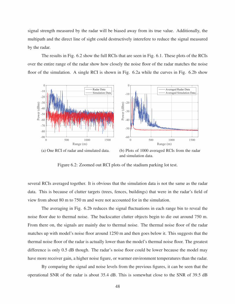
signal strength measured by the radar will be biased away from its true value. Additionally, the

multipath and the direct line of sight could destructively interefere to reduce the signal measured

by the radar.

The results in Fig. 6.2 show the full RCIs that are seen in Fig. 6.1. These plots of the RCIs

over the entire range of the radar show how closely the noise floor of the radar matches the noise

floor of the simulation. A single RCI is shown in Fig. 6.2a while the curves in Fig. 6.2b show

Range (m)0 500 1000 1500

Pow

er (d

Bm

)

-90

-80

-70

-60

-50

-40

-30

-20

-10

0Radar DataSimulation Data

(a) One RCI of radar and simulated data.

Range (m)0 500 1000 1500

Pow

er (d

Bm

)

-60

-50

-40

-30

-20

-10

0Averaged Radar DataAveraged Simulation Data

(b) Plots of 1000 averaged RCIs from the radar

and simulation data.

Figure 6.2: Zoomed out RCI plots of the stadium parking lot test.

several RCIs averaged together. It is obvious that the simulation data is not the same as the radar

data. This is because of clutter targets (trees, fences, buildings) that were in the radar’s field of

view from about 80 m to 750 m and were not accounted for in the simulation.

The averaging in Fig. 6.2b reduces the signal fluctuations in each range bin to reveal the

noise floor due to thermal noise. The backscatter clutter objects begin to die out around 750 m.

From there on, the signals are mainly due to thermal noise. The thermal noise floor of the radar

matches up with model’s noise floor around 1250 m and then goes below it. This suggests that the

thermal noise floor of the radar is actually lower than the model’s thermal noise floor. The greatest

difference is only 0.5 dB though. The radar’s noise floor could be lower because the model may

have more receiver gain, a higher noise figure, or warmer environment temperatures than the radar.

By comparing the signal and noise levels from the previous figures, it can be seen that the

operational SNR of the radar is about 35.4 dB. This is somewhat close to the SNR of 39.5 dB

48

predicted by the radar model. However, the discrepancy of 5 dB between the radar data and the

simulated data noted earlier also factors into the discrepancy in the SNR as well. Thus, there is

some uncertainty in how closely the SNR of the radar compares to its theoretical SNR. Though,

this is still an important observation because it shows that the radar is operating close to design

specifications.

6.2 SAFE-Database Project

The Small Aircraft Flight Encounters (SAFE) Database is a collaborative research project

between Brigham Young University (BYU) and Virginia Polytechnic Institute and State University

(VT) that is funded by the Center for Unmanned Aerial Systems (C-UAS). This research project is

aimed at building a database of flight encounters between small-UAS that includes visual camera

data, aircraft position data, and radar imagery data. BYU’s main contribution to this project was

the radar which was used to gather radar imagery. VT provided small-UAS platforms and cameras.

They also provided a site at Kentland Farm in Blacksburg, VA where flight encounters could be

performed under controlled conditions.

A testing campaign was carried out for this project in August of 2016. The radar was flown

on a fixed-wing aircraft for the first time in these tests. The following subsections describe the tests

done and the results obtained in the campaign.

6.2.1 Equipment Setup

The BYU radar was attached to VT’s eSPAARO fixed-wing UAS during the test encoun-

ters. The radar had three main components which had to be physically attached to the airplane: the

transmit antenna, the receiver antenna array, and the radar’s circuit boards.

The receiver and transmitter were placed on the top and bottom of the fuselage respectively

to reduce coupling between the transmitter and receiver. Figure 6.3 shows what the eSPAARO

looks like and how the antennas were attached to it.

The radar circuit boards were placed inside the fuselage of the eSPAARO. This necessitated

having 3 ft cables go from each of the antennas back into the fuselage to connect to the radar

circuitry. The 3 ft cables used had about 1.5 dB of insertion loss at the operating frequency (10

49

Figure 6.3: The BYU radar attached to VT’s eSPAARO. The receiver and transmitter can be seen

on the top and bottom of the front end of the fuselage.

GHz). This resulted in a loss in transmit power since the power amplifier was also placed inside

the eSPAARO. It also resulted in a loss in the noise figure of the system, bringing it from 3.0 dB

to around 4.5 dB.

The pictures in Fig. 6.4 shows how the radar circuit boards were placed inside the fuselage.

Each of the radar components were first placed on a wood platform as seen in Fig. 6.4a. The

components were attached with tape and foam was also placed underneath the radar stackup to

protect it from vibrations in the eSPAARO.

The platform was mounted inside the eSPAARO’s fuselage as shown in Fig. 6.4b. The

platform helped to keep the radar hardware separate from the eSPAARO’s hardware. The blue RF

cables were fed through a hole in the fuselage to allow the antennas to be connected to the radar.

6.2.2 Flight Campaign Description

Eleven flight encounters were executed during the testing campaign. The missions all in-

volved the eSPAARO using GoPro cameras and the radar to image different targets. The targets of

each mission included a Quanum Nova quad-copter or a Bix3 hobby small-UAS.

50

(a) Platform which held the radar equipment.

Each component starting from the top left and

going to the right is: (1) the power amplifier,

(2) the battery, (3) the radar stackup, and (4) the

power converters.

(b) A picture of the radar inside the eSPAARO.

The blue RF cables connected the radar to the

antennas on the fuselage.

Figure 6.4: Pictures of how the radar was mounted in the eSPAARO.

Each of these encounters had the eSPAARO flying at 100 m above ground level (AGL)

while the target aircraft flew no higher than 70 m in order to maintain a safe spacing distance. This

fact did mean that the targets would be flying towards the edge of the radar’s FOV, which would

result in smaller returns from the target. During each encounter, the radar recorded raw voltage

ADC data. The radar used a slower pulse repetition frequency (PRF) of 200 Hz rather than a PRF

of about 400 Hz because of difficulties with saving all the data from the higher PRF.

Additionally, the GPS data saved by each of the small-UAS in the encounters was used to

synthesize radar data using the simulation model in section 5.3. The following section describes

some important results from the radar which were obtained from the flight campaign.

6.2.3 Flight Campaign Results

The raw ADC data collected by the radar from the encounters showed that (1) the radar

was not sensitive enough to detect the other small-UAS platforms, (2) it is difficult to discriminate

between clutter and UAS that are stationary with respect to the clutter. The simulated radar data

was used to determine where each small-UAS should have been detected.

These results can be illustrated with a few plots. A spectrogram of the radar data obtained

from encounter #1 is shown in Fig. 6.5. A spectrogram shows the power of echoes detected by the

51

Encounter #1

Time17:04:55.577 17:05:03.797 17:05:12.032 17:05:20.196

Ran

ge (m

)

0

200

400

600

800

1000

1200

-70

-65

-60

-55

-50

-45

-40

-35

Figure 6.5: A spectrogram of the radar data from the first encounter.

radar from scatterers within its FOV, neglecting azimuthal information. Time of day appears on

the horizontal axis, range in meters appears on the vertical axis, and the color-map indicates echo

strength in dBm. Thus, a detected scatterer appears as a continuous line of color in the image. This

encounter had the eSPAARO flying at 100 m AGL towards the Quanum Nova which was hovering

at 70 m AGL.

Several targets can be seen in the spectrogram. For instance, the bright band near 100 m

corresponds to the reflection from the ground and represents the altitude of the eSPAARO. The

diagonal streaks in the figure correspond to hard targets such as trees, buildings, and parked cars.

The constant line near 400 m is an artifact of the radar hardware. A signature from the Quanum

Nova cannot be easily identified in Fig. 6.5 because its signature would be changing in range at a

similar rate as other clutter targets. Its signature can be identified though by comparing the radar

data with the simulated radar data.

52

A spectrogram of the simulated radar data generated for encounter #1 is shown in Fig.

6.6. Similar to Fig. 6.5, the vertical axis is range, the horizontal axis is time of day, and color

intensity is mapped to power in dBm. The RCS of the Quanum Nova was assumed to be about

0.05 m2 in order to generate the simulated data. Because the simulation model does not account

for clutter, there is significant difference between Figs. 6.5 and 6.6. The target can be seen in the

data as an approximate hyperbolic curve. The power level of the returns reach about -30 dBm in

the spectrogram.

Encounter #1 Simulation

Time17:04:55.484 17:05:03.484 17:05:11.487 17:05:19.484

Ran

ge (m

)

0

200

400

600

800

1000

1200

-70

-65

-60

-55

-50

-45

-40

-35

Figure 6.6: A spectrogram of simulated radar data from the first encounter.

By comparing the results from the simulation, it is easy to know where to look in Fig. 6.5

to find the Quanum Nova. However, a suitable signature cannot be found. This indicates that

the radar was not able to detect the Quanum Nova. There are two reasons for the absence of the

Quanum Nova’s signature in the radar data. The first and more likely reason is that the radar was

not operating to design specifications, and thus was not sensitive enough to register echoes from

53

the Quanum Nova. The second reason could be that the target may have a smaller RCS than the

estimated value 5 cm2, making it difficult to detect. However, the RCS values given by [19] were

for a small-UAS similar to the Quanum Nova. Therefore, 5 cm2 is a good ball-park number of the

Quanum Nova’s RCS.

The results of the flight campaign were an important step for the radar’s development be-

cause it was the first time the radar had flown on board a small-UAS. They also indicated the

design changes in Chapter 3 needed to be made, which has now allowed the radar to become more

sensitive.

6.2.4 Preliminary Results from Design Changes

The flight results from the SAFE-Database project indicated some needed design changes

in the radar. These changes (see Section 3.2) have made the radar more sensitive. The sensitivity

of the new design was tested in collaboration with the MAGICC lab at BYU. The test was done by

attaching the radar to a X8 Octorotor from the MAGICC as seen Fig. 6.7. It was used to observe

another X8 while both were hovering in the air.

Figure 6.7: A picture of a X8 Octorotor with the radar attached on the bottom.

The X8 that the radar was attached to, known as the ownship, hovered at about 20 m above

ground level (AGL) while another X8, known as the intruder, maneuvered in the radar’s field of

54

view. The radar recorded raw voltage data which was analyzed in post-processing. Figure 6.8

shows a spectrogram of the raw voltage data recorded by the radar. The intruder can be clearly

seen as a diagonal line sloping upward. The horizontal line around 20 m is due to the ground

reflection while the horizontal line at 60 m is an artifact of the radar.

0 0.5 1 1.5 2 2.5

20

40

60

80

100

dBm

-70

-60

-50

-40

-30

-20

Figure 6.8: A Spectrogram plot of the radar data. The radar observed a X8 multicopter from an

airborne platform on board another X8 multicopter.

These preliminary results show that the radar was able to detect another small-UAS up to

80 m away. This is an improvement from the results obtained during the SAFE-Database flight

campaign. However, during this experiment, the intruder was controlled manually and it was

difficult to position the intruder in the radar’s field of view. The experiment was also performed

in a cluttered environment. Future tests could be done where the ownship and intruder follow

programmed waypoints that are designed to keep the intruder in the field of view of the radar.

Future tests could also be done at less cluttered locations.

6.3 Summary

The experiments in this chapter demonstrated the capabilities of the radar. The calibra-

tion tests showed that the radar’s SNR of about 35.4 dB is near the theoretical SNR of 39.5 dB

predicted by the simulation model. The flight tests which were done as part of the SAFE project

55

demonstrated that the radar meets the SWaP requirements of small-UAS. They also uncovered a

potential issue with the radar design because of the radar’s inability to detect small-UAS in its field

of view. This observation prompted a re-design of the radar’s receivers to make it more sensitive.

The preliminary results obtained with the new design have shown that it is more sensitive than the

previous design.

56

CHAPTER 7. CONCLUSION

In recent decades, the microprocessor and computer have ushered in a host of automated

or intelligent tools which complement the lives of people everywhere. These technologies include

things from car navigation systems to word processors. Unmanned aerial systems are a new influ-

ential technology which can enhance life in multiple ways. However, it must be safely integrated

into manned airspace before it can truly become a useful tool. Preparing small-UAS to be aware

of other aircraft and avoid collisions with them is a challenging obstacle.

Using a radar can allow small-UAS to be aware of other aircraft in a non-cooperative en-

vironment, poor-visibility conditions, and in the daytime or nighttime. Radars come with their

own challenges because they often place a high load on the power, space, and payload resources

of small-UAS. However, recent technologies in electronics and processing platforms have allowed

radars to consume less power and become smaller and lighter. The radar described by this doc-

ument and [12] is possible because of these innovations. The contribution of the author to the

creation and testing of the radar included a redesign of its receivers, gathering radar data in the

SAFE Database project, developing an automatic target detection algorithm, and refining a simu-

lation model for the radar.

The creation of a simulation model for the FMCW radar proved to be invaluable. The sim-

ulation model allowed easy development and testing of the signal processing algorithms which run

on the radar’s processing platform. When the radar’s specifications are well measured, the model

also acts as a reference to benchmark the performance of the radar with. Finally, the simulation

model also enabled the creation of synthetic radar data for the SAFE Database project.

The automatic target detection algorithm is an essential part of the radar’s signal processing.

It performs the important task of boiling down the radar’s signals into the location of targets in the

radar’s field of view. By design, the algorithm can adjust to changes in the radar scene using

57

an OS-CFAR algorithm. Testing the algorithm in post-processing has shown that it is capable of

correctly identifying small-UAS as targets of interest in a cluttered environment.

The radar received its first fixed-wing airborne tests during the SAFE Database project.

These tests showed that the radar is capable of meeting the SWaP requirements of small-UAS.

The tests also showed that refinements need to made on the hardware design in order for the radar

to be sensitive enough to detect other small-UAS. The redesign of the radar’s receivers is a step

towards making the radar more sensitive. The redesign allowed the receivers to be more tolerant

of power leaked into the receivers from the transmitter. Testing showed that these design changes

were successful in making the receivers more robust to higher transmit powers.

The progress made on the radar enables it to be a viable part of the solution to the problem

of collision avoidance for small-UAS. The radar meets the strict SWaP requirements of small-UAS.

It has processing algorithms in place which allow it to detect other aircraft. There is a simulation

model that will help benchmark the radar’s performance and assist in the development of any other

processing code. The radar has been flown on a fixed-wing small-UAS and design changes have

been made to its receivers to help make it more sensitive. This progress will be a launch pad for

the future development of this radar and other low SWaP radars for small-UAS.

7.1 Future Work

A few routes for continued progress with the radar are available. These continue the de-

velopment of the radar as a collision avoidance sensor or augment its functionality in substantial

ways.

An important step in the development of the radar as a collision avoidance sensor is to

integrate the radar with the algorithms that decide how to use the data from the radar. The radar

can currently give the range and horizontal bearing to a target. The collision avoidance algorithms

would have to track that target over time and determine if it poses a collision threat. If it does, the

algorithms would have to create a new flight path for the small-UAS to avoid the collision. The

algorithms currently exist (see Section 4.7) and so does the radar. Meshing them together would

be an exciting and challenging avenue for progress.

The current signal processing flow for the radar determines the bearing of targets through a

simple application of DBF. This process forms several beams and the beam with the highest return

58

is designated as the angle of arrival. If a high angular resolution is desired, this method becomes

a cumbersome processing task as many beams must be formed for each range bin. Other methods

such as max SNR beamforming exist that would allow a high angular resolution and may place a

smaller load on the processor than the current method.

Improvements can be made to the radar’s field of view by adding more antenna elements

that will allow the radar to scan in both the horizontal and vertical planes. However, adding more

elements will increase the size of the radar. To keep the radar in the same rough form factor, the

operational frequency of the radar will need to be increased, to 24 GHz for example, so that the

antenna elements can shrink. This would entail a major design project to re-tune all the functional

elements of the radar to work at the new operating frequency.

59

REFERENCES

[1] M. Contarino, “All Weather Sense and Avoid System for UASs,” Report to Office of NavalResearch, R3 Engineering, Scire Consultants, 2009. 2

[2] D. Accardo, G. Fasano, L. Forlenza, A. Moccia, and A. Rispoli, “Flight Test of a Radar-

based Tracking System for UAS Sense and Avoid,” IEEE Transactions on Aerospace andElectronic Systems, vol. 49, no. 2, pp. 1139–1160, 2013. 2

[3] Y. K. Kwag and C. H. Chung, “UAV Based Collision Avoidance Radar Sensor,” in 2007 IEEEInternational Geoscience and Remote Sensing Symposium. IEEE, 2007, pp. 639–642. 2

[4] L. R. Sahawneh, J. Spencer, R. W. Beard, and K. F. Warnick, “Minimum Required Sensing

Range for UAS Sense and Avoid Systems,” AIAA Infotech@ Aerospace, p. 1982, 2016. 2, 40

[5] S. Kemkemian, M. Nouvel-Fiani, P. Cornic, P. Le Bihan, and P. Garrec, “Radar Systems for

Sense and Avoid on UAV,” in 2009 International Radar Conference” Surveillance for a SaferWorld”(RADAR 2009). IEEE, 2009, pp. 1–6. 2

[6] S. Kemkemian, M. Nouvel-Fiani, P. Cornic, and P. Garrec, “MIMO Radar for Sense and

Avoid for UAV,” in Phased Array Systems and Technology (ARRAY), 2010 IEEE Interna-tional Symposium on. IEEE, 2010, pp. 573–580. 2

[7] ——, “A Wide Field of View Radar for Sense and Avoid on UAV Using Space Coloring

Waveforms,” in Radar Conference (EuRAD), 2010 European. IEEE, 2010, pp. 220–223. 2

[8] E. Itcia, J. Wasselin, S. Mazuel, M. Otten, and A. Huizing, “FMCW Radar for the Sense

Function of Sense and Avoid Systems Onboard UAVs,” in SPIE Security+ Defence. Inter-

national Society for Optics and Photonics, 2013, pp. 889 914–889 914. 3

[9] L. Shi, C. Allen, M. Ewing, S. Keshmiri, M. Zakharov, F. Florencio, N. Niakan, and

R. Knight, “Multichannel Sense-and-Avoid Radar for Small UAVs,” in 2013 IEEE/AIAA 32ndDigital Avionics Systems Conference (DASC). IEEE, 2013, pp. 6E2–1. 3

[10] S. M. Duffy, G. A. Brigham, K. S. Newman, P. J. Bell, D. D. Santiago, S. M. Tobin, and

J. S. Herd, “Multi-lithic Phased Array Architecture for Airborne Sense and Avoid Radar,” in

Phased Array Systems & Technology, 2013 IEEE International Symposium on. IEEE, 2013,

pp. 825–830. 3

[11] A. F. Scannapieco, A. Renga, G. Fasano, and A. Moccia, “Ultralight Radar Sensor for Au-

tonomous Operations by Micro-UAS,” in Unmanned Aircraft Systems (ICUAS), 2016 Inter-national Conference on. IEEE, 2016, pp. 727–735. 3

60

[12] J. C. Spencer, “A Compact Phased Array Radar for UAS Sense and Avoid,” Master’s thesis,

Brigham Young University, 2015. vi, vii, 3, 4, 10, 12, 13, 14, 15, 17, 19, 24, 46, 57

[13] M. A. Richards, J. Scheer, W. A. Holm et al., Principles of Modern Radar: Basic Principles.

SciTech Pub., 2010. 6, 32

[14] J. A. Eck, “Compact Antennas and Arrays for Unmanned Air Systems,” Master’s thesis,

Brigham Young University, 2014. 13, 36

[15] L. Newmeyer, D. Wilde, B. Nelson, and M. Wirthlin, “Efficient Processing of Phased Ar-

ray Radar in Sense and Avoid Application Using Heterogeneous Computing,” in Field Pro-grammable Logic and Applications (FPL), 2016 26th International Conference on. EPFL,

2016, pp. 1–8. 22, 23, 26

[16] P. C. Niedfeldt and R. W. Beard, “Convergence and Complexity Analysis of Recursive-

RANSAC: A New Multiple Target Tracking Algorithm,” IEEE Transactions on AutomaticControl, vol. 61, no. 2, pp. 456–461, 2016. 37

[17] L. R. Sahawneh, J. Mackie, J. Spencer, R. W. Beard, and K. F. Warnick, “Airborne Radar-

based Collision Detection and Risk Estimation for Small Unmanned Aircraft Systems,” Jour-nal of Aerospace Information Systems, vol. 12, no. 12, pp. 756–766, 2015. 37

[18] L. R. Sahawneh, M. E. Argyle, and R. W. Beard, “3D Path Planning for Small UAS Oper-

ating in Low-altitude Airspace,” in Unmanned Aircraft Systems (ICUAS), 2016 InternationalConference on. IEEE, 2016, pp. 413–419. 37

[19] C. Tsai, C. Chiang, and W. Liao, “Radar Cross Section Measurement of Unmanned Aerial

Vehicles,” in Electromagnetics: Applications and Student Innovation Competition (iWEM),2016 IEEE International Workshop on. IEEE, 2016, pp. 1–3. 41, 42, 54

[20] F. Ulaby, E. Michielssen, and U. Ravaioli, Fundamentals of Applied Electromagnetics, 6/E.

Pearson Education, Inc., 2010. 44

61