improvements in quantum sdp-solving
TRANSCRIPT

Improvements in Quantum
SDP-Solving
András Gilyén
CWI / QuSoft / University of Amsterdam
June 13, 2018

Optimization is cool

Optimization is cool

Optimization is cool
One of the greatest successes in computer science

Optimization is cool
One of the greatest successes in computer science
Important practical applications in
- Route planning
- Scheduling
- Resource allocation
- Power management
- Design
-...

Quantum optimization?

Quantum optimization?Quantum algorithms for optimization:
Proven advantage
- Grover search
- Quantum Walks
- Backtracking
- Shortest path
- Minimum weight
spanning tree
Heuristics
- Quantum annealing
- Adiabatic algorithms
- QAOA
- VQE
- Quantum machine
learning

Quantum optimization?Quantum algorithms for optimization:
Proven advantage
- Grover search
- Quantum Walks
- Backtracking
- Shortest path
- Minimum weight
spanning tree
Heuristics
- Quantum annealing
- Adiabatic algorithms
- QAOA
- VQE
- Quantum machine
learning
What about Linear Programs (LPs) and Semidefinite
Programs (SDPs)?

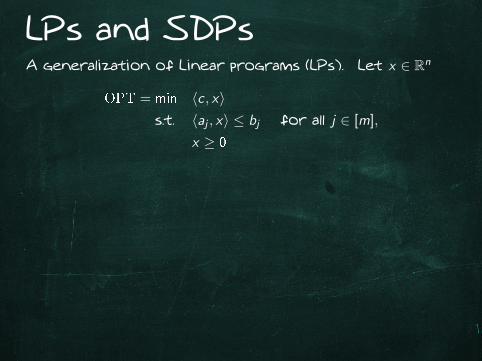
LPs and SDPsA generalization of Linear programs (LPs).

LPs and SDPsA generalization of Linear programs (LPs). Let x ∈ Rn
OPT = min 〈c, x〉
LPs and SDPsA generalization of Linear programs (LPs). Let x ∈ Rn
OPT = min 〈c , x〉s.t. 〈aj , x〉 ≤ bj for all j ∈ [m],
x ≥ 0

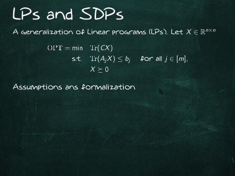
LPs and SDPsA generalization of Linear programs (LPs). Let X ∈ Rn×n
OPT = min 〈C ,X 〉s.t. 〈Aj ,X 〉 ≤ bj for all j ∈ [m],
X ≥ 0
LPs and SDPsA generalization of Linear programs (LPs). Let X ∈ Rn×n
OPT = min Tr(CX )
s.t. Tr(AjX ) ≤ bj for all j ∈ [m],
X 0
Assumptions ans formalization
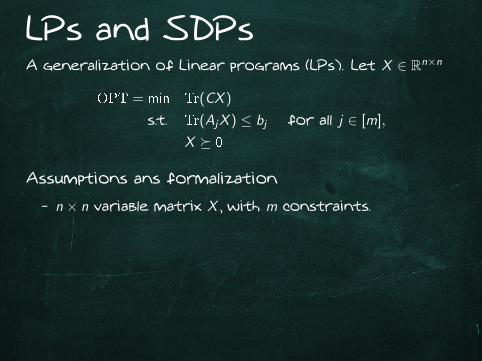
LPs and SDPsA generalization of Linear programs (LPs). Let X ∈ Rn×n
OPT = min Tr(CX )
s.t. Tr(AjX ) ≤ bj for all j ∈ [m],
X 0
Assumptions ans formalization
- n × n variable matrix X , with m constraints.

LPs and SDPsA generalization of Linear programs (LPs). Let X ∈ Rn×n
OPT = min Tr(CX )
s.t. Tr(AjX ) ≤ bj for all j ∈ [m],
X 0
Assumptions ans formalization
- n × n variable matrix X , with m constraints.
- Assume ‖C‖ , ‖Aj‖ ≤ 12
and s-sparse.

LPs and SDPsA generalization of Linear programs (LPs). Let X ∈ Rn×n
OPT = min Tr(CX )
s.t. Tr(AjX ) ≤ bj for all j ∈ [m],
X 0
Assumptions ans formalization
- n × n variable matrix X , with m constraints.
- Assume ‖C‖ , ‖Aj‖ ≤ 12
and s-sparse.
- A priori known bounds Tr (X ) ≤ R and∑m
j=0 yj ≤ r .

LPs and SDPsA generalization of Linear programs (LPs). Let X ∈ Rn×n
OPT = min Tr(CX )
s.t. Tr(AjX ) ≤ bj for all j ∈ [m],
X 0
Assumptions ans formalization
- n × n variable matrix X , with m constraints.
- Assume ‖C‖ , ‖Aj‖ ≤ 12
and s-sparse.
- A priori known bounds Tr (X ) ≤ R and∑m
j=0 yj ≤ r .
- Goal: additive ε-approximation of the optimum.
Examples: MAXCUT, Lovász theta number,
Sum-of-Squares, General Adversary bound, . . .

Classical solvers
- Simplex algorithm for linear programs. (Dantzig, 1947)
- Ellipsoid method in polynomial time. (Khachiyan, 1979)
- Also works for SDPs! (Grötschel, Lovász, Schrijver, 1988)
- State of the art methods: (Lee, Sidford, Wong, 2015)
O(m(m2 + nω + mns) logO(1)(mnR/ε)
),
- Arora and Kale (2008):
Worse error-dependence, better in n and m in certain
cases.

Quantum solversSo far quantum algorithms are based on ideas of Arora-Kale.
Nice speed-ups in n,m but heavy dependence on 1/δ := (Rr)/ε.
- 2016 Sep.: Brandão and Svore: O(√
mns2
δ18
)
- 2017 May.: van Apeldoorn, G., Gribling, de Wolf: O(√
mns2
δ8
)- 2017 Oct.: Brandão, Kalev, Li, Lin, Svore, Wu: O
(√m poly
(B
δ8
))[in a quantum input model]
- 2018 Apr.: Brandão, Kalev, Li, Lin, Svore, Wu: O((√
m +√n) s2δ12
)- 2018 Apr.: van Apeldoorn and G.: O
((√m +
√n) s
δ5
)

Quantum solversSo far quantum algorithms are based on ideas of Arora-Kale.
Nice speed-ups in n,m but heavy dependence on 1/δ := (Rr)/ε.
- 2016 Sep.: Brandão and Svore: O(√
mns2
δ18
)- 2017 May.: van Apeldoorn, G., Gribling, de Wolf: O
(√mn
s2
δ8
)
- 2017 Oct.: Brandão, Kalev, Li, Lin, Svore, Wu: O(√
m poly
(B
δ8
))[in a quantum input model]
- 2018 Apr.: Brandão, Kalev, Li, Lin, Svore, Wu: O((√
m +√n) s2δ12
)- 2018 Apr.: van Apeldoorn and G.: O
((√m +
√n) s
δ5
)

Quantum solversSo far quantum algorithms are based on ideas of Arora-Kale.
Nice speed-ups in n,m but heavy dependence on 1/δ := (Rr)/ε.
- 2016 Sep.: Brandão and Svore: O(√
mns2
δ18
)- 2017 May.: van Apeldoorn, G., Gribling, de Wolf: O
(√mn
s2
δ8
)- 2017 Oct.: Brandão, Kalev, Li, Lin, Svore, Wu: O
(√m poly
(B
δ8
))[in a quantum input model]
- 2018 Apr.: Brandão, Kalev, Li, Lin, Svore, Wu: O((√
m +√n) s2δ12
)- 2018 Apr.: van Apeldoorn and G.: O
((√m +
√n) s
δ5
)

Quantum solversSo far quantum algorithms are based on ideas of Arora-Kale.
Nice speed-ups in n,m but heavy dependence on 1/δ := (Rr)/ε.
- 2016 Sep.: Brandão and Svore: O(√
mns2
δ18
)- 2017 May.: van Apeldoorn, G., Gribling, de Wolf: O
(√mn
s2
δ8
)- 2017 Oct.: Brandão, Kalev, Li, Lin, Svore, Wu: O
(√m poly
(B
δ8
))[in a quantum input model]
- 2018 Apr.: Brandão, Kalev, Li, Lin, Svore, Wu: O((√
m +√n) s2δ12
)
- 2018 Apr.: van Apeldoorn and G.: O((√
m +√n) s
δ5
)

Quantum solversSo far quantum algorithms are based on ideas of Arora-Kale.
Nice speed-ups in n,m but heavy dependence on 1/δ := (Rr)/ε.
- 2016 Sep.: Brandão and Svore: O(√
mns2
δ18
)- 2017 May.: van Apeldoorn, G., Gribling, de Wolf: O
(√mn
s2
δ8
)- 2017 Oct.: Brandão, Kalev, Li, Lin, Svore, Wu: O
(√m poly
(B
δ8
))[in a quantum input model]
- 2018 Apr.: Brandão, Kalev, Li, Lin, Svore, Wu: O((√
m +√n) s2δ12
)- 2018 Apr.: van Apeldoorn and G.: O
((√m +
√n) s
δ5
)

SDP feasibility problem
minTr (CX )
Tr (CX ) ≤ α
Tr (AjX ) ≤ bj for all j ∈ [m]
Tr (X ) = 1
Find X with Tr (X ) = 1 such that
Tr (AjX ) ≤ bj + δ for all j ∈ [m]
or conclude that the problem is infeasible.
[In case the problem is infeasible, but a δ-approximation
exists we allow both solutions.]

SDP feasibility problem
minTr (CX )
Tr (CX ) ≤ α
Tr (AjX ) ≤ bj for all j ∈ [m]
Tr (X ) = 1
Find X with Tr (X ) = 1 such that
Tr (AjX ) ≤ bj + δ for all j ∈ [m]
or conclude that the problem is infeasible.
[In case the problem is infeasible, but a δ-approximation
exists we allow both solutions.]

SDP feasibility problem
minTr (CX )Tr (CX ) ≤ α
Tr (AjX ) ≤ bj for all j ∈ [m]
Tr (X ) = 1
Find X with Tr (X ) = 1 such that
Tr (AjX ) ≤ bj + δ for all j ∈ [m]
or conclude that the problem is infeasible.
[In case the problem is infeasible, but a δ-approximation
exists we allow both solutions.]

SDP feasibility problem
minTr (CX )Tr (CX ) ≤ α
Tr (AjX ) ≤ bj for all j ∈ [m]
Tr (X ) = 1
Find X with Tr (X ) = 1 such that
Tr (AjX ) ≤ bj + δ for all j ∈ [m]
or conclude that the problem is infeasible.
[In case the problem is infeasible, but a δ-approximation
exists we allow both solutions.]

SDP feasibility problem
minTr (CX )Tr (CX ) ≤ α
Tr (AjX ) ≤ bj for all j ∈ [m]
Tr (X ) = 1
Find X with Tr (X ) = 1 such that
Tr (AjX ) ≤ bj + δ for all j ∈ [m]
or conclude that the problem is infeasible.
[In case the problem is infeasible, but a δ-approximation
exists we allow both solutions.]

SDP feasibility problem
minTr (CX )Tr (CX ) ≤ α
Tr (AjX ) ≤ bj for all j ∈ [m]
Tr (X ) = 1
Find X with Tr (X ) = 1 such that
Tr (AjX ) ≤ bj + δ for all j ∈ [m]
or conclude that the problem is infeasible.
[In case the problem is infeasible, but a δ-approximation
exists we allow both solutions.]

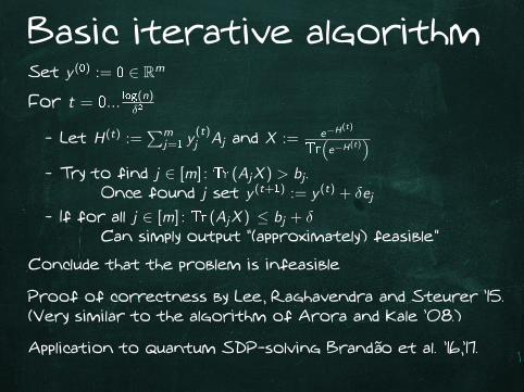
Basic iterative algorithm
Set y (0) := 0 ∈ Rm
For t = 0... log(n)δ2
- Let H(t) :=∑m
j=1 y(t)j Aj and X := e−H(t)
Tr(e−H(t)
)- Try to find j ∈ [m] : Tr (AjX ) > bj .
Once found j set y (t+1) := y (t) + δej
- If for all j ∈ [m] : Tr (AjX ) ≤ bj + δCan simply output “(approximately) feasible”
Conclude that the problem is infeasible
Proof of correctness by Lee, Raghavendra and Steurer ’15.
(Very similar to the algorithm of Arora and Kale ’08.)
Application to quantum SDP-solving Brandão et al. ’16,’17.

Basic iterative algorithmSet y (0) := 0 ∈ Rm
For t = 0... log(n)δ2
- Let H(t) :=∑m
j=1 y(t)j Aj and X := e−H(t)
Tr(e−H(t)
)
- Try to find j ∈ [m] : Tr (AjX ) > bj .Once found j set y (t+1) := y (t) + δej
- If for all j ∈ [m] : Tr (AjX ) ≤ bj + δCan simply output “(approximately) feasible”
Conclude that the problem is infeasible
Proof of correctness by Lee, Raghavendra and Steurer ’15.
(Very similar to the algorithm of Arora and Kale ’08.)
Application to quantum SDP-solving Brandão et al. ’16,’17.

Basic iterative algorithmSet y (0) := 0 ∈ Rm
For t = 0... log(n)δ2
- Let H(t) :=∑m
j=1 y(t)j Aj and X := e−H(t)
Tr(e−H(t)
)- Try to find j ∈ [m] : Tr (AjX ) > bj .
Once found j set y (t+1) := y (t) + δej
- If for all j ∈ [m] : Tr (AjX ) ≤ bj + δCan simply output “(approximately) feasible”
Conclude that the problem is infeasible
Proof of correctness by Lee, Raghavendra and Steurer ’15.
(Very similar to the algorithm of Arora and Kale ’08.)
Application to quantum SDP-solving Brandão et al. ’16,’17.

Basic iterative algorithmSet y (0) := 0 ∈ Rm
For t = 0... log(n)δ2
- Let H(t) :=∑m
j=1 y(t)j Aj and X := e−H(t)
Tr(e−H(t)
)- Try to find j ∈ [m] : Tr (AjX ) > bj .
Once found j set y (t+1) := y (t) + δej
- If for all j ∈ [m] : Tr (AjX ) ≤ bj + δCan simply output “(approximately) feasible”
Conclude that the problem is infeasible
Proof of correctness by Lee, Raghavendra and Steurer ’15.
(Very similar to the algorithm of Arora and Kale ’08.)
Application to quantum SDP-solving Brandão et al. ’16,’17.

Preparing XSuppose we can query the position and value of the non-zero
elements of the sparse matrices Aj , then we can implement
USelect =m∑j=1
|j〉〈j | ⊗ Uj , such that Uj =
[Aj .. .
],
using O (s) queries and gates.

Preparing XSuppose we can query the position and value of the non-zero
elements of the sparse matrices Aj , then we can implement
USelect =m∑j=1
|j〉〈j | ⊗ Uj , such that Uj =
[Aj .. .
],
using O (s) queries and gates.
Let us store y (t) in QRAM using the data structure of
Kerenidis and Prakash. (y (t) is sparse ⇒ QRAM is small.)
USelectLCU=⇒O(1)
[δ∑m
j=1y(t)j Aj .
. .
]

Preparing XSuppose we can query the position and value of the non-zero
elements of the sparse matrices Aj , then we can implement
USelect =m∑j=1
|j〉〈j | ⊗ Uj , such that Uj =
[Aj .. .
],
using O (s) queries and gates.
Let us store y (t) in QRAM using the data structure of
Kerenidis and Prakash. (y (t) is sparse ⇒ QRAM is small.)
USelectLCU=⇒O(1)
[δH(t) .. .
]SVT=⇒O(1/δ)
[e−H
(t)
.. .
]Amp.=⇒O(√n)
X
Preparation of X has O(√
nsδ
)query and time complexity.

Violated constraints
Decide if Tr (AjX ) ≤ bj ± δ
- Can be done using O(
1δ2
)copies of X
- with query and gate complexity O(
sδ2
).
Now we use the quantum OR lemma of Harrow et al. ’17
using its fast implementation due to Brandão et al. ’17.
- Find j ∈ [m] such that Tr (AjX ) ≥ bj- or conclude that for all j ∈ [m] we have Tr (AjX ) ≤ bj + δ
The above problem can be solved with O(
1δ2
)copies of X
with query and gate complexity O(√
msδ2
).
The overall query and gate complexity is O(√
msδ2
+√nsδ3
).

Violated constraints
Decide if Tr (AjX ) ≤ bj ± δ
- Can be done using O(
1δ2
)copies of X
- with query and gate complexity O(
sδ2
).
Now we use the quantum OR lemma of Harrow et al. ’17
using its fast implementation due to Brandão et al. ’17.
- Find j ∈ [m] such that Tr (AjX ) ≥ bj
- or conclude that for all j ∈ [m] we have Tr (AjX ) ≤ bj + δ
The above problem can be solved with O(
1δ2
)copies of X
with query and gate complexity O(√
msδ2
).
The overall query and gate complexity is O(√
msδ2
+√nsδ3
).

Violated constraints
Decide if Tr (AjX ) ≤ bj ± δ
- Can be done using O(
1δ2
)copies of X
- with query and gate complexity O(
sδ2
).
Now we use the quantum OR lemma of Harrow et al. ’17
using its fast implementation due to Brandão et al. ’17.
- Find j ∈ [m] such that Tr (AjX ) ≥ bj- or conclude that for all j ∈ [m] we have Tr (AjX ) ≤ bj + δ
The above problem can be solved with O(
1δ2
)copies of X
with query and gate complexity O(√
msδ2
).
The overall query and gate complexity is O(√
msδ2
+√nsδ3
).

Violated constraints
Decide if Tr (AjX ) ≤ bj ± δ
- Can be done using O(
1δ2
)copies of X
- with query and gate complexity O(
sδ2
).
Now we use the quantum OR lemma of Harrow et al. ’17
using its fast implementation due to Brandão et al. ’17.
- Find j ∈ [m] such that Tr (AjX ) ≥ bj- or conclude that for all j ∈ [m] we have Tr (AjX ) ≤ bj + δ
The above problem can be solved with O(
1δ2
)copies of X
with query and gate complexity O(√
msδ2
).
The overall query and gate complexity is O(√
msδ2
+√nsδ3
).

Applications
Shadow tomography
- Given samples of ρ ∈ Cn×n, and m meas. operators Mj
- find y ∈ Rm such that H :=∑m
j=1 yjMj satisfies
for all j ∈ [m] that
∣∣∣∣Tr (Mjρ)− Tr(Mj
e−H
Tr (e−H)
)∣∣∣∣ ≤ δ.Aaronson showed how to solve using O
(log4(m) log(n)
δ4
)samples.
Our SDP solver recovers it in a gate efficient way
incurring O(√
m)
gate and query complexity overhead.
Further applications
- Quantum state discrimination with maximal total
success probability.
- Optimal measurement design.

Applications
Shadow tomography
- Given samples of ρ ∈ Cn×n, and m meas. operators Mj
- find y ∈ Rm such that H :=∑m
j=1 yjMj satisfies
for all j ∈ [m] that
∣∣∣∣Tr (Mjρ)− Tr(Mj
e−H
Tr (e−H)
)∣∣∣∣ ≤ δ.
Aaronson showed how to solve using O(log4(m) log(n)
δ4
)samples.
Our SDP solver recovers it in a gate efficient way
incurring O(√
m)
gate and query complexity overhead.
Further applications
- Quantum state discrimination with maximal total
success probability.
- Optimal measurement design.

Applications
Shadow tomography
- Given samples of ρ ∈ Cn×n, and m meas. operators Mj
- find y ∈ Rm such that H :=∑m
j=1 yjMj satisfies
for all j ∈ [m] that
∣∣∣∣Tr (Mjρ)− Tr(Mj
e−H
Tr (e−H)
)∣∣∣∣ ≤ δ.Aaronson showed how to solve using O
(log4(m) log(n)
δ4
)samples.
Our SDP solver recovers it in a gate efficient way
incurring O(√
m)
gate and query complexity overhead.
Further applications
- Quantum state discrimination with maximal total
success probability.
- Optimal measurement design.

Applications
Shadow tomography
- Given samples of ρ ∈ Cn×n, and m meas. operators Mj
- find y ∈ Rm such that H :=∑m
j=1 yjMj satisfies
for all j ∈ [m] that
∣∣∣∣Tr (Mjρ)− Tr(Mj
e−H
Tr (e−H)
)∣∣∣∣ ≤ δ.Aaronson showed how to solve using O
(log4(m) log(n)
δ4
)samples.
Our SDP solver recovers it in a gate efficient way
incurring O(√
m)
gate and query complexity overhead.
Further applications
- Quantum state discrimination with maximal total
success probability.
- Optimal measurement design.

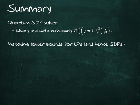
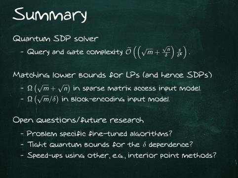
Summary
Quantum SDP solver
- Query and gate complexity O((√
m +√nδ
)sδ4
).
Matching lower bounds for LPs (and hence SDPs)
- Ω(√
m +√n)
in sparse matrix access input model.
- Ω(√
m/δ)
in block-encoding input model.
Open questions/future research
- Problem specific fine-tuned algorithms?
- Tight quantum bounds for the δ dependence?
- Speed-ups using other, e.g., interior point methods?

Sources of images
- c© Lucas Surtin (http://unisci24.com)
- c© Google maps
- c© Gurobi.com
- c© ScienceBuzz.org