improving forecast accuracy by combining recursive and
TRANSCRIPT

Preliminary and incomplete Improving Forecast Accuracy by Combining Recursive and Rolling Forecasts
Todd E. Clark and Michael W. McCracken* Federal Reserve Bank of Kansas City and University of Missouri-Columbia
July 2004
Abstract This paper presents analytical, Monte Carlo, and empirical evidence on the effectiveness of combining recursive and rolling forecasts, compared to using either just a recursive or rolling forecast, when linear predictive models are subject to structural change. We first provide a characterization of the bias-variance tradeoff faced when choosing between either the recursive and rolling schemes or a scalar convex combination of the two. From that, we derive pointwise optimal time-varying and data dependent observation windows and combining weights designed to minimize mean square forecast error. We then proceed to consider other methods of forecast combination including Bayesian methods that shrink the rolling forecast to the recursive and Bayesian model averaging. Monte Carlo experiments and several empirical examples indicate that although the recursive scheme is often difficult to beat, when gains can be obtained, some form of shrinkage can often provide improvements in forecast accuracy relative to forecasts made using the recursive scheme or the rolling scheme with a fixed window width. Keywords: structural breaks, forecasting, model averaging. JEL Nos.: C53, C12, C52 *Clark: Economic Research Dept., Federal Reserve Bank of Kansas City, 925 Grand Blvd., Kansas City, MO 64198, [email protected]. McCracken (corresponding author): Dept. of Economics, University of Missouri-Columbia, 118 Professional Building, Columbia, MO 65211, [email protected]. We gratefully acknowledge the excellent research assistance of Taisuke Nakata and helpful comments from Ulrich Muller, Jonathan Wright and participants at the following meetings: MEG, Canadian Economic Assocation, SNDE, MEA, and the conference for young researchers on Forecasting in Time Series. The views expressed herein are solely those of the authors and do not necessarily reflect the views of the Federal Reserve Bank of Kansas City or the Federal Reserve System

1
1. Introduction
In a universe characterized by heterogeneity and structural change, forecasting agents may
feel it necessary to estimate model parameters using only a partial window of the available
observations. The intuition is clear. If the earliest available data follow a data-generating
process unrelated to the present then using such data to estimate model parameters may lead to
biased parameter estimates and forecasts. Such biases can accumulate and lead to larger mean
square forecast errors than do forecasts constructed using only that data relevant to the present
and (hopefully) future data-generating process. Unfortunately, if we reduce the number of
observations in order to reduce heterogeneity we simultaneously increase the variance of the
parameter estimates. This increase in variance maps into the forecast errors and causes the mean
square forecast error to increase. Hence when constructing a forecast there is a balance between
using too much or too little data to estimate model parameters.
This tradeoff leads to patterns in the decisions on whether or not to use all available data
when constructing forecasts. As noted in Giacomini and White (2003), the finance literature
tends to construct forecasts using only a rolling window of the most recent observations. In the
macroeconomics literature, it is more common for forecasts to be constructed recursively – using
all available data to estimate unknown parameters (e.g. Stock and Watson, 2003a) – with
forecasts only sometimes based on rolling windows. Since both macroeconomic and financial
series are known to exhibit periods of structural change (Stock and Watson 1996, Paye and
Timmermann 2002), one reason for the rolling approach to be used more often in finance than in
macroeconomics may simply be that financial series are often substantially longer. This allows
individuals who forecast financial series to make choices to reduce the bias component of the

2
bias-variance tradeoff that macroeconomic forecasters often cannot make due to the potentially
sharp deterioration in the variance component of the tradeoff.
In light of the bias-variance tradeoff associated with the choice between a rolling and
recursive forecasting scheme, a combination of recursive and rolling forecasts could be superior
to the individual forecasts. Indeed, combining recursive and rolling forecasts could be
interpreted as yet another form of shrinkage estimation that might be useful in the presence of
instabilities. The findings of Min and Zellner (1993), Koop and Potter (2003), Stock and Watson
(2003), and Wright (2003) suggest shrinkage (the particular forms vary across these studies) to
be effective in samples with instabilities.
Accordingly, we present analytical, Monte Carlo, and empirical evidence on the effectiveness
of combining recursive and rolling forecasts, compared to using either just a recursive or rolling
forecast. We first provide a characterization of the bias-variance tradeoff involved in choosing
between either the recursive and rolling schemes or a scalar convex combination of the two.
This tradeoff permits us to derive not only optimal observation windows for the rolling scheme
but, given a rolling observation window, the optimal scalar weights for combining the recursive
and rolling schemes.
Because we find that simple scalar methods of combining the recursive and rolling forecasts
are useful, we also consider combining methods that do not fit directly into our analytical
framework. One approach uses standard Bayesian methods to shrink parameter estimates based
on a rolling sample toward those based on the recursive sample. Another method consists of
using the Bayesian model averaging approach of Wright (2003) to average a recursive forecast
with a sequence of rolling forecasts, each with a distinct observation window.

3
The results in the paper suggest a benefit to some form of combination of recursive and
rolling forecasts. Our Monte Carlo and empirical results show that shrinking coefficient
estimates based on a rolling window of data seems to be effective and valuable. On average, the
shrinkage produces a forecast MSE essentially the same as the recursive MSE when the recursive
MSE is best. When there are model instabilities, the shrinkage produces a forecast MSE that
often captures most of the gain that can be achieved with the methods we consider. Thus
combining recursive and rolling forecasts yields forecasts that are likely to be as good as or
better than either recursive or rolling forecasts based on an arbitrary, fixed window size.
Our results build on several lines of extant work. First, we build on the very large literature
on forecast combination, a subject that has recently seen renewed interest, both theoretical (e.g.
Elliott and Timmermann, 2003) and empirical (e.g. Stock and Watson, 2003a,b). Second, our
analysis follows very much in the spirit of Min and Zellner (1993), who also consider forecast
combination as a means of handling heterogeneity induced by structural change. Using a
Bayesian framework, they combine a stable linear regression model with another with classical
unit-root time variation in the parameters.
Finally, our work on the optimal choice of observation window builds on Pesaran and
Timmermann (2002). They, too, consider the determinants of the optimal choice of the
observation window in a linear regression framework subject to structural change. Using both
conditional and unconditional mean square errors as objective functions they find that the
optimal length of the observation window is weakly decreasing in the magnitude of the break,
weakly decreasing in the magnitude of any change in the residual variance and is weakly
increasing in the magnitude of the time since the break date. They derive a recursive data-based
stopping rule for selecting the observation window that does not admit a closed-form solution.

4
We are able to generalize Pesaran and Timmermann’s results in many respects – among them,
imposing less restrictive assumptions, such as a scalar parameter vector, and obtaining closed
form solutions for the optimal window size.
Our paper proceeds as follows. In section 2 we analytically characterize the bias-variance
tradeoff and, in light of that tradeoff, determine the optimal observation window. Section 3
details the recursive-rolling combination methods considered. In section 4 we present Monte
Carlo evidence on the finite sample effectiveness of our combination approaches and various
other methods for forecasting in the potential presence of model instability. Section 5 compares
the effectiveness of the various forecast methods approaches in a range of empirical applications.
The final section concludes. Various details pertaining to theory and data are presented in
Appendixes 1 and 2.
2. Analytical Results on the Bias-Variance Tradeoff and Optimal Observation Window
In this section, after first detailing the necessary notation, we provide an analytical
characterization of the bias-variance tradeoff, created by model instability, involved in choosing
between recursive and rolling forecasts. In light of that tradeoff, we then derive the optimal
rolling observation window. A detailed set of technical assumptions, sufficient for the results,
are given in Appendix 1. The same appendix provides general theoretical results (allowing for
the recursive and rolling forecasts to be combined with weights αt and 1- αt respectively) from
which the results in this section are derived as a special case (with αt = 0). We take up the
possibility of combining the recursive and rolling forecasts in section 3.
2.1 Environment
The possibility of structural change is modeled using a sequence of linear DGPs of the form

5
yT,t+τ = ' *
T,t T,tx β + ut+τ,T *T,tβ = β* + T-1/2g(t/T)
ExT,tuT,t+τ ≡ EhT,t+τ = 0 for all t = 1,…,T,…,T+P.
Note that the dependent variable yT,t+τ, the predictors xT,t and the error term uT,t+τ all depend upon
T, the initial forecasting origin. This is certainly necessary for the dependent variable since it
depends upon the sequence of parameter vectors *T,tβ which in turn depend upon T. We allow
the predictors and the errors to depend upon T because we do not want to make the strong
assumption that these terms are strongly exogenous to the process generating the dependent
variable. By doing so we allow the time variation in the parameters to have some influence on
their marginal distributions. This is necessary if we want to allow lagged dependent variables to
be predictors.
Except where necessary, however, for the remainder we omit the subscript T that is
associated with the observables and the errors. Ultimately, the dependence of the observable
variables and their marginal distributions on T is not particularly important when the sample size
is large. With linear models subject to local structural change and test statistics formed using
sample averages of quadratics of the predictors and forecast errors, we are able to take advantage
of the concept of asymptotic mean square stationarity as discussed in Hansen (2000). In
Appendix 1 we reintroduce the dependence of the observables upon T and more formally keep
track of its impact on the bias-variance tradeoff.
At each origin of forecasting t = T,…, T+P, we observe the sequence ' tj j j 1y , x = . These
include a scalar random variable yt to be predicted and a (k×1) vector of potential predictors xt
which may include lagged dependent variables. Forecasts of the scalar yt+τ, t = T,…,T+P τ ≥ 1,
6
are generated using the vector of covariates xt and the linear parametric model 'tx β . The
parameters are estimated one of two ways. For a time varying observation window Rt, the
parameter estimates satisfy R,tβ = argmin -1 ' 2t-s=1 s+ st (y -x β)τ
τ∑ and L,tβ = argmin
t
-1 ' 2t-s=t- -R +1t s+ sR (y -x β)τ
τ τ∑ for the recursive and rolling schemes respectively. The corresponding
loss associated with the forecast errors are 2R,tu +τ = ' 2
t+ t R,tˆ(y -x β )τ and 2
L,tu +τ = ' 2t+ t L,t
ˆ(y -x β )τ .
Before presenting the results it is useful to provide a brief discussion of Assumptions 1–4 in
Appendix 1. In Assumptions 1–3 we maintain that the OLS-estimated DGP is a linear regression
subject to local structural change. The local structural change is nonstochastic, square integrable
and of a small enough magnitude that the observables are asymptotically mean square stationary.
In order to insure that certain weighted partial sums converge weakly to standard Brownian
motion W(.), we impose the high level assumption that, in particular, ht+τ satisfies Theorem 3.2
of De Jong and Davidson (2000). By doing so we also are able to take advantage of various
results pertaining to convergence in distribution to stochastic integrals that are also contained in
De Jong and Davidson.
Our final assumption is unique. In part (a) of Assumption 4 we generalize assumptions made
in West (1996) that require limT→∞Rt/T = λR ∈ (0, 1). Such an assumption is too stringent for
our goals. Instead, in parts (a) and (c) we weaken that type of assumption so that Rt/T ⇒ λR(s)∈
(0, s], 1 ≤ s ≤ 1 + λP, where limT→∞P/T = λP ∈ (0, ∞) and hence the duration of forecasting is
finite but non-trivial. By doing so we permit an observation window that changes with time as
evidence of instability is discovered. For the moment we omit a discussion of part (b) but return
to it in section 3 when we consider combining the recursive and rolling schemes.

7
2.2 Theoretical results on the tradeoff: the general case
Our approach to understanding the bias-variance tradeoff is based upon an analysis of
2 2T Pt T R,t+ L,t+ˆ ˆ(u -u )+= τ τ∑ , the difference in the (normalized) MSEs of the recursive and rolling
forecasts.1 As detailed in Theorem 1 in Appendix 1, we show that this statistic has an asymptotic
distribution that can be decomposed into three terms:
2 2T P
t T R,t+ L,t+ˆ ˆ(u -u )+= τ τ∑ →d P1
W1 (s)+λ ξ∫ = P1W11 (s)+λ ξ∫ + P1
W21 (s)+λ ξ∫ + P1W31 (s)+λ ξ∫ . (1)
The first component can be interpreted as the pure “variance” contribution to the distribution of
the difference in the recursive and rolling MSEs. The third term can be interpreted as the pure
“bias” contribution, while the second is an interaction term.
This very general result implies that the bias-variance tradeoff depends on: (1) the rolling
window size (λR(s)), (2) the duration of forecasting (λP), (3) the dimension of the parameter
vector (through the dimension of W or g), (4) the magnitude of the parameter variability (as
measured by the integral of quadratics of g), (5) the forecast horizon (as measured by the long-
run variance of ht+τ, V) and (6) the second moments of the predictors (B = limT→∞' -1
T,t T,t(Ex x ) ).
Providing a more detailed analysis of the distribution of the relative accuracy measure is
difficult because we do not have a closed form solution for the density and the bias term allows
for very general breaking processes. Therefore, we proceed in the remainder of this section to
focus on the mean (rather than the distribution) of the bias-variance tradeoff when there are
either no breaks or a single break.
1 In Theorem 1, the tradeoff is based on 2 2T P
t T R,t+ W,t+ˆ ˆ(u -u )+= τ τ∑ , which depends upon the combining weights αt. If we
set αt = 0 we find that 2 2T Pt T R,t+ W,t+ˆ ˆ(u -u )+= τ τ∑ = 2 2T P
t T R,t+ L,t+ˆ ˆ(u -u )+= τ τ∑ .

8
2.3 The case of no break
We can precisely characterize the mean in the case of no breaks. When there are no breaks
we need only analyze the mean of the variance contribution P1W11 (s)+λ ξ∫ . Taking expectations
and noting that the first of the variance components is zero mean we obtain
P1W11 E (s)+λ ξ∫ = P1+λ
1R
1 1tr(BV) ( - )dss λ (s)∫ (2)
where tr(.) denotes the trace operator. It is straightforward to establish that all else constant, the
mean variance contribution is increasing in the window width λR(s), decreasing in the forecast
duration λP and negative semi-definite for all λP and λR(s). Not surprisingly, we obtain the
intuitive result that in the absence of any structural breaks the optimal observation window is
λR(s) = s. In other words, in the absence of a break it is always best to use the recursive scheme.
2.4 The case of a single break
Suppose that a permanent local structural change, of magnitude T-1/2g(t/T) = T-1/2∆β, in the
parameter vector β occurs at time 1 ≤ TB ≤ t where again, t = T,…, T+P denotes the present
forecasting origin. In the following let limT→∞TB/T = λB ∈ (0, s). Substitution into Theorem 1 in
Appendix 1 yields the following corollary regarding the bias-variance tradeoff.
Corollary 2.1: (a) If λR(s) > s − λB for all s ∈ [1,1+λP] then
P1W1 E (s)+λ ξ∫ = P1+λ
1R
1 1tr(BV) ( - )dss λ (s)∫
+ P1+λ' -1 B R RR B1 2 2
R
-(s-λ )(s+ (s))+2sλ (s)∆βB ∆β (s- (s))(s-λ )( )dss λ (s)λ
λ∫ .

9
(b) If λR(s) ≤ s − λB for all s ∈ [1,1+λP] then
P1W1 E (s)+λ ξ∫ = P1+λ
1R
1 1tr(BV) ( - )dss λ (s)∫ + P
21+λ' -1 B1 2
λ∆βB ∆β ( )dss∫ .
From Corollary 2.1 we see that the tradeoff depends upon a weighted average of the
precision of the parameter estimates as measured by tr(BV) and the magnitude of the structural
break as measured by the quadratic ' -1∆βB ∆β . Note that the first term in each of the expansions
is negative semi-definite while that for the latter is positive semi-definite. Intuitively, we would
expect this to imply that as the magnitude of the break increases relative to the precision of the
parameter estimates it is optimal to decrease the observation window.
Even so, part (b) of Corollary 2.1 places a bound on the amount that one would be willing to
decrease the width of the observation window. This can be seen if we notice that the bias
component does not depend upon the magnitude of the observation window − except for the
condition that it be less than or equal to s − λB. Since the variance component is monotone
increasing in λR(s) we immediately conclude that it is never optimal to choose an observation
window less than the entirety of the sample since the most recent break.
Although it is perhaps not immediately obvious, Corollary 2.1 does not consider all possible
choices of λR(s). There are three possibilities. In the first the window always is large enough to
include the break date. In the second the window is never big enough to contain observations
prior to the break date. In the third, the window is allowed to sometimes capture the break date
but sometimes not. We do not consider the third case since it is irrelevant towards our goal of
optimizing over the bias-variance tradeoff. This follows from our intuitive discussion of part (b)
of Corollary 2.1 and is stated explicitly in the following corollary.

10
Corollary 2.2: In the presence of a single break in the regression parameter vector, the pointwise
optimal observation window satisfies
*R (s)λ =
' -1
B B2 ' -1
B
B BB ' -1
B B
s ∆βB ∆βs2λ (s-λ ) tr(BV)
2(s-λ ) s ∆βB ∆β<tr(BV) 2λ (s-λ ) tr(BV)2(s-λ )-( )∆βB ∆β
s-λ s-λ
⎧≥⎪
⎪⎪⎪⎨⎪⎪⎪ → ∞⎪⎩
.
Corollary 2.2 provides pointwise optimal observation windows for forecasting in the
presence of a single structural change in the regression coefficients. We describe these as
pointwise optimal because they are derived by maximizing the individual elements from part (a)
of Corollary 2.1 that contribute to the average expected mean square differential over the
duration of forecasting. In other words, the results of Corollary 2.2 follow from maximizing
R
1 1tr(BV)( - )s λ (s)
+ ' -1 B R RR B 2 2
R
-(s-λ )(s+ (s))+2sλ (s))∆βB ∆β(s- (s))(s-λ )( )s λ (s)λ
λ (3)
with respect to λR(s) for each s. Again, we do not need to consider the case in which λR(s) is
ever less than s − λB since, as can be seen from part (b) of Corollary 2.1, any time period in
which λR(s) < s − λB monotonically reduces the objective function.
The formula in Corollary 2.2 is plain enough that comparative statics are reasonably simple.
Perhaps the most important is that the observation window is increasing in the ratio
' -1tr(BV)/∆βB ∆β . For smaller breaks we expect to use a larger observation window and when
parameter estimates are more precisely estimated (so that tr(BV) is small) we expect to use a
smaller observation window.

11
Note, however, that the term ' -1∆βB ∆β is a function of the local break magnitudes ∆β and
not the global break magnitudes we estimate in practice. Moreover, note that these optimal
windows are not presented relative to an environment in which agents are forecasting in ‘real
time’. Taken literally, if we were to use the formulas we would need to know the original
forecasting origin T and estimate quantities like s and λB using s = t/T and Bλ = BT /T for an
estimated break date BT .
Rather than take this approach we suggest a transformed formula that treats the present
forecasting origin as the only one that is relevant. Let B and V denote estimates of B and V
respectively. If for an estimated global break ˆ∆β at an estimated break date BT , we let
ˆ∆β denote an estimate of the local change in β (∆β/T1/2) at time TB and t/TˆBB =δ , we obtain the
following real time estimate of the pointwise optimal observation window.2
*tR =
' -1
B B
2 ' -1B
B BB ' -1
B B
ˆ ˆˆ1 t∆βB ∆βt ˆ ˆ ˆ ˆtr(BV)2 (1- )ˆ ˆˆ ˆ2t(1- ) 1 t∆βB ∆β<ˆ ˆ ˆ ˆ ˆ ˆtr(BV) tr(BV)2 (1- )ˆ2(1- )-( )ˆ ˆˆt∆βB ∆β
ˆ ˆt(1- ) 1 1
⎧≥⎪
δ δ⎪⎪ δ⎪⎨
δ δ⎪ δ⎪⎪⎪ δ − δ →⎩
. (4)
2 We estimate B with -1 ' -1t
j 1 j jB=(t x x )=∑ , where xt is the vector of regressors in the forecasting model (supposing the MSE stationarity assumed in the theoretical analysis. In the Monte Carlo experiments, tr(BV)is estimated imposing homoskedasticity: tr(BV) = 2ˆkσ , where k is the number of regressors in the forecasting model and 2σ is the estimated residual variance of the forecasting model estimated with data from 1 to t. In the empirical applications, though, we use the estimate tr(BV) = -1 ' -1 -1 2 't t
j=1 j=1j j j+ j jˆtr[(t x x ) (t u x x )]τ∑ ∑ , where u refers to the residuals from estimates of the forecasting model using data from 1 to t.

12
One final note on the formulae in Corollary 2.2 and (4). In Corollary 2.2, we use local breaks
to model the bias-variance tradeoff faced by a forecasting agent in finite samples. By doing so
we are able to derive closed form solutions for the optimal observation window. Unfortunately,
by taking this approach we have created a situation where we have no choice but to use
inconsistent (Bai (1997)) global break magnitudes and dates to estimate the assumed local
magnitudes. Not surprisingly, in our Monte Carlo results we find that experiments which treat
the break magnitudes and dates as known perform better than other experiments where we
estimate these quantities. Even so, we find that the estimated quantities perform well enough to
be a valuable tool for forecasting.
3. Approaches to Combining Recursive and Rolling Forecasts
In section 2 we discussed how the choice of observation window can improve forecast
accuracy by appropriately balancing a bias-variance tradeoff. In this section, we consider
whether combining recursive and rolling forecasts can also improve forecast accuracy by
balancing a similar tradeoff. We do so using three different combination approaches. The first is
a simple scalar combination of recursive and rolling forecasts. The second, which can be viewed
as a matrix-valued combination, is based on Bayesian shrinkage of rolling model estimates
toward recursive estimates. The third relies on Bayesian model averaging, as implemented in
Wright (2003).
3.1 Simple scalar combination
The simplest possible approach to combination is to form a scalar linear combination of
recursive and rolling forecasts. With linear models, of course, the linear combination of the
forecasts is the same as that generated with a linear combination of the recursive and rolling

13
parameter estimates. Accordingly, we consider generating a forecast using coefficients W,tβ =
αt R,tβ + (1−αt) L,tβ , with corresponding loss 2W,tu +τ = ' 2
t+ t W,tˆ(y -x β )τ . The size of the observation
window used by the rolling coefficient estimates L,tβ could be set arbitrarily at, say, 40
observations, or it could be chosen to produce the lowest possible MSE of the combined forecast.
Using Theorem 1 in Appendix 1, we are able to derive these optimal combining weights in
the presence of a single structural break. Moreover, we are able to generalize the analytical
results from Corollary 2.2 on the optimal observation window to an environment in which we
choose the optimal observation window for a given combining weight. If, as we have for the
observation window Rt, we let αt converge weakly to the function α(s), the following corollaries
provide the desired results. For each we maintain the same assumptions and notation used in
Corollaries 2.1 and 2.2.
Corollary 3.1: (a) If λR(s) > s − λB for all s ∈ (1, 1+λP] then
P1W1 E (s)+λ ξ∫ = P1+λ 2
1R
1 1tr(BV) (1- (s)) ( - )dss λ (s)
α∫
+ P1+λ' -1 B R R RR B1 2 2
R
(s-λ )( (s)(s- (s))-(s+ (s)))+2sλ (s))∆βB ∆β (1-α(s))(s- (s))(s-λ )( )dss λ (s)
α λ λλ∫ .
(b) If λR(s) ≤ s − λB for all s ∈ (1, 1+λP] then
P1W1 E (s)+λ ξ∫ = P1+λ 2
1R
1 1tr(BV) (1-α(s)) ( - )dss λ (s)∫ + P
21+λ' -1 2 B1 2
λ∆βB ∆β (1-α (s))( )dss∫ .
Corollary 3.2: In the presence of a single break in the regression parameter vector, the pointwise
optimal window width and combining weights satisfy

14
*R (s, (s))λ α =
' -1
B B2 ' -1
B
B BB B ' -1
B B
s(1- (s)) ∆βB ∆βs2λ (s-λ ) tr(BV)
2s(1-α(s))(s-λ ) s(1- (s)) ∆βB ∆β<tr(BV) 2λ (s-λ ) tr(BV)2(s-λ )(s-α(s)(s-λ ))-s(1-α(s))( )∆βB ∆β
s-λ s-λ
⎧ α≥⎪
⎪⎪ α⎪⎨⎪⎪⎪ → ∞⎪⎩
and for λR(s) > s–λB
*R(s, (s))α λ =
' -1
R B B R 2B
R' -12
B ' -1R B R
2B
R
B ' -1
∆βB ∆βs (s)+( )s(s-λ )(s-λ -λ (s))(s- )tr(BV) (s)tr(BV)∆βB ∆β (s- )-( )s (s)+( )(s-λ ) (s-λ (s)) ∆βB ∆βtr(BV)(s- )0 (s)tr(BV)(s- )-( )∆βB ∆β
⎧λ⎪ λ⎪ ≥ λ
⎪ λλ⎪⎨⎪ λ⎪ < λ⎪ λ⎪⎩
.
The Corollary provides pointwise optimal observation windows and combining weights for
forecasting in the presence of a single structural change in the regression coefficients. As was
the case in Corollary 2.2, we describe these as pointwise optimal because they are derived by
maximizing the individual elements from part (a) of Corollary 3.1. Again, we do not need to
consider the case in which λR(s) is ever less than s − λB since any time period in which λR(s) < s
− λB monotonically reduces the objective function.
The formula for the optimal observation window λR(s), for a given combining weight α(s), is
very closely related to that from Corollary 2.2. Perhaps the largest difference between the two is
that the observation window on the rolling component is more likely to be smaller since the bias-
variance tradeoff is affected by the fact that some weight (α(s) > 0) is being placed on the
recursive forecast. Comparative statics for the combining weights are also relatively
straightforward. As the observation window on the rolling component increases, we place less

15
weight on the recursive scheme. Similarly, as the magnitude of the break increases relative to
the precision of the parameter estimates, we also place less weight on the recursive scheme.
Finally, we obtain the intuitive result that as the time since the break increases (s–λB), we
eventually place all weight on the rolling scheme.
As was the case for the formula from Corollary 2.2, the optimal observation windows and
combining weights in Corollary 3.2 are not presented in a real time context and depend upon
several unknown quantities. If we make the same change of scale and use the same estimators
that were used for equation (4), we obtain the real time equivalents of the formulas from
Corollary 3.2.
*t tR (α ) =
' -1t
B B
2 ' -1t B t
B BB t B t ' -1
B B
ˆ ˆˆ(1- ) t∆βB ∆βt ˆ ˆ ˆ ˆtr(BV)2 (1- )ˆ ˆˆ ˆ2t(1-α )(1- ) (1- ) t∆βB ∆β<ˆ ˆ ˆ ˆ ˆ ˆtr(BV) tr(BV)2 (1- )ˆ ˆ2(1- )(1-α (1- ))-(1-α )( )ˆ ˆˆt∆βB ∆β
ˆ ˆt(1- ) 1 1
⎧ α≥⎪
δ δ⎪⎪ δ α⎪⎨
δ δ⎪ δ δ⎪⎪⎪ δ − δ →⎩
(5)
and
*t tˆ (R )α =
' -1
t B B t 2B
t' -12
Bt B t ' -1
2B
t
B ' -1
ˆ ˆˆt∆βB ∆β ˆ ˆ(R /t)+( )(1-δ )(1-δ -(R /t)) ˆˆ ˆ t(1-δ )tr(BV) Rˆ ˆ ˆ ˆˆ tr(BV)t∆βB ∆β ˆˆ (1-δ )-( )(R /t)+( )(1-δ ) (1-(R /t)) ˆ ˆˆ ˆ ˆtr(BV) t∆βB ∆βˆt(1-δ )0 Rˆ ˆtr(BV)ˆ(1-δ )-( )ˆ ˆˆt∆βB ∆β
⎧⎪⎪ ≥⎪⎪⎨⎪⎪ <⎪⎪⎩
. (6)
One final note on Corollary 3.2. The optimal solutions for the observation window λR(s) and
combining weight α(s) are each derived conditioning on the other. An alternative approach

16
would be to derive the jointly optimal observation and combining weights. We have attempted
to do so but jointly determining both optimal values does not appear readily tractable.
3.2 A Bayesian shrinkage forecast
Given the bias-variance tradeoff between recursive and rolling forecasts, a second
combination approach that might seem natural is to use parameter estimates based on a rolling
sample shrunken so as to reduce the noise in the parameter estimates and resulting forecast. We
therefore consider shrinking rolling sample estimates toward the recursive estimates,
implemented with standard Bayesian formulae. Recall that for a prior β ~ N(m, σ2M), the
Normal linear regression model yields the posterior maximizing estimate β =
-1 -1 -1(M +X X) (M m+X Y)′ ′ where X denotes the relevant design matrix and Y the associated
vector of dependent variables. If we treat the recursive parameter estimates as the prior mean
and treat the associated standard errors under conditional homoskedasticity as our prior variance
we have m = R,tβ and M = -1RB (t) where RB (t) = -1 ' -1t-τ
j=1 j j(t x x )∑ . If we let LB (t) =
t
-1 ' -1t-τj=t-τ-R +1t j j(R x x )∑ , our Bayesian shrinkage estimator then follows by constructing the posterior
maximizing rolling parameter estimates given this prior:
W,tβ = [tBR(t)-1 + RtBL(t)-1]-1[tBR(t)-1
R,tβ +t
t-s=t- -R +1 s s+x yτ
τ τ∑ ]
= [BR(t)-1 + (Rt/t)BL(t)-1]-1BR(t)-1R,tβ + [(t/Rt)BR(t)-1 + BL(t)-1]-1BL(t)-1
L,tβ . (7)
It is clear from the right-hand side of (7) that the parameter estimates are a linear combination of
both recursive and rolling parameter estimates. In contrast to the simple combination considered
in our analytical work, here the weights are matrix valued and depend upon the ratio Rt/t and the
matrices of sample second moments BR(t) and BL(t).

17
This Bayesian shrinkage estimator of course involves selecting a rolling observation window.
One approach is to use an arbitrary window of, say, 40 observations. Another approach is to
exploit the fact that the shrinkage estimator (7) can be fit into our general analytical framework,
and use the appropriate optimal window. Under the assumption of asymptotic mean square
stationarity, our Bayesian shrinkage estimator is asymptotically equivalent to a scalar-weighted
combination of recursive and rolling estimators, with combination weights αt = t/(t + Rt) and (1 −
αt) = Rt/(t + Rt):
W,tβ = [BR(t)-1 + (Rt/t)BL(t)-1]-1BR(t)-1
R,tβ + [(t/Rt)BR(t)-1 + BL(t)-1]-1BL(t)-1L,tβ (8)
~ [1 + (Rt/t)]-1R,tβ + [(t/Rt) + 1]-1
L,tβ
= R,tt
t ˆ( )βt+R
+ tL,t
t
R ˆ( )βt+R
.
To obtain the asymptotically optimal observation window associated with these weights we
need only substitute these weights into our formula from equation (5) . Doing so we find that
*t tR (t/(t+R )) =
' -1
B B
2 ' -1B B
B B BB ' -1
' -1
BB
ˆ ˆˆ1 t∆βB ∆βt ˆ ˆ ˆ ˆtr(BV)4 (1- )ˆ ˆˆ ˆ ˆ ˆ2t[(1- ) (1- )] 1 t∆βB ∆β 1<ˆ ˆ ˆ ˆ ˆ ˆ ˆtr(BV) tr(BV)4 (1- ) 2ˆ2(1- )-( )ˆ ˆˆt∆βB ∆β
ˆ ˆˆt∆βB ∆β 1ˆt(1- ) ˆ ˆ ˆtr(BV) 2
⎧⎪⎪ ≥⎪ δ δ⎪⎪ δ − δ δ
<⎨δ δ δ⎪ δ
⎪⎪⎪
δ ≥⎪ δ⎩
. (9)
The formula in (9) is very close to that in (4) when αt = 0, but with one important difference.
We are less likely to have a solution where Rt is close to t and much more likely to have a

18
solution where Rt = Bˆt(1- )δ . Since the Bayesian shrinkage method always places some weight
on the recursive component it is not surprising that the observation window for the rolling
component of the shrinkage estimator is smaller than that for the pure rolling (αt = 0) scheme.
3.3 Bayesian model averaging
Yet another approach to shrinking rolling forecasts toward the recursive might be to average
a recursive forecast with forecasts generated with a potentially wide range of different estimation
samples. Bayesian model averaging (BMA) of the form considered by Wright (2003) provides a
natural way of doing so. At each forecast date t, suppose that a single, discrete break in the full
set of model coefficients could have occurred at any point in the past (subject to some trimming
of the start of the sample and the end of the sample, as is usually required in break analysis). In
our implementation, allowing for the possibility of a single break point anywhere between
observations 20 through t-20 implies a total of t-39 models with a break. For each time t, the
forecast generated by a model with a break in all coefficients at date tB and estimated with all
data up to t is of course exactly the same as the forecast generated from a model estimated with
just data starting in tB+1. Therefore, applying BMA techniques to obtain a forecast averaged
across the recursive model and the models with breaks (each model represents a different
characterization of observations 1 to t) is the same as averaging across the recursive forecast and
rolling forecasts based on different observation windows.
In the particulars of our implementation of BMA, we largely follow the settings of Wright
(2003). We estimate each forecast model by least squares (which of course can be viewed as
Bayesian estimation with a diffuse prior) and use Bayesian methods simply to weight the
forecasts. In the benchmark case, the prior probability, Prob(Mi), on each model is just 1/the
number of models. We also consider the alternative of putting a large prior on the recursive

19
forecast – a weight of .7 – and a weight of .3/the number of models on each of the rolling
forecasts. In calculating the posterior probabilities, Prob(Mi|data), of each model, we set the
prior on the coefficients equal to the recursive estimates.3 Specifically, at each forecast origin t
we calculate the posterior probability of each model Mi using
iProb(M |data) = i i
i ii
Prob(data|M )×Prob(M )Prob(data|M )×Prob(M )∑
,
where:
iProb(data|M ) ∝ ip / 2 (t 1)i(1 ) S− − ++ φ
φ = parameter determining the rate of shrinkage toward the prior
pi = the number of explanatory variables in model i
2iS = i i i i i prior i i i prior
1ˆ ˆ ˆ ˆ(Y Z ) (Y Z ) ( ) Z Z ( )1
′′ ′− Γ − Γ + Γ − Γ Γ − Γ+ φ
Zi = matrix of variables in model i (including xs and, in the models used to generate rolling
forecasts, xs interacted with a break dummy)
iΓ = OLS-estimated coefficients of model i
priorΓ = recursive estimates of the coefficients on the xs variables and zeros for the break
terms in the model.
4. Monte Carlo Results
We use Monte Carlo simulations of simple bivariate data-generating processes to evaluate, in
finite samples, the performance of the forecast methods described above. In these experiments,
the DGP relates the predictand y to lagged y and lagged x, with the coefficients on lagged y and
3 As Wright (2003) actually uses a coefficient prior of 0, our use of the recursive prior requires a simple adjustment to the S term that enters the posterior probability.

20
x subject to a structural break. As described below, forecasts of y are generated with the basic
approaches considered above, along with some related methods that are used or might be used in
practice. Performance is evaluated using some simple summary statistics of the distribution of
each forecast’s MSE: the average MSE across Monte Carlo draws (medians yield very similar
results), along with the probability of equaling or beating the recursive forecast’s MSE.
4.1 Experiment design
The DGPs considered share the same basic form, differing only in the persistence of the
predictand y and the size of the coefficient break:
).Tt(1d)1,0(Niidv,u
vx5.x
ux)bd5(.y)bdb(y
Bt
tt
t1tt
t1tx1t1ty1tyt
λ≥=
+=
+∆++∆+=
−
−−−−
We begin by considering forecast performance in two stable models, one with yb = .3 (DGP 1-S)
and another with yb = .9 (DGP 2-S), imposing 0bb xy =∆=∆ in both cases. We then consider
four specifications with breaks:
DGP 1-B1 yb = .3 )5.,3.()b,b( xy −−=∆∆
DGP 2-B1 yb = .9 )5.,3.()b,b( xy −−=∆∆
DGP 1-B2 yb = .3 )5.,0()b,b( xy −=∆∆
DGP 2-B2 yb = .9 )5.,0()b,b( xy −=∆∆ .
For DGPs with breaks, we present results for experiments with three different break dates (a
single break in each experiment): Bλ = .6, .8, and 1.
In each experiment, we conduct 1000 simulations of data sets of 200 observations (not
counting the initial observation necessitated by the lag structure of the DGP). The data are

21
generated using innovation draws from the standard normal distribution and the autoregressive
structure of the DGP.4 We set T, the number of observations preceding the first forecast date, to
100, and consider forecast periods of various lengths: λP = .2, .4, .6, 1.0. For each value of λP,
forecasts are evaluated over the period T+1 through (1 + λP)T.
4.2 Forecast approaches
Forecasts of yt+1, t = T,…, T+P are formed from various estimates of the model
t 0 1 t 1 2 t 1 ty y x e− −= γ + γ + γ + .
The model estimation or forecasting approaches, detailed in Table 1, include rolling estimation
using various windows of arbitrary, fixed size, along with this paper’s proposed Bayesian
shrinkage of the arbitrary, rolling estimates toward the recursive. The approaches also include
rolling estimation using the optimal window size *tR defined in equation (4) and Bayesian
shrinkage using the optimal shrinkage window size *tR defined in (9). Although infeasible in
empirical applications, the performance of forecasts based on *tR calculated using the known
features of the DGP – the break point, the break size, and the population moments of the data –
provides a useful benchmark of the potential gains to forecasting with a rolling window.5
We also consider a range of forecasts based on “real time” estimates of breaks in the
forecasting model.6 The break tests are based on the full set of forecast model coefficients.
4 The initial observations necessitated by the lag structure of the model are generated from draws of the unconditional normal distribution implied by the (pre-break ) model parameterization. 5 In calculating the “known” Rt*, we set the change in the vector of forecast model coefficients to ∆β =
y xT(0 ∆b ∆b )′ (the local alternative assumed in generating (4) means a finite-sample break needs to be scaled
by T ) and calculate the appropriate second moments using the population values implied by the pre-break parameterization of the model. 6 As noted by Inoue and Rossi (2003), repeated application of break tests in such real time analyses with the use of standard critical values will result in spurious break findings. Using the adjusted critical values provided by Inoue

22
Under these approaches, the forecast at each time t+1 is generated by first testing for a break in
data up through period t and then estimating the forecasting model with post-break data through
t. For all of the break metrics, we impose a minimum segment length of 20 periods. In general,
each of these break-based methods yields a rolling forecast based on a window of time-varying
size. But if in forecast period t+1 the break metric fails to identify a break in earlier data, then
the estimation window is the full, available sample, and the forecast for t+1 is the same as the
recursive forecast. That said, in light of concerns over the power of break tests in small samples,
it might be natural to simply use the estimated break and break date without requiring the break
to be statistically significant. Although not reported in this paper in the interest of brevity,
Monte Carlo results indicate that such an approach can be very effective when the DGP truly has
a break, but perform poorly when the DGP is nearly or entirely stable. However, we do find that
allowing a break regardless of statistical significance can be effective when combined with
Bayesian shrinkage, and we report these results. The method is detailed below.
The first break dating approach we consider is the reverse order CUSUM (of squares)
method proposed by Pesaran and Timmermann (2002), which involves searching backward from
each forecast date to find the most recent break and then estimating the forecasting model with
just post-break data.7 Because the reverse CUSUM proves to be prone to spurious break
findings, a relatively parsimonious 1 percent significance level is used in identifying breaks with
the CUSUM of squares.8 Second, we consider two different forecasts based on single breaks
and Rossi would improve the stable-DGP performance of some of our break test-based methods. But in DGPs with breaks, performance would deteriorate. 7 For data samples of up to a little more than 200 observations, our CUSUM analysis uses the asymptotic critical values provided by Durbin (1969) and Edgerton and Wells (1994). For larger data samples, our CUSUM results rely on the asymptotic approximation of Edgerton and Wells. 8 In results not reported in the interest of brevity, we also followed Pesaran and Timmermann (2002) and used the BIC criterion of Yao (1988) and Bai and Perron (2003) to determine the optimal number and dates of potentially multiple breaks and then estimate the forecasting model with data subsequent to the most recent break. We omit the results because they are comparable to those reported for the single break supWald approach.

23
identified with Andrews’ (1993) sup Wald test. One forecast uses a model estimated with just
data since a break (dated by its least squares date estimate) identified as significant by the
Andrews test at the 5% level.9 The other forecast is based on estimates from a rolling window of
*tR observations, where *
tR is estimated using equation (4). In this case, of course, while the
size of the rolling window is determined by the break date and size, by design the window often
includes some pre-break data.
We also consider Bayesian shrinkage forecasts based on the rolling windows determined
with the sup Wald break metric. Specifically, a forecast is formed using model estimates
obtained by Bayesian shrinkage of coefficients estimated with data since the sup-Wald -
identified break. In practice, this approach turns out to be the same as a Bayesian shrinkage
forecast based on an Andrews test-determined estimate of the optimal shrinkage window size *tR
defined in (9). As noted above, this optimal window is essentially always just the post-break
window, resulting in the equivalence to the approach of shrinking rolling estimates based on an
Andrews test-identified window. In light of the potentially low power of the break test, we also
construct a Bayesian shrinkage forecast based on an optimal shrinkage window size *tR (Bayes
α) calculated without regard to the statistical significance of the break.
Finally, we consider BMA forecasts that allow for the possibility of a single break in the
vector of model coefficients anytime between observations 20 and t-20, where t denotes the
forecast origin. Although we have experimented with various values of the parameter φ that
determines the rate of shrinkage toward the recursive (a smaller value corresponds to more
9 At each point in time, the asymptotic p-value of the sup Wald test is calculated using Hansen’s (1997) approximation. Because the size of the sample (t) increases as forecasting moves forward in time, and the minimum break segment length is held at 20 observations, the value of the sample trim parameter π0, which the asymptotic distribution depends on, decreases with time. Our break test evaluation takes the time variation in π0 into account.

24
shrinkage) used in calculating the posterior probabilities, we report results for the single value
that seems to work best: φ = .2.
Note also that, for comparison, we include forecasts based on models estimated with
discounted least squares (with a discount rate of .99), widely used in analysis of macroeconomic
models with learning.
4.3 Simulation results
In our Monte Carlo comparison of forecast approaches, we mostly base our evaluation on
average MSEs over a range of forecast samples. For simplicity, in presenting average MSEs, for
only the recursive forecast do we report actual average MSEs. For all other forecasts, we report
the ratio of a forecast’s average MSE to the recursive forecast’s average MSE. To capture
potential differences across approaches in MSE distributions, we also present some evidence on
the probabilities of equaling or beating a recursive forecast.
4.3.1 Stable DGPs: Average MSEs
With stable DGPs, the most accurate forecasting scheme will of course be the recursive.
Moreover, because the DGP has no break, the optimal rolling window *tR (α =0) in (4) will be
the full sample, so both the rolling forecast based on the known *tR (α =0) and the Bayesian
shrinkage forecast based on the known optimal Bayesian *tR (Bayes α) will be the same as the
recursive forecast.
Not surprisingly, then, the average MSEs reported in Table 2 from simulations of the stable
DGPs (DGP 1-S and DGP 2-S ) show that no forecast beats the recursive forecast – all of the
reported MSE ratios are 1.000 or higher. Using an arbitrary rolling window yields considerably
less accurate forecasts, with the loss bigger the smaller the window. For example, with DGP 2-S

25
and a forecast sample of 20 observations (λP = .2), using a rolling estimation window of 20
observations yields, on average, a forecast with MSE 20.2 percent larger than the recursive
forecast’s MSE.
Forecasts with rolling windows determined by formal break tests perform considerably
better, with their performance ranking determined by the break metrics’ relative parsimony. The
reverse CUSUM approach yields a forecast modestly less accurate than a recursive forecast, with
the accuracy loss rising as the forecast period gets longer. For example, with DGP 2-S and a
forecast sample of 40 observations (λP = .4), the reverse CUSUM forecast has an average MSE
1.7 percent larger than the recursive forecast. For the same DGP and number of forecast periods,
a forecast based on the sup Wald break test outcome (rolling: sup Wald R) has an average MSE
3.1 percent greater than the recursive forecast. Similarly, the rolling forecast based on an
estimate of *tR (α =0) is modestly less accurate than the recursive, much more so for the higher
persistence DGP 2-S than DGP 1-S. In all, such findings highlight the crucial dependence of
these methods on the accuracy of the break metrics.
For all forecasts based on a rolling window of data, using Bayesian shrinkage of the rolling
coefficient estimates toward the recursive effectively eliminates any loss in accuracy relative to
the recursive forecast. As shown in Table 2, shrinkage of model estimates based on arbitrary
rolling windows of 20 or 40 observations yields forecasts with average MSE no worse than .3
percent larger than the recursive forecasts. Shrinkage of model estimates using a sup Wald-
determined rolling window yields a forecast (shrinkage: sup Wald R) that, at worse, has an
average MSE .1 percent larger than the recursive. As indicated by the results in the shrinkage:
est. R* (Bayes α) row, shrinkage effectively eliminates the loss relative to the recursive even if
26
the estimate of the rolling window isn’t conditioned on the statistical significance of the break
test statistic.
Using Bayesian model averaging to combine recursive and rolling forecasts can also
essentially match the recursive forecast in average accuracy, if a large prior weight is placed on
the recursive model. With the large prior on the recursive forecast, on average the MSE of the
BMA forecast exceeds the MSE of the recursive projection by no more than .2 or .3 percent. But
with all models having equal weight in the prior, the BMA forecast is somewhat less accurate,
exceeding the recursive MSE by between 2 and 3 percent, depending on the DGP and forecast
sample. For example, with DGP 2-S and a forecast sample of 40 observations (λP = .4), the
BMA, equal prior prob. forecast has an average MSE 3.1 percent larger than the recursive
forecast.
4.3.2 DGPs with Breaks: Average MSEs
For the breaks imposed in our DGPs, the theoretical results in section 2 imply that, in
population and within the class of forecasts without any combination or shrinkage, predictions
based on a rolling window of the known *tR (α=0) observations will have the lowest MSE. The
Monte Carlo results in Tables 3 and 4 show that the result carries over to finite samples.
Moreover, in most but not all cases, the known *tR (α=0) forecast has MSE lower than the
Bayesian shrinkage forecast based on the known *tR (Bayes α). For example, Table 3 reports
that, for DGP 1-B1, λP = .2, and λB = .8 (a break at observation 80), the known *tR (α=0) forecast
has an average MSE ratio of .874, compared to MSE ratios of .956 for the rolling: sup Wald R
forecast and .947 for the shrinkage forecast with the known *tR (Bayes α) observations. But in
some unreported experiments with smaller or longer-ago breaks, the Bayes shrinkage forecast

27
based on the known *tR (Bayes α) slightly beats the known *
tR (α=0) forecast. The ranking of the
two approaches can change because, as the break gets smaller, the *tR (α=0) window tends to
become the recursive window, while *tR (Bayes α) remains the window of just post-break
observations.
Within the class of feasible approaches, if the timing is just right, a rolling window of
arbitrary, fixed size can produce the lowest average MSE. But if the timing is not just right, a
simple rolling approach can be inferior to recursive estimation. Consider, for example, Table 3’s
results for DGP 1-B1. With the break occurring at observation 80 (λB = .8), and forecasts
constructed for 40 periods (for observations 101 through 140; λP = .4), using a rolling window of
20 observations yields an average MSE ratio of .945. But with the break occurring further back
in history, at observation 60 (λB = .6), rolling estimation with 20 observations yields an average
MSE that is 1.1 percent larger than the recursive forecast’s. In general, of course, the gain from
using a rolling window shrinks as the break moves further back in history.
Overall, the results in Tables 3 and 4 indicate that estimation with an arbitrary rolling
window of 40 observations performs pretty well in DGPs with breaks. When the recursive
forecast can be beaten, this simple rolling approach often does so, but when little gain can be had
from any of the methods considered, rolling forecasts based on 40 observations are not much
worse than the recursive. The upper panel of Figure 1, which breaks the forecast period into
short, overlapping segments, highlights the potential for an arbitrary window of 40 observations
to yield forecasts as accurate as those from the known *tR (α=0) approach when the break
occurred relatively recently, but to converge toward the performance of the recursive forecast as
the break becomes more distant. In particular, Figure 1 presents the average, across Monte Carlo

28
draws, of MSEs computed for rolling five-observation forecast windows (forecast observations
101 through 105, 102 through 106, etc.).
The performance of forecasts with rolling windows determined by formal break tests is
somewhat mixed, reflecting the mixed success of the break tests in correctly identifying breaks.
For DGPs with relatively large, recent breaks, the reverse CUSUM and sup Wald-based rolling
forecasts are slightly to modestly more accurate than recursive forecasts. For example, Table 3
shows that with DGP 1-B1, λB = .8, and λP = .4, the MSE ratios for these two forecasts are .958
and .941, respectively. But, as might be expected, gains tend to shrink or become losses as the
break becomes smaller. For DGP 1-B2, the same forecast approaches have MSE ratios of .973
and .991 when λB = .8 and λP = .4 (Table 4). In broad terms, forecasts based on the estimated
rolling window *tR (α=0) seem to usually perform as well as or slightly better than the reverse
CUSUM and sup Wald forecasts. For instance, with λB = .8, and λP = .4, the estimated *tR (α=0)
forecast has an average MSE ratio of .931 for DGP 1-B1 (Table 3) and .978 for DGP 1-B2
(Table 4).
Nonetheless, the results in Tables 3 and 4 consistently indicate there is some benefit to
simple Bayesian shrinkage of estimates based on rolling data samples. In general, apart from
those cases in which an arbitrary rolling window is timed just right so as to yield the best feasible
forecast, Bayesian shrinkage seems to improve rolling-window forecasts. In terms of average
MSE, the shrinkage forecasts are always as good as or better than the recursive forecast.
Moreover, some form of a shrinkage-based forecast usually comes close to yielding the
maximum gain possible, among the approaches considered. For example, one of the simplest
possible approaches, shrinking rolling estimates based on a window of 40 observations, yields
MSE ratios of roughly .96 for both DGP 1-B1 and DGP 2-B1 when λB = .8 or .6 (Table 3).

29
Bayesian shrinkage of the sup Wald-determined rolling estimates (the shrinkage: sup Wald R
approach) also yields MSE ratios of roughly .96 in these cases. Perhaps even better is the
approach of applying Bayesian shrinkage to a rolling estimate based on a sample window of size
determined without conditioning on the significance of the break test (the shrinkage: est. R*
(Bayes α) approach). In the same cases, this approach yields an MSE ratio of about .945.
To the extent that a simple rolling approach can yield a more accurate forecast than the
shrinkage approaches, the Monte Carlo results show that the advantage of the arbitrary
approaches diminishes as the forecast period grows longer. The average MSEs for rolling
windows of forecast observations presented in the lower panel of Figure 1 confirm that, as the
break fades into history, the shrinkage approaches catch up to the simple rolling approach.
Finally, the Monte Carlo results indicate that Bayesian model averaging also yields a
consistent benefit that is generally at least as large as that provided by any of the other shrinkage
approaches. BMA with an equal prior weight on the recursive and rolling models typically
yields a gain in MSE as large as that associated with the known optimal rolling window. In DGP
2-B1, for example, the MSE ratios for the known *tR (α=0) and BMA equal prior probability
forecasts are .845 and .856, respectively. Not surprisingly, with breaks in the DGP, putting a
much larger prior probability on the recursive forecast reduces the benefits of BMA (the
advantage of the larger prior being that it sharply reduces the costs of BMA when the DGP is
stable): in the same example, the MSE ratio for the BMA large prior probability forecast is .914.
But even the large prior probability implementation of BMA seems to perform about as well or
better than any other feasible approach to forecasting.
4.3.2 MSE distributions

30
The limited set of Monte Carlo-based probabilities reported in Table 5 show that the
qualitative findings based on average MSEs reflect general differences in the distributions of
each forecast’s MSE. In the interest of brevity, we report a limited set of probabilities;
qualitatively, results are similar for other experiments and settings.
For stable DGPs, in line with the earlier finding that forecasts based on arbitrary rolling
windows are on average less accurate than recursive forecasts, the probability estimates in the
upper panel of the table indicate that the rolling forecasts are almost always less accurate than
recursive forecasts. For example, with DGP 1-S and a forecast sample of 20 observations (λP =
.2), the probability of a forecast based on a rolling estimation window of 40 observations beating
a recursive forecast is only 27.1 percent. Another finding in line with the average MSE results is
that shrinkage of rolling estimates significantly reduces the probability of the forecast being less
accurate than the recursive. Continuing with the same example, the probability of a shrinkage
forecast using a rolling window of 40 observations beating a recursive forecast is 40.2 percent.
The table also shows that, in stable DGPs, the break estimate-dependent forecasts tend to
perform similarly to the recursive because, with breaks not often found, the break-dependent
forecast is usually the same as the recursive forecast (note that the shrinkage: est . R* (Bayes α)
forecast is an exception because it does not condition on the significance of the break test).
For DGPs with breaks, the probabilities in the lower panel of Table 5 show that while beating
the recursive forecast on average usually translates into having a better than 50 percent
probability of equaling or beating the recursive forecast, in some cases probability rankings can
differ from average MSE rankings. That is, one forecast that produces a smaller average gain
(against the recursive) than another sometimes has a higher probability of producing a gain.
Perhaps not surprisingly, the reversal of rankings tends to occur with rolling vs. shrinkage

31
forecasts, as shrinkage greatly tightens the MSE distribution. For example, with DGP 1-B1, λB =
.8, and λP = .4, the rolling-40 and shrinkage-40 forecasts have average MSE ratios of .889 and
.953, respectively (Table 3). Yet, as reported in the lower panel of Table 5, the probabilities of
the rolling-40 and shrinkage-40 forecasts having lower MSE than the recursive are 83.6 and 95.7
percent, respectively.
4.3.3 Summary of simulation results
Not surprisingly, there is a simple tradeoff: methods that forecast most accurately when the
DGP has a break tend to fare poorly relative to the recursive approach when the DGP is stable.
Accordingly, as long as a forecaster puts some probability on the model of interest being stable,
the results seem to favor some form of shrinkage approach. Assigning some probability to the
potential for stability implies being cautious in the sense of wanting to not fail to beat a recursive
forecast. From this perspective in particular, shrinking estimates based on a rolling window of
data seems to be effective and valuable, as does Bayesian model averaging with a large prior on
the recursive model. On average, both approaches produce a forecast MSE essentially the same
as the recursive MSE when the recursive MSE is best. When there are model instabilities, the
shrinkage approaches produce a forecast MSE that often captures most of the gain that can
achieved with the methods considered in this paper, and beats the recursive with a high
probability. Within the class of shrinkage approaches, using a rolling window of an arbitrary 40
data points seems to work well, as does using a rolling window of length determined by
Andrews’ (1993) sup Wald test (using either the post-break sample or an optimal R* (Bayes α)
observations without conditioning on the break). BMA with a large prior probability on the
recursive model seems to perform at least as well as these methods.
5. Application Results

32
Our evaluation of the empirical performance of the various forecast methods described above
follows the spirit of Stock and Watson (1996, 2003a), who document systemic instability in
simple time series models for macroeconomic variables. We consider a wide range of
applications and a long forecast period (1971 to mid-2003) divided into still-substantial
subperiods (1971-85 and 1986-2003). In most cases, other studies have found some evidence of
instability in each of the applications we consider. In line with common empirical practice, our
presented results are simple RMSEs for one-step ahead forecasts.
5.1 Applications and forecast approach
More specifically, we consider the six applications described below. Appendix 2 provides
details on the data samples and sources and forecasting model specifications.
(1) Predicting quarterly GDP growth with lagged growth, an interest rate term spread,
and the change in the short-term interest rate. The predictive content of term spreads for
output growth has been considered in many studies, ranging from Estrella and
Hardouvelis (1991) to Hamilton and Kim (2002). Among others, Stock and Watson
(2003a), Estrella, Rodrigues, and Schich (2003), and Clark and McCracken (2003a), have
found evidence of instability in the relationship. Kozicki (1997) and Ang, Piazzesi, and
Wei (2003) suggest short-term interest rates should also be included.
(2) Forecasting nominal GDP growth using lags of nominal growth and M2 growth. The
predictive content of money for real and nominal output has also been considered in
many studies; a recent example is Amato and Swanson (2001). Many believe the
relationship of output to money growth is plagued by instability.

33
(3) Predicting monthly growth in industrial production with lagged growth and the
Institute of Supply Management’s index of manufacturing activity (formerly known as
the Purchasing Manager’s Index). The ISM index, released at the beginning of each
month, is widely viewed as a useful predictor of the industrial production figure released
later in the month.
(4) Predicting quarterly core CPI inflation with lagged inflation and the output gap. As
indicated by the literature survey in Clark and McCracken (2003b), various Phillips curve
specifications are widely used for forecasting inflation. Recent studies of Phillips curves
include Stock and Watson (1999), Atkeson and Ohanian (2001), Fisher, Liu and Zhu
(2002), and Orphanides and van Norden (2003).
(5) Forecasting monthly excess returns in the S&P 500 using lagged returns, the
dividend-price ratio, the 1-month interest rate, and the spread between Baa and Aaa
corporate bond yields. Instabilities in models of stock returns have been documented by
such studies as Paye and Timmermann (2002), Pesaran and Timmermann (2002), and
Rapach and Wohar (2002). Our particular model is patterned after that of Pesaran and
Timmermann.
(6) Predicting the quarterly change in the 3-month T-bill rate with the prior quarter’s
spread between the 6-month and 3-month bill rates, a relation implied by the expectations
theory of the term structure. Mankiw and Miron (1986) documented the poor fit of the
model to data from 1959 through 1979, linking the apparent failure of the model to the
behavior of monetary policy. But Lange, Sack, and Whitesell (2003) find the model does
fit data starting in roughly the late 1980s.

34
In this empirical analysis, we consider the same forecast methods included in the Monte
Carlo analysis, with some minor modifications. Rather than consider a range of arbitrary rolling
window sizes, we examine forecasts based on just a 10-year window. We also, by necessity,
drop consideration of the rolling forecast based on the known *tR and the shrinkage forecast
using the known Bayesian *tR . Finally, in the break analysis, we impose a minimum break
segment length of five years of data – 20 quarterly observations or 60 monthly observations.
And, in conducting Andrews (1993) tests, we use heteroskedasticity-robust variances in forming
the Wald statistics.
5.2 Results
In a broad sense, the application results line up with the Monte Carlo results of Section 4.
For example, the simple approach of using an arbitrary rolling window of observations in model
estimation can yield the most accurate forecasts when the timing is right (as in the GDP-interest
rate and nominal GDP-M2 results for 1986-2003) but inferior forecasts when the timing is not
(as in the same application results for 1971-85).
Such broad similarities aside, perhaps the most striking result evident in Table 6 is the
difficulty of beating the recursive approach, even in the finance-type applications we consider
(the stock return and 3-month interest rate-spread example).10 Despite the extant evidence of
instability in many of the applications considered, the recursive forecast is sometimes the best.
Most strikingly, in the inflation-output gap application, none of the alternative approaches yields
a forecast RMSE smaller than the recursive, for any of the reported sample periods. Indeed, in
10 Any gains in the empirical results will naturally appear smaller than in the Monte Carlo results because the empirical results are reported in terms of RMSEs, while the Monte Carlo tables report MSEs.
35
several cases, the alternative forecasts have RMSEs at least 20 percent larger than the recursive
forecast.
Nonetheless, there are some approaches that, in terms of RMSE, usually forecast as well as
or better than the recursive approach. And, in line with the Monte Carlo results, it is the
shrinkage-based forecasts that consistently equal or improve on the recursive forecast. In
particular, our take on the applications evidence is that, within the class of methods that improve
on the recursive when improvement is possible but match the accuracy of the recursive when
improvement is not possible, Bayesian shrinkage of 10-year rolling window estimates performs
best. Some of the other methods, such as Bayesian model averaging or discounted least squares,
can offer larger gains over the recursive in some periods, but perform poorly when the recursive
forecast is best. One of the more dramatic examples of the potential to do poorly when the
recursive is best is provided by the core inflation-output gap application, in which no method
beats the recursive approach; the Bayesian shrinkage of 10 year estimates simply minimizes the
loss, by essentially matching the recursive performance, with RMSE ratios of 1.009 in all sample
periods.
Consider, for example, the 3-month interest rate-term spread application. For 1971-85 the
10-year shrinkage forecast is essentially as accurate as the top-ranked recursive forecast, with a
RMSE ratio of 1.002. For 1986-2003, the 10-year shrinkage forecast’s RMSE ratio is .978,
compared to the best RMSE ratio of .948 provided by a simple rolling forecast. A shrinkage
forecast that uses a rolling sample window estimated according to (9) doesn’t perform as well:
the shrinkage: est. R*(Bayes α) RMSE ratios are 1.005 and 1.039 for 1971-85 and 1986-2003,
respectively. Bayesian model averaging also doesn’t perform as well, yielding RMSE ratios of
1.004 and .991 when a large prior weight is placed on the recursive model. In this application,

36
discounted least squares performs as well as shrinkage of rolling estimates based on 10 years of
data, with RMSE ratios of 1.006 and .972 for 1971-85 and 1986-2003, respectively.
Similarly, in the GDP-interest rates application, the 10-year shrinkage forecast essentially
matches the accuracy of the recursive forecast for 1971-85, with a RMSE ratio of .996; for 1986-
2003, the shrinkage forecast’s RMSE ratio is .946, compared to the simple 10 year rolling
forecast’s RMSE of .944. The shrinkage forecast that uses a rolling sample window estimated
according to (9) (the shrinkage: est. R*( Bayes α) forecast) yields RMSE ratios of .993 and .991
for 1971-85 and 1986-2003, respectively. In this application, Bayesian model averaging
performs roughly as well as 10-year shrinkage. For instance, for 1986-2003, BMA with equal
prior weight on all models yields an RMSE ratio of .949; BMA with a large prior weight on the
recursive yields an RMSE ratio of .977. Discounted least squares also performs well, with
RMSE ratios of 1.000 for 1971-85 and .922 for 1986-2003. As this application clearly shows, in
some instances Bayesian model averaging and discounted least squares can perform as well as
simple shrinkage of 10-year rolling estimates. The advantage of the simple shrinkage approach
seems to come in other applications, such as the inflation and stock return cases, in those samples
in which no method really beats the recursive approach.
Still other approaches generally don’t seem to fare as well as shrinkage. For example, the
reverse CUSUM-based forecast, which is almost always based on very short samples, is typically
always less accurate than the recursive forecast, sometimes by large margins (for example, in
1986-2003 GDP forecasts). Finally, like some other forecasts, predictions based on a rolling
window of an estimated *tR (α=0) observations are sometimes more accurate than recursive
forecasts (as in the GDP-interest rates and nominal GDP-M2 forecasts for 1986-2003), but
sometimes significantly less accurate (as with stock returns).

37
6. Conclusion
Within this paper we provide several new results that can be used to improve forecast
accuracy in an environment characterized by heterogeneity induced by structural change. These
methods focus on the selection of the observation window used to estimate model parameters
and the possible combination of forecasts constructed using the recursive and rolling schemes.
We first provide a characterization of the bias-variance tradeoff that a forecasting agent faces
when deciding which of these methods to use. Given this characterization we establish
pointwise optimality results for the selection of both the observation window and any combining
weights that might be used to construct forecasts.
Overall, the results in the paper suggest a clear benefit – in theory and practice – to some
form of combination of recursive and rolling forecasts. Our Monte Carlo results and results for
wide range of applications show that shrinking coefficient estimates based on a rolling window
of data seems to be effective and valuable. On average, the shrinkage produces a forecast MSE
essentially the same as the recursive MSE when the recursive MSE is best. When there are
model instabilities, the shrinkage produces a forecast MSE that often captures most of the gain
that can achieved with the methods considered in this paper, and beats the recursive with a high
probability. Thus, in practice, combining recursive and rolling forecasts – and doing so easily, in
the case of Bayesian shrinkage – yields forecasts that are highly likely to be as good as or better
than either recursive forecasts or pure rolling forecasts based on an arbitrary, fixed window size.

38
Appendix 1: General Theoretical Results on the Bias-Variance Tradeoff In this appendix we provide a theorem that is used to derive Corollaries 2.1, 2.2, 3.1 and 3.2 in the text. A proof of the Theorem is provided in a not-for-publication technical appendix, Clark and McCracken (2004). In the following let UT,t = T,t+τ T,t T,t(h ,vec(x x ) )′ ′ ′ ′ , V = τ-1
j=-τ+1 11, jΩ∑ where Ω11,j is the upper block-diagonal element of Ωj defined below, ⇒ denotes weak convergence, B-1 = -1 'T
t=1T T,t T,tlim T E(x x )→∞ ∑ , and W(.) denotes a standard (k×1) Brownian motion. Assumption 1: (a) The DGP satisfies yT,t+τ = ' *
T,t T,tx β + uT,t+τ = ' *T,tx β + -1/2 '
T,tT x g(t/T) + uT,t+τ for all t, (b) For s ∈ (0, 1+λP] g(t/T) ⇒ g(s) a nonstochastic square integrable function. Assumption 2: The parameters are estimated using OLS. Assumption 3: (a) -1 '[rT]
t=1 T,t T,t jT U U −∑ ⇒ rΩj where Ωj = -1 'Tt=1T T,t T,t jlim T E(U U )→∞ −∑ all j ≥ 0, (b)
Ω11,j = 0 all j ≥ τ, (c) 2qT 1,t T+P T,tsup E|U |≥ ≤ < ∞ some q > 1, (d) The zero mean triangular array UT,t
– EUT,t = T,t+τ T,t T,t T,t T,t(h ,vec(x x -Ex x ) )′ ′ ′ ′ ′ satisfies Theorem 3.2 of De Jong and Davidson (2000). Assumption 4: For s ∈ (1,1+λP], (a) Rt/T ⇒ λR(s) ∈ (0,s], (b) αt ⇒ α(s) ∈ [0,1], (c) P/T → λP ∈ (0,∞). Theorem 1: Given Assumptions 1 – 4, 2 2T P
t T R,t+ W,t+ˆ ˆ(u -u )+= τ τ∑ →d
P1+λ -1 -1 ' 1/2 1/2R R1-2 (1-α(s))[s W(s)-λ (s)(W(s)-W(s-λ (s)))]V BV dW(s)∫
+ P1+λ 2 -2 ' 1/2 1/21 (1-α (s))s W(s) V BV W(s)ds∫
− P1+λ 2 -2 ' 1/2 1/2R R R1 (1-α(s)) λ (W(s)-W(s-λ (s))) V BV (W(s)-W(s-λ (s)))]ds∫
− P1+λ -1 -1 ' 1/2 1/2R R12 α(s)(1-α(s))s λ (s)W(s) V BV (W(s)-W(s-λ (s)))ds∫
+ 2 P
R
1+λ s s-1 -1 ' 1/2R1 0 s- (s)(1- (s))[s ( g(r)dr)-λ (s)( g(r)dr)]V dW(s)λ− α∫ ∫ ∫
+ P
R
1+λ s s2 -2 ' 1/2 2 -2 ' 1/2R R1 0 s-λ (s)[(1-α (s))s W(s) V ( g(r)dr)-(1-α) λ (s)(W(s)-W(s-λ (s))) V ( g(r)dr)]ds∫ ∫ ∫
− P
R
1+λ s-1 -1 ' 1/2R1 s-λ (s)α(s)(1-α(s))s λ (s)W(s) V ( g(r)dr)ds∫ ∫
− P1+λ s-1 -1 ' 1/2R R1 0α(s)(1-α(s))s λ (s)(W(s)-W(s-λ (s))) V ( g(r)dr)]ds∫ ∫
− P1+λ ' 1/2 -1 -1R R1 (1-α(s))g(s) V [s W(s)-λ (s)(W(s)-W(s-λ (s)))]ds∫
+ P
R
1+λ s s' -1 -1 -1R1 0 s-λ (s)-2 (1-α(s))g(s) B [s ( g(r)dr)-λ (s)( g(r)dr)]ds∫ ∫ ∫
+ P
R R
1+λ s s s s2 -2 ' -1 2 -2 ' -1R1 0 0 s-λ (s) s-λ (s)[(1-α (s))s ( g(r)dr) B ( g(r)dr)-(1-α(s)) λ ( g(r)dr) B ( g(r)dr)]ds∫ ∫ ∫ ∫ ∫
− P
R
1+λ s s-1 -1 ' -1R1 0 s-λ (s)2 α(s)(1-α(s))s λ (s)( g(r)dr) B ( g(r)dr)ds∫ ∫ ∫
= P1
W1 (s)+λ ξ∫ = P1W11 (s)+λ ξ∫ + P1
W21 (s)+λ ξ∫ + P1W31 (s)+λ ξ∫ .

39
Appendix 2: Application Details Unless otherwise noted, all data are taken from the FAME database of the Board of Governors and end in 2003:Q2 (quarterly data) or June 2003 (monthly data). All growth rates and inflation rates are calculated as log changes. Note that, while omitted in the table listing, in all cases the forecasting model includes a constant in the set of predictors. In the table, start point refers to the beginning of the regression sample, determined by the availability of the raw data, any differencing, and lag orders. application predictand (data frequency) predictors data notes 1. GDP-interest rates real GDP growth (qly) one lag of: GDP growth;
10 year Treasury bond yield less the 3 month T-bill rate; and the change in the T-bill rate.
start point: 1953:Q3.
2. Nominal GDP-M2 nominal GDP growth (qly) two lags of: nominal GDP growth and M2 growth
start point: 1959:Q4
3. IP-ISM growth in industrial production (mly)
one lag of IP growth and the current value of the index of the Institute of Supply Management
start point: January 1948
4. Inflation-output gap core CPI inflation (qly) four lags of core inflation and one lag of the output gap, defined as log(GDP/CBO’s potential GDP)
start point: 1958:Q2 CBO’s potential output taken from the St. Louis Fed’s FRED database
5. Stock returns excess return, S&P 500 (mly) one lag of: excess return; dividend-price ratio; 1-month nominal interest rate less average over past 12 months; and Baa – Aaa yield spread
start point: February 1954 end point: June 2002 excess return = return less 1-month interest rate, where return = (pt + dt)/pt-1 – 1,11 and the price is from the last business day dividend-price ratio = (average of dividends from t-11 to t )/ pt data sources: (1) S&P 500 dividend data taken from Robert Shiller’s web page. (2) 1-month interest rate taken from Compustat database.
6. 3-mo. Interest rate-term spread
change in 3-month T-bill rate (qly)
one lag of the spread between the 6-month and 3-month T-bill rates
start point: 1959:Q2 quarterly values are the interest rates on the last day of the quarter
11 Note that the dt that enters the return calculation is Shiller’s reported dividend series divided by 12.

40
References
Amato, J.D. and N.R. Swanson (2001): “The Real-Time Predictive Content of Money for Output,” Journal of Monetary Economics, 48, 3-24. Andrews, D.W.K. (1993): “Tests for Parameter Instability and Structural Change with Unknown Change Point,” Econometrica, 61, 821-56. Ang, A., M. Piazzesi and M. Wei (2003): “What Does the Yield Curve Tell Us About GDP Growth?,” manuscript, Columbia University. Atkeson, Andrew, and Lee E. Ohanian (2001): “Are Phillips Curves Useful for Forecasting Inflation?,” Quarterly Review, Federal Reserve Bank of Minneapolis, 25, 2-11. Bai, J. (1997): “Estimation of a Change Point in Multiple Regression Models,” Review of Economics and Statistics, 79, 551-63. Bai, J. and P. Perron (2003): “Computation and Analysis of Multiple Structural-Change Models,” Journal of Applied Econometrics, 18, 1-22. Clark, T.E. and M.W. McCracken (2003a): “The Power of Tests of Predictive Ability in the Presence of Structural Breaks,” Journal of Econometrics, forthcoming. Clark, T.E. and M.W. McCracken (2003b): “The Predictive Content of the Output Gap for Inflation: Resolving In-Sample and Out-of-Sample Evidence,” Research Working Paper 03-06, Federal Reserve Bank of Kansas City. Clark, T.E. and M.W. McCracken (2004): “Technical Appendix to ‘Improving Forecast Accuracy by Combining Recursive and Rolling Forecasts’,” manuscript, University of Missouri-Columbia. Durbin, J. (1969): “Tests for Serial Correlation in Regression Analysis Based on the Periodogram of Least Squares Residuals,” Biometrika 56, 1-15. Edgerton, D. and C. Wells (1994): “Critical Values for the CUSUMSQ Statistic in Medium and Large Sized Sample,” Oxford Bulletin of Economics and Statistics, 56, 355-65. Elliott, G. and A. Timmermmann (2003): “Optimal Forecast Combinations Under General Loss Functions and Forecast Error Distributions,” Journal of Econometrics, forthcoming. Estrella, A. and G.A. Hardouvelis (1991): “The Term Structure as a Predictor of Real Economic Activity,” Journal of Finance, 46, 555-76.

41
Estrella, A., A.P. Rodrigues and S. Schich (2003): “How Stable is the Predictive Power of the Yield Curve? Evidence from Germany and the United States,” Review of Economics and Statistics, 85, 629-44. Fisher, J.D.M, C.T. Liu, and R. Zhou (2002): “When Can We Forecast Inflation?” Economic Perspectives, Federal Reserve Bank of Chicago (First Quarter), 30-42. Giacomini, R. and H. White (2003): “Tests of Conditional Predictive Ability”, manuscript, UCSD. Hamilton, J.D. and D.H. Kim (2002): “A Re-Examination of the Predictability of Economic Activity Using the Yield Spread,” Journal of Money, Credit, and Banking, 34, 340-60. Hansen, B.E. (1992): “Convergence to Stochastic Integrals for Dependent Heterogeneous Processes, Econometric Theory 8 (December), 489-500. Hansen, B.E. (1997): “Approximate Asymptotic P Values for Structural-Change Models,” Journal of Business and Economic Statistics, 15, 60-67. Hansen, B.E. (2000): “Testing for Structural Change in Conditional Models,” Journal of Econometrics 97 (July), 93-116. Inoue, A. and B. Rossi (2003): “Recursive Predictability Tests for Real-Time Data,” manuscript, Duke University. Koop, G. and S. Potter (2003): “Forecasting in Large Macroeconomic Panels Using Bayesian Model Averaging,” manuscript, Federal Reserve Bank of New York. Kozicki, S. (1997): “Predicting Real Growth and Inflation with the Yield Spread,” Economic Review, Federal Reserve Bank of Kansas City, Fourth Quarter, 39-57. Lange, J., B. Sack, and W. Whitesell (2003): “Anticipations of Monetary Policy in Financial Markets,” Journal of Money, Credit, and Banking, 35 (Dec.), 889-909. Mankiw, N.G. and J.A. Miron (1986): “The Changing Behavior of the Term Structure of Interest Rates,” Quarterly Journal of Economics, 101 (May), 211-28. Min, C. and A. Zellner (1993): “Bayesian and non-Bayesian Methods for Combining Models and Forecasts with Applications to Forecasting International Growth Rates”, Journal of Econometrics, 56, 89-118. Orphanides, A. and S. van Norden (2003): “The Reliability of Inflation Forecasts Based on Output Gap Estimates in Real Time,” Scientific Series 2003s-01, CIRANO, January. Paye, B.S. and A. Timmermann (2002): “How Stable Are Financial Prediction Models? Evidence from US and International Stock Market Data,” manuscript, UCSD.

42
Pesaran, M.H. and A. Timmermann (2002a): “Market Timing and Return Prediction Under Model Instability,” Journal of Empirical Finance, 19, 495-510. Pesaran, M.H. and A. Timmermann (2002b): “Model Instability and Choice of observation window,” manuscript, UCSD. Rapach, D.E., and M.E. Wohar (2002): “Structural Change and the Predictability of Stock Returns,” manuscript, St. Louis University. Stock, J.H. and M.W. Watson (1996): “Evidence on Structural Stability in Macroeconomic Time Series Relations,” Journal of Business and Economic Statistics, 14, 11-30. Stock, J.H., and M.W. Watson (1999): “Forecasting Inflation,” Journal of Monetary Economics 44, 293-335. Stock, J.H. and M.W. Watson (2003a): “Forecasting Output and Inflation: The Role of Asset Prices,” Journal of Economic Literature, 41, 788-829. Stock, J.H. and M.W. Watson (2003b): “Combination Forecasts of Output Growth in a Seven–Country Data Set”, manuscript, Harvard University and Princeton University. West, K.D. (1996): “Asymptotic Inference About Predictive Ability,” Econometrica, 64, 1067-84. Wright, J.H., (2003): “Forecasting U.S. Inflation by Bayesian Model Averaging,” manuscript, Board of Governors of the Federal Reserve System. Yao, Y-C. (1988): “Estimating the Number of Change-Points Via Schwarz’ Criterion,” Statistics and Probability Letters, 6, 181-89.

43
Table 1: Summary of Forecast Approaches
approach description of coefficient estimates recursive use all available data rolling: R=20 use 20 most recent observations rolling: R=40 use 40 most recent observations rolling: R=60 use 60 most recent observations shrinkage: R=20 estimates based on 20 most recent observations shrunken toward recursive
model estimates, using (7) shrinkage: R=40 estimates based on 40 most recent observations shrunken toward recursive
model estimates, using (7) shrinkage: R=40 estimates based on 60 most recent observations shrunken toward recursive
model estimates, using (7) rolling: reverse CUSUM R use data since break identified by reverse order CUSUM (1% sig.level) rolling: sup Wald R use data since break identified by Andrews (1993) sup Wald test for a single
break (5% sig.level) shrinkage: sup Wald R sup Wald-based coefficient estimates shrunken toward recursive model
estimates, using (7) rolling: known R* (α=0) using R* most recent observations, where R* is determined using (4) and the
known values of the break point, the break size, and the population moments as specified in the DGP
rolling: estimated R* (α=0) using R* most recent observations, where R* is estimated using (4) and sup Wald-based estimates of the break point and size and sample moment estimates.
shrinkage: known R* (Bayes α)
shrinkage of rolling coefficient estimates based on Bayesian R* observations – determined using (9) and the known features of the DGP – toward recursive estimates
shrinkage: est. R* (Bayes α) Bayesian shrinkage of rolling coefficient estimates using estimate of Bayesian R* observations based on (9), using Wald-based estimates of the break point and size and sample moment estimates – but regardless of the break test’s significance
BMA, equal prior prob. Bayesian model averaging of recursive and rolling forecasts, with rolling forecasts using each possible start date between observations 20 and t-20. The prior probability on each model is 1/number of models. The shrinkage coefficient φ = .2.
BMA, large prior prob. Same as above, except that the prior probability on the recursive model is .7 and the prior on each rolling model is .3/number of models.
DLS Discounted least squares with a discount rate of .99.

44
Table 2: Monte Carlo Results for Stable DGPs, Average MSEs(average MSE for recursive, and ratio of average MSE to recursive average for other forecasts)
DGP 1-S DGP 2-Sλ P =.20 λ P =.40 λ P =.60 λ P =1 λ P =.20 λ P =.40 λ P =.60 λ P =1
recursive 1.029 1.030 1.023 1.022 1.029 1.022 1.020 1.020rolling: R=20 1.152 1.159 1.165 1.170 1.202 1.207 1.211 1.215rolling: R=40 1.052 1.056 1.060 1.062 1.066 1.071 1.074 1.078rolling: R=60 1.024 1.026 1.029 1.032 1.029 1.035 1.036 1.040shrinkage: R=20 1.001 1.001 1.002 1.002 1.000 1.001 1.001 1.000shrinkage: R=40 1.003 1.003 1.003 1.002 1.000 1.001 1.001 1.001shrinkage: R=60 1.002 1.002 1.002 1.002 1.001 1.002 1.002 1.002rolling: reverse CUSUM R 1.004 1.014 1.023 1.037 1.005 1.017 1.028 1.047rolling: sup Wald R 1.011 1.014 1.014 1.013 1.033 1.031 1.030 1.027shrinkage: sup Wald R 1.000 1.000 1.000 1.000 1.001 1.001 1.001 1.001rolling: known R* (α=0) 1.000 1.000 1.000 1.000 1.000 1.000 1.000 1.000rolling: estimated R* (α=0) 1.008 1.010 1.010 1.009 1.027 1.024 1.023 1.021shrinkage: known R*(Bayes α) 1.000 1.000 1.000 1.000 1.000 1.000 1.000 1.000shrinkage: est. R*(Bayes α) 1.005 1.005 1.005 1.005 1.003 1.004 1.003 1.003BMA, equal prior prob. 1.024 1.024 1.024 1.021 1.031 1.031 1.028 1.025BMA, large prior prob. 1.002 1.002 1.002 1.002 1.002 1.003 1.003 1.002DLS 1.008 1.010 1.011 1.013 1.006 1.008 1.009 1.011 Notes: 1. DGPs DGP 1-S and DGP 2-S are defined in Section 4.1. 2. The total number of observations generated for each experiment is 200. Forecasting begins with observation 101. Results are reported for forecasts evaluated from period 101 through P(1+λ )100 . 3. The forecast approaches listed in the first column are defined in Table 1. 4. The table entries are based on averages of forecast MSEs across 1000 Monte Carlo simulations. For the recursive forecast, the table reports the average MSEs. For the other forecasts, the table reports the ratio of the average MSE to the average recursive MSE.

45
Table 3: Baseline Monte Carlo Results for DGPs with Breaks, Average MSEs(average MSE for recursive, and ratio of average MSE to recursive average for other forecasts)
Break point: λ B = .8
DGP 1-B1 DGP 2-B1λ P =.20 λ P =.40 λ P =.60 λ P =1 λ P =.20 λ P =.40 λ P =.60 λ P =1
recursive 1.279 1.254 1.221 1.185 1.310 1.284 1.262 1.231rolling: R=20 0.922 0.945 0.969 1.002 0.915 0.931 0.948 0.975rolling: R=40 0.893 0.889 0.902 0.924 0.881 0.868 0.875 0.893rolling: R=60 0.936 0.912 0.909 0.919 0.932 0.902 0.888 0.890shrinkage: R=20 0.961 0.966 0.971 0.977 0.966 0.971 0.975 0.981shrinkage: R=40 0.957 0.953 0.957 0.964 0.959 0.956 0.959 0.966shrinkage: R=60 0.973 0.962 0.958 0.961 0.973 0.964 0.960 0.962rolling: reverse CUSUM R 0.991 0.958 0.946 0.952 0.992 0.954 0.931 0.929rolling: sup Wald R 0.956 0.941 0.937 0.937 0.932 0.909 0.899 0.893shrinkage: sup Wald R 0.965 0.958 0.956 0.955 0.963 0.956 0.953 0.951rolling: known R* (α=0) 0.874 0.874 0.881 0.895 0.853 0.845 0.847 0.857rolling: estimated R* (α=0) 0.944 0.931 0.929 0.930 0.926 0.904 0.893 0.890shrinkage: known R*(Bayes α) 0.947 0.944 0.944 0.947 0.951 0.947 0.947 0.948shrinkage: est. R*(Bayes α) 0.947 0.943 0.944 0.947 0.951 0.947 0.946 0.947BMA, equal prior prob. 0.880 0.878 0.885 0.898 0.865 0.856 0.857 0.864BMA, large prior prob. 0.933 0.926 0.927 0.931 0.925 0.914 0.909 0.907DLS 0.928 0.918 0.917 0.921 0.934 0.925 0.920 0.915
Break point: λ B = .6
DGP 1-B1 DGP 2-B1λ P =.20 λ P =.40 λ P =.60 λ P =1 λ P =.20 λ P =.40 λ P =.60 λ P =1
recursive 1.188 1.173 1.148 1.125 1.217 1.199 1.186 1.165rolling: R=20 0.993 1.011 1.030 1.055 0.986 0.997 1.010 1.031rolling: R=40 0.910 0.925 0.941 0.963 0.888 0.900 0.912 0.932rolling: R=60 0.911 0.912 0.924 0.942 0.896 0.890 0.895 0.909shrinkage: R=20 0.974 0.977 0.981 0.985 0.979 0.982 0.985 0.988shrinkage: R=40 0.954 0.960 0.965 0.973 0.957 0.963 0.967 0.974shrinkage: R=60 0.958 0.955 0.959 0.967 0.958 0.957 0.960 0.966rolling: reverse CUSUM R 0.982 0.958 0.960 0.974 0.979 0.944 0.938 0.950rolling: sup Wald R 0.947 0.944 0.947 0.952 0.914 0.908 0.906 0.910shrinkage: sup Wald R 0.958 0.957 0.958 0.962 0.953 0.952 0.952 0.954rolling: known R* (α=0) 0.896 0.904 0.913 0.925 0.870 0.872 0.877 0.888rolling: estimated R* (α=0) 0.937 0.936 0.941 0.947 0.906 0.902 0.901 0.906shrinkage: known R*(Bayes α) 0.946 0.948 0.951 0.956 0.948 0.948 0.949 0.952shrinkage: est. R*(Bayes α) 0.946 0.947 0.951 0.956 0.947 0.947 0.948 0.951BMA, equal prior prob. 0.896 0.904 0.914 0.928 0.873 0.876 0.881 0.892BMA, large prior prob. 0.930 0.932 0.938 0.946 0.911 0.912 0.913 0.918DLS 0.928 0.927 0.932 0.941 0.933 0.929 0.928 0.927 Notes: 1. DGPs DGP 1-B1 and DGP 2-B1 are defined in Section 4.1. 2. The total number of observations in each experiment is 200. Forecasting begins with observation 101. Results are reported for forecasts evaluated from period 101 through P(1+λ )100 . The break in the DGP occurs at observation Bλ 100 . 3. The forecast approaches listed in the first column are defined in Table 1. 4. The table entries are based on averages of forecast MSEs across 1000 Monte Carlo simulations. For the recursive forecast, the table reports the average MSEs. For the other forecasts, the table reports the ratio of the average MSE to the average recursive MSE.

46
Table 4: Auxiliary Monte Carlo Results for DGPs with Breaks, Average MSEs(average MSE for recursive, and ratio of average MSE to recursive average for other forecasts)
Break point: λ B = .8
DGP 1-B2 DGP 2-B2λ P =.20 λ P =.40 λ P =.60 λ P =1 λ P =.20 λ P =.40 λ P =.60 λ P =1
recursive 1.202 1.181 1.152 1.124 1.196 1.173 1.153 1.127rolling: R=20 0.988 1.012 1.034 1.064 1.033 1.047 1.065 1.094rolling: R=40 0.931 0.936 0.951 0.972 0.944 0.945 0.960 0.984rolling: R=60 0.953 0.940 0.945 0.958 0.955 0.944 0.948 0.961shrinkage: R=20 0.964 0.970 0.975 0.981 0.962 0.968 0.972 0.979shrinkage: R=40 0.962 0.961 0.965 0.972 0.959 0.958 0.962 0.969shrinkage: R=60 0.976 0.969 0.968 0.972 0.974 0.967 0.965 0.969rolling: reverse CUSUM R 0.991 0.973 0.972 0.985 0.994 0.977 0.977 0.995rolling: sup Wald R 1.000 0.991 0.990 0.988 1.021 1.006 1.002 0.997shrinkage: sup Wald R 0.975 0.972 0.972 0.973 0.973 0.969 0.968 0.969rolling: known R* (α=0) 0.925 0.925 0.932 0.942 0.950 0.939 0.940 0.946rolling: estimated R* (α=0) 0.986 0.978 0.978 0.978 1.005 0.990 0.987 0.984shrinkage: known R*(Bayes α) 0.953 0.953 0.956 0.961 0.951 0.951 0.953 0.958shrinkage: est. R*(Bayes α) 0.955 0.954 0.957 0.962 0.955 0.954 0.955 0.960BMA, equal prior prob. 0.919 0.921 0.929 0.941 0.925 0.924 0.929 0.940BMA, large prior prob. 0.953 0.952 0.954 0.960 0.952 0.950 0.951 0.957DLS 0.939 0.936 0.940 0.949 0.934 0.931 0.933 0.941
Break point: λ B = 1
DGP 1-B1 DGP 2-B1λ P =.20 λ P =.40 λ P =.60 λ P =1 λ P =.20 λ P =.40 λ P =.60 λ P =1
recursive 1.394 1.354 1.308 1.257 1.480 1.411 1.368 1.314rolling: R=20 0.975 0.942 0.950 0.973 1.009 0.951 0.946 0.958rolling: R=40 0.978 0.929 0.914 0.917 0.986 0.926 0.901 0.895rolling: R=60 0.988 0.955 0.931 0.918 0.987 0.954 0.924 0.898shrinkage: R=20 0.980 0.971 0.972 0.976 0.985 0.976 0.976 0.979shrinkage: R=40 0.987 0.972 0.965 0.966 0.989 0.975 0.968 0.968shrinkage: R=60 0.993 0.981 0.971 0.964 0.993 0.982 0.973 0.966rolling: reverse CUSUM R 0.997 0.975 0.950 0.939 0.998 0.973 0.940 0.921rolling: sup Wald R 1.000 0.975 0.959 0.941 1.009 0.963 0.934 0.906shrinkage: sup Wald R 0.995 0.980 0.971 0.962 0.995 0.979 0.969 0.960rolling: known R* (α=0) 0.984 0.923 0.906 0.899 0.996 0.915 0.888 0.871rolling: estimated R* (α=0) 0.997 0.969 0.952 0.934 1.005 0.959 0.930 0.903shrinkage: known R*(Bayes α) 0.980 0.964 0.957 0.952 0.985 0.969 0.961 0.955shrinkage: est. R*(Bayes α) 0.983 0.965 0.958 0.952 0.987 0.970 0.962 0.955BMA, equal prior prob. 0.963 0.920 0.906 0.899 0.969 0.916 0.892 0.877BMA, large prior prob. 0.981 0.957 0.946 0.936 0.969 0.919 0.895 0.879DLS 0.970 0.944 0.931 0.920 0.976 0.951 0.936 0.921 Notes: 1. DGPs DGP 1-B2, DGP 2-B2, DGP 1-B1, and DGP 2-B1 are defined in Section 4.1. 2. The total number of observations in each experiment is 200. Forecasting begins with observation 101. Results are reported for forecasts evaluated from period 101 through P(1+λ )100 . The break in the DGP occurs at observation Bλ 100 . 3. The forecast approaches listed in the first column are defined in Table 1. 4. The table entries are based on averages of forecast MSEs across 1000 Monte Carlo simulations. For the recursive forecast, the table reports the average MSEs. For the other forecasts, the table reports the ratio of the average MSE to the average recursive MSE.

47
Table 5: Monte Carlo Probabilities of Equaling or Beating Recursive MSE
(Stable) DGP 1-Sλ P =.20 λ P =.40 λ P =.60 λ P =1
Pr(=REC) Pr(<REC) Pr(=REC) Pr(<REC) Pr(=REC) Pr(<REC) Pr(=REC) Pr(<REC)rolling: R=20 0.000 0.162 0.000 0.071 0.000 0.022 0.000 0.007rolling: R=40 0.000 0.271 0.000 0.177 0.000 0.109 0.000 0.045rolling: R=60 0.000 0.343 0.000 0.280 0.000 0.215 0.000 0.125shrinkage: R=20 0.000 0.417 0.000 0.410 0.000 0.389 0.000 0.384shrinkage: R=40 0.000 0.402 0.000 0.378 0.000 0.360 0.000 0.360shrinkage: R=60 0.000 0.425 0.000 0.415 0.000 0.377 0.000 0.358rolling: reverse CUSUM R 0.000 0.432 0.000 0.335 0.000 0.246 0.000 0.111rolling: sup Wald R 0.863 0.033 0.795 0.030 0.751 0.020 0.675 0.020shrinkage: sup Wald R 0.863 0.053 0.795 0.067 0.751 0.079 0.675 0.084rolling: known R* (α=0) 1.000 0.000 1.000 0.000 1.000 0.000 1.000 0.000rolling: estimated R* (α=0) 0.863 0.036 0.795 0.036 0.751 0.024 0.675 0.029shrinkage: known R*(Bayes α) 1.000 0.000 1.000 0.000 1.000 0.000 1.000 0.000shrinkage: est. R*(Bayes α) 0.000 0.422 0.000 0.393 0.000 0.360 0.000 0.332BMA, equal prior prob. 0.000 0.311 0.000 0.237 0.000 0.203 0.000 0.151BMA, large prior prob. 0.000 0.389 0.000 0.347 0.000 0.317 0.000 0.316DLS 0.000 0.357 0.000 0.306 0.000 0.260 0.000 0.202
(Break) DGP 1-B1, λ B = .8
λ P =.20 λ P =.40 λ P =.60 λ P =1
Pr(=REC) Pr(<REC) Pr(=REC) Pr(<REC) Pr(=REC) Pr(<REC) Pr(=REC) Pr(<REC)rolling: R=20 0.000 0.636 0.000 0.622 0.000 0.572 0.000 0.492rolling: R=40 0.000 0.773 0.000 0.836 0.000 0.859 0.000 0.845rolling: R=60 0.000 0.739 0.000 0.862 0.000 0.888 0.000 0.924shrinkage: R=20 0.000 0.881 0.000 0.934 0.000 0.950 0.000 0.965shrinkage: R=40 0.000 0.873 0.000 0.957 0.000 0.975 0.000 0.985shrinkage: R=60 0.000 0.795 0.000 0.934 0.000 0.975 0.000 0.990rolling: reverse CUSUM R 0.000 0.553 0.000 0.748 0.000 0.785 0.000 0.790rolling: sup Wald R 0.253 0.448 0.106 0.580 0.063 0.659 0.025 0.745shrinkage: sup Wald R 0.253 0.619 0.106 0.779 0.063 0.847 0.025 0.920rolling: known R* (α=0) 0.000 0.764 0.000 0.858 0.000 0.904 0.000 0.941rolling: estimated R* (α=0) 0.253 0.480 0.106 0.625 0.063 0.704 0.025 0.789shrinkage: known R*(Bayes α) 0.000 0.923 0.000 0.974 0.000 0.989 0.000 0.995shrinkage: est. R*(Bayes α) 0.000 0.889 0.000 0.943 0.000 0.969 0.000 0.986BMA, equal prior prob. 0.000 0.845 0.000 0.930 0.000 0.952 0.000 0.971BMA, large prior prob. 0.000 0.892 0.000 0.955 0.000 0.975 0.000 0.993DLS 0.000 0.865 0.000 0.947 0.000 0.971 0.000 0.978 Notes: 1. DGPs DGP 1-S and DGP 1-B1 are defined in Section 4.1. 2. The total number of observations in each experiment is 200. Forecasting begins with observation 101. Results are reported for forecasts evaluated from period 101 through P(1+λ )100 . The break in the DGP occurs at observation Bλ 100 . 3. The forecast approaches listed in the first column are defined in Table 1. 4. The table entries are frequencies (percentages of 1000 Monte Carlo draws) with which a given forecast approach yields a forecast MSE less than or equal to the recursive forecast’s MSE.

48
Table 6: Application Results(RMSE for recursive forecast, and ratio of RMSE to recursive RMSE for other forecasts)
GDP-interest rates Nominal GDP-M21971-2003 1971-85 1986-2003 1971-2003 1971-85 1986-2003
recursive 3.323 4.139 2.413 3.597 4.585 2.451rolling: R=40 0.994 1.013 0.944 0.984 1.023 0.858shrinkage: R=40 0.982 0.996 0.946 0.986 0.991 0.968rolling: reverse CUSUM R 1.037 1.016 1.087 1.017 1.022 1.003rolling: sup Wald R 1.008 1.017 0.987 1.012 1.032 0.947shrinkage: sup Wald R 0.999 1.002 0.991 0.993 0.999 0.975rolling: estimated R* (α=0) 1.008 1.017 0.987 1.012 1.032 0.947shrinkage: est. R*(Bayes α) 0.993 0.993 0.991 0.987 0.991 0.976BMA, equal prior prob. 0.990 1.005 0.949 0.992 1.014 0.924BMA, large prior prob. 0.990 0.995 0.977 0.989 0.997 0.967DLS 0.978 1.000 0.922 0.979 0.999 0.919
IP-ISM Inflation-output gap1971-2003 1971-85 1986-2003 1971-2003 1971-85 1986-2003
recursive 8.116 9.977 6.083 1.627 2.310 0.582rolling: R=40 1.005 1.009 0.995 1.064 1.042 1.327shrinkage: R=40 0.994 0.994 0.994 1.009 1.009 1.009rolling: reverse CUSUM R 1.009 1.018 0.986 1.047 1.037 1.173rolling: sup Wald R 1.006 1.000 1.017 1.249 1.250 1.235shrinkage: sup Wald R 0.998 0.999 0.993 1.031 1.032 1.020rolling: estimated R* (α=0) 1.006 1.000 1.017 1.249 1.250 1.235shrinkage: est. R*(Bayes α) 0.997 0.998 0.995 1.031 1.032 1.020BMA, equal prior prob. 0.994 0.997 0.988 1.079 1.067 1.233BMA, large prior prob. 0.996 0.997 0.993 1.024 1.021 1.068DLS 0.988 0.996 0.969 1.039 1.040 1.023
Stock returns 3-mo. Interest rate-term spread1971-2003 1971-85 1986-2003 1971-2003 1971-85 1986-2003
recursive 4.523 4.333 4.689 1.186 1.623 0.594rolling: R=40 1.034 1.037 1.032 1.003 1.011 0.948shrinkage: R=40 0.999 1.004 0.995 0.999 1.002 0.978rolling: reverse CUSUM R 1.035 1.048 1.025 0.990 1.004 0.900rolling: sup Wald R 1.042 1.043 1.042 1.089 1.100 1.013shrinkage: sup Wald R 0.998 1.005 0.993 1.004 1.005 0.999rolling: estimated R* (α=0) 1.042 1.043 1.042 1.089 1.100 1.013shrinkage: est. R*(Bayes α) 1.000 1.007 0.995 1.010 1.005 1.039BMA, equal prior prob. 1.011 1.030 0.997 1.021 1.026 0.985BMA, large prior prob. 1.001 1.007 0.997 1.003 1.004 0.991DLS 1.018 1.049 0.993 1.002 1.006 0.972 Notes: 1. Details of the six applications (data, forecast model specification, etc.) are provided in Appendix 2. 2. The forecast approaches listed in the first column are defined in Table 1. 4. The table entries are based on forecast RMSEs. For the recursive forecast, the table reports the RMSE. For the other forecasts, the table reports the ratio of its RMSE to the recursive RMSE.
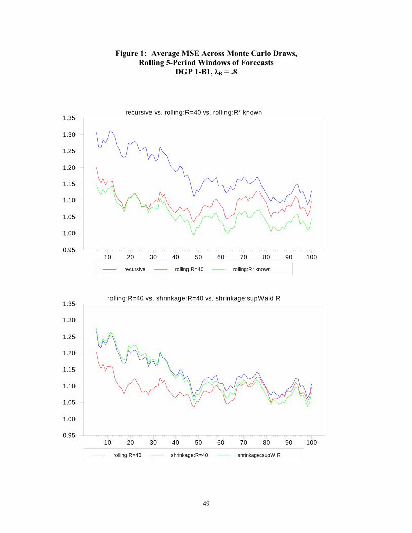
49
Figure 1: Average MSE Across Monte Carlo Draws, Rolling 5-Period Windows of Forecasts
DGP 1-B1, λB = .8
recursive rolling:R=40 rolling:R* known
recursive vs. rolling:R=40 vs. rolling:R* known
10 20 30 40 50 60 70 80 90 1000.95
1.00
1.05
1.10
1.15
1.20
1.25
1.30
1.35
rolling:R=40 shrinkage:R=40 shrinkage:supW R
rolling:R=40 vs. shrinkage:R=40 vs. shrinkage:supWald R
10 20 30 40 50 60 70 80 90 1000.95
1.00
1.05
1.10
1.15
1.20
1.25
1.30
1.35