improving markov network structure learning using - lirias

Journal of Machine Learning Research 1 (2012) 1-48 Submitted 9/12; Published ?/??

Improving Markov Network Structure Learning UsingDecision Trees

Daniel Lowd [email protected] of Computer and Information ScienceUniversity of OregonEugene, OR 97403, USA

Jesse Davis [email protected]

Department of Computer Science

Katholieke Universiteit Leuven

3001 Heverlee, Belgium

Editor: ??

Abstract

Most existing algorithms for learning Markov network structure either are limited tolearning interactions among few variables or are very slow, due to the large space of possiblestructures. In this paper, we propose three new methods for using decision trees to learnMarkov network structures. The advantage of using decision trees is that they are veryfast to learn and can represent complex interactions among many variables. The firstmethod, DTSL, learns a decision tree to predict each variable and converts each tree intoa set of conjunctive features that define the Markov network structure. The second, DT-BLM, builds on DTSL by using it to initialize a search-based Markov network learningalgorithm recently proposed by Davis and Domingos (2010). The third, DT+L1, combinesthe features learned by DTSL with those learned by an L1-regularized logistic regressionmethod (L1) proposed by Ravikumar et al. (2009). In an extensive empirical evaluationon 20 datasets, DTSL is comparable to L1 and significantly faster and more accurate thantwo other baselines. DT-BLM is slower than DTSL, but obtains slightly higher accuracy.DT+L1 combines the strengths of DTSL and L1 to perform significantly better than eitherof them with only a modest increase in training time.

Keywords: Markov networks, structure learning, decision trees, probabilistic methods

1. Introduction

A Markov network is an undirected, probabilistic graphical model for compactly represent-ing a joint probability distribution over a set of random variables. In general, these variablescan be discrete, continuous, or a mix; in this paper, we consider the case when all variablesare discrete. Markov networks have been widely used in a number of domains, includingcomputer vision, computational biology, and natural language processing. The structureof a Markov network defines which direct interactions among the variables are includedin the model. This structure can be represented as a set of features, each of which is aBoolean-valued function of a subset of the variables. The parameters of a Markov networkdefine the relative strength of those interactions. Selecting a Markov network structure that

c©2012 Daniel Lowd and Jesse Davis.

Lowd and Davis

includes the most important interactions in a domain is therefore essential for building anaccurate model of that domain.

For some tasks, such as image processing, the structure of the Markov network may behand crafted to fit the problem. In other problems, the structure is unknown and must belearned from data. These learned structures may be interesting in themselves, since theyshow the most significant direct interactions in the domain. In many domains, however, thegoal is not an interpretable structure but an accurate final model. It is this last scenariothat is the focus of our paper: learning the structure of a Markov network in order toaccurately estimate marginal and conditional probabilities.

Learning an effective structure is difficult due to the very large structure space—thenumber of possible sets of conjunctive features is doubly-exponential in the number ofvariables. As a result, most previous approaches to learning Markov network structureare either very slow or limited to relatively simple features, such as only allowing pairwiseinteractions. In this paper, we propose to overcome these limitations by using decision treelearners, which are able to quickly learn complex structures involving many variables.

Our first method, DTSL (Decision Tree Structure Learner), learns probabilistic decisiontrees to predict the value of each variable and then converts the trees into sets of conjunctivefeatures. We propose and evaluate several different methods for performing the conversion.Finally, DTSL merges all learned features into a global model. Weights for these featurescan be learned using any standard Markov network weight learning method. DTSL issimilar in spirit to work by Ravikumar et al. (2010), who learn a sparse logistic regressionmodel for each variable and combine the features from each local model into a global networkstructure. DTSL can also be viewed as converting a dependency network (Heckerman et al.,2000) with decision trees into a consistent Markov network.

Our second method, DT-BLM (Decision Tree Bottom-Up Learning), builds on DTSLby using the BLM algorithm of Davis and Domingos (2010) to further refine the structurelearned by DTSL. This algorithm is much slower, but usually more accurate than DTSL.Furthermore, it serves as an example of how decision trees can be used to improve search-based structure learning algorithms by providing a good initial structure.

Our third method, DT+L1, combines the structure learned by DTSL with the pairwiseinteractions learned by L1-regularized logistic regression (L1) (Ravikumar et al., 2010).The trees used by DTSL are good at capturing higher-order interactions, but each leaf ismutually exclusive. In contrast, L1 captures many independent interaction terms, but eachinteraction is between just two variables. Their combination offers the potential to representboth kinds of interaction, leading to better performance in many domains.

We conducted an extensive empirical evaluation on 20 real-world datasets. We foundthat DTSL offers similar accuracy and speed as L1, performing better on datasets where itfinds interesting tree structure and worse on datasets where it does not. Over 90% of therunning time was spent learning weights, so there is potential to improve learning times evenmore with more sophisticated weight learning algorithms. The hybrid DT-BLM algorithmis often more accurate than DTSL, but is also much slower due to the additional refinementstep. DT+L1 often has the best overall accuracy and runs much faster than DT-BLM,making it a very good algorithm overall. We also evaluated two other baseline structurelearners, but they were not competitive with L1 and the three variants of DTSL.

2

Improving Markov Network Structure Learning Using Decision Trees

This journal paper is an extended and improved version of the conference paper (Lowdand Davis, 2010). The extensions include two additional algorithms (DT-BLM and DT+L1)and more extensive experiments, including seven additional datasets and learning curves.The presentation has also been expanded and polished.

2. Markov Networks

This section provides a basic overview about Markov networks.

2.1 Representation

A Markov network is a model for the joint probability distribution of a set of variablesX = (X1, X2, . . . , Xn) (Della Pietra et al., 1997). It is often expressed as an undirectedgraph G and a set of potential functions φk. The graph has a node for each variable, andthe model has a potential function for each clique in the graph. The joint distributionrepresented by a Markov network is:

P (X=x) =1

Z

∏k

φk(x{k}) (1)

where x{k} is the state of the variables that appear in the kth clique, and Z is a normalizationconstant called the partition function.

The graph encodes the following conditional independencies: sets of variables XA andXB are conditionally independent given evidence Y if all paths between their correspondingnodes in the graph pass through nodes from Y. Any probability distribution that canbe represented as a product of potential functions over the cliques of the graph, as inEquation (1), satisfies these independencies; for positive distributions, the converse holdsas well.

One of the limitations of the graph structure is that it says nothing about the structureof the potential functions themselves. The most standard representation of a potentialfunction over discrete variables is a table with one value for each variable configuration, butthis requires a number of parameters that is exponential in the size of the clique. To learnan effective probability distribution, we typically need a finer-grained parametrization thatpermits a compact distribution even when the cliques are relatively large.

Therefore, we focus on learning the log-linear representation of a Markov network, inwhich the clique potentials are replaced by an exponentiated weighted sum of features ofthe state:

P (X=x) =1

Zexp

∑j

wjfj(x{j})

(2)

A feature fj(x{j}) may be any real-valued function of the state. For discrete data, a featuretypically is a conjunction of tests of the form Xi = xi, where Xi is a variable and xi isa value of that variable. We say that a feature matches an example if it is true of thatexample. Any positive probability distribution over a discrete domain can be representedas log-linear model with conjunctive features. For example, a product of tabular potentialfunctions could be converted into a log-linear model by constructing one conjunctive featurefor each row of each table, using the log of the potential function value as the feature weight.

3

Lowd and Davis

In this paper, we will refer to this set of conjunctive features as the structure of theMarkov network. This detailed structure specifies not only the independencies of the dis-tribution, but also the specific interaction terms that are most significant. If desired, thesimpler undirected graph structure can be constructed from the features by adding an edgebetween each pair of nodes whose variables appear together in a feature.

2.2 Inference

The main inference task in graphical models is to compute the conditional probability ofsome variables (the query) given the values of some others (the evidence), by summing outthe remaining variables. This problem is #P-complete. Thus, approximate inference tech-niques are required. One widely used method is Markov chain Monte Carlo (MCMC) (Gilkset al., 1996), and in particular Gibbs sampling, which proceeds by sampling each variablein turn given its Markov blanket, the variables it appears with in some potential or feature.These samples can be used to answer probabilistic queries by counting the number of sam-ples that satisfy each query and dividing by the total number of samples. Under modestassumptions, the distribution represented by these samples will eventually converge to thetrue distribution. However, convergence may require a very large number of samples, anddetecting convergence is difficult.

2.3 Weight Learning

The goal of weight learning is to select feature weights that maximize a given objectivefunction. One of the most popular objective functions is the log-likelihood of the trainingdata. In a Markov network, the negative log-likelihood is a convex function of the weights,and thus weight learning can be posed as a convex optimization problem. However, this op-timization typically requires evaluating the log-likelihood and its gradient in each iteration.This is typically intractable to compute exactly due to the partition function. Further-more, an approximation may work poorly: Kulesza and Pereira (2007) have shown thatapproximate inference can mislead weight learning algorithms.

A more computationally efficient alternative, widely used in areas such as spatial statis-tics, social network modeling, and language processing, is to optimize the pseudo-likelihoodor pseudo-log-likelihood (PLL) instead (Besag, 1975). Pseudo-likelihood is the product ofthe conditional probabilities of each variable given its Markov blanket; pseudo-log-likelihoodis the log of the pseudo-likelihood:

logP •w(X=x) =V∑j=1

N∑i=1

logPw(Xi,j =xi,j |MBx(Xi,j)) (3)

where V is the number of variables, N is the number of examples, xi,j is the value of the jthvariable of the ith example, MBx(Xi,j) is the state of Xi,j ’s Markov blanket in the data.PLL and its gradient can be computed efficiently and optimized using any standard convexoptimization algorithm, since the negative PLL of a Markov network is also convex.

4


3. Structure Learning in Markov Networks

Our goal in structure learning is to find a succinct set of features that can be used toaccurately represent a probability distribution in a domain of interest. Other goals includelearning the independencies or causal structure in the domain, but we focus on accurateprobabilities. In this section, we briefly review four categories of approaches for Markovnetwork structure learning, along with their strengths and weaknesses.

Global Search-Based Learning. One of the common approaches is to perform aglobal search for a set of features that accurately captures high-probability regions of theinstance space (Della Pietra et al., 1997; McCallum, 2003). The algorithm of Della Pietraet al. (1997) is the most canonical example of this approach. The algorithm starts witha set of atomic features, each consisting of one state of one variable. It creates candidatefeatures by conjoining each feature to each other feature, including the original atomicfeatures. It calculates the weight for each candidate feature by assuming that all otherfeature weights remain unchanged, which is done for efficiency reasons. It uses Gibbssampling for inference when setting the weight. Then, it evaluates each candidate feature fby estimating how much adding f would increase the log-likelihood. It adds the feature thatresults in the largest gain to the feature set. This procedure terminates when no candidatefeature improves the model’s score.

Recently, Davis and Domingos (2010) proposed an alternative bottom-up approach,called Bottom-up Learning of Markov Networks (BLM), for learning the structure of aMarkov network. BLM starts by treating each complete example as a long feature in theMarkov network. The algorithm repeatedly iterates through the feature set. It considersgeneralizing each feature to match its k nearest previously unmatched examples by droppingvariables. If incorporating the newly generalized feature improves the model’s score, it isretained in the model. The process terminates when no generalization improves the score.

These discrete search approaches are often slow due to the exponential number of pos-sible features, leading to a doubly-exponential space of possible structures. Even a greedysearch through this space must use the training data to repeatedly evaluate many candi-dates.

Optimization-Based Learning. Instead of performing a discrete search through pos-sible structures, other recent work has framed the search as a continuous weight optimiza-tion problem with L1 regularization for sparsity (Lee et al., 2007; Schmidt and Murphy,2010). The final structure consists of all features that are assigned non-zero weights. Thesemethods are somewhat more efficient, but are typically limited to relatively short features.For example, in the approach of Lee et al. (2007), the set of candidate features must bespecified in advance, and must be small enough that the gradient of all feature weights canbe computed. Even including interactions among three variables requires a cubic numberof features. Learning higher-order interactions quickly becomes infeasible. Schmidt andMurphy (2010) propose an algorithm that can learn longer features, as long as they satisfya hierarchical constraint: longer features are only included when all subsets of the featurehave been assigned non-zero weights. In experiments, this method does identify some longerfeatures, but most features are short.

Independence Test Based Learning. Another line of work attempts to identify theMarkov network structure directly by performing independence tests (Spirtes et al., 1993).

5

Lowd and Davis

The basic idea is that if two variables are conditionally independent given some othervariables then there should be no edge between them in the Markov network. Thus, insteadof searching for interactions among the variables, these methods search for independencies.The challenge is the large number of conditional independencies to test: simply testing formarginal independence among each pair of variables is quadratic in the number of variables,and the complexity grows exponentially with the size of the separating set. Some variantsof this approach search for the Markov blanket of each variable, the minimal set of variablesthat renders it conditionally independent from all others (Bromberg et al., 2009). Usingindependencies in the data to infer additional independencies can speed up this search, butmany tests are still required. Furthermore, reliably recovering the independencies may notnecessarily lead to the most accurate probabilistic model, since that is not the primary goalof these methods.

Learning Local Models. Ravikumar et al. (2010) proposed the alternative idea oflearning a local model for each variable and then combining these models into a globalmodel. Their method learns the structure by trying to discover the Markov blanket ofeach variable. It considers each variable Xi in turn and builds an L1-regularized logisticregression model to predict the value of Xi given the remaining variables. L1 regularizationencourages sparsity, so that most of the variables end up with a weight of zero. TheMarkov blanket of Xi is all variables that have non-zero weight in the logistic regressionmodel. Under certain conditions, this is a consistent estimator of the structure of a pairwiseMarkov network. In practice, when learned from real-world data, these Markov blankets areoften incompatible with each other; for example, Xi may be in the inferred Markov blanketof Xj while the reverse does not hold. There are two methods for resolving these conflicts.One is to include an edge if either Xi is in Xj ’s Markov blanket or Xj is in Xi’s Markovblanket. The other method is to include an edge only if Xi is in Xj ’s Markov blanketand Xj is in Xi’s Markov blanket. In the final model, if there is an edge between Xi andXj then the log-linear model includes a pairwise feature involving those two variables. Allweights are then learned globally using any standard weight learning algorithm. While thisapproach greatly improves the tractability of structure learning, it is limited to modelingpairwise interactions, ignoring all higher-order effects. Furthermore, it still exhibits longrun times for domains that have large numbers of variables.

4. Decision Tree Structure Learning (DTSL)

We now describe our method for learning Markov network structure from data, decisiontree structure learning (DTSL). Algorithm 1 outlines our basic approach. For each variableXi, we learn a probabilistic decision tree to represent the conditional probability of Xi givenall other variables, P (Xi|X − Xi). Each tree is converted to a set of conjunctive featurescapable of representing the same probability distribution as the tree. Finally, all featuresare taken together in a single model and weights are learned globally using any standardweight learning algorithm.

This is similar in spirit to learning a dependency network (Heckerman et al., 2000): Bothdependency networks (with tree distributions) and DTSL learn a probabilistic decisiontree for each variable and combine the trees to form a probabilistic model. However, adependency network may not represent a consistent probability distribution, and inference

6


!"#$%"#&'( !"#)%"#*'( !"#*%"#)'(

+$(

+,(

-.+)/+$%+,0(((1(

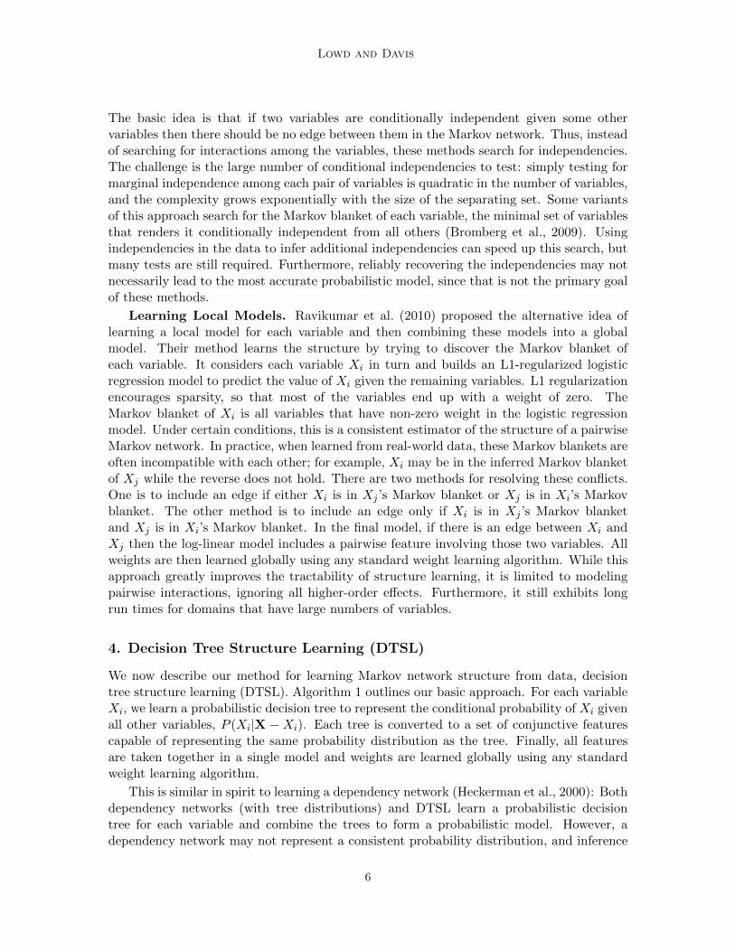
Figure 1: Example of a probabilistic decision tree.

can only be done by Gibbs sampling. In contrast, the Markov networks learned by DTSLalways represent consistent probability distributions and allow inference to be done by anystandard technique, such as loopy belief propagation (Murphy et al., 1999), mean field, orMCMC.

We now describe each step of DTSL in more detail.

Algorithm 1 The DTSL Algorithm

function DTSL(training examples D, variables X)F ← ∅for all Xi ∈X doTi ← LearnTree(D,Xi)Fi ← GenerateFeatures(Ti)F ← F ∪ Fi

end forM ←LearnWeights(F,D)return M

4.1 Learning Trees

A probabilistic decision tree represents a probability distribution over a target variable, Xi,given a set of inputs. Each interior node tests the value of an input variable and each of itsoutgoing edges is labeled with one of the outcomes of that test (e.g., true or false). Each leafnode contains the conditional distribution (e.g., multinomial) of the target variable giventhe test outcomes specified by its ancestor nodes and edges in the tree. We focus on discretevariables and consider tests of the form Xj = xj , where Xj is a variable and xj is valueof that variable. Each conditional distribution is represented by a multinomial. Figure 1contains an example of a probabilistic decision tree.

We can learn a probabilistic decision tree from data in a depth-first manner, one splitat a time. We select a split at the root, partition the training data into the sets matchingeach outgoing branch, and recurse. We select each split to maximize the conditional log-likelihood of the target variable. This is very similar to using information gain as the splitcriterion. We used multinomials as the leaf distributions with a Dirichlet prior (α = 1)for smoothing. In order to help avoid overfitting, we used a structure prior P (S) ∝ κp,

7

Lowd and Davis

where p is the number of parameters and κ < 1 represents a multiplicative penalty foreach additional parameter in the model, as in Chickering et al. (1997). To further avoidoverfitting, we set the minimum number of examples at each leaf to 10. Any splits thatwould result in fewer examples in a leaf are rejected.

Pseudocode for the tree learning subroutine is in Algorithm 2.

Algorithm 2 DTSL Tree Learning Subroutine

function LearnTree(training examples D, variable Xi)best split← ∅best score← 0for all Xj ∈X −Xi dofor all xj ∈ Val(Xj) doS ← (Xj = xj)if Score(S,Xi, D) > best score then

best split ← Sbest score ←Score(S,Xi, D)

end ifend for

end forif best score > log κ then

(Dt, Df )←SplitData(D, best split)TL ←LearnTree(Dt, Xi)TR ←LearnTree(Df , Xi)return new TreeVertex(best split, TL, TR)

elseUse D to estimate P (Xi)return new TreeLeaf(P (Xi))

end if

4.2 Generating Features

While decision trees are not commonly thought of as a log-linear model, any decision tree canbe converted to a set of conjunctive features. In addition to a direct translation (Default),we explored four modifications (Prune, Prune-10, Prune-5, and Nonzero) which couldyield structures with easier weight learning or better generalization.

The Default feature generation method is a direct translation of a probabilistic decisiontree to an equivalent set of features. For each state of the target variable, we generate afeature for each path from the root to a leaf. The feature’s conditions specify a single stateof the target variable and all variable tests along the path in the decision tree. For example,to convert the decision tree in Figure 1 to a set of rules, we generate two features for eachleaf, one where X4 is true and one where X4 is false. The complete list of features is asfollows:

1. X1 = T ∧X4 = T

2. X1 = T ∧X4 = F

8


3. X1 = F ∧X2 = T ∧X4 = T

4. X1 = F ∧X2 = T ∧X4 = F

5. X1 = F ∧X2 = F ∧X4 = T

6. X1 = F ∧X2 = F ∧X4 = F

By using the log probability at the leaf as the rule’s weight, we obtain a log linear modelrepresenting the same distribution. By applying this transformation to all decision trees,we obtain a set of conjunctive features that comprise the structure of our Markov network.However, their weights may be poorly calibrated (e.g., due to the same feature appearingin several decision trees), so weight learning is still necessary.

The Prune method expands the set of features generated by Default in order to makelearning and inference easier. One disadvantage of the Default procedure is that it gener-ates very long features with many conditions when the source trees are deep. Intuitively, wewould like to capture the coarse interactions with short features and the finer interactionswith longer features, rather than representing everything with long features. In the Prunemethod, we generate additional features for each path from the root to an interior node,not just paths from the root to a leaf. Each feature’s conditions specify a single state ofthe target variable and all variable tests along the path in the decision tree. However, weinclude paths ending at any node, not just at leaves.

Specifically, for each state of the target variable and node in the tree (leaf or non-leaf), we generate a feature that specifies the state of the target variable and contains acondition for each ancestor of the node. This is equivalent to applying the Default featuregeneration method to all possible “pruned” versions of a decision tree, that is, where one ormore interior nodes are replaced with leaves. This yields four additional rules, in additionto those enumerated above:

1. X4 = T

2. X4 = F

3. X1 = F ∧X4 = T

4. X1 = F ∧X4 = F

The Prune-10 and Prune-5 methods begin with the features generated by Prune andremove all features with more than 10 and 5 conditions, respectively. This can help avoidoverfitting.

Our final feature generation method, Nonzero, is similar to Default, but removesall false variable constraints in a post-processing step. For example, the decision tree inFigure 1 would be converted to the following set of rules:

1. X1 = T ∧X4 = T

2. X1 = T

3. X2 = T ∧X4 = T

4. X2 = T

5. X4 = T

This simplification is designed for sparse binary domains such as text, where a value of falseor zero contains much less information than a value of true or one.

9

Lowd and Davis

4.3 Asymptotic Complexity

Next, we explore DTSL’s efficiency by analyzing its asymptotic complexity. Let n be thenumber of variables, m be the number of training examples, and l be the number of valuesper variable. The complexity of selecting the first split is O(lmn), since we must computestatistics for each of the l values of each of the n variables using all of the m examples. Atthe next level, we now have two splits to select: one for the left child and one for the rightchild of the original split. However, since the split partitions the training data into two sets,each of the m examples is only considered once, either for the left split or the right split,leading to a total time of O(lmn) at each level. If each split assigns a fraction of at least 1/kexamples to each child, then the depth is at most O(logk(m)), yielding a total complexityof O(lmn logk(m)) for one tree, and O(lmn2 logk(m)) for the entire structure. Dependingon the patterns present in the data, the depth of the learned trees could be much less thanlogk(m), leading to faster run times in practice. For large datasets or streaming data, wecan apply the Hoeffding tree algorithm, which uses the Hoeffding bound to select decisiontree splits after enough data has been seen to make a confident choice, rather than usingall available data (Domingos and Hulten, 2000).

5. Decision Tree Bottom-Up Learning (DT-BLM)

The DTSL algorithm works by first using a decision tree learner to generate a set of con-junctive features and then learning weights for those features. In this section, we proposeusing decision trees within the context of the BLM Markov network structure learningalgorithm (Davis and Domingos, 2010), which is described in Section 3.

BLM starts with a large set of long (i.e., specific) features and simplifies them to makethem more general. The standard BLM algorithm uses the set of all training examplesas the initial feature set. However, BLM could, in principle, generalize any set of initialfeatures. The key idea of DT-BLM is to run BLM on the features from DTSL.

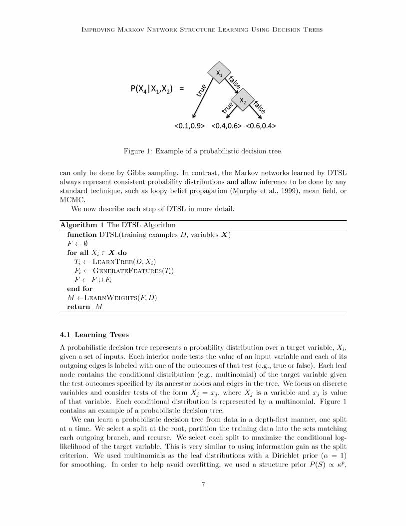
Algorithm 3 outlines the DT-BLM algorithm. DT-BLM receives a set of training exam-ples, D, a set of variables, X, and a set of integers, K, as input. It begins by running DTSL.Of the five feature conversion methods, it selects whichever one results in the best scoringmodel on validation data. Then DT-BLM employs the standard BLM learning procedure,but uses the features learned by DTSL as the initial feature set. The main loop in BLMinvolves repeatedly iterating through the feature set, calling the GeneralizeFeaturemethod on each feature f in the feature set F .

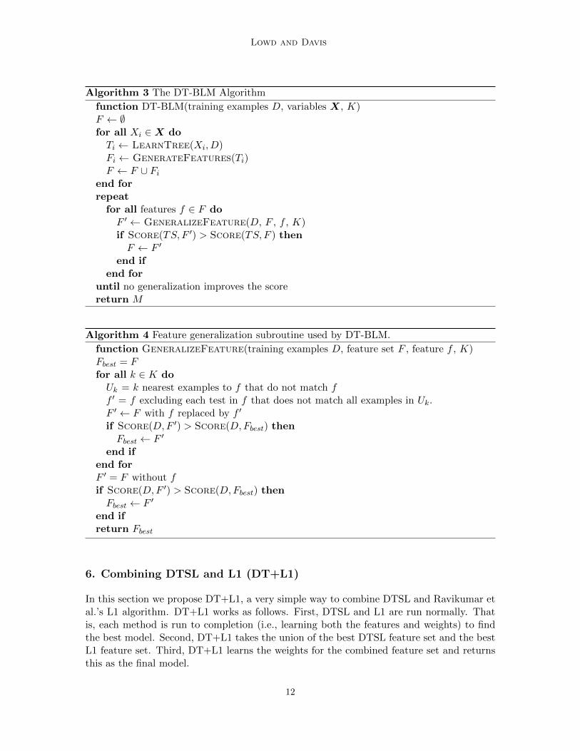
The GeneralizeFeature method, outlined in Algorithm 4, proposes and scores severalcandidate feature generalizations. Specifically, it creates one generalization, f ′, for eachk ∈ K by finding the set of examples Uk which are f ’s k nearest unmatched examples. Next,it creates f ′ by dropping each variable-value test in f that does not match all examples inUk, which has the effect of generalizing f ′ to match all examples in this set. It also scoresthe effect of removing f from F .

DT-BLM measures the distance between a feature and an example using the generalizedvalue difference metric (GVDM), which tends to perform better in practice than the simpler

10


Hamming distance (Davis and Domingos, 2010). Formally, the distance, D(f, e) is:

D(f, e) =∑c∈f

GVDM(f, e, c) (4)

where f is a feature, e is an example, c ranges over the variables in f and

GVDM(f, e, c) =∑h

∑fi∈f,fi 6=c

|P (c = h|fi)− P (c = h|efi)|Q

where h ranges over the possible values of variable c, fi is the value of the ith variable inf , efi is the value of the attribute referenced by fi in e, and Q is an integer. For a variablec that appears in f , GVDM measures how well the other variables in f predict c. Theintuition is that if c appears in a feature then the other variables should be good predictorsof c.

Each generalization is evaluated by replacing f with the generalization in the model,relearning the weights of the modified feature set, and scoring the new model as:

S(D,F ′, α) = PLL(D,F ′)− α∑fi∈F ′

|fi| (5)

where PLL(D,F ′) is the train set pseudo-likelihood of feature set F ′, α is a penalty term toavoid overfitting, and |fi| is the number of variable-value tests in feature fi. The procedurereturns the best scoring generalized feature set, F ′. DT-BLM updates F to F ′ if F ′ has abetter score. The process terminates after making one full loop over the feature set withoutchanging F by accepting a generalization.

The advantage of DT-BLM over DTSL is that it can refine individual features based ontheir global contribution to the pseudo-likelihood. This can lead to simpler models in termsof both the number and length of the features. One advantage of DT-BLM over BLM isthat the features selected by DTSL are already very effective, so BLM is less likely to endup in a bad local optimum. A second advantage is that it removes the restriction that BLMcan never learn a model that has more features than examples. This is valuable for domainswhich are most effectively modeled with a large number of short features (e.g., text). Theprinciple disadvantage of DT-BLM is speed: it can be much slower than DTSL, since it isdoing a secondary search over feature simplifications. We have also found that DT-BLMis sensitive to the Gaussian weight prior used during the BLM structure search, unlike thestandard BLM algorithm. This means that DT-BLM requires more tuning time than BLM,as discussed more extensively in our empirical evaluation in Section 7.

Note that DT-BLM is similar in spirit to Bayesian network structure learning algorithmsthat combine independence-test and search-based learning techniques (Tsamardinos et al.,2006). These algorithms work in two phases. In the first step, they identify a superset ofthe edges that could be included in the network using independence tests. In the secondstep, a search through the space of possible structures is performed, but it is restrictedto only consider including candidate edges identified in the first step. Typically, a greedy,general-to-specific search is employed. These algorithms differ from DT-BLM in three keyways: DT-BLM searches for features and not edges; DT-BLM uses decision trees to identifycandidate features and not independence tests; and DT-BLM uses a specific-to-generalsearch and not a general-to-specific search to refine the structure.

11

Lowd and Davis

Algorithm 3 The DT-BLM Algorithm

function DT-BLM(training examples D, variables X, K)F ← ∅for all Xi ∈X doTi ← LearnTree(Xi, D)Fi ← GenerateFeatures(Ti)F ← F ∪ Fi

end forrepeat

for all features f ∈ F doF ′ ← GeneralizeFeature(D, F , f , K)if Score(TS, F ′) > Score(TS, F ) thenF ← F ′

end ifend for

until no generalization improves the scorereturn M

Algorithm 4 Feature generalization subroutine used by DT-BLM.

function GeneralizeFeature(training examples D, feature set F , feature f , K)Fbest = Ffor all k ∈ K doUk = k nearest examples to f that do not match ff ′ = f excluding each test in f that does not match all examples in Uk.F ′ ← F with f replaced by f ′

if Score(D,F ′) > Score(D,Fbest) thenFbest ← F ′

end ifend forF ′ = F without fif Score(D,F ′) > Score(D,Fbest) thenFbest ← F ′

end ifreturn Fbest

6. Combining DTSL and L1 (DT+L1)

In this section we propose DT+L1, a very simple way to combine DTSL and Ravikumar etal.’s L1 algorithm. DT+L1 works as follows. First, DTSL and L1 are run normally. Thatis, each method is run to completion (i.e., learning both the features and weights) to findthe best model. Second, DT+L1 takes the union of the best DTSL feature set and the bestL1 feature set. Third, DT+L1 learns the weights for the combined feature set and returnsthis as the final model.

12


The advantage of this approach is that it combines the strengths of both algorithms.DTSL excels at learning long features that capture complex interactions. Ravikumar et al.’sL1 approach only learns pairwise features, which occur less frequently in DTSL’s learnedmodels. One disadvantage is that DT+L1 will be more time intensive than either approachindependently. DT+L1 involves performing parameter tuning to select the best model forboth DTSL and L1 and then another run of weight learning, including parameter tuning,on the combined feature set. Another potential problem is that the combined model willhave more features, which may lead to a more complex inference task.

7. Empirical Evaluation

We evaluate our algorithms on 20 real-world datasets. The goals of our experiments arethree-fold. First, we want to determine how the different feature generation methods affectthe performance of DTSL and DT-BLM (Section 7.3). Second, we want to compare theaccuracy of DTSL, DT-BLM, and DT+L1 to each other as well as to several state-of-the-art Markov network structure learners: the algorithm of Della Pietra et al. (1997), whichwe refer to as DP; BLM (Davis and Domingos, 2010); and L1-regularized logistic regres-sion (Ravikumar et al., 2010) (Section 7.4). Finally, we want to compare the running timeof these learning algorithms, since this greatly affects their practical utility (Section 7.5).

7.1 Methodology

We used DTSL, DT-BLM, DT+L1, and each of the baselines to learn structures on 20datasets.

DTSL was implemented in OCaml. For both BLM and DP, we used the publicly avail-able code of Davis and Domingos (2010). Since DT-BLM is built on both DTSL and BLM,it used a combination of the DTSL and BLM code as well. For Ravikumar et al.’s ap-proach, we tried both the OWL-QN (Andrew and Gao, 2007) and LIBLINEAR (Fan et al.,2008) software packages. Our initial experiments and evaluation were done using OWL-QN,but we later discovered that LIBLINEAR was much faster with nearly identical accuracy.Therefore, to be as fair as possible to L1, we report the running times for LIBLINEAR.

The output of each structure learning algorithm is a set of conjunctive features. Tolearn weights, we optimized the pseudo-likelihood of the data via the limited-memory BFGSalgorithm (Liu and Nocedal, 1989) since optimizing the likelihood of the data is prohibitivelyexpensive for the domains we consider.

Like Lee et al. (2007), we evaluated our algorithm using test set conditional marginallog-likelihood (CMLL). To make results from different datasets more comparable, we reportnormalized CMLL (NCMLL), which is CMLL divided by the number of variables in thedomain. Calculating the NCMLL requires dividing the variables into a query set Q and anevidence set E. Then, for each test example we computed:

NCMLL(X = x) =1

|X|∑i∈Q

logP (Xi = xi|E)

For each domain, we divided the variables into four disjoint sets. One set served as the queryvariables while the remaining three sets served as evidence. We repeated this procedure so

13

Lowd and Davis

that each set served as the query variables once. We computed the conditional marginalprobabilities using Gibbs sampling, as implemented in the open-source Libra toolkit.1 Forall domains, we ran 10 independent chains, each with 100 burn-in samples and followedby 1,000 samples for computing the probability. CMLL is related to PLL (Equation 3),since both measure the ability of the model to predict individual variables given evidence.However, we used approximately 75% of the variables as evidence when computing CMLL,while PLL always uses all-but-one variable as evidence.

We tuned all algorithms using separate validation sets, the same validation sets usedby Haaren and Davis (2012). For DTSL, we selected the structure prior κ for each domainthat maximized the total log-likelihood of all probabilistic decision trees on the validationset. The values of κ we used were powers of 10, ranging from 0.0001 to 1.0. When learningthe weights for each feature generation method, we placed a Gaussian prior with mean 0on each feature weight and then tuned the standard deviation to maximize PLL on thevalidation set, with values of 100, 10, 1, and 0.1. For comparisons to other algorithms, weselected the DTSL model with the best pseudo-likelihood on the validation set. We choseto use pseudo-likelihood for tuning instead of CMLL because it is much more efficient tocompute.

For L1, on each dataset we tried the following values of the LIBLINEAR tuning param-eter C: 0.001, 0.01, 0.05, 0.1, 0.5, 1 and 5.2 We also tried both methods of making theMarkov blankets consistent. These parameter settings allowed us to explore a variety ofdifferent models, ranging from those containing all pairwise interactions to those that werevery sparse. We also tuned the weight prior as we did with DTSL. Tuning the standarddeviation of the Gaussian weight prior allowed us to get better results than reported byDavis and Domingos (2010).

For BLM and DP, we kept the tuning settings used by Davis and Domingos (2010).We tried performing additional tuning of the weight prior for BLM, but it did not lead toimproved results. For DT+L1, we combined the DTSL and L1 structures and relearned thefinal weights, including tuning the Gaussian weight prior on the validation set.

All of our code is available at http://ix.cs.uoregon.edu/~lowd/dtsl under a modi-fied BSD license.

7.2 Datasets

For our experiments, we used the same set of 20 domains as Haaren and Davis (2012), 13of which were previously used by Davis and Domingos (2010).3 All variables are binary-valued. Basic statistics for all datasets are in Table 1, ordered by number of variables in thedomain. “Density” refers to the fraction of non-zero entries. Below, we provide additionalinformation about each dataset.

We used four clickstream prediction domains: KDDCup 2000, MSNBC, AnonymousMSWeb,4 and Kosarek.5 Each data point was a single session, with one binary-valued

1. Available from http://libra.cs.uoregon.edu/.2. C is the inverse of the L1 regularization weight λ used by OWL-QN (Andrew and Gao, 2007). Larger C

values almost always resulted in generating all pairwise features.3. Publicly available at http://alchemy.cs.washington.edu/papers/davis10a4. Available from the UCI machine learning repository (Blake and Merz, 2000).5. http://fimi.ua.ac.be/data/

14


Dataset # Train Ex. # Tune Ex. # Test Ex. # Vars Density

1. NLTCS 16,181 2,157 3,236 16 0.3322. MSNBC 291,326 38,843 58,265 17 0.1663. KDDCup 2000 180,092 19,907 34,955 64 0.0084. Plants 17,412 2,321 3,482 69 0.1805. Audio 15,000 2,000 3,000 100 0.1996. Jester 9,000 1,000 4,116 100 0.6087. Netflix 15,000 2,000 3,000 100 0.5418. Accidents 12,758 1,700 2,551 111 0.2919. Retail 22,041 2,938 4,408 135 0.02410. Pumsb Star 12,262 1,635 2,452 163 0.27011. DNA 1,600 400 1,186 180 0.25312. Kosarek 33,375 4,450 6,675 190 0.02013. MSWeb 29,441 3,270 5,000 294 0.01014. Book 8,700 1,159 1,739 500 0.01615. EachMovie 4,524 1,002 591 500 0.05916. WebKB 2,803 558 838 839 0.06417. Reuters-52 6,532 1,028 1,540 889 0.03618. 20 Newsgroups 11,293 3,764 3,764 910 0.04919. BBC 1,670 225 330 1,058 0.07820. Ad 2,461 327 491 1,556 0.008

Table 1: Dataset characteristics.

variable for each page, area, or category of the site, indicating if it was visited during thatsession or not. For KDD Cup 2000 (Kohavi et al., 2000), we used the subset of Hultenand Domingos (2002), which consisted of 65 page categories. We dropped one categorythat was never visited in the training data. The MSNBC anonymous web data containsinformation about which top-level MSNBC pages were visited during a single session. TheMSWeb anonymous web data contains visit data for 294 areas (Vroots) of the Microsoftweb site, collected during one week in February 1998. Kosarek is clickstream data from aHungarian online news portal.

Five of our domains were from recommender systems: Audio, Book, EachMovie, Jesterand Netflix. The Audio dataset consists of information about how often a user listened toa particular artist.6 The data was provided by the company Audioscrobbler before it wasacquired by Last.fm. We focused on the 100 most listened-to artists. We used a randomsubset of the data and reduced the problem to “listened to” or “did not listen to.” TheBook Crossing (Book) dataset (Ziegler et al., 2005) consists of a user’s rating of how muchthey liked a book. We considered the 500 most frequently rated books. We reduced theproblem to “rated” or “not rated” and considered all people who rated at least two of thesebooks. EachMovie7 is a collaborative filtering dataset in which users rate movies they haveseen. We focused on the 500 most-rated movies, and reduced each variable to “rated” or

6. http://www-etud.iro.umontreal.ca/~bergstrj/audioscrobbler_data.html7. Provided by Compaq at http://research.compaq.com/SRC/eachmovie/; no longer available for down-

load, as of October 2004.

15

Lowd and Davis

“not rated”. The Jester dataset (Goldberg et al., 2001) consists of users’ real-valued ratingsfor 100 jokes. For Jester, we selected all users who had rated all 100 jokes, and reducedtheir preferences to “like” and “dislike” by thresholding the real-valued preference ratingsat zero. Finally, we considered a random subset of the Netflix challenge data and focused onthe 100 most frequently rated movies. We reduced the problem to “rated” or “not rated.”

We used four text domains: 20 Newsgroups, Reuters-52, WebKB8, and BBC9. For20 Newsgroups, we only considered words that appeared in at least 200 documents. ForReuters, WebKB, and BBC, we only considered words that appeared in at least 50 docu-ments. For all four datasets, we created one binary feature for each word. The text domainscontained roughly a 50-50 train-test split, whereas all other domains used around 75% ofthe data for the training, 10% for tuning, and 15% for testing. Thus we split the test setof these domains to make the proportion of data devoted to each task more closely matchthe other domains used in the empirical evaluation.

The remaining seven datasets have no unifying theme. Plants consists of different planttypes and locations where they are found.4 We constructed one binary feature for eachlocation, which is true if the plant is found there. DNA10 is DNA sequences for primatesplice-junctions; we used the binary-valued encoding provided. The National Long TermCare Survey (NLTCS) data consist of binary variables that measure an individual’s abilityto perform different daily living activities.11 Pumsb Star contains census data for populationand housing.5 Accidents contains anonymized traffic incident data.5 Retail is market basketdata from a Belgian retail store.5

7.3 Feature Generation Methods

First, we compared the accuracy of DTSL with different feature generation methods: De-fault, Prune, Prune-10, Prune-5, and Nonzero. Table 2 lists the NCMLL of eachmethod on each dataset. For each dataset, the method with the best NCMLL on the testset is in bold, and the method with the best PLL on the validation set is underlined. Theresults are shown graphically in the top half of Figure 2. The datasets are shown in thesame order as in Table 1. Each bar represents the negative NCMLL of DTSL with onefeature generation method on one dataset. Lower is better. To make the differences easierto see, we subtracted the negative NCMLL for Default from each bar, so that positivevalues (above the x-axis) are worse than Default and negative values (below the x-axis)are better than Default.

For DTSL, Prune is more accurate than Default on 15 datasets. Prune-10 rarelyimproved on the accuracy of Prune and Prune-5 often did worse. Nonzero was the mostaccurate method on seven datasets for DTSL. Overall, Prune did better on more datasets,but Nonzero worked especially well on Audio, Jester, and Netflix, three relatively densecollaborative filtering datasets. When we investigated these datasets further, we foundthat Default, Prune, and Prune-10 were overfitting, since they obtained better PLLsthan Nonzero on the training data but worse PLLs on the validation data. Prune-5was underfitting, obtaining worse PLLs than Nonzero on both training and validation

8. http://web.ist.utl.pt/~acardoso/datasets/9. http://mlg.ucd.ie/datasets/bbc.html

10. http://www.cs.sfu.ca/~wangk/ucidata/dataset/DNA/11. http://lib.stat.cmu.edu/datasets/

16


DT

SL

DT

-BL

MD

atas

etDefa

ult

Nonzero

Prune

Prune-10

Prune-5

Defa

ult

Nonzero

Prune

Prune-10

Prune-5

NLT

CS

-0.3

28-0

.326

-0.3

26

-0.325

-0.3

26

-0.324

-0.3

26

-0.324

-0.324

-0.3

25

MS

NB

C-0.336

-0.3

44-0.336

-0.3

40

-0.3

58

-0.336

-0.3

44

-0.336

-0.3

39

-0.3

57

KD

DC

up

2000

-0.032

-0.0

33-0.032

-0.032

-0.032

-0.032

-0.0

33

-0.032

-0.032

-0.032

Pla

nts

-0.1

46-0

.148

-0.143

-0.1

45

-0.1

53

-0.1

42

-0.1

48

-0.141

-0.1

44

-0.1

53

Au

dio

-0.3

80-0.375

-0.3

79

-0.3

79

-0.3

84

-0.3

75

-0.373

-0.3

75

-0.3

75

-0.3

80

Jes

ter

-0.5

12-0.505

-0.5

11

-0.5

11

-0.5

14

-0.5

07

-0.503

-0.5

07

-0.5

07

-0.5

09

Net

flix

-0.5

43-0.532

-0.5

41

-0.5

41

-0.5

45

-0.5

40

-0.532

-0.5

39

-0.5

39

-0.5

42

Acc

iden

ts-0

.150

-0.147

-0.1

50

-0.1

50

-0.1

69

-0.1

48

-0.1

46

-0.1

46

-0.145

-0.1

67

Ret

ail

-0.078

-0.0

79-0

.079

-0.078

-0.0

79

-0.078

-0.0

79

-0.078

-0.078

-0.0

79

Pu

msb

Sta

r-0

.104

-0.098

-0.1

01

-0.1

02

-0.1

08

-0.1

05

-0.099

-0.1

00

-0.099

-0.1

10

DN

A-0.384

-0.3

85-0.384

-0.384

-0.384

-0.3

84

-0.3

85

-0.383

-0.383

-0.3

84

Kos

arek

-0.053

-0.053

-0.053

-0.053

-0.053

-0.053

-0.053

-0.053

-0.053

-0.053

MS

Web

-0.029

-0.0

30-0.029

-0.0

30

-0.0

30

-0.029

-0.0

30

-0.029

-0.029

-0.0

30

Book

-0.069

-0.0

70-0.069

-0.069

-0.069

-0.068

-0.0

69

-0.068

-0.068

-0.0

69

Eac

hM

ovie

-0.1

09-0

.104

-0.102

-0.102

-0.1

05

-0.1

01

-0.1

02

-0.100

-0.100

-0.1

02

Web

KB

-0.179

-0.179

-0.179

-0.179

-0.1

80

-0.1

78

-0.1

77

-0.177

-0.177

-0.1

78

Reu

ters

-52

-0.092

-0.092

-0.092

-0.0

94

-0.0

93

-0.0

93

-0.0

92

-0.091

-0.091

-0.0

92

20N

ewsg

rou

ps

-0.1

70-0

.169

-0.166

-0.166

-0.1

67

-0.163

-0.1

65

-0.1

65

-0.1

65

-0.1

65

BB

C-0

.238

-0.237

-0.2

40

-0.2

40

-0.2

41

-0.237

-0.237

-0.237

-0.237

-0.237

Ad

-0.012

-0.1

44-0

.016

-0.0

16

-0.0

17

-0.016

-0.1

51

-0.0

20

-0.0

19

-0.0

22

Tab

le2:

NC

ML

Lof

DT

SL

(lef

t)an

dD

T-B

LM

(rig

ht)

wit

hd

iffer

ent

conve

rsio

nm

eth

od

s.F

orea

chal

gori

thm

and

dat

aset

,th

em

eth

od

wit

hth

eb

est

test

set

NC

ML

Lis

inb

old

and

the

met

hod

wit

hth

eb

est

vali

dat

ion

set

PL

Lis

un

der

lin

ed.

17

Lowd and Davis

DTSL

Prune−5

−0.015

−0.01

−0.005

0

0.005

0.01

0.015

0.02

0.025

1 2 3 4 5 6 7 8 9 10 11 12 13 14 15 16 17 18 19 20

Neg

ativ

e N

CM

LL r

elat

ive

to D

efau

lt

Dataset

NonzeroPrunePrune−10

DT-BLM

Prune−5

−0.015

−0.01

−0.005

0

0.005

0.01

0.015

0.02

0.025

1 2 3 4 5 6 7 8 9 10 11 12 13 14 15 16 17 18 19 20

NC

MLL

rel

ativ

e to

Def

ault

Dataset

NonzeroPrunePrune−10

Figure 2: Performance of different feature conversion methods with DTSL (top) and DT-BLM (bottom), relative to Default. Lower values indicate better performance.Positive values (above the x-axis) indicate methods that performed worse thanDefault, and negative values (below the x-axis) indicate methods that performedbetter than Default.

18


0

2

4

6

8

10

12

14

16

19 20 11 16 14 17 15 18 9 10 12 6 7 5 1 4 8 3 2 13

Ave

rage

Fea

ture

Len

gth

Dataset (reordered)

DefaultNonzero

PrunePrune-10Prune-5

Figure 3: Average feature length for each DTSL feature generation method on each dataset.Datasets are ordered by the average feature length generated by the Defaultmethod.

data. We hypothesize that Nonzero provides beneficial regularization by removing manyfeatures. Long features are more likely to have one or more false variable constraints, andare therefore more likely to be removed by Nonzero. If these longer features are the sourceof the overfitting problems, then placing a stricter prior on the weights of longer featuresmight offer a similar benefit.

The results on DT-BLM are similar, as shown in the right side of Table 2 and the bottomhalf of Figure 2. For DT-BLM, Prune is more accurate on 18 datasets, although many ofthese differences are very small. Nonzero is most accurate on five datasets, but Pruneis relatively close on three of them. On average, the additional feature refinement doneby DT-BLM seems to render it somewhat less sensitive to the choice of feature generationmethod.

Our tuning procedure uses the PLL of the validation set for model selection. Thus, themodel we select may be different from the one with the best NCMLL on the test set, sinceit is selected according to a different metric on different evaluation data. For both DTSLand DT-BLM, the method selected with the validation set (underlined in Table 2) is oftenthe same as the one with the best NCMLL (bold in Table 2). When they are different, theNCMLL of the alternative model is very close. This suggests that PLL does a reasonablygood job of model selection for DTSL and DT-BLM on these datasets.

For DTSL, additional characteristics of the features generated by each method are shownin Figures 3 and 4. In each graph, the datasets have been sorted by the value of the Defaultmethod to make the comparison between methods clearer. “Average feature length” is theaverage number of conditions per feature. The Prune method leads to roughly twice asmany features as Default, which is what one would expect, since half of the nodes in a

19

Lowd and Davis

0

10000

20000

30000

40000

50000

60000

1 11 9 10 12 8 4 6 14 13 5 3 7 20 19 15 16 2 17 18

Num

ber

of F

eatu

res

Dataset (reordered)

DefaultNonzero

PrunePrune-10Prune-5

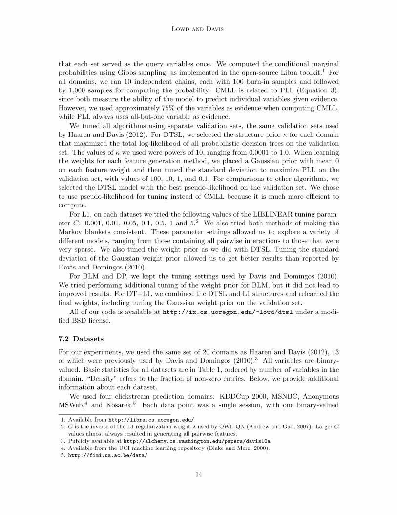
Figure 4: Number of features for each DTSL feature generation method on each dataset.Datasets are ordered by the number of features generated by the Defaultmethod.

balanced binary tree are leaves and the other half are interior nodes. Nonzero typicallyyields the shortest and the fewest rules, as expected.

7.4 Accuracy

We then compared DTSL, DT-BLM, and DT+L1 to three standard Markov network struc-ture learners: L1-regularized logistic regression (Ravikumar et al., 2010), BLM (Davis andDomingos, 2010), and DP (Della Pietra et al., 1997). For DTSL and DT-BLM, we used thefeature generation method that performed best on the validation set. In some cases, suchas KDDCup 2000, this was not the method that performed best on the test data.

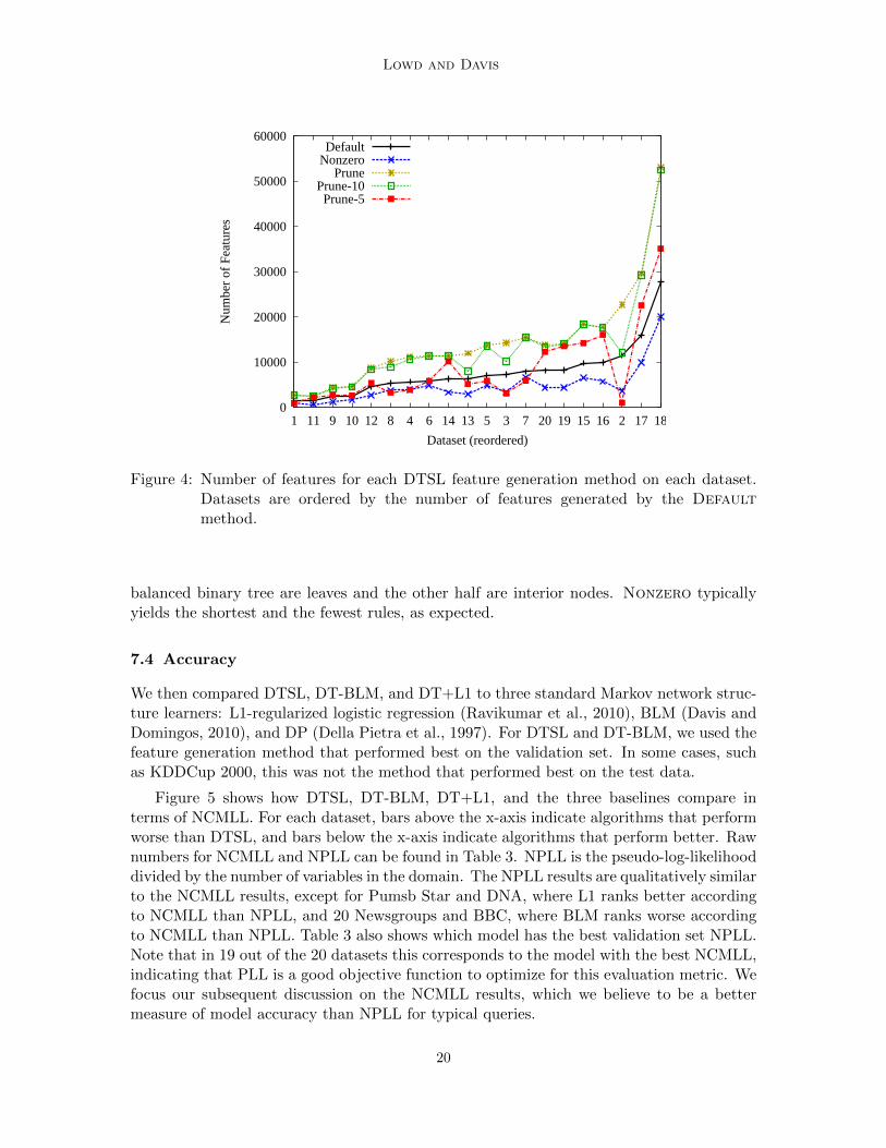
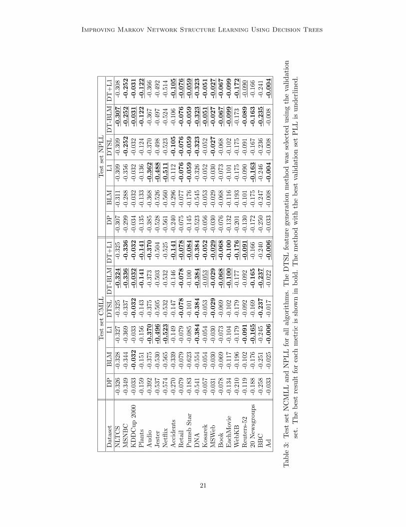
Figure 5 shows how DTSL, DT-BLM, DT+L1, and the three baselines compare interms of NCMLL. For each dataset, bars above the x-axis indicate algorithms that performworse than DTSL, and bars below the x-axis indicate algorithms that perform better. Rawnumbers for NCMLL and NPLL can be found in Table 3. NPLL is the pseudo-log-likelihooddivided by the number of variables in the domain. The NPLL results are qualitatively similarto the NCMLL results, except for Pumsb Star and DNA, where L1 ranks better accordingto NCMLL than NPLL, and 20 Newsgroups and BBC, where BLM ranks worse accordingto NCMLL than NPLL. Table 3 also shows which model has the best validation set NPLL.Note that in 19 out of the 20 datasets this corresponds to the model with the best NCMLL,indicating that PLL is a good objective function to optimize for this evaluation metric. Wefocus our subsequent discussion on the NCMLL results, which we believe to be a bettermeasure of model accuracy than NPLL for typical queries.

20


Tes

tse

tC

ML

LT

est

set

NP

LL

Dat

aset

DP

BL

ML

1D

TS

LD

T-B

LM

DT

+L

1D

PB

LM

L1

DT

SL

DT

-BL

MD

T+

L1

NLT

CS

-0.3

26-0

.328

-0.3

27

-0.3

25

-0.324

-0.3

25

-0.3

07

-0.3

11

-0.3

09

-0.3

09

-0.307

-0.3

08

MS

NB

C-0

.349

-0.3

44-0

.369

-0.3

37

-0.336

-0.336

-0.2

99

-0.2

88

-0.3

56

-0.252

-0.252

-0.252

KD

DC

up

2000

-0.0

33-0.032

-0.0

33

-0.032

-0.032

-0.032

-0.0

34

-0.0

32

-0.0

32

-0.0

32

-0.031

-0.031

Pla

nts

-0.1

59-0

.151

-0.1

56

-0.1

43

-0.141

-0.141

-0.1

35

-0.1

33

-0.1

36

-0.1

24

-0.122

-0.122

Au

dio

-0.3

92-0

.375

-0.370

-0.3

75

-0.3

73

-0.370

-0.3

85

-0.3

68

-0.362

-0.3

70

-0.3

67

-0.3

66

Jes

ter

-0.5

37-0

.530

-0.496

-0.5

05

-0.5

03

-0.5

04

-0.5

28

-0.5

26

-0.488

-0.4

98

-0.4

97

-0.4

92

Net

flix

-0.5

74-0

.565

-0.523

-0.5

32

-0.5

32

-0.5

25

-0.5

61

-0.5

60

-0.511

-0.5

23

-0.5

24

-0.5

14

Acc

iden

ts-0

.270

-0.3

39-0

.149

-0.1

47

-0.1

46

-0.141

-0.2

40

-0.2

96

-0.1

12

-0.105

-0.1

06

-0.105

Ret

ail

-0.0

79-0

.079

-0.0

79

-0.078

-0.078

-0.078

-0.0

75

-0.0

77

-0.076

-0.076

-0.076

-0.076

Pu

msb

Sta

r-0

.183

-0.6

23-0

.085

-0.1

01

-0.1

00

-0.084

-0.1

45

-0.1

76

-0.059

-0.059

-0.059

-0.059

DN

A-0

.541

-0.5

54-0.384

-0.384

-0.384

-0.384

-0.5

23

-0.5

45

-0.3

26

-0.323

-0.323

-0.323

Kos

arek

-0.0

57-0

.054

-0.0

54

-0.0

53

-0.0

53

-0.052

-0.0

56

-0.0

53

-0.0

52

-0.0

52

-0.051

-0.051

MS

Web

-0.0

31-0

.030

-0.0

30

-0.029

-0.029

-0.029

-0.0

30

-0.0

29

-0.0

30

-0.027

-0.027

-0.027

Book

-0.0

78-0

.069

-0.0

73

-0.0

69

-0.068

-0.068

-0.0

76

-0.0

68

-0.0

73

-0.0

68

-0.067

-0.067

Eac

hM

ovie

-0.1

34-0

.117

-0.1

04

-0.1

02

-0.100

-0.100

-0.1

32

-0.1

16

-0.1

01

-0.1

02

-0.099

-0.099

Web

KB

-0.2

10-0

.196

-0.1

79

-0.1

79

-0.1

77

-0.176

-0.2

01

-0.1

93

-0.1

75

-0.1

75

-0.1

73

-0.172

Reu

ters

-52

-0.1

19-0

.102

-0.091

-0.0

92

-0.0

92

-0.091

-0.1

30

-0.1

01

-0.0

90

-0.0

91

-0.089

-0.0

90

20N

ewsg

rou

ps

-0.1

88-0

.176

-0.165

-0.1

69

-0.165

-0.1

66

-0.1

72

-0.1

75

-0.163

-0.1

67

-0.163

-0.1

66

BB

C-0

.258

-0.2

51-0

.245

-0.237

-0.237

-0.2

40

-0.2

50

-0.2

47

-0.2

46

-0.2

36

-0.235

-0.2

41

Ad

-0.0

33-0

.025

-0.006

-0.0

17

-0.0

22

-0.006

-0.0

33

-0.0

08

-0.004

-0.0

08

-0.0

08

-0.004

Tab

le3:

Tes

tse

tN

CM

LL

and

NP

LL

for

all

algo

rith

ms.

Th

eD

TS

Lfe

atu

rege

ner

atio

nm

eth

od

was

sele

cted

usi

ng

the

vali

dat

ion

set.

Th

eb

est

resu

ltfo

rea

chm

etri

cis

show

nin

bol

d.

Th

em

eth

od

wit

hth

eb

est

vali

dat

ion

set

PL

Lis

un

der

lin

ed.

21

Lowd and Davis

−0.02

−0.01

0

0.01

0.02

0.03

0.04

0.05

0.06

1 2 3 4 5 6 7 8 9 10 11 12 13 14 15 16 17 18 19 20

Neg

ativ

e N

CM

LL r

elat

ive

to D

TS

L

Dataset

DPBLML1DT−BLMDT+L1

Figure 5: Normalized negative CMLL, relative to DTSL. Lower values indicate better per-formance. Positive values (above the x-axis) indicate methods that performedworse than DTSL, and negative values (below the x-axis) indicate methods thatperformed better than DTSL.

Overall, DP and BLM are fairly inaccurate, DTSL and L1 are roughly comparable,and DT-BLM is slightly better than DTSL. DT+L1 usually does at least as well as bothDTSL and L1, making it the most reliably accurate algorithm overall. DTSL is alwaysmore accurate than DP and BLM, except for three datasets where it is tied with BLM.DTSL is significantly more accurate than both DP and BLM (p < 0.001) according to aWilcoxon signed-ranks test in which the test set NCMLL of each dataset appears as onesample in the significance test. DT-BLM represents a modest improvement in accuracy overDTSL, performing slightly better than DTSL on 11 datasets and worse on only one. On theremaining eight datasets, the difference in NCMLL was less than 0.001. A Wilcoxon signed-ranks test indicates that DT-BLM is significantly more accurate than DTSL (p < 0.05).Since DT+L1 includes the features from both DTSL and L1, it usually does at least as wellas both methods, and sometimes better. DT+L1 is the most accurate method (includingties) on 15 out of 20 datasets, while DT-BLM is one of the most accurate methods on only11 datasets, DTSL on five, and L1 on seven. DT+L1 is more accurate than both L1 andDTSL (p < 0.05) according to a Wilcoxon signed-ranks test.

Comparisons between DTSL or DT-BLM and L1 are interesting because they demon-strate the relative strengths of using trees versus logistic regression for generating features.DTSL performs better than L1 on 11 datasets and worse on seven. Similarly, DT-BLMperforms better than L1 on 12 datasets and worse on six. These differences are not signif-icant according to a Wilcoxon signed-ranks test. The relative performance of DTSL and

22


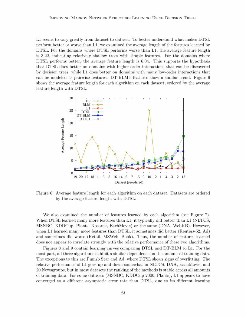
L1 seems to vary greatly from dataset to dataset. To better understand what makes DTSLperform better or worse than L1, we examined the average length of the features learned byDTSL. For the domains where DTSL performs worse than L1, the average feature lengthis 3.22, indicating relatively shallow trees with simple features. For the domains whereDTSL performs better, the average feature length is 6.04. This supports the hypothesisthat DTSL does better on domains with higher-order interactions that can be discoveredby decision trees, while L1 does better on domains with many low-order interactions thatcan be modeled as pairwise features. DT-BLM’s features show a similar trend. Figure 6shows the average feature length for each algorithm on each dataset, ordered by the averagefeature length with DTSL.

0

5

10

15

20

25

30

19 20 17 18 11 5 8 16 14 6 7 15 9 10 12 1 4 3 2 13

Ave

rage

Fea

ture

Len

gth

Dataset (reordered)

DPBLM

L1DTSL

DT-BLMDT+L1

Figure 6: Average feature length for each algorithm on each dataset. Datasets are orderedby the average feature length with DTSL.

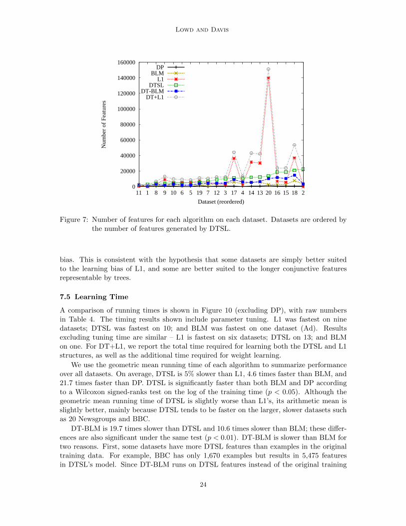
We also examined the number of features learned by each algorithm (see Figure 7).When DTSL learned many more features than L1, it typically did better than L1 (NLTCS,MSNBC, KDDCup, Plants, Kosarek, EachMovie) or the same (DNA, WebKB). However,when L1 learned many more features than DTSL, it sometimes did better (Reuters-52, Ad)and sometimes did worse (Retail, MSWeb, Book). Thus, the number of features learneddoes not appear to correlate strongly with the relative performance of these two algorithms.

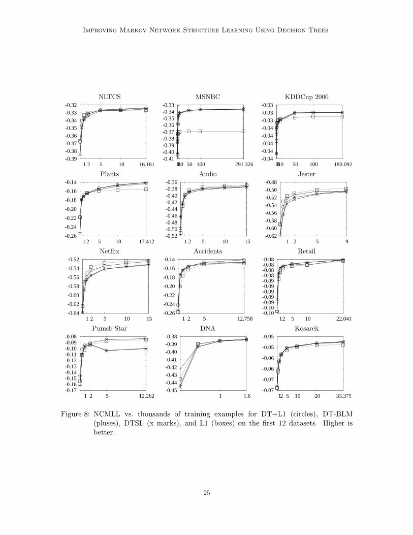
Figures 8 and 9 contain learning curves comparing DTSL and DT-BLM to L1. For themost part, all three algorithms exhibit a similar dependence on the amount of training data.The exceptions to this are Pumsb Star and Ad, where DTSL shows signs of overfitting. Therelative performance of L1 goes up and down somewhat in NLTCS, DNA, EachMovie, and20 Newsgroups, but in most datasets the ranking of the methods is stable across all amountsof training data. For some datasets (MSNBC, KDDCup 2000, Plants), L1 appears to haveconverged to a different asymptotic error rate than DTSL, due to its different learning

23

Lowd and Davis

0

20000

40000

60000

80000

100000

120000

140000

160000

11 1 8 9 10 6 5 19 7 12 3 17 4 14 13 20 16 15 18 2

Num

ber

of F

eatu

res

Dataset (reordered)

DPBLM

L1DTSL

DT-BLMDT+L1

Figure 7: Number of features for each algorithm on each dataset. Datasets are ordered bythe number of features generated by DTSL.

bias. This is consistent with the hypothesis that some datasets are simply better suitedto the learning bias of L1, and some are better suited to the longer conjunctive featuresrepresentable by trees.

7.5 Learning Time

A comparison of running times is shown in Figure 10 (excluding DP), with raw numbersin Table 4. The timing results shown include parameter tuning. L1 was fastest on ninedatasets; DTSL was fastest on 10; and BLM was fastest on one dataset (Ad). Resultsexcluding tuning time are similar – L1 is fastest on six datasets; DTSL on 13; and BLMon one. For DT+L1, we report the total time required for learning both the DTSL and L1structures, as well as the additional time required for weight learning.

We use the geometric mean running time of each algorithm to summarize performanceover all datasets. On average, DTSL is 5% slower than L1, 4.6 times faster than BLM, and21.7 times faster than DP. DTSL is significantly faster than both BLM and DP accordingto a Wilcoxon signed-ranks test on the log of the training time (p < 0.05). Although thegeometric mean running time of DTSL is slightly worse than L1’s, its arithmetic mean isslightly better, mainly because DTSL tends to be faster on the larger, slower datasets suchas 20 Newsgroups and BBC.

DT-BLM is 19.7 times slower than DTSL and 10.6 times slower than BLM; these differ-ences are also significant under the same test (p < 0.01). DT-BLM is slower than BLM fortwo reasons. First, some datasets have more DTSL features than examples in the originaltraining data. For example, BBC has only 1,670 examples but results in 5,475 featuresin DTSL’s model. Since DT-BLM runs on DTSL features instead of the original training

24


NLTCS MSNBC KDDCup 2000

-0.39-0.38-0.37-0.36-0.35-0.34-0.33-0.32

1 2 5 10 16.181

CM

LL

# Training Examples in 1000s

-0.41-0.40-0.39-0.38-0.37-0.36-0.35-0.34-0.33

0 1 2 5 10 50 100 291.326

CM

LL


-0.04-0.04-0.04-0.04-0.04-0.03-0.03-0.03

0 1 2 5 10 50 100 180.092

CM

LL

# Training Examples in 1000sPlants Audio Jester

-0.26

-0.24

-0.22

-0.20

-0.18

-0.16

-0.14

1 2 5 10 17.412

CM

LL


-0.52-0.50-0.48-0.46-0.44-0.42-0.40-0.38-0.36

1 2 5 10 15

CM

LL


-0.62-0.60-0.58-0.56-0.54-0.52-0.50-0.48

1 2 5 9

CM

LL

# Training Examples in 1000sNetflix Accidents Retail

-0.64

-0.62

-0.60

-0.58

-0.56

-0.54

-0.52

1 2 5 10 15

CM

LL


-0.26

-0.24

-0.22

-0.20

-0.18

-0.16

-0.14

1 2 5 12.758

CM

LL


-0.10-0.10-0.09-0.09-0.09-0.09-0.09-0.08-0.08-0.08-0.08

1 2 5 10 22.041

CM

LL

# Training Examples in 1000sPumsb Star DNA Kosarek

-0.17-0.16-0.15-0.14-0.13-0.12-0.11-0.10-0.09-0.08

1 2 5 12.262

CM

LL


-0.45-0.44-0.43-0.42-0.41-0.40-0.39-0.38

1 1.6

CM

LL


-0.07

-0.07

-0.06

-0.06

-0.05

-0.05

1 2 5 10 20 33.375

CM

LL


Figure 8: NCMLL vs. thousands of training examples for DT+L1 (circles), DT-BLM(pluses), DTSL (x marks), and L1 (boxes) on the first 12 datasets. Higher isbetter.

25

Lowd and Davis

MSWeb Book EachMovie

-0.04-0.04-0.04-0.04-0.04-0.03-0.03-0.03-0.03

1 2 5 10 20 29.441

CM

LL


-0.10

-0.09

-0.08

-0.08

-0.07

-0.07

-0.06

1 2 5 8.7

CM

LL


-0.15-0.14-0.14-0.13-0.13-0.12-0.12-0.11-0.11-0.10-0.10-0.09

1 2 4 4.524

CM

LL

# Training Examples in 1000sWebKB Reuters-52 20 Newsgroups

-0.22-0.21-0.21-0.20-0.20-0.19-0.19-0.18-0.18-0.17

1 2 2.803

CM

LL


-0.13-0.12-0.12-0.11-0.11-0.10-0.10-0.09-0.09

1 2 5 6.532

CM

LL


-0.20-0.20-0.19-0.18-0.18-0.17-0.17-0.16-0.16

1 2 5 11.293

CM

LL

# Training Examples in 1000sBBC Ad

-0.27-0.27-0.26-0.26-0.25-0.24-0.24-0.23

1 1.67

CM

LL


-0.12

-0.10

-0.08

-0.06

-0.04

-0.02

0.00

1 2 2.461

CM

LL


Figure 9: NCMLL vs. thousands of training examples for DT+L1 (circles), DT-BLM(pluses), DTSL (x marks), and L1 (boxes) on the last 8 datasets. Higher isbetter.

26


102

103

104

105

106

102 103 104 105 106

BL

M r

un ti

me

(s)

DTSL run time (s)

102

103

104

105

106

102 103 104 105 106

L1

run

time

(s)

DTSL run time (s)

103

104

105

106

107

102 103 104 105 106

DT

-BL

M r

un ti

me

(s)

DTSL run time (s)

102

103

104

105

106

102 103 104 105 106

DT

+L

1 ru

n tim

e (s

)

DTSL run time (s)

Figure 10: Running time on each dataset in seconds (y-axis) relative to DTSL’s runningtime (x-axis). Points below the line y=x represent datasets where DTSL wasslower than the other algorithm. All times include tuning.

data, more features means a longer running time. Second, DT-BLM is more sensitive to thewidth of the Gaussian prior than BLM is, so DT-BLM has one extra parameter to tune. Ifwe instead use the best Gaussian prior width from DTSL, the algorithm runs roughly fourtimes faster, but remains slower than BLM.

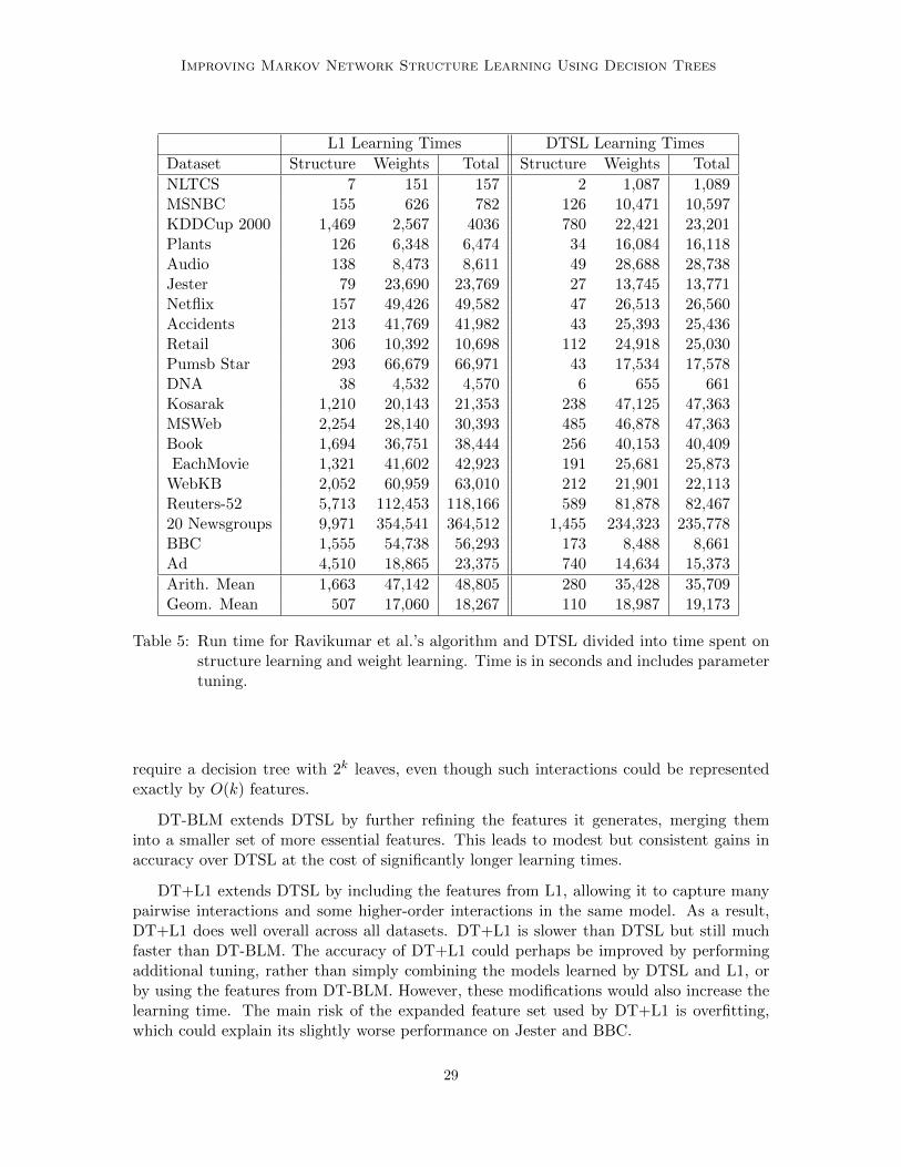
Table 5 shows a division of the total learning time, including tuning, divided into thetime spent learning the structure (i.e., the features) and the time spent on weight learning.With respect to the number of variables, DTSL has better scaling characteristics for featuregeneration than Ravikumar et al.’s L1 approach. The number of variables seems to have a

27

Lowd and Davis

Dataset DP BLM L1 DTSL DT-BLM DT+L1NLTCS 1,934 8,836 157 1,089 21,430 2,001MSNBC 438,611 116,315 782 10,597 2,533,367 19,606KDDCup 2000 335,398 51,744 4,036 23,201 1,012,635 30,463Plants 423,593 321,880 6,474 16,118 682,405 24,145Audio 653,111 402,441 8,611 28,738 155,970 45,829Jester 583,969 341,830 23,769 13,771 485,892 38,078Netflix 653,099 472,792 49,582 26,560 962,730 76,944Accidents 637,574 364,282 41,982 25,436 120,434 69,045Retail 279,507 384,011 10,698 25,030 405,059 36,090Pumsb Star 707,530 489,854 66,971 17,578 318,017 87,292DNA 197,406 1,666 4,570 661 6,635 7,365Kosarek 626,336 130,962 21,353 47,363 1,947,259 69,363MSWeb 426,199 83,727 30,393 47,363 2,635,238 78,579Book 641,338 72,398 38,444 40,409 1,405,667 82,966EachMovie 694,509 66,983 42,923 25,873 1,401,549 70,613WebKB 715,885 26,754 63,010 22,113 1,192,672 86,727Reuters-52 790,165 144,641 118,166 82,467 202,551 202,23720 Newsgroups 792,268 520,361 364,512 235,778 1,201,506 601,137BBC 864,000 8,944 56,293 8,661 12,352 66,197Ad 719,893 6,196 23,375 15,373 354,843 40,083Arith. Mean 559,116 200,831 48,805 35,709 852,911 86,738Geom. Mean 416,573 87,876 18,268 19,172 378,405 48,662

Table 4: Run time in seconds, including parameter tuning. The best run time is shown inbold.

greater effect on run time than the number of examples. Each additional variable requireslearning one extra model. Furthermore, each individual learning task is more complexbecause the target variable can depend on one additional input variable. The most strikingobservation is that the majority of time is spent learning the feature weights. For L1, onaverage, weight learning accounts for 93.8% of the total run time. For DTSL, this rises to99.1% of the total run time. The factor that most influences weight learning time is thenumber of features: models with more features lead to longer weight learning times. Thus,more efficient weight learning techniques would substantially improve the running time ofboth structure learning algorithms.

7.6 Discussion

Both DTSL and L1 are typically faster and more accurate than DP and BLM. DTSLexcels in domains that depend on higher-order interactions, while L1 performs better indomains that require many pairwise interactions. Therefore, neither algorithm dominatesor subsumes the other; rather, they discover complementary types of structure.

DTSL has two weaknesses. The first is a higher risk of overfitting, since it often generatesmany very specialized features. For the most part, this can be remedied with careful tuningon a validation set. The second is a limited ability to capture many independent interactions.For instance, to capture pairwise interactions between a variable and k other variables would

28


L1 Learning Times DTSL Learning Times

Dataset Structure Weights Total Structure Weights Total

NLTCS 7 151 157 2 1,087 1,089MSNBC 155 626 782 126 10,471 10,597KDDCup 2000 1,469 2,567 4036 780 22,421 23,201Plants 126 6,348 6,474 34 16,084 16,118Audio 138 8,473 8,611 49 28,688 28,738Jester 79 23,690 23,769 27 13,745 13,771Netflix 157 49,426 49,582 47 26,513 26,560Accidents 213 41,769 41,982 43 25,393 25,436Retail 306 10,392 10,698 112 24,918 25,030Pumsb Star 293 66,679 66,971 43 17,534 17,578DNA 38 4,532 4,570 6 655 661Kosarak 1,210 20,143 21,353 238 47,125 47,363MSWeb 2,254 28,140 30,393 485 46,878 47,363Book 1,694 36,751 38,444 256 40,153 40,409EachMovie 1,321 41,602 42,923 191 25,681 25,873

WebKB 2,052 60,959 63,010 212 21,901 22,113Reuters-52 5,713 112,453 118,166 589 81,878 82,46720 Newsgroups 9,971 354,541 364,512 1,455 234,323 235,778BBC 1,555 54,738 56,293 173 8,488 8,661Ad 4,510 18,865 23,375 740 14,634 15,373

Arith. Mean 1,663 47,142 48,805 280 35,428 35,709Geom. Mean 507 17,060 18,267 110 18,987 19,173

Table 5: Run time for Ravikumar et al.’s algorithm and DTSL divided into time spent onstructure learning and weight learning. Time is in seconds and includes parametertuning.

require a decision tree with 2k leaves, even though such interactions could be representedexactly by O(k) features.

DT-BLM extends DTSL by further refining the features it generates, merging theminto a smaller set of more essential features. This leads to modest but consistent gains inaccuracy over DTSL at the cost of significantly longer learning times.

DT+L1 extends DTSL by including the features from L1, allowing it to capture manypairwise interactions and some higher-order interactions in the same model. As a result,DT+L1 does well overall across all datasets. DT+L1 is slower than DTSL but still muchfaster than DT-BLM. The accuracy of DT+L1 could perhaps be improved by performingadditional tuning, rather than simply combining the models learned by DTSL and L1, orby using the features from DT-BLM. However, these modifications would also increase thelearning time. The main risk of the expanded feature set used by DT+L1 is overfitting,which could explain its slightly worse performance on Jester and BBC.

29

Lowd and Davis

8. Conclusions and Future Work

In this paper, we presented three new methods for using decision trees to learn the structureof Markov networks: DTSL, DT-BLM, and DT+L1.

DTSL is similar to the approach of Ravikumar et al. (2010), except that it uses decisiontrees in place of L1-regularized logistic regression. This allows it to learn longer featurescapturing interactions among more variables, which yields substantially better performancein several domains. DTSL is also similar to methods for learning dependency networks withtree conditional probability distributions (Heckerman et al., 2000). However, dependencynetworks may not represent consistent probability distributions and require that inferencebe done with Gibbs sampling, while the Markov networks learned by DTSL have neither ofthose limitations.

In terms of speed, we found that DTSL and L1-regularized logistic regression (Raviku-mar et al., 2010) had similar speed, while BLM (Davis and Domingos, 2010) and Della Pietraet al. (1997) were significantly slower. With a faster weight learning method, this compari-son would be even more favorable to DTSL and L1, since most of their time was spent onthe final weight learning step. In terms of accuracy, DTSL is comparable in accuracy toother approaches, placing ahead of all three baselines on nine out of 20 datasets.

The other two methods are extensions of DTSL that combine it with other structurelearning algorithms. DT-BLM builds on DTSL by running the BLM bottom-up structurelearning algorithm on the features generated by DTSL. This usually leads to slightly betteraccuracy, but is also much slower. DT+L1 extends DTSL by adding the features learned byL1-regularized logistic regression. This hybrid approach is very effective: DT+L1 is one ofthe most accurate methods on 15 out of 20 datasets and runs much faster than DT-BLM.

Future work includes exploring other methods of learning local structure, such as rulesets, boosted decision trees, and neural networks; determining sufficient conditions for theasymptotic consistency of local learning; further improving speed, perhaps by using frequentitemsets; and incorporating faster methods for weight learning, since structure learning isno longer the bottleneck.

Acknowledgments

The authors would like to thank the anonymous reviewers for many helpful suggestions.We also thank Jan Van Haaren for his valuable feedback on the article. DL is partlysupported by ARO grant W911NF-08-1-0242 and NSF grant IIS-1118050. The views andconclusions contained in this document are those of the authors and should not be inter-preted as necessarily representing the official policies, either expressed or implied, of AROor the United States Government. JD is partially supported by the research fund KU Leu-ven (CREA/11/015 and OT/11/051), and EU FP7 Marie Curie Career Integration Grant(#294068).

References

G. Andrew and J. Gao. Scalable training of l1-regularized log-linear models. In Proceedingsof the Twenty-Fourth International Conference on Machine Learning, pages 33–40. ACM

30


Press, 2007.

J. Besag. Statistical analysis of non-lattice data. The Statistician, 24:179–195, 1975.

C. Blake and C. J. Merz. UCI repository of machine learning databases. Machine-readabledata repository, Department of Information and Computer Science, University of Cali-fornia at Irvine, Irvine, CA, 2000. http://www.ics.uci.edu/∼mlearn/MLRepository.html.

F. Bromberg, D. Margaritis, and V. Honavar. Efficient Markov network structure discoveryusing independence tests. Journal of Artificial Intelligence Research, 35(2):449, 2009.

D. Chickering, D. Heckerman, and C. Meek. A Bayesian approach to learning Bayesiannetworks with local structure. In Proceedings of the Thirteenth Conference on Uncertaintyin Artificial Intelligence, pages 80–89, Providence, RI, 1997. Morgan Kaufmann.

J. Davis and P. Domingos. Bottom-up learning of Markov network structure. In Proceedingsof the Twenty-Seventh International Conference on Machine Learning, pages 271–278,Haifa, Israel, 2010. ACM Press.

S. Della Pietra, V. Della Pietra, and J. Lafferty. Inducing features of random fields. IEEETransactions on Pattern Analysis and Machine Intelligence, 19:380–392, 1997.

P. Domingos and G. Hulten. Mining high-speed data streams. In Proceedings of the SixthACM SIGKDD International Conference on Knowledge Discovery and Data Mining,pages 71–80, Boston, MA, 2000. ACM Press.

R.-E. Fan, K.-W. Chang, C.-J. Hsieh, X.-R. Wang, and C.-J. Lin. Liblinear: A library forlarge linear classification. Journal of Machine Learning Research, (9):1871–1874, 2008.

W. R. Gilks, S. Richardson, and D. J. Spiegelhalter, editors. Markov Chain Monte Carloin Practice. Chapman and Hall, London, UK, 1996.

K. Goldberg, T. Roeder, D. Gupta, and C. Perkins. Eigentaste: A constant time collabo-rative filtering algorithm. Information Retrieval, 4(2):133–151, 2001.

J. Van Haaren and J. Davis. Markov network structure learning: A randomized feature gen-eration approach. In Proceedings of the Twenty-Sixth National Conference on ArtificialIntelligence. AAAI Press, 2012.

D. Heckerman, D. M. Chickering, C. Meek, R. Rounthwaite, and C. Kadie. Dependencynetworks for inference, collaborative filtering, and data visualization. Journal of MachineLearning Research, 1:49–75, 2000.

G. Hulten and P. Domingos. Mining complex models from arbitrarily large databases inconstant time. In Proceedings of the Eighth ACM SIGKDD International Conference onKnowledge Discovery and Data Mining, pages 525–531, Edmonton, Canada, 2002. ACMPress.

R. Kohavi, C. Brodley, B. Frasca, L. Mason, and Z. Zheng. KDD-Cup 2000 organizers’report: Peeling the onion. SIGKDD Explorations, 2(2):86–98, 2000.

31

Lowd and Davis

A. Kulesza and F. Pereira. Structured learning with approximate inference. In Advancesin Neural Information Processing Systems 20, pages 785–792, 2007.

S.-I. Lee, V. Ganapathi, and D. Koller. Efficient structure learning of Markov networksusing L1-regularization. In Advances in Neural Information Processing Systems 19, pages817–824. MIT Press, 2007.

D. C. Liu and J. Nocedal. On the limited memory BFGS method for large scale optimization.Mathematical Programming, 45(3):503–528, 1989.

D. Lowd and J. Davis. Learning Markov network structure with decision trees. In Proceed-ings of the 10th IEEE International Conference on Data Mining (ICDM), pages 334–343,Sydney, Australia, 2010. IEEE Computer Society Press.

A. McCallum. Efficiently inducing features of conditional random fields. In Proceedingsof the Nineteenth Conference on Uncertainty in Artificial Intelligence, pages 403–410,Acapulco, Mexico, 2003. Morgan Kaufmann.

K. Murphy, Y. Weiss, and M. Jordan. Loopy belief propagation for approximate inference:An empirical study. In Proceedings of the Fifteenth Conference on Uncertainty in ArtificialIntelligence, pages 467–475. Morgan Kaufmann, Stockholm, Sweden, 1999.

P. Ravikumar, M. J. Wainwright, and J. Lafferty. High-dimensional ising model selectionusing L1-regularized logistic regression. Annals of Statistics, 38(3):1287–1319, 2010.

M. Schmidt and K. Murphy. Convex structure learning in log-linear models: Beyond pair-wise potentials. In Proceedings of the International Conference on Artificial Intelligenceand Statistics (AISTATS), 2010.

P. Spirtes, C. Glymour, and R. Scheines. Causation, Prediction, and Search. Springer, NewYork, NY, 1993.

I. Tsamardinos, L. Brown, and C. Aliferis. The max-min hill-climbing Bayesian networkstructure learning algorithm. Machine Learning, 65(1):31–78, 2006.

C. Ziegler, S. McNee, J. Konstan, and G. Lausen. Improving recommendation lists throughtopic diversification. In Proceedings of the 14th International World Wide Web Confer-ence, pages 22–32, 2005.

32

improving markov network structure learning using - lirias

Documents