improving robot navigation in structured outdoor...
TRANSCRIPT
Improving Robot Navigation in Structured Outdoor
Environments by Identifying Vegetation from Laser Data
Kai M. Wurm Rainer Kummerle Cyrill Stachniss Wolfram Burgard
Abstract—This paper addresses the problem of vegetationdetection from laser measurements. The ability to detect veg-etation is important for robots operating outdoors, since itenables a robot to navigate more efficiently and safely in suchenvironments. In this paper, we propose a novel approach fordetecting low, grass-like vegetation using laser remission values.In our algorithm, the laser remission is modeled as a functionof distance, incidence angle, and material. We classify surfaceterrain based on 3D scans of the surroundings of the robot.The model is learned in a self-supervised way using vibration-based terrain classification. In all real world experiments wecarried out, our approach yields a classification accuracy ofover 99%. We furthermore illustrate how the learned classifiercan improve the autonomous navigation capabilities of mobilerobots.
I. INTRODUCTION
Autonomous outdoor navigation is an active research field
in robotics. In most of the outdoor navigation scenarios in-
cluding autonomous cars, autonomous wheelchairs, surveil-
lance robots, or transportation vehicles, the classification of
the terrain plays an important role as most of the robots have
been designed for navigation on streets or paved paths rather
than on natural surfaces covered by grass or vegetation. The
navigation outside of paved paths might be uncomfortable
for passengers and might even introduce the risk of the robot
getting stuck. Furthermore, driving on grass will in general
increase wheel slippage and in this way increase potential
errors in the odometry. Accordingly, the robust detection of
vegetated areas is an important requirement for robots in any
of the above-mentioned situations.
In this paper, we propose a novel laser-based classification
approach that is especially suited for detecting low vegetation
typically found in structured outdoor environments such as
parks or campus sites. We classify surface terrain based on
3D scans of the surrounding of the robot in order to allow
the robot to take the classification result into account during
trajectory planning. It exploits an effect that is well known
from satellite image analysis: Chlorophyll which is found
in living plants strongly reflects near-IR light [13]. Often
used laser scanners such as the SICK LMS 291-S05 scanner
emit near-IR light and return the reflectivity of the object
they hit. Our approach models this remission value of the
laser scanner as a function of terrain class, incidence angle,
and measured distance. Classification is done using a support
All authors are with the University of Freiburg, Department of ComputerScience, D-79110 Freiburg, Germany
This work has partly been supported by the German Research Foundation(DFG) under contract number SFB/TR-8 (A3) and by the EC under contractnumber FP7-231888-EUROPA.
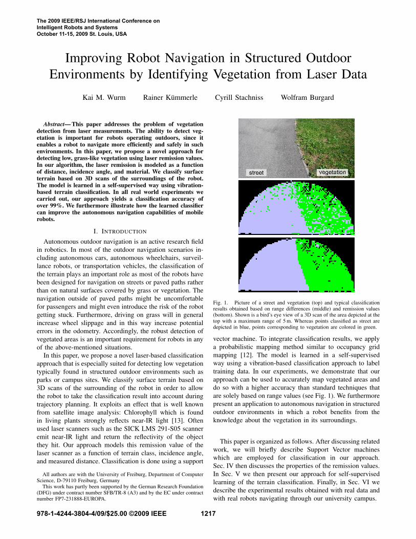
Fig. 1. Picture of a street and vegetation (top) and typical classificationresults obtained based on range differences (middle) and remission values(bottom). Shown is a bird’s eye view of a 3D scan of the area depicted at thetop with a maximum range of 5m. Whereas points classified as street aredepicted in blue, points corresponding to vegetation are colored in green.
vector machine. To integrate classification results, we apply
a probabilistic mapping method similar to occupancy grid
mapping [12]. The model is learned in a self-supervised
way using a vibration-based classification approach to label
training data. In our experiments, we demonstrate that our
approach can be used to accurately map vegetated areas and
do so with a higher accuracy than standard techniques that
are solely based on range values (see Fig. 1). We furthermore
present an application to autonomous navigation in structured
outdoor environments in which a robot benefits from the
knowledge about the vegetation in its surroundings.
This paper is organized as follows. After discussing related
work, we will briefly describe Support Vector machines
which are employed for classification in our approach.
Sec. IV then discusses the properties of the remission values.
In Sec. V we then present our approach for self-supervised
learning of the terrain classification. Finally, in Sec. VI we
describe the experimental results obtained with real data and
with real robots navigating through our university campus.
The 2009 IEEE/RSJ International Conference onIntelligent Robots and SystemsOctober 11-15, 2009 St. Louis, USA
978-1-4244-3804-4/09/$25.00 ©2009 IEEE 1217

II. RELATED WORK
There exist several approaches for detecting vegetation
using laser measurements. Wolf et al. [23] use hidden
Markov models to classify scans from a tilted laser scanner
into navigable (e.g., street) and non-navigable (e.g., grass)
regions. The main feature for classification is the variance
in height measurements relative to the robot height. Other
approaches analyze the distribution of 3D endpoints in a
sequence of scans [8], [9], [10]. However, flat vegetation
such as a freshly mowed lawn can not be reliably detected
using this feature alone.
A combination of camera and laser measurements has
been used to detect vegetation in several approaches [2],
[6], [11], [22]. In a combined system, Wellington et al. [22]
use the remission value of a laser scanner in addition
to density features and camera images as a classification
feature. However, they do not model the dependency between
remission, measured range, and incidence angle. Probably
due to this fact, they found the feature to be only ”moderately
informative”.
The approach that is closest to our approach has been
proposed by Bradley et al. [2]. Chlorophyll-rich vegetation
is detected using a combination of laser range measurements,
regular and near-infrared cameras. Vegetation is recognized
by comparing measurements from the different types of
cameras. 3D laser measurements of the environment are
projected into the camera images. A classifier is then trained
using the vegetation feature and features from the distribution
of 3D endpoints. According to the authors the approach
yields a classification accuracy of up to 95% but requires
sophisticated camera equipment.
In contrast to those combined systems, our approach uses
a laser scanner as its sole sensor. It is thus independent of
lighting conditions and can be used on a variety of existing
robot systems. Additionally, hand-labeling of training data is
not required in our approach.
Terrain types have also been classified using vibration
sensors on a robot [3], [7], [15], [21]. In these approaches,
the robot traverses the terrain and the induced vibration
is measured using accelerometers. The measurements are
usually analyzed in the Fourier domain. Sadhukhan et al. [15]
presented an approach based on neural networks. A similar
approach is presented by DuPont et al. [7]. Brooks and
Iagenemma [3] use a combination of principal component
analysis and linear discriminant analysis to classify terrain.
More recently, SVMs have been used by Weiss et al. [20],
[21].
Self-supervised learning has previously been used by
Dahlkamp et al. [5] in a vision-based road detection sys-
tem. Here, laser measurements are used to identify nearby
traversable surfaces. This information is then used to label
camera image patches in order to train a classifier that is able
to predict traversability in the far range. In our approach, we
adopt the idea of self-supervision to generate labeled training
data. We apply a vibration-based classifier to label laser
measurements recorded by the robot. This labeled dataset
is then used to train a laser-based vegetation classifier. Both
classifiers used in our approach have been implemented using
support vector machines which will be introduced in the
following.
III. SUPPORT VECTOR MACHINES
Support vector machines (SVMs) are a kernel-based learn-
ing method which is widely used for classification and
regression [16]. A SVM is essentially a hyperplane learning
algorithm. Two classes of data points are separated by a
hyperplane so that the margin between training points and
the plane is maximized:
maxw∈H,b∈R
min{||x − xi|| | x ∈ H, 〈w, x〉 + b = 0}, (1)
where H is some dot product space, xi are training points,
and w is a weighting vector. The following decision function
is used to determine the class label y:
f(x) = 〈w, x〉 + b (2)
y = sgn(f(x)) (3)
The hyperplane can be constructed efficiently by solving
a quadratic programming problem. To separate non-linear
classes, the so-called kernel trick is applied. The training
data is first mapped into a higher-dimensional feature space
using a kernel function. A separating hyperplane is then
constructed in this features space which yields a nonlinear
decision boundary in the input space. In practice, the Gaus-
sian Radial Basis Function (RBF) is often used as a kernel
function given by
k(x, x′) = e−(x−x
′)2
2l2 , (4)
with the so-called length-scale parameter l.
There exist derivatives of the basic SVM-formulation
which allow for training errors. Among those, C-SVM is a
popular method. An addition parameter commonly denoted
as C has to be optimized which adjusts the trade-off between
maximizing the margin and minimizing the training error.
Throughout this work, we use the SVM implementation
of LibSVM [4].
IV. USING REMISSION VALUES FOR
TERRAIN CLASSIFICATION
The goal of our terrain classification algorithm is to pre-
cisely classify the area containing vegetation. This classifica-
tion has to be made early enough for the robot’s planner to
take the classification into account. For this reason, we focus
on classifying three-dimensional scans of the environment
surrounding the robot.
We are interested in distinguishing flat vegetation such as
grass from drivable surfaces such as streets or paved paths.
For sake of brevity, we will call those classes of materials
”street” and ”vegetation” in the following.
Compared to an approach based purely on the scan point
distribution (see experiment in Sec. VI-A) a far better
classification accuracy can be achieved when the remission
value of laser measurements is used to classify endpoints.
1218

Fig. 2. Left: typical remission measurements of a SICK LMS 291-S05 forstreet (blue) and vegetation class (green). Right: mean remission values forboth classes.
Fig. 3. Classification of the scene depicted in Fig. 1 using the meanremission value (see Fig. 2, right) to distinguish both classes.
The SICK LMS laser scanner uses light at a wavelength of
905 nm which is within the near-infrared range. Chlorophyll
which is found in living plants strongly reflects near-IR
light [13]. The remission values returned by the scanner
depends on the material of the measured surface, on the
distance at which it is hit, and on the angle of incidence [1].
Unfortunately, this relation is non-linear as the example of
measurements in Fig. 2 shows. It is essential to take the
measured range as well as the angle of the measurement into
account. Averaging the remission value over all measured
ranges and angles will lead to wrong classification results
especially in the near range of up to three meters. This can
be seen in Fig. 3. Here, the scene from Fig. 1 was classified
using the mean remission value for both classes (see Fig. 2)
ignoring the range and incidence angle.
In our approach, we apply a C-SVM to classify laser
beams depending on the measured range, incidence angle,
and remission using a RBF-kernel. Other classification meth-
ods might certainly be used instead of a SVM as long as
they are able to classify data which is only separable in
a non-linear way. The input to the learning algorithm is a
labeled set of laser measurements. Each data point consists
of a range measurement, incidence angle, and a remission
value. By determining the separating hyperplane between
both data sets, we implicitly model the remission functions
for the street and vegetation class.
V. SELF-SUPERVISED LEARNING FOR
ROBUST TERRAIN CLASSIFICATION
To avoid tedious hand-labeling of dense three-dimensional
training data our algorithm uses a self-supervised training
method [5]. While the robot is moving it generates a 3D
model of the environment using the method described in
Sec. V-B. Incidence angles are estimated using the surface
normal in the 3D model as well as the angle of the laser
beam relative to the robot.
For each measured scan point the remission value, inci-
dence angle, and distance are stored. As the robot moves
through the environment it traverses previously scanned
surface patches. Those patches are labeled using the vibration
classifier described below and are then fed to the SVM as
training data. The training is done offline. To optimize the
length-scale parameter l of the kernel as well as the soft-
margin parameter C, we perform a systematic grid search
on the grid log2l ∈ {−15, ..., 3} and log
2C ∈ {−5, ..., 15}.
The optimal parameters are determined using 5-fold cross
validation.
Once the classifier has been trained, the model can be
used on any robot which is using the same sensor in a
similar configuration. More specifically, the laser should be
mounted so that the laser is measuring the surface at angles
and distances similar to those observed during the training
phase.
A. Terrain Classification based on the Vibration of the
Vehicle
We use a vibration-based classifier to label training data.
Different types of terrain induce vibrations of a different
characteristic to the robot. These vibrations can be measured
by an inertial measurement unit (IMU) and can be used
to classify the terrain the robot traverses. Note that such
classifiers do not allow the prediction of terrain classes in
areas which have not been traversed yet. In our system,
we only need to differentiate between vegetation and streets
(non-vegetation) to generate training data for the SVM.
In our experiments, we use a XSens MTi to measure the
acceleration along the z-axis. We apply the Fourier transform
to the raw acceleration data. In our algorithm, a 128-point
FFT is used to capture the frequency spectrum of up to 25Hz.
The frequency spectrum also depends on the speed of the
robot. To account for this dependency, it has been suggested
to train several classifiers at different speeds [20]. In our
system, however, we decided to treat the forward velocity
as a training feature instead. In addition to this, we also use
the rotational velocity as a feature to account for vibrations
which result from the skid-steering of our robot.
To classify the acceleration and velocity data, we again use
a C-SVM with a RBF-kernel. Our feature vector x consists
of the first 32 Fourier magnitudes |Fm|, the mean forward
velocity vt and the mean rotational velocity vr of the robot
over the sample period
|Fm| =√
(Re Fm)2 + (Im Fm)2,m∈{0,...,31} (5)
x = {|F0|, ..., |F31|, vt, rt}, (6)
where Fm denotes the m-th Fourier component. The classi-
fier was trained by recording short tracks of about 50m at
varying speeds both on a street and on vegetation. Parameter
optimization was done using grid search and 5-fold cross
validation.
1219

In our experiments, we achieved a high classification
accuracy and thus this data is well suited to label the training
data for the laser-based classification.
B. Mapping of Vegetation
We use multi-level surface maps [18] to model the envi-
ronment. This representation uses a 2D grid and stores in
each cell a set of patches representing individual surfaces
at different heights. In our approach, we additionally store
the probability of each surface patch to contain vegetation.
Let P (vi) denote this probability of patch i. In general,
surface patches will be observed multiple times. Therefore,
we need to probabilistically combine results from several
measurements. In this way, the uncertainty in classification
is explicitly taken into account.
Let zt be a laser measurement at time t. Analogous to
Moravec [12], we obtain an update rule for P (vi | z1:t).First we apply Bayes’ rule and obtain
P (vi | z1:t) =P (zt | v
i, z1:t−1)P (vi | z1:t−1)
P (zt | z1:t−1). (7)
We then compute the ratio
P (vi | z1:t)
P (¬vi | z1:t)=
P (zt | vi, z1:t−1)
P (zt | ¬vi, z1:t−1)
P (vi | z1:t−1)
P (¬vi | z1:t−1). (8)
Similarly, we obtain
P (vi | zt)
P (¬vi | zt)=
P (zt | vi)
P (zt | ¬vi)
P (vi)
P (¬vi),
which can be transformed to
P (zt | vi)
P (zt | ¬vi)=
P (vi | zt)
P (¬vi | zt)
P (¬vi)
P (vi). (9)
If we apply the Markov assumption that the current observa-
tion is independent of previous observations given we know
that a patch contains vegetation
P (zt | vi, z1:t−1) = P (zt | v
i) (10)
and utilize the fact that P (¬vi) = 1 − P (vi), we obtain
P (vi | z1:t)
1 − P (vi | z1:t)=
P (vi | zt)
1 − P (vi | zt)
P (vi | z1:t−1)
1 − P (vi | z1:t−1)
1 − P (vi)
P (vi). (11)
This equation can be transformed into the following update
formula:
P (vi | z1:t) =[
1 +1 − P (vi | zt)
P (vi | zt)
1 − P (vi | z1:t−1)
P (vi | z1:t−1)
P (vi)
1 − P (vi)
]−1
(12)
To perform the update step, we need an inverse sensor model
P (vi | z). In our system, this sensor model is based on the
remission value of the laser. The SVM-classifier is used to
model the measurement probabilities as described in the next
section. Here, the prior probability of P (vi) was set to 0.5.
Fig. 4. Robots used in our experiments.
C. Class Probabilities
The decision function of Support Vector Machines (see
Eq. 3) produces a class label y which is not a probability (y
is either 1 or -1).
Several methods have been proposed to map the output
of SVMs to posterior class probabilities [14], [19]. Among
those a popular approach is Platt’s method [14]. It uses a
parametric model to fit the posterior given by
P (y = 1 | f) = (1 + exp(Af + B))−1. (13)
The parameters A and B are determined using maximum
likelihood estimation from a training set (fi, yi), where fi
are the outputs of the function given in Eq. 2 and yi are the
corresponding class labels. For details of the optimization
step see [14]. In our approach, this method is used to obtain
the inverse sensor model P (vi | z).
VI. EXPERIMENTS
Our approach has been implemented and evaluated in
several experiments. The experiments are designed to demon-
strate that our approach is suitable to allow robots to reliably
detect vegetation and thus improves robust navigation in
structured outdoor environments.
We used two different robot systems (see Fig. 4). The self-
supervised learning approach is evaluated using an ActivMe-
dia Pioneer 2 AT, which is able to traverse low vegetation.
For mapping large environments and for an autonomous
driving experiment, we use an ActivMedia Powerbot plat-
form. This robot cannot safely traverse grass since its castor
wheels will block the robot due to its weight. Both robots
are equipped with SICK LMS S291-S05 laser scanners on
pan-tilt units. In addition to that, the Pioneer robot carries an
XSens MTi IMU to measure vibrations. Three-dimensional
scans are gathered by tilting the laser scanner from 50
degrees upwards to 30 degrees downwards. We use the raw
(unnormalized) remission values provided by the scanner.
We limit the classification to scans with a range smaller
than 5.0 meters. The approach itself is not limited in range.
However, at a laser resolution of one degree and a low height
of the sensor relative to the ground (approx. 0.5m), long
range data will be too sparse both to gather training data
and to reliably detect drivable surfaces and obstacles.
A. Vegetation detection using range differences
In a first experiment, we implemented a vegetation de-
tection algorithm based purely on the range differences of
1220

Fig. 5. Self-supervised learning. Left: the data set which is used to trainthe classifier. Right: test set recorded at a different location.
neighboring laser measurements similar to the one proposed
by Wolf et al. [23]. This method is only used for a com-
parison with our proposed classification approach. Three-
dimensional data is acquired by gathering a sweep of 2D
scans. For each 2D scan the 2D endpoints pi = 〈xi, yi〉 arecomputed from the range and angle measurements 〈ri, αi〉.A local feature di is then determined for every scan point
di = xi − xi−1. (14)
This feature captures the local roughness of the terrain. To
cope with flat but tilted surfaces we classify scans based
on the absolute difference in di between neighboring range
measurements as suggested in [11]. Furthermore, we also use
the measured range as a training feature to account for the
varying data density from near to far scans. A SVM is used
to train a classifier based on these features.
In our experiments, we achieve a classification accuracy
of about 75% using the described method. An example of
the classification results can be seen in Fig. 1. Similar results
have been reported by other researchers [2].
B. Self-supervised Learning
To train our remission-based classifier, we manually
steered the Pioneer AT robot through an outdoor environment
consisting of a street and an area covered with grass. We
acquired 3D scans approximately every 4m. While the robot
was driving the IMU measured the vibration induced to
the robot. To correct odometry errors of the robot, we em-
ployed a state-of-the-art SLAM approach [17] and 3D scan-
matching. We trained our classifier using the self-supervised
approach described in Sec. V. The training set is visualized in
Fig. 5a. The data recorded at the border region between street
and vegetation were ignored since the precise location of the
border cannot be determined using the vibration sensor. The
model for the laser-based classifier was trained using 19,989
vegetation and 11,248 street samples.
To further evaluate the precision of the classifier, we
recorded separate test data at a different location (see Fig. 5b
and Fig. 6). The test set contains 36,304 vegetation and
28,883 street measurements. Again, the labeling of the data
was carried out using the vibration-based classifier. The
previously trained classifier reached a precision of 99.9% on
the test data; the recall is 99.6%. The confusion matrix is
given in Table I. Note that such accurate classification results
are not due to overfitting. Fig. 2 illustrates that a non-linear
function (as learned by the SVM in our approach) can clearly
separate the classes.
TABLE I
CONFUSION MATRIX FOR EXP. VI-B (NUMBER OF DATA POINTS)
vegetation street
vegetation 36,300 138
street 4 28,745
Fig. 6. Aerial view of the computer science campus in Freiburg. Approxi-mated robot trajectories are shown for the training (top, yellow) and the testset (bottom, red). Courtesy of Google Maps, Copyright 2008, DigitalGlobe.
C. 3D Mapping
In this experiment, the Powerbot robot was steered across
the computer science campus at the University of Freiburg.
The scanning laser of the robot was tilted to a fixed angle
of 20 degrees downwards. In this way, a fairly large area
could be mapped in less than 15 minutes. The length of
the trajectory is 490m. The vegetation classifier was used
to map vegetation in the three-dimensional model of the
environment. To properly integrate multiple measurements,
we used the mapping approach described in Sec. V-B with
a cell size of 0.1m.
Due to a significantly different hardware setup than on the
Pioneer AT, we were not able to use the model generated in
Sec. VI-B. Instead, we recorded a training set of 12,153 grass
and 10,448 street samples by placing the robot in front of flat
areas containing only street and only vegetation. This method
is only applicable if such example data can be gathered
and thus should be considered inferior to the self-supervised
approach described in Sec. V.
Fig. 7. Mapping of a large outdoor environment. The laser was tilted at afixed angle of 20 degrees while the robot was moving. The figure shows a2D projection of the 3D map.
1221

Fig. 8. Autonomous navigation experiment. Although the shortest obstacle-free path from the start to the goal position led over grass, the robot couldreliably avoid the vegetated areas by using our vegetation classifier andtraveled over the paved streets to reach its goal.
Compared to the aerial image of the campus site in Fig. 6,
the mapping result shown in Fig. 7 is highly accurate. Even
small amounts of vegetation, for example between tiles on a
path, can be identified. To evaluate the accuracy of the map
created during this experiment, we manually marked wrongly
classified cells. Of a total of 271,638 cells (75,622 vegetation,
196,016 street), we found 547 false positives and 194 false
negatives. This corresponds to a precision of 99.23% and a
recall of 99.74%.
D. Autonomous Navigation
As mentioned above, the Powerbot cannot safely traverse
vegetated areas. In the experiment depicted in Fig. 8 (see
also our video attachment), the robot was told to navigate
to a goal position 80m in front while avoiding vegetation.
Since the robot did not have a map, it explored the envi-
ronment in the process of reducing its distance to the goal
location. Thereby, it used the vegetation classifier to detect
vegetation. The environment was represented as described in
Sec. V-B. Without knowledge about the specific terrain, the
shortest obstacle-free path would have led the robot across a
large area containing grass. By considering the classification
results in the path costs, however, the planner chose a safe
trajectory over the street.
VII. CONCLUSION
In this paper, we proposed a new approach to vegetation
detection using the remission values of a laser scanner.
By predicting vegetation in the surrounding of a robot,
our approach improves robot navigation in structured out-
door environments. The laser classifier is learned in a self-
supervised fashion by means of a support vector machine
using a vibration-based terrain classifier to gather training
data. The approach has been implemented and evaluated
in several real-world experiments. The experiments show
that our approach is able to accurately detect low, grass-
like vegetation with an accuracy of more than 99%. We also
demonstrated that the terrain classification can be used to
improve the navigation behavior of a robot.
Our current approach is limited to detecting flat vegetation
due to the self-supervised training method. In future work,
we will investigate whether the described approach can also
be applied to classify tall vegetation such as trees or bushes.
We will also look into using remission values provided by
the recently introduced Hokuyo UTM-30LX. With a weight
of 370 g this sensor could allow vegetation detection on an
even broader range of robots including humanoids and small
scale robots.
REFERENCES
[1] R. Baribeau, M. Rioux, and G. Godin. Color reflectance modelingusing a polychromatic laser range sensor. Pattern Analysis and
Machine Intelligence, IEEE Transactions on, 14(2):263–269, 1992.[2] D. Bradley, R. Unnikrishnan, and J. Bagnell. Vegetation detection for
driving in complex environments. In Proc. of the IEEE Int. Conf. on
Robotics & Automation (ICRA), 2007.[3] C.A. Brooks, K. Iagnemma, and S. Dubowsky. Vibration-based terrain
analysis for mobile robots. In Proc. of the IEEE Int. Conf. on Robotics
& Automation (ICRA), pages 3415–3420, 2005.[4] C-C. Chang and C-J. Lin. LIBSVM: a library for support vector
machines. http://www.csie.ntu.edu.tw/cjlin/libsvm, 2001.[5] H. Dahlkamp, A. Kaehler, D. Stavens, S. Thrun, and G. Bradski. Self-
supervised monocular road detection in desert terrain. In Proc. of
Robotics: Science and Systems (RSS), Philadelphia, USA, 2006.[6] B. Douillard, D. Fox, and F. Ramos. Laser and vision based outdoor
object mapping. In Proceedings of Robotics: Science and Systems IV,Zurich, Switzerland, 2008.
[7] E.M. DuPont, R.G. Roberts, C.A. Moore, M.F. Selekwa, and E.G.Collins. Online terrain classification for mobile robots. In Proc. of
the Int. Mechanical Engineering Congress and Exposition Conference
(IMECE), Orlando, USA, 2005.[8] M. Hebert and N. Vandapel. Terrain classification techniques from
ladar data for autonomous navigation. In Proc. of the Collaborative
Technology Alliances conference, College Park, MD., 2003.[9] J-F. Lalonde, N. Vandapel, D. Huber, and M. Hebert. Natural terrain
classification using three-dimensional ladar data for ground robotmobility. Journal of Field Robotics, 23(10):839 – 861, 2006.
[10] J. Macedo, R. Manduchi, and L. Matthies. Ladar-based discriminationof grass from obstacles for autonomous navigation. In ISER 2000:
Experimental Robotics VII, London, UK, 2001.[11] R. Manduchi, A. Castano, A. Talukder, and L.Matthies. Obstacle
detection and terrain classification for autonomous off-road navigation.Autonomous Robots, 18, pages 81–102, 2003.
[12] H.P. Moravec. Sensor fusion in certainty grids for mobile robots. AIMagazine, pages 61–74, 1988.
[13] R.B. Myneni, F.G. Hall, P.J. Sellers, and A.L. Marshak. The interpreta-tion of spectral vegetation indexes. IEEE Transactions on Geoscience
and Remote Sensing, 33(2):481–486, 1995.[14] J.C. Platt. Probabilistic outputs for support vector machines and
comparisons to regularized likelihood methods. In Advances in Large
Margin Classifiers, pages 61–74, 1999.[15] D. Sadhukhan, C. Moore, and E. Collins. Terrain estimation using
internal sensors. In Proc. of the IASTED Int. Conf. on Robotics and
Applications, Honolulu, Hawaii, USA, 2004.[16] B Scholkopf and A. Smola. Learning with Kernels. MIT Press, 2002.[17] C. Stachniss and G. Grisetti. GMapping project at OpenSLAM.org.
http://openslam.org, 2007.[18] R. Triebel, P. Pfaff, and W. Burgard. Multi-level surface maps for
outdoor terrain mapping and loop closing. In Proc. of the IEEE/RSJ
Int. Conf. on Intelligent Robots and Systems (IROS), 2006.[19] V.N. Vapnik. Statistical Learning Theory. Wiley-Interscience, 1998.[20] C. Weiss, N. Fechner, M. Stark, and A. Zell. Comparison of different
approaches to vibration-based terrain classification. In Proc. of the
European Conf. on Mobile Robots (ECMR), Freiburg, Germany, 2007.[21] C. Weiss, H. Frohlich, and A. Zell. Vibration-based terrain classi-
fication using support vector machines. In Proc. of the IEEE/RSJ
Int. Conf. on Intelligent Robots and Systems (IROS), 2006.[22] C. Wellington, A. Courville, and A. Stentz. A generative model of
terrain for autonomous navigation in vegetation. International Journalof Robotics Research, 25(12):1287 – 1304, 2006.
[23] D.F. Wolf, G. Sukhatme, D. Fox, and W. Burgard. Autonomous terrainmapping and classification using hidden markov models. In Proc. of
the IEEE Int. Conf. on Robotics & Automation (ICRA), 2005.
1222