Improving TDR/TDTMeasurements UsingNormalizationApplication Note 1304-5

2

TDR/TDT and NormalizationNormalization, an error-correction process, helps ensure that timedomain reflectometer (TDR) and time domain transmission (TDT)measurements are as accurate as possible. The Agilent 86100A wide-bandwidth oscilloscope includes normalization as a standard feature.With normalization software built into the oscilloscope, externalcontrollers and multiple step generators or risetime converters arenot needed. Normalization not only enhances measurement accuracy;it also simplifies the measurement process.

This application note discusses normalization and assumes the reader is familiar with basic TDR/TDT measurements. For back-ground on TDR/TDT measurements, refer to the on-line Help functionin the 86100A.

Time domain reflectometry (TDR) sends a very fast edge down atransmission line to a test device and then measures the reflectionsfrom that device. The measured reflections often make short work ofdesigning signal path interconnects and transmission lines in IC pack-ages, PC board traces, and coaxial connectors.

Time domain transmission (TDT) measurements are made by passingan edge through the test device. Parameters typically measured aregain and propagation delay. Transmission measurements also charac-terize crosstalk between traces.

Imperfect connectors, cabling, and even the response of the oscillo-scope itself can introduce errors into TDR/TDT measurements.Understanding the effects of these errors, and more importantly, howto remove them, will result in more accurate and useful measurements.

Normalization can be used in TDR/TDT measurements to remove theoscilloscope response, step aberrations, and cable losses and reflec-tions so that the only response measured is that of the device undertest (DUT). In addition, normalization can be used to predict how theDUT would respond to an ideal step of any arbitrary risetime.

Sources of Measurement ErrorThere are three primary sources of error in TDR/TDT measurements:the cables and connectors, the oscilloscope, and the step generator.

Cables and Connectors Cause Loss and ReflectionsCables and connectors between the step source, the DUT, and theoscilloscope can significantly affect measurement results. Impedancemismatches and imperfect connectors add reflections to the actualsignal being measured. These can distort the signal and make it diffi-cult to determine which reflections are from the DUT and which arefrom other sources.

In addition, cables are imperfect conductors that become more imper-fect as frequency increases. Cable losses, which increase at higherfrequencies, increase the risetime of edges and cause the edges todroop as they approach their final value.

3

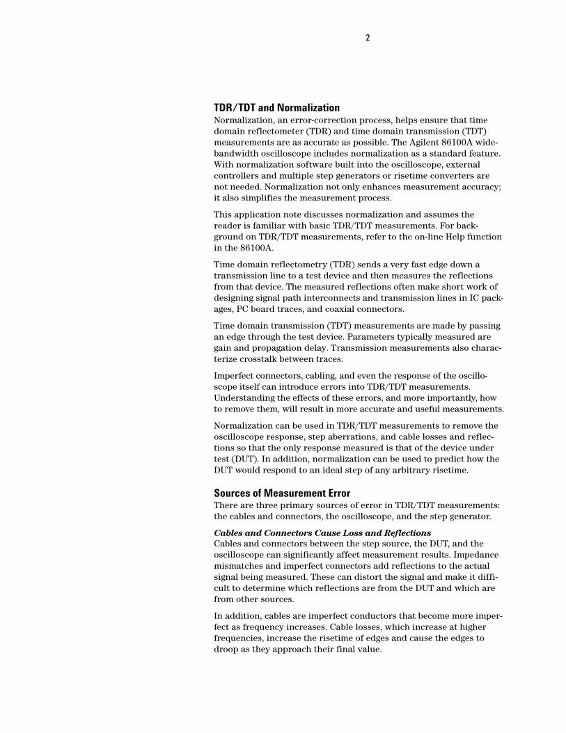
Figure 1 illustrates how cables and connec-tors affect TDR/TDT measurements. Theupper waveform is the reflection of a stepfrom a short circuit. Connections cause thereflections at the peak of the step and alongthe baseline. Cable loss yields the roundedtransition of the step to its baseline level.Normalization can correct the measureddata, resulting in the lower waveform.

The Oscilloscope as an Error SourceOscilloscopes introduce errors into measure-ments in several ways. The finite bandwidthof the oscilloscope translates to limited rise-time. Edges with risetimes less that theminimum risetime of the oscilloscope aremeasured slower than they actually are.When measuring how a device responds to avery fast edge, the oscilloscope’s limited rise-

time may distort or hide some of the device response.

The oscilloscope can also introduce small errors that are due to thetrigger coupling into the channels and channel crosstalk. These errorsappear as ringing and other non-flatness in the display of themeasurement channel baseline and are superimposed on themeasurement waveform. They are generally small and so are onlysignificant when measuring small signals.

The Step Generator as an Error SourceThe shape of the step stimulus is also important for accurateTDR/TDT measurements. The DUT responds not only to the step, but also to the aberrations on the step such as overshoot and non-flatness. If the overshoot is substantial, the DUT’s response can bemore difficult to interpret.

The risetime of the step is also extremely important. In most cases,the step generator used for TDR/TDT will have a fixed risetime. A hardware filter known as a risetime convertor can be used in somesystems to change the risetime.

To determine how the DUT will actually respond, you should test it atedge speeds similar to those it will actually encounter. Consider theexample of a BNC connector (Figure 2). Only about 3% of a 350 psrisetime edge (top waveform) is reflected by a BNC connector,whereas 6% of a 100 ps risetime edge (middle waveform) is reflected,and about 8% of a 50 ps risetime edge (bottom waveform) is reflected.

In the case of the measurement, the results obtained using a 50 psrisetime step stimulus do not apply for a connector that sees edgesthat are always slower than 350 ps. The connector might be accept-able for 350 ps edges but not for 50 ps edges. Measurements made atinappropriate risetimes can yield invalid conclusions.

Figure 1. The top waveform shows distortionscaused by cables and connectors. The bottomwaveform shows how normalization correctsfor these distortions.

4

Edge speed is also critical when usingTDR to locate the source of a disconti-nuity along a transmission line. Just asthe limited risetime of the oscilloscopecan limit the accuracy of this kind ofmeasurement, the risetime of the stepsource can also limit accuracy.

The risetime of the measurement systemis limited by the combined risetimes ofthe oscilloscope and the step generator. It can be approximated by Equation 1.

In a system with zero minimum risetime,the response of a discontinuity would notbe attenuated at all. A real system has alimited risetime, which acts as a lowpass

filter. If the step stimulus used is too slow,the true nature of the discontinuity may be disguised or may not evenbe visible. The cause may be more difficult to physically locate. Noticein Figure 2 that as the risetime of the step stimulus is decreased, thetrue nature of the reflection from the DUT becomes more apparent.

Removing Measurement ErrorsWaveform Subtraction Has LimitationsIn the past, waveform subtraction was used toreduce the effects of some of the errorsdiscussed above. It was convenient becausemany digitizing oscilloscopes provided this

feature without the aid of an external controller. A known good refer-ence device was measured, and the reference waveform stored inmemory. The reference waveform could then be subtracted from thewaveform measured from the DUT. The result showed how the DUTresponse differed from the reference response. This techniqueremoved error terms common to both the reference and the DUTwaveforms, such as trigger coupling, channel crosstalk, and reflec-tions from the cables and connectors.

Waveform subtraction has, however, several shortcomings. First, itrequires that a known good reference DUT exists and is available tomeasure. In some cases a good DUT may not be readily available ormay not exist at all. Second, the waveform which results from thesubtraction process is a description of how the DUT response differsfrom the reference response. Hence, there is no way to view the actualDUT response without the errors introduced by the test system.

Finally, the most significant shortcoming is that the measurementsare limited to the risetime of the test system. Determining the DUTresponse at multiple risetimes is cumbersome. Either multiple stepgenerators or multiple risetime convertors are necessary and a sepa-rate reference waveform is required for each risetime.

Figure 2. Variable edge speed helps determinethe amount of reflection in actual applications.The top waveform (tested to 350 ps) showsless reflection than the middle waveform(tested at 100 ps) or the bottom waveform(tested to 50 ps).

System risetime =

√(Step risetime)2 + (Scope risetime)2 + (Test setup-up risetime)2

Equation 1

5

Normalization Improves on Error CorrectionA digital error-correction method known as normalization can signifi-cantly reduce or remove all the above types of errors from TDR/TDTmeasurements. Taking full advantage of its powerful internal micropro-cessor, the Agilent 86100A Infiniium DCA (digital communicationsanalyzer) is a wide-bandwidth oscilloscope that includes normalizationas a standard feature.

Normalization can predict how the DUT will respond to an ideal step ofthe user-specified risetime. Only one step generator and one calibra-tion process are required. No risetime convertors are necessary, andthe calibration standards are not related to the DUT.

Unlike a risetime convertor, normalization can also increase the band-width (i.e., decrease the risetime) of the system by some amountdepending on the noise floor. This means that when more bandwidth iscritical, such as when trying to locate a discontinuity along a transmis-sion line, the waveform data acquired by the oscilloscope can be"squeezed" for every bit of useful information it contains.

Examples of What Normalization Can DoThe following two examples illustrate whatnormalization can accomplish:

Example 1: Correcting for the TDRmeasurement errors introduced byconnecting hardware.Consider trying to model a device at theend of some imperfect test fixture as inFigure 3.

This example uses two identical printedcircuit boards (PCBs) to model thismeasurement. The PCBs have a 50 Ωtrace on them with two discontinuities.The first PCB represents the test fixture,and the second PCB represents the DUT.The goal is to accurately measure thereflections caused by the DUT (secondPCB). Figure 4 is the unnormalizedresponse of the system.

The TDR response shows the reflectionsof the second PCB to be different fromthe first PCB. TDR accurately measuresthe first discontinuity. But TDR measureseach succeeding discontinuity with lessaccuracy, as the transmitted stepdegrades and multiple reflections occur.Thus the two identical boards showdifferent responses.

Figure 3. Test system with the device at theend of an imperfect test fixture.

TDRTest

Fixture

Device UnderTest

Figure 4. In an unnormalized measurement,the reflections from the DUT are masked by the

imperfect test fixture.

6

By defining a reference plane to be at the end ofthe test fixture (first PCB) and then normalizing,the errors can be corrected.

Calibration first defines a reference plane andgenerates a digital filter. The normalizingmeasurement then corrects for the errors intro-duced by the test fixture. Notice how the normal-ized response of the second PCB (DUT) (Figure6) now matches the response measured earlier ofthe nearly identical first PCB. (Figure 4)

To further verify the accuracy of the normaliza-tion, the response of the second PCB ismeasured without the first PCB. (Figure 7)

Example 2: Resolving two discontinuities sepa-rated by 2 mm.Normalization can improve the TDR’s ability toresolve adjacent discontinuities. Figure 8 showsthe TDR measurement results of two capacitivediscontinuities 2 mm apart in an air dielectric.Note that at a system risetime slower than 90 ps,the two discontinuities appear to be one. Bynormalizing the response to a system risetime of45 ps, both discontinuities can be seen.

Figure 5. A normalized calibration uses first a short, then a 50 Ωtermination to define a reference plane and generate a digital filter.

Figure 6. The normalized measurement corrects for the errorsintroduced by the test fixture.

Figure 7. The unnormalized response of the DUT, measured withoutthe test fixture.

Figure 8. Normalization improves the ability to distinguish twodiscontinuities by decreasing the system risetime.

7

Calibration Characterizes the Test SystemCalibration makes the normalization process possible. Calibrationmeasurements, which characterize the test system, are made with allcables and connections in place but without the DUT.

TDR/TDT can be accomplished with an oscilloscope and step gener-ator or with a frequency-domain network analyzer and sweptsinewave source. Normalization may be applied in either case.However, the calibration process for the network analyzer/sweptsource solution requires three measurements whereas only two arerequired for the oscilloscope/step generator solution.

Removing Systematic ErrorsThe first part of TDR/TDT calibration removes systematic errors dueto trigger coupling, channel crosstalk, and reflections from cables andconnectors.

For TDR calibration, the DUT is replaced by a short circuit. Thefrequency response of the test system is derived from the measuredshort. Note that a short circuit should be used rather than an opencircuit. When a step hits an open circuit at the end of a real-worldtransmission line, some of the energy is lost due to radiation ratherthan being reflected. Therefore, it is important that a good qualityshort be used, because the calibration process assumes a perfect shortcircuit termination. Any non-ideal components in the measured shortare attributed to the test system. If any of the non-ideal componentsare, in reality, due to the short itself, the filter will attempt to correctfor error terms that do not exist in the test system. By attempting tocorrect for errors that do not exist, the filter can actually add errorterms into the normalized measurement results.

Generating the Digital FilterThe second part of the calibration generates the digital filter. Unlikethe errors removed by subtracting the first calibration signal, theerrors removed by the filter are proportional to the amplitude of theDUT response.

For TDR, this is done by replacing the DUT with a termination havingan impedance equal to the characteristic impedance of the transmis-sion line, typically 50Ω. If the termination is properly matched, all ofthe energy that reaches it will be absorbed. The only reflectionsmeasured result from discontinuities along the transmission line.

In both cases, the measured waveforms are stored and subtracteddirectly from the measured DUT response before the response isfiltered. Ideally, these calibration waveforms are flat lines. Any non-flatness or ringing is superimposed on the measured DUT responseand represents a potential measurement error source. These errorsare not related to the magnitude of the response of the DUT.Therefore, it is valid to subtract them directly.

8

For TDT calibration, the transmission through-path is connectedwithout the DUT. The frequency response of the test system is thenmeasured with the aid of the step stimulus. With this information, adigital filter can be computed that will compensate for errors due toanomalies in the frequency response of the test system.

Correcting for Secondary ReflectionsSecondary reflections caused by the impedance mismatch betweenthe test port and the transmission media can also be corrected. Withthe oscilloscope/step generator TDR/TDT solution, airlines can sepa-rate the primary reflection from the secondary reflection. Timewindowing can then be used to remove the secondary reflections.With the network analyzer/swept source solution, a third calibrationis used.

The impedance mismatch between test port and transmission mediareflects a portion of the primary reflection back towards the DUT. Asecondary reflection from the DUT may then be measured. Secondaryreflections are usually very small.

Figure 9 shows the relative size of primary and secondary reflections.The lower waveform is a copy of the upper waveform with the voltagescale greatly expanded about the baseline to show more clearly theshape of the secondary reflection. The DUT is a short circuitconnected to the Agilent 86100A through a BNC connector. Asecondary reflection from the DUT is visible at the right end of the

baseline. Notice that the secondary reflec-tion is indeed quite small. It has a peakvoltage value of about 1.5 mV at 40 psrisetime, which is about 0.75% of the 200mV incident step.

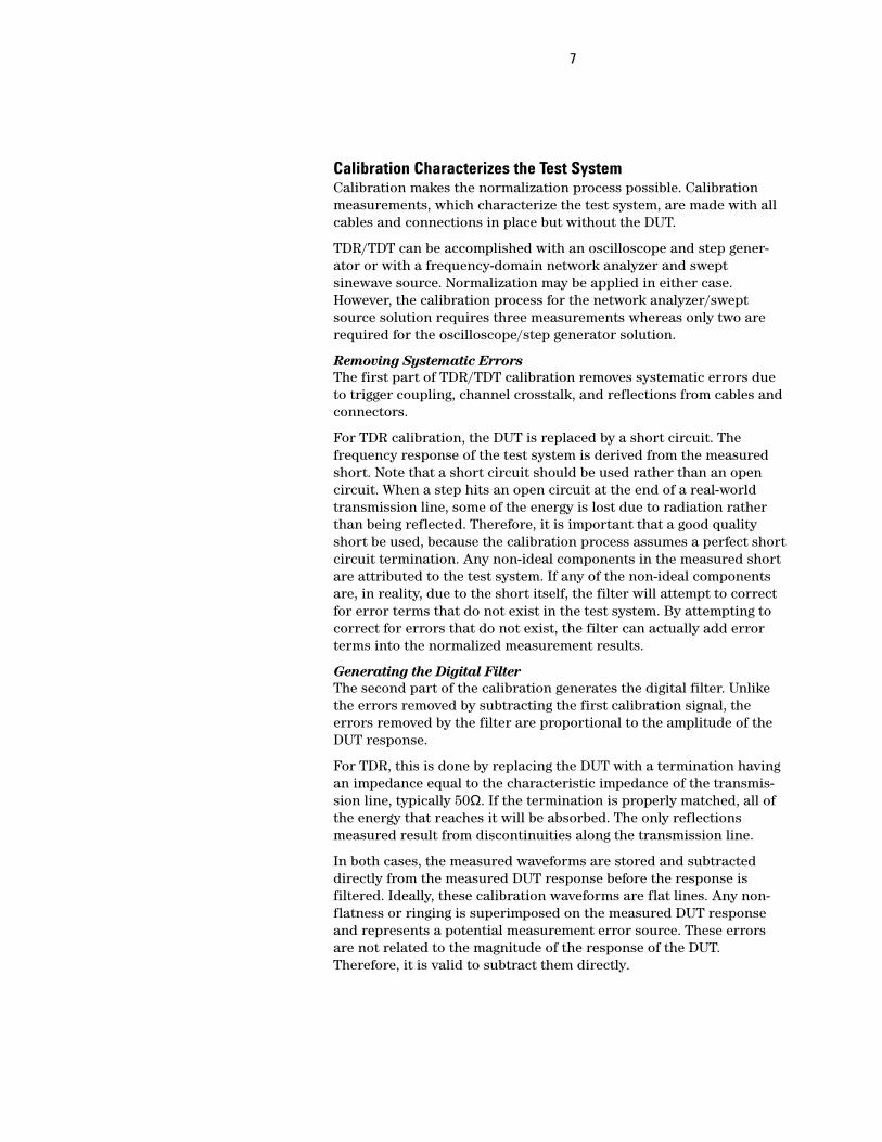
In TDR/TDT measurements made with anoscilloscope/step generator, a section ofairline may be placed between the testport and the DUT to provide time separa-tion between the primary reflection andsecondary reflections. Figure 10 illus-trates the use of this technique. Asecondary reflection is visible very closeto the primary reflection in the top wave-form. It is difficult to tell them apart. Ashort section of airline was placedbetween the DUT and the test port,resulting in the lower waveform. Note that

the primary and secondary reflections areclearly separated. When the primary and secondary reflections areclose together, the shapes of both may be distorted. If they areadequately separated in time, as is the case in the lower waveform,they no longer have a significant effect on each other.

After an adequate separation has been achieved, a time window canbe selected which does not include the undesirable secondary reflec-

Figure 9. The lower waveform is a copy of theupper waveform with the voltage scale greatlyexpanded about the baseline to show moreclearly the shape of the secondary reflection.

9

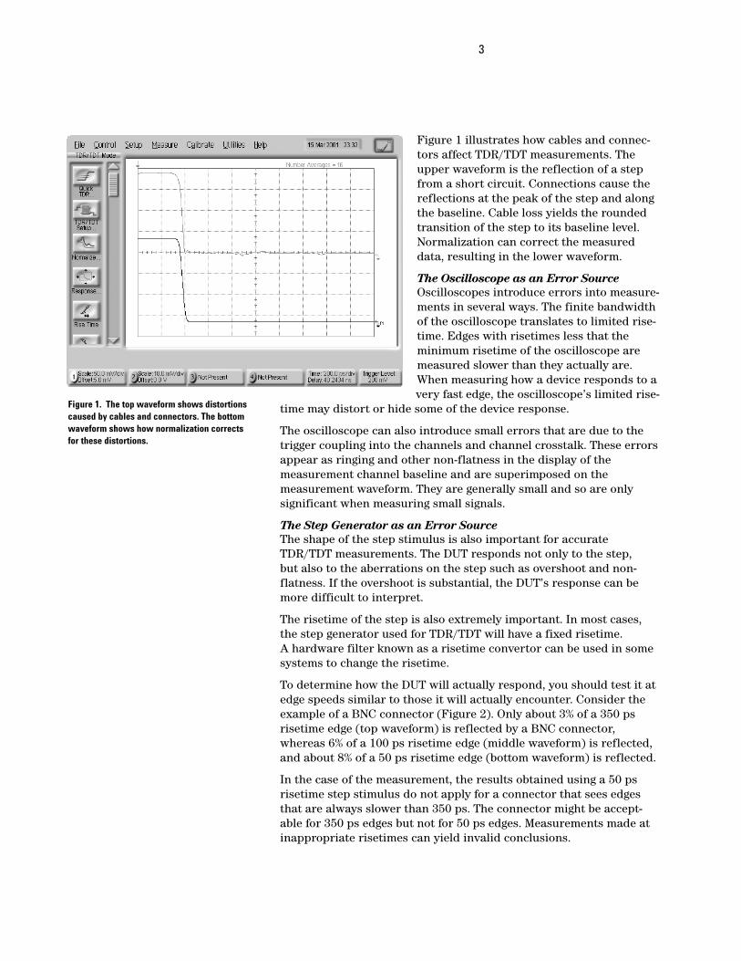
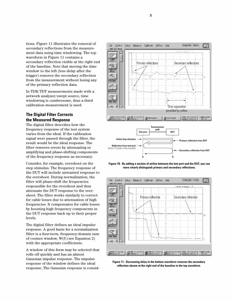
tions. Figure 11 illustrates the removal ofsecondary reflections from the measure-ment data using time windowing. The topwaveform in Figure 11 contains asecondary reflection visible at the right endof the baseline. Note that moving the timewindow to the left (less delay after thetrigger) removes the secondary reflectionfrom the measurement without losing anyof the primary reflection data.

In TDR/TDT measurements made with anetwork analyzer/swept source, timewindowing is cumbersome, thus a thirdcalibration measurement is used.

The Digital Filter Corrects the Measured ResponseThe digital filter describes how thefrequency response of the test systemvaries from the ideal. If the calibrationsignal were passed through the filter, theresult would be the ideal response. Thefilter removes errors by attenuating oramplifying and phase-shifting componentsof the frequency response as necessary.

Consider, for example, overshoot on thestep stimulus. The frequency response ofthe DUT will include unwanted response tothe overshoot. During normalization, thefilter will phase-shift the frequenciesresponsible for the overshoot and thusattenuate the DUT response to the over-shoot. The filter works similarly to correctfor cable losses due to attenuation of highfrequencies. It compensates for cable lossesby boosting high frequency components inthe DUT response back up to their properlevels.

The digital filter defines an ideal impulseresponse. A good basis for a normalizationfilter is a four-term, frequency-domain sumof cosines window, W(f) (see Equation 2)with the appropriate coefficients.

A window of this form may be selected thatrolls off quickly and has an almostGaussian impulse response. The impulseresponse of the window defines the idealresponse, The Gaussian response is consid-

Test port

Transmissionpath

Initial step stimulus

DUT

Reflection from test port(about 1% peak in this example)

Primary reflection from DUT

Secondary reflection from DUT

Figure 10. By adding a section of airline between the test port and the DUT, you canmore clearly distinguish primary and secondary reflections.

Figure 11. Decreasing delay in the bottom waveform removes the secondaryreflection shown at the right end of the baseline in the top waveform.

ered ideal because it has a minimum settling time after a transitionfrom one voltage level to another. Minimizing the settling time mini-mizes the interference between closely-spaced discontinuities, thusmaking them easier to see and analyze. The filter’s bandwidth, andtherefore risetime, is determined by the choice of L, the width of thesum of the cosines window. The actual normalization filter, F(f), iscomputed by dividing the sum of cosines window by the frequencyresponse of the test system, S(f) (see Equation 3). Frequencyresponse is the Fourier transform of the impulse response.

By varying the bandwidth of the filter, normalization can predict howthe DUT would respond to ideal steps of various risetimes. The band-width of the test system is the frequency at which the frequencyresponse is attenuated by 3 dB. The response beyond the cutofffrequency is not zero; it is only attenuated (Figure 12). By carefullychanging the –3 dB point in the frequency response, the bandwidthcan be increased or decreased.

In the Agilent 86100A, the user-specified risetime determines thebandwidth of the filter. Decreasing the bandwidth is accomplished byattenuating the frequencies that are beyond the bandwidth of interest(Figure 13). Increasing the bandwidth requires more consideration.

To increase the bandwidth, the response beyond the initial –3 dBfrequency needs to be amplified. While this is a valid step, it is impor-tant to realize that the system noise at these frequencies and atnearby higher frequencies is also amplified (see Figure 14).

The limit to which the risetime of real systems may be extended, isdetermined by the noise floor. In real systems,there is a point beyond which the amplitudeof the frequency response data is below thenoise floor. Any further increase in bandwidthonly adds noise.

Because waveform averaging reduces theinitial level of the noise floor, WAVEFORMAVERAGING SHOULD BE USED WHENNORMALIZING.

An equation can be used to describe thefiltering process. The test system frequencyresponse, S(f), can be thought of as the idealfrequency response defined by the sum ofcosines window, W(f), multiplied by an errorfrequency response, E(f) (see Equation 4).Further, the measured response of the DUT,M(f), can be thought of as the DUT frequencyresponse, D(f), multiplied by the test systemfrequency response, S(f). Filtering is accom-plished by multiplying the measuredfrequency response of the DUT by the filter, F(f). N(f) is the

10

Log (amplitude)

Noise floor

Log (frequency) Cutoff frequency

0 dB–3 dB

Log (amplitude)

Noise floor

Log (frequency)

New cutoff frequency Initial cutoff frequency0 dB

–3 dBFrequency components attenuated to reduce bandwidth

Basic system response

Normalized system response

Figure 12. Basic system frequency response.

Figure 13. Normalized system frequency response (system bandwidth reduced).

3W(f) = ∑ ak COS (2 πf k/L): for -L < f < L

2 2k = 0

= 0 elsewhere

where: a0 + a1 + a2 + a3 = 1

L = the full width of the window in hertz

f = frequency in hertz

F (f) = W(f)S(f)

Equation 2

Equation 3

11

normalized (filtered) frequencyresponse of the DUT. Equation 5describes the filtering processusing the above definitions.

The normalized response is theDUT frequency response multi-plied by the frequency response ofan ideal impulse. Note that theerror response has been removed,and that N(f) is an impulseresponse.

When N(f) is converted to thetime domain,1 the result is ni (t), a normalized impulse response.

Because a step stimulus is used, a normalized step response, ns(t), is desired. An ideal step canbe defined in the time domain byconvolving w(t), the ideal impulseresponse, with u(t), the unit stepfunction. Given this modification,Equation 6 further describes theeffect of the filtering process.

The normalized response, ns (t),is the impulse response of theDUT convolved with the ideal stepdefined by the convolution of w(t)with u(t). The result of normaliza-tion is, therefore, the response ofthe DUT to an ideal step of rise-time determined by w(t). Byvarying the width, L, of W(f),normalization can predict theresponse of the DUT at multiplerisetimes based on a single-stepresponse measurement.

Putting It All Together The actual normalization of aDUT response is accomplished intwo steps. A stored waveform,derived in the calibration andwhich represents the systematicerrors, is subtracted from themeasured DUT waveform. Thisresult is then convolved with thedigital filter to yield the response

Log (amplitude)

Noise floor

Log (frequency)

Initial cutoff frequency

Increased noise flooras a result of increasing

bandwidth

New cutoff frequency0 dB

–3 dB Frequency components amplified to increase bandwidth

Normalized system response

Basic system response

Figure 14. Normalized system frequency response (system bandwidth increased).

S(f) = W(f) E(f)

Equation 4

M(f) = D(f) S(f)N(f) = M(f) F(f)N(f) = D(f) S(f) F(f)

W(f)N(f) = D(f) W(f) E(f)

W(f) E(f)N(f) = D(f) W(f)

Equation 5

ni(t) = d(t) * w(t)ns(t) = ni(t) * u(t)ns(t) = d(t) * [w(t) * u(t)]

Equation 6

1 The Bracewell transform is under license from Stanford University.

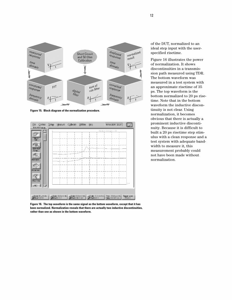
12

of the DUT, normalized to anideal step input with the user-specified risetime.

Figure 16 illustrates the powerof normalization. It showsdiscontinuities in a transmis-sion path measured using TDR.The bottom waveform wasmeasured in a test system withan approximate risetime of 35ps. The top waveform is thebottom normalized to 20 ps rise-time. Note that in the bottomwaveform the inductive discon-tinuity is not clear. Usingnormalization, it becomesobvious that there is actually aprominent inductive disconti-nuity. Because it is difficult tobuilt a 20 ps risetime step stim-ulus with a clean response and atest system with adequate band-width to measure it, thismeasurement probably couldnot have been made withoutnormalization.

Figure 15. Block diagram of the normalization procedure.

Figure 16. The top waveform is the same signal as the bottom waveform, except that it hasbeen normalized. Normalization reveals that there are actually two inductive discontinuities,rather than one as shown in the bottom waveform.

Agilent Technologies’Test and Measurement Support, Services, and AssistanceAgilent Technologies aims to maximize the value you receive, while minimizing your risk andproblems. We strive to ensure that you get the test and measurement capabilities you paid for andobtain the support you need. Our extensive support resources and services can help you choosethe right Agilent products for your applications and apply them successfully. Every instrumentand system we sell has a global warranty. Support is available for at least five years beyond theproduction life of the product. Two concepts underlie Agilent’s overall support policy: “OurPromise” and “Your Advantage.”

Our PromiseOur Promise means your Agilent test and measurement equipment will meet its advertisedperformance and functionality. When you are choosing new equipment, we will help you withproduct information, including realistic performance specifications and practical recommend-ations from experienced test engineers. When you use Agilent equipment, we can verify that itworks properly, help with product operation, and provide basic measurement assistance for theuse of specified capabilities, at no extra cost upon request. Many self-help tools are available.

Your AdvantageYour Advantage means that Agilent offers a wide range of additional expert test and measurementservices, which you can purchase according to your unique technical and business needs. Solveproblems efficiently and gain a competitive edge by contracting with us for calibration, extra-costupgrades, out-of-warranty repairs, and on-site education and training, as well as design, systemintegration, project management, and other professional engineering services. Experienced Agilentengineers and technicians worldwide can help you maximize your productivity, optimize thereturn on investment of your Agilent instruments and systems, and obtain dependablemeasurement accuracy for the life of those products.

By internet, phone, or fax, get assistance with all your test & measurement needs.

Online assistance:www.agilent.com/comms/tdrwww.agilent.com/find/si

Phone or FaxUnited States:(tel) 1 800 452 4844

Canada:(tel) 1 877 894 4414(fax) (905) 282 6495

Europe:(tel) (31 20) 547 2323(fax) (31 20) 547 2390

Japan:(tel) (81) 426 56 7832(fax) (81) 426 56 7840

Latin America:(tel) (305) 269 7500(fax) (305) 269 7599

Australia:(tel) 1 800 629 485 (fax) (61 3) 9210 5947

New Zealand:(tel) 0 800 738 378 (fax) 64 4 495 8950

Asia Pacific:(tel) (852) 3197 7777(fax) (852) 2506 9284

Product specifications and descriptions in this document subject to change without notice.

Copyright © 2001 Agilent TechnologiesPrinted in USA April 17, 20015988-2490EN