1

Improving the Dynamics and Efficiency of the PowerBuoy

System 9/20/12

Peter Corr-Barberis, University of California, Berkeley

Mentors: Andrew Hamilton, François Cazenave

Summer 2012

Keywords: Fill-in Plates, Coefficient of Drag

ABSTRACT

This paper covers one of two projects completed during my 10 week

summer internship at MBARI. Using aluminum plates to fill in existing gaps in

the Submerged Plates component of the PowerBuoy System, the water plane

surface area and coefficient of drag of the Submerged Plate are both increased,

resulting in a decrease in its vertical motion during deployments. Doing so

improves efficiency of the PowerBuoy by allowing more of the potential wave

energy to be captured by the Power Take Off unit.

INTRODUCTION

Although it might seem that the scope of this paper is limited to the

Submerged Plate component of the PowerBuoy System, an understanding of the

whole of the PowerBuoy System and its functionality is required to realize the

driving motivation behind the increased water plane surface area and coefficient

of drag of the Submerged Plate. The PowerBuoy System is composed of three

parts; the Buoy, the PTO, and the Submerged Plate, each of which are labeled in

Figure 1 below.

2

Figure 1: Representation of the deployed PowerBuoy

The Buoy, which floats on the ocean surface, undergoes vertical motion in

conjunction of the waves. The Submerged Plate, because of its large surface area

and how deep below the ocean surface it is, should have no vertical motion. The

Pneumatic Spring absorbs the relative motion between the Buoy and the

Submerged Plate, and inside the PTO the spring turns a hydraulic motor which

powers an electric generator. So, obviously, the greater the relative motion

between the Buoy and the Submerged Plate, the more electricity can be generated.

Analysis of deployment data reveals that, in fact, the Submerged Plate does not

completely resist vertical motion. Because of this, the maximum amount of

potential wave energy is not harnessed, hindering the achievable efficiency of the

overall system.

There are two ways to increase the Submerged Plate’s resistance to

vertical motion, to submerge it deeper underwater, and to increase the drag force

that opposes vertical motion. Both options have been considered. In fact, during

3

the July 2012 deployment, the Submerged Plate was 55 meters below the ocean

surface, almost twice the depth indicated in Figure 1. The project described in

this paper involved tackles the second option, using 12 aluminum plates to fill in

existing gaps in the Submerged Plate in order to increase the water plane surface

area, A, and the coefficient of drag, CD, both of which, independently, result in an

increase drag force acting on the plate. This modification was then tested in the

MBARI test tank and test data analysis revealed that, in fact, both A and CD were

increased. The newly modified plate will be ready for the next deployment.

MATERIALS AND METHODS

Deployment Data Analysis

In order to justify filling in the existing gaps in the Submerged Plate, it is

necessary to first confirm that the Submerged Plate is, in fact, undergoing vertical

motion. In order to do so, data collected during deployment is analyzed in order to

determine the vertical motion of the Submerged Plate. Although there is no

instrumentation that directly measures the position of the Submerged Plate, its

position can be calculated using the positional data of the Buoy and the piston

within the PTO. Mounted on the top of the Buoy is a Crossbow 400 IMU which

records, amongst other data, the vertical velocity of the Buoy at a 10 Hz rate.

Inside the PTO a string potentiometer is used to record the linear motion of the

hydraulic piston, also at a 10 Hz rate. Using MATLAB, the Buoy vertical velocity

data can be integrated with respect to time to give Buoy vertical position as a

function of time. The difference between the Buoy vertical motion and the PTO

piston linear motion gives the Submerged Plate vertical motion, under two

assumptions; that the PTO hangs vertically, and that any elongation of the tether

connecting the PTO and submerged Plate is negligible. The MATLAB code used

to do these calculations can be found in the Appendix of this report. The resultant

data is plotted in Figures 2 and 3 below.

4

Figure 2: Submerged Plate Movement during July 2012 Deployment

Figure 3: Submerged Plate Movement during July 2012 Deployment

Figures 2 and 3 represent data from a particularly rough sea state day.

Notice that Figure 2 covers only one hour of data but because of the 10 Hz data

collection rate, 36000 data points are seen on this plot, making it quite cluttered.

Therefore, Figure 3, which contains the data from the first minute from the same

hour used in Figure 2, is included to more clearly show the waveform. Notice that

in Figure 2 there is a peak-to-peak amplitude of a full meter. This clearly shows

5

that the Submerged Plate is not resisting vertical motion and is thus hampering

maximum achievable efficiency of the PowerBuoy. Thus fill-in plates are not only

justified but necessitated.

Fill-in Plate Considerations and Feasibility Testing

There were many considerations to take into account when designing the

fill in plates. Namely the dimensions, material, attachment method, and

attachment position of the fill in plates were considered. Design criteria include a

stress and displacement 4:1 safety factor for a 10,000 lb load uniformly

distributed across the entire Submerged Plate water plane surface area. As long as

this safety factor is achieved, the fill in plates should be as light as possible.

Weight is a factor of dimensions and material. The attachment method, using

through bolts instead of welding, was chosen to facilitate easy of removal and

modification if necessary. The length and width of the fill-in plates is determined

by the size of the gaps they are filling. The length exactly matches the length of

the length of the gap, and the width allows for a 1.25 inch overlap on both sides.

The resulting length and width of the plates are 51.5 inches and 13.25 inches

respectively. That means the surface area of one plate is 682.375 in2, which is

3.07% of the total water plane surface area (Submerged Plate and 12 fill-in plates)

which is 22232 in2. Thus the load applied to a single fill-in plate is 307 lbs, 3.07%

of 10000 lbs. The Thickness of the fill-in plates was minimized to reduce weight.

The attachment position, on top v. under the rectangular tubes of the Submerged

Plate has an effect on the distribution of stress on the bolts across the fill-in plate

and Submerged Plate rectangular tube overlap.

Using SolidWorks Simulation, different configuration of thickness,

material (ASTM A36 steel v. 6061 T6 Aluminum), and attachment position were

tested to ensure they met the stress and deflection safety factor. Table 1 below

shows all configurations tested and the resulting data.

6

Material, Thickness, Position

Yield Strength (psi)

Max Von Mises Stress (psi)

Max Displacement (in)

Weight (lbs)

Total Weight (lbs)

Al, 1/8, under

39885.4

31460.7

0.2305

8 96

Al, 3/16, under

39885.4

14170.3

0.06921

12 144

Al, ¼, under

39885.4 8409.1

0.0296

16 192

Al, 1/8, over

39885.4

1185.3

0.007422

8 96

Al, 3/16, over

39885.4

551.2

0.002319

12 144

Al, ¼, over

39885.4

311.1

0.001015

16 192

Steel, 1/8, under

36259.4

34888.8

0.08229

23.267 279.204

Steel, 3/16, under

36259.4

15625.4

0.02468

34.9

418.8

Steel, ¼, under

36259.4

9195.7

0.01054

46.534

558.408

Steel, 1/8, over

36259.4

1195.9

0.002582

23.267

279.204

Steel, 3/16, over

36259.4

545.5

0.0008054

34.9

418.8

Steel, ¼, over

36259.4

312.1

0.0003525

46.534

558.408

Table 1: All fill-in plate configurations considered and the resulting data from a

SolidWorks Simulation of a 307 lb load uniformly distributed over a 51.5 in x 13.25 in rectangular plate.

7

Figure 4: Screen Capture of the SolidWorks Simulation of a 307 lb load uniformly distributed over a 51.5 in x 13.25 in x 0.1875 in 6061 T6 Aluminum rectangular plate with fixed geometries at the 6 hole locations and roller/slider fixture 1.25 inches along

each long edge.

Figure 4 gives an example of the stress distribution across one of the

configurations tested. As Table 1 shows, the lightest configuration while still

maintaining at least a 4:1 safety factor is 3/16 inch thick 6061 T6 Aluminum Plate

positioned on top of the Submerged Plate rectangular tubes. This configuration

would be appropriate for all twelve fill-in plates. Next, SolidWorks Simulation

was used to test how these fill-in plates would affect the Submerged Plate when

attached. The same 10000 lb load was uniformly distributed to the entirety of the

water plane surface area of the Submerged Plate with and without the fill in plates

attached. The resulting displacements for each case were compared. Figures 5 and

6 below show the results. See appendix for engineering drawings of the fill-in

plate and the Submerged Plate and fill-in plate assembly.

8

Figure 5: Displacement of Submerged Plate without Fill-In Plates under a 10000 lb

Uniformly Distributed Load

Figure 6: Displacement of Submerged Plate with the 12 Fill-In Plates under a 10000 lb

Uniformly Distributed Load

As seen in Figures 5 and 6, the maximum displacement of the Submerged

Plate with the fill-in plates attached is almost double that of the Submerged Plate

without the fill-in plates. However, a maximum displacement of 0.4351 inches is

acceptable. This concludes the fill-in plate feasibility tests. Next the plates were

fabricated and added to the Submerged Plate.

Fill-in Plate Fabrication

The materials for the fill-in plates were ordered from Lusk Metals &

Plastics. Each plate was cut to size, and the through holes for the bolts were

9

drilled in house. 17/64 inch diameter holes were drilled to allow for an

appropriate clearance hole for ¼ inch bolts. Because there are 6 bolts for each

plate, each bolt experience a load of 307/6 lbs = 51.16 lbs. Bolts with a tensile

strength of 70000 lbs/in2 were ordered from McMaster-Carr. ¼ inch diameter

bolts have an area of .049 in2, resulting in a tensile strength of 3403 lbs. This well

exceeds the load it experiences, so ¼ inch bolts are appropriate for this

application. Hole positions were then transferred to the Submerged Plate and,

using an electromagnetic portable drill press, holes were drilled through the

rectangular tubes of the Submerged Plate. RESULTS

Testing in the MBARI test tank

Once the fill-in plates had been attached to the Submerged Plate, it

became necessary to test the new Submerged Plate configuration to measure and

determine the new coefficient of drag, CD. The experimental set up consisted of a

hydraulic ram suspended vertically from the crane above the test tank. Between

the crane and the ram a load cell was used to record force over time. A string

potentiometer was used to record the vertical motion of the hydraulic piston,

which was capable of a 72 inch stroke. The Submerged Plate was suspended from

the end of the hydraulic piston, and was pushed a pulled through the water while a

Dataq DI-710 Data Logger was used to record force and position data at a 10Hz

rate. Three tests were conducted on each of the two Submerged Plate

configurations, with and without the fill-in plates. The 3 tests were an 18 inch

amplitude sinusoidal motion at varying periods, a 36 inch amplitude sinusoidal

motion, using the full stroke of the piston, at varying periods, and a range of

constant speed linear motion tests. Plots of all the data collected can be found in

the Appendix. With force and position data from the sinusoidal motion tests, it

was possible to calculate the coefficient of drag, CD, and added mass, µ, resulting

from the inertia added to a system as it accelerates through the volume of

10

surrounding water as it moves through it. Figure 7 below shows a free body

diagram of the Submerged Plate during testing.

Figure 7: Free body diagram of the Submerged Plate during testing

F(t) and Z(t), vertical position, are recorded values. Z(t) can be

differentiated with respect to time to give velocity and acceleration, Ż(t) and Z̈(t)

respectively. The other forces, buoyancy force, gravitational force, and drag force,

are known. Fb = ρ·V·g, Fg = m·g, and Fd = ½·A·CD·ρ·Ż2. V = submerged volume

of the plate, ρ = density of water, m = mass of the plate, g is the gravitational

constant, and A = surface area of the plate orthogonal to the direction of motion.

Using Newton’s law of motion, ƩF = M·Z̈, a single equation of motion were all

but two variables are not known or measured is found. Notice that M=m+µ

accounts for the added mass. Rearranging and combining like terms, the equation

of motion becomes µ·Z̈(t) + ½·A·CD·ρ·Ż(t)2 = F(t) + ρ·V·g – m(Z̈(t)+g). Because

there are two unknowns are thousands of data points, the method of least squares

is used to solve for the overdefined unknowns CD and µ. The matrix

representation of the least squares solution is show below.

11

MATLAB was used to solve for this matrix equation. See Appendix for

the MATLAB script used. The results of each of the three tests were compared for

the two cases of the Submerged Plate with or without the fill-in plates. Figures 8

and 9 show the results of the half amplitude test without and with the plates

respectively. Figures 10 and 11 show the results of the full amplitude tests without

and with the plates respectively. Figures 12 and 13 show the results of the

constant speed tests without and with the plates respectively. For the constant

speed test, Z̈(t)=0 and thus µ=0. Therefore the equation of motion becomes F(t) +

ρ·V·g – m·g = ½·A·CD·ρ·Ż(t)2. The only unknown to be solved is CD. Because of

the range of constants speed tested, this test was useful in calculating CD as a

function of speed.

Figure 8: Results of the half amplitude test without the plates

Figure 9: Results of the half amplitude test with the plates

12

Figure 10: Results of the full amplitude test without the plates

Figure 11: Results of the full amplitude test with the plates

Figure 12: CD as a function of speed withouth the plates

y  =  34.793x4  +  3.5132x3  -­‐  15.288x2  -­‐  1.1363x  +  5.7936  0  

1  

2  

3  

4  

5  

6  

7  

8  

9  

-­‐0.8   -­‐0.6   -­‐0.4   -­‐0.2   0   0.2   0.4   0.6   0.8  

Series1  

Poly.  (Series1)  

13

Figure 13: CD as a function of time with the plates

DISCUSSION

As seen in the figures above, there are some inconsistencies between the

results of the half and full amplitude test. For the half amplitude case, the addition

of the fill in plates resulted in an increase in CD and µ, as anticipated. For the full

amplitude case, however, µ increased but CD decreased slightly. This result was

not expected and draws some concerns. While it was initially assumed that a full

amplitude test was a closer representation of a real deployment scenario,

analysing the deployment data from the June 2012 deployment shows that the

submerged plate experiences sinusoilal motion with amplitudes closer to the half

amplitude than the full, especially on days of less intense wave states. Still,

changing the magnitude of the amplitude of the sinusoidal oscillation should not

reverse the effect of the coifficent of drag, even if it is not representation of a real

life case.

One explationation for this odd test result could be the size of the test tank

relative to the amplitude. For the half amlitude case, the test tank is large enough

y  =  -­‐129.48x4  +  58.263x3  +  16.617x2  -­‐  6.0891x  +  3.9925  0  

1  

2  

3  

4  

5  

6  

7  

-­‐0.4   -­‐0.3   -­‐0.2   -­‐0.1   0   0.1   0.2   0.3   0.4   0.5   0.6  

Series1  

Poly.  (Series1)  

14

that boundary conditions of the test tanks walls interfering with the water motion

can be ignored. For the full amplitude case, however, the midpoint of the range of

motion remained the same, so at full stroke the submerged plate was 18 inches

closer to the test tank floor than in the half amlitude test. It is possible that the

distance between the test tank floor and the submerged palte when the ram is full

extended, about a meter, in not negligable and that boundary conditoins must be

condsidered when forming the equations of motion for the plate. Not accouting

for the boundary conditions could explain the inconsistencise between the test

result.

For the analysis of CD as a funciton of time, it is quite evident that there

are outlying data points in both the half and full amplitude cases, interfering with

the fitted curve shown. Still it can be seen that as the magnitude of the speed

increases, CD steadies out to a constant value, between 4 and 5 in both cases. This

results is more evident in the test including the fill-in plates. The of CD vaule is

more consistent with the full amplitude sinusoidal test results, as the half

amplitude sinsoidal test produced values of CD ranging for 6.8 to 8.4, depending

on the inclusion of the fill in plates.

CONCLUSIONS/RECOMMENDATIONS

Comparing the results of the half and full amplitude tests, it is evident that

there is interference from the size of the test tank relative to the Submerged Plate

in the test data. Still, we know that the Submerged Plate should resist vertical

motion with a larger water plane surface area, and this will be confirmed when

data from the next deployment in November of 2012 is compared to deployment

data from July 2012.

ACKNOWLEDGEMENTS

I would like to thank my mentors Andrew Hamilton and Francois

Cazenave for all of their support and guidance through my internship. I learned

15

much and more about marine science and the business decisions specific to

engineering under their tutelage.

Thank you George Matsumoto and Linda Kuntz for organizing and

facilitating the summer internship program. Without you, this experience would

not have been possible.

Finally, I would like to thank the following individuals: John Ferreira,

Frank Flores, Larry Bird, Jim Scholfield, Jacob Ellena, Paolo Olmos, and Rob

McEwen, for their guidance and contributions to different aspects of my project

ranging from fabrication to FEA feasibility testing to data analysis using

MATLAB.

APPENDIX Test Data Plots

18-Inch Amplitude Test with Plates

16

18-inch amplitude without plates

36-inch amplitude with plates

17

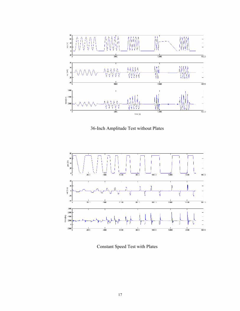
36-Inch Amplitude Test without Plates

Constant Speed Test with Plates

18

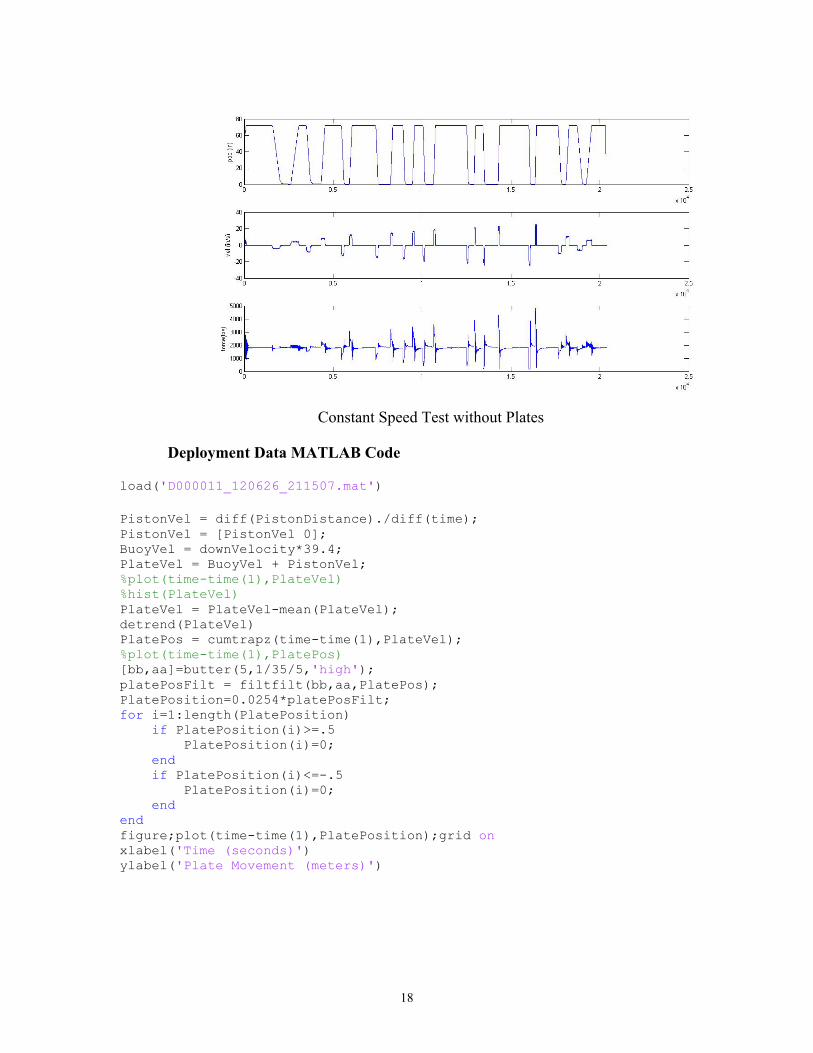
Constant Speed Test without Plates

Deployment Data MATLAB Code

load('D000011_120626_211507.mat') PistonVel = diff(PistonDistance)./diff(time); PistonVel = [PistonVel 0]; BuoyVel = downVelocity*39.4; PlateVel = BuoyVel + PistonVel; %plot(time-time(1),PlateVel) %hist(PlateVel) PlateVel = PlateVel-mean(PlateVel); detrend(PlateVel) PlatePos = cumtrapz(time-time(1),PlateVel); %plot(time-time(1),PlatePos) [bb,aa]=butter(5,1/35/5,'high'); platePosFilt = filtfilt(bb,aa,PlatePos); PlatePosition=0.0254*platePosFilt; for i=1:length(PlatePosition) if PlatePosition(i)>=.5 PlatePosition(i)=0; end if PlatePosition(i)<=-.5 PlatePosition(i)=0; end end figure;plot(time-time(1),PlatePosition);grid on xlabel('Time (seconds)') ylabel('Plate Movement (meters)')

19

Test data MATLAB code

close all clear all data = load('wPlates-A36-sin.csv'); %%"Inch","lbf","PSI","PSI","Volt","degC","degC","cm" dt = .04; t = data(:,1); pos = data(:,2); force = data(:,3); clear data; vel = [0; diff(pos)/dt]; idx = find(vel > 30); %Remove outliers due to starting and stopping logging. vel(idx) = 0; %Filter numerical derivatives to smooth. b = ones(1,8)/8; a = [1]; vel = filtfilt(b,a,vel); accel = [0; diff(vel)/dt]; idx = find(accel > 30); %Remove outliers due to starting and stopping logging. accel(idx) = 0; accel = filtfilt(b,a,accel); force = filtfilt(b,a,force); force = force-180; %Correct for weight of ram. fh = figure('Position',[6 38 1267 690]); ah1 = subplot(3,1,1) plot(pos) ylabel('pos (in)'); ah2 = subplot(3,1,2) plot(vel); ylabel('vel (in/s)'); ah3 = subplot(3,1,3) plot(force) ylabel('force(lbs)'); xlabel('time (s)'); linkaxes([ah1 ah2 ah3],'x'); start = [243 4100 9204 12480]; stop = [2867 6005 10160 13960];

20

idx = []; for i = 1:length(start) idx = [idx start(i):stop(i)]; end pos = pos*.0254; %Convert to meters. vel = vel*.0254; accel = accel*.0254; m = 2250/2.2; %Mass in kg g = 9.81; Area = 14.34; %plate area in m^2 rho = 1025; %water density V = .142; %volume of plate in m^3 F = force(idx)*4.45; %newtons A = [accel(idx) .5*rho*Area*vel(idx).*abs(vel(idx))]; B = F + rho*V*g - m*(accel(idx)+g); x = A\B; mu = x(1); Cd = x(2); Force = (m+mu)*accel(idx) + Cd*.5*rho*Area*vel(idx).*abs(vel(idx)) + m*g - rho*V*g; fh = figure('Position',[6 38 1267 690]); subplot(2,1,1) [ah1,h11,h12] = plotyy(t,pos/.0254,t,vel/.0254); %set(ah1(1),'YLim',[-1 1]); %set(ah1(1),'YTick',-1:2/8:1); set(ah1(2),'YLim',[-25 25]); set(ah1(2),'YTick',-25:50/10:25); set(get(ah1(1),'Ylabel'),'String','Position (in)'); set(get(ah1(2),'Ylabel'),'String','Vel (in/s)'); ah2 = subplot(2,1,2) plot(t(idx),force(idx),t(idx),Force/4.45); xlabel('seconds'); ylabel('force (lbs)'); legend('Measured Force',['Estimated Force: mu = ' num2str(mu,4) 'kg, Cd = ' num2str(Cd,2)],'Location','NorthWest');

linkaxes([ah1(1) ah1(2) ah2],'x');

21

22