improving the hydrodynamic performance of diffuser vanes ... · pdf fileimproving the...
TRANSCRIPT

Improving the Hydrodynamic Performance of
Diffuser Vanes via Shape Optimization
Tushar Goel' * , Daniel J Dorney2** , Raphael T. Haftka3* , and Wei Shyy4t
*Department of Mechanical and Aerospace Engineering, University of Florida,
Gainesville, FL 32611
**ER42, NASA Marshall Space Flight Center, AL 35812
tDepartment of Aerospace Engineering, University of Michigan, Ann Arbor, MI 48109
Abstract
The performance of a diffuser in a pump stage depends on its configuration and placement within the stage.
The influence of vane shape on the hydrodynamic performance of a diffuser has been studied. The goal of
this effort has been to improve the performance of a pump stage by optimizing the shape of the diffuser
vanes. The shape of the vanes was defined using Bezier curves and circular arcs. Surrogate model based
tools were used to identify regions of the vane that have a strong influence on its performance.
Optimization of the vane shape, in the absence of manufacturing. and stress constraints, led to a nearly nine
1 PhD Candidate, Student Member AIAA
2 Aerospace Engineer, Associate Fellow AIAA
3 Distinguished Professor, Fellow AIAA
4 Clarence L "Kelly" Johnson Professor, Fellow AIAA
1
https://ntrs.nasa.gov/search.jsp?R=20070032727 2018-05-11T13:36:49+00:00Z

percent reduction in the total pressure losses compared to the baseline design by reducing the extent of the
base separation.
Keywords: Diffuser, Multiple surrogates, shape optimization, hydrodynamics
1. Introduction
The space shuttle main engine (SSME) is required to operate over a wide range of
flow conditions. This requirement imposes numerous challenges on the design of
turbomachinery components. One concept that is being explored is the use of an expander
cycle for an upper stage engine. A schematic of a representative expander cycle for a
conceptual upper stage engine is shown in Figure 1. Oxidizer and fuel pumps are used to
feed LOX (liquid oxygen) and LH2 (liquid hydrogen) to the combustion chamber of the
main engine. The combustion products are discharged from the nozzle. The pumps are
driven by turbines, which use the gasified fuel as the working fluid.
There is a continuing effort to develop subsystems like turbopumps and turbines used
in a typical expander cycle based upper stage engine. The requirements on the design of
subsystems are influenced by size, weight, efficiency, and manufacturability of the
system. Besides, often the requirements for subsystems are coupled, for example, the
above-mentioned design constraints require turbopumps to operate at high speeds to have
high efficiency with low weight and compact design. This may "require seeking alternate
designs for the turbopumps as the current designs may not prove adequate over a wide
range of operating conditions. Mack et al. [1, 2] optimized the design of a radial turbine
that allows high turbopump speeds, performs comparable to an axial turbine at design
conditions, and yields good performance at off-design conditions.
2

Dorney et al. [3] have been exploring different concepts for turbopump design. A
simplified schematic of a pump is shown in Figure 2. Oxidizer or fuel enters from the
left. The pressure increases as the fluid passes through the impeller. The fluid emerging
from the impeller periphery typically has high tangential velocity, which is partially
converted into pressure by passing it over a diffuser. Dorney et al. [3] found that a
diffuser with vanes is more efficient than a vaneless diffuser at off-design conditions.
Over a range of operating conditions, the performance of a pump is driven by the flow in
the diffuser. Generally; the diffuser will stall before the impeller, and the performance of
the diffuser will drop off more rapidly at off-design operating conditions. The main
objectives of the current effort are to improve the hydrodynamic performance of a
diffuser, using advanced optimization techniques, and to study the features of the diffuser
vane that influences its performance.
Improvement in performance via shape optimization has been successfully achieved
in many areas. For example, there are numerous instances of improvement in lift to drag
ratio via airfoil or wing shape design [4-10], shape of blades is optimized to increase the
efficiency of turbines [4, 11] and pumps [12] in past. Shape design typically involves
optimization that requires a significant number of function evaluations to explore
different concepts. If the cost of evaluating a single design is high, as is usually the case,
surrogate models of objectives and constraints are frequently used to reduce the
computational burden.
Surrogate based optimization approach is widely used in the design of space
propulsion systems, such as radial turbines [1, 2], supersonic turbines [4], diffusers [13],
rocket injectors [14, 15], and combustion chamber geometry [16]. Detailed reviews on
3

surrogate based optimization are provided by Li and Padula [17] and Queipo et al. [18].
There are many surrogate models, and it is not clear which surrogate model performs the
best for any particular problem. In such a scenario, one possible approach to account for
uncertainties in predictions is to use an ensemble of surrogates (Goel et al. [19]). This
multiple surrogate approach has been demonstrated to work well for several problems
including system identification (Goel et al. [20]), compressor blade design (Samad et al.
[12])
Specifically, the objectives of the present study are: (i) to 'improve the hydrodynamic
performance of the diffuser via shape optimization of vanes, (ii) to identify important
regions in diffuser vanes that help optimize pressure ratio, and (iii) to demonstrate the
application of multiple surrogates based strategy for space propulsion systems.
The paper is organized as follows. We define the geometry of the vanes, and
numerical tools to evaluate the diffuser vane shapes in Section II. We describe the
relevant details in surrogate model based optimization in Section III. The results obtained
for the current optimization problem and a discussion of the physics involved in flow
over optimal vane is presented in Section IV. Finally, we conclude by recapitulating the
major findings of the paper in Section V.
2. Problem description
Representative radial locations in the meanline pump flow path (not-to-scale) are
shown in Figure 3 (Dorney et al. [3]). The fluid enters from the left, and is guided to the
unshrouded impeller via inlet guide vanes assembly. The flow from the impeller passes
through the diffuser before being collected in the discharge collector. In this study, we
focus our efforts on a configuration of 15 inlet guide vanes, seven main and seven splitter
4

blades, and 17 diffuser vanes. The length of the diffuser vanes is also fixed according to
the location of the collector. Our goal is to maximize the performance of the diffuser,
characterized by the ratio of pressure at the inlet and the outlet, hereafter called as
`pressure ratio'. The performance of the diffuser is governed by the shape of the diffuser
vane.
21. Vane shape definition
The description of geometry is the most important step in the shape optimization. The
current shape of the diffuser vanes, referred as baseline design, (shown in Figure 4(A))
was created using meanline and geometry generation codes at NASA [21] and yields a
pressure-ratio of 1.074. It is obvious from Figure 4(B) that the existing shape allows the
flow to remain attached while passing on the vanes but causes significant flow separation
while leaving the vane. The separation induces significant loss of pressure recovery that
is the primary goal of using a diffuser. The baseline design was created subject to several
constraints, including: i) the number of vanes was set at 17 based on the number of bolts
used to attach the two sides of the experimental rig, ii) the vanes had to accommodate a
3/8-inch diameter bolt, with enough excess material to allow manufacturing, and 'iii) the
length of the vanes was set based on the location of the collector. These constraints
resulted in an initial optimized design that looked quite similar to the baseline design, and
yielded similar performance in both isolated component and full stage simulations. In an
effort to more thoroughly explore the design space for diffusers (and allowing for future
improvements in materials and manufacturing), the constraints resulting from the bolts
(the number and thickness of the vanes) were relaxed. Other factors that must be
considered in the following optimization include: i) the designs resulting from the
5

optimization techniques shown in this paper are based on diffuser-alone simulations
(different results may be obtained if the optimizations were based on full stage
simulations), and ii) no effort was made to determine if the proposed designs would meet
stress and/or manufacturing requirements.
To reduce the separation, we represent the geometry of a vane by five sections using a
circular arc and Bezier curves as shown in Figure 5. Sections 1, 3, and 4 are Bezier
curves, and Section 2 is a circular arc. The shape of the inlet nose (between points B 1 and
B2) is obtained from the existing baseline vane shape. The circular arc in Section 2 is
described by fixing the radius r (r = 0.08), the location of the center Cl (-3.9, 6.1), the
start and end angles [21 ]. The arc begins at angle ;T + Or + 8 / 2 (point Al) and ends at
z + B — 6 / 2 (point A2). Here, we use B = 22.5° and 9 is a design variable. We provide
the information about the coordinates and slope of the tangents at endpoints such that
different Bezier curves (Appendix 1) are generated by varying the length of tangents. The
points AI and A2, shown by red dots in Figure 5, and the tangents to the arc, serve as the
end points location and tangents used to define the Bezier curves in Sections 1 and 3.
Coordinates and the slopes at points B 1 and B2 (obtained using the data of inlet nose of
the baseline design [21]) are used to define Bezier curves in Sections 1 and 4. The Bezier
curve in Section 1 (Figure 5) is defined using the coordinates and slope of tangents at B2
and A2. The lengths of the tangents tl and t2 control the shape of the curve. While one end
point coordinates and slope for Bezier curves in Sections 3 and 4 are known at points AI
and B 1 , the second end point and slope are obtained by defining the location of point P
(Py, PZ). The slope of tangent at point P is taken as five degrees more than the slope of the
line joining points P and B 1 . The additional slope is specified to avoid all the points in
6

Section 4 fall in a straight line. The values of the fixed parameters are decided based on
the inputs from designer [21]. The lengths of tangents tl-t6 serve as variables to generate
Bezier curves in Sections 1, 3 and 4.
The ranges of the design variables, summarized in Table 1, are selected such that we
obtain practically feasible vane geometries and the corresponding grids (discussed in next
section). We note that present Bezier curve and circular arc based definition of diffuser
vane shapes provides significantly' different vane geometries than the baseline design,
particularly near the outlet region. The main rationale behind this choice of vane shape is
the relaxation of manufacturing and stress constraints, ease of parameterization and better
control of the curvature of the vane that allows the flow to remain attached.
2.2. Mesh generation, boundary conditions, and numerical simulation
Performance of diffuser vane geometries is analyzed using' the NASA PHANTOM
code [22] developed at Marshall Space Flight Center to analyze turbomachinery flows.
This 3D, unsteady, Navier-Stokes code utilizes structured, overset O- and H-grids to
discretize and analyze the unsteady flow resulting from the relative motion of rotating
components. The code is based on the Generalized Equations Set methodology [23] and
utilizes a modified Baldwin-Lomax turbulence model [24]. The inviscid and viscous
fluxes are discretized using a third-order spatially accurate Roe's scheme, and second-
order central differencing, respectively. The unsteady terms are modeled using a second
order accurate scheme.
For this problem, we solve incompressible, unsteady, non-rotating, turbulent, single
phase, constant-material-property flow over diffuser vane. The working fluid is water. By
taking the advantage of periodicity, only a single vane is analyzed here. A combination of
7

H- and O-grids with 13065 grid points, has been used to analyze diffuser vane shapes. A
typical grid is shown in Figure 6. The boundary conditions imposed on the flow domain
are as follows. Mass flux, total temperature, and flow angles (circumferential and radial)
are specified at the inlet. Mass flux is fixed at the outlet. All solid boundaries are modeled
as no slip, adiabatic walls, with zero normal derivative of pressure. Periodic boundary
condition is enforced at outer boundaries. With this setup, it takes approximately 15
minutes on a single Intel Xeon processor (2.0 GHz, 1.0 GB RAM) to simulate each
design.
3. Methodology
As discussed earlier, the surrogate model based approach is suitable to reduce the
computational cost of optimization. In this section, we discuss different steps and
considerations in surrogate modeling and its application to the design problem(s). A
stepwise procedure of surrogate based analysis and optimization is explained with the
help of Figure 7. Firstly, we identify the objectives, constraints, and design variables.
Next, we develop a procedure to evaluate different designs. In context of the current
problem, we identified design variables, objectives, and numerical procedure to evaluate
different designs in the previous section. To reduce the computational expense involved
in optimization, we construct multiple surrogate models of the objectives and constraints.
A brief description of popular surrogate models is as follows.
3.1. Surrogate modeling
There are many surrogate models e.g., polynomial response surface approximations,
kriging, radial basis neural network, support vector regression etc. A detailed discussion
8

of different aspects of surrogate modeling was reviewed by Li and Padula [17] and
Queipo et al. [18]. We give a brief description of different surrogate models as follows.
3. I. I. Polynomial response surface approximation (PRS, [25])
The observed response y(x) of a function at point x is represented as a linear
combination of basis functions f(x) (mostly monomials are selected as basis functions)
and coefficients 8,. Error in approximation s is assumed to be uncorrelated and
normally distributed with zero mean and 62 variance. That is,
y(x) = 1 /jff (x) +s; E(E) = 0, V(6) = 62 (1)i
The polynomial response surface approximation of y(x) is,
Y(x) _ b, f (x), (2)
where bT is the estimated value of the coefficient associated with the iah basis function
fi(x). The coefficient vector b is obtained by minimizing ` the error in approximation
(e(x) = y(x) — y(x)) at NS sampled design points in a least square sense as,
b = (XT X) -' XT y, (3)
where X is the matrix of basis functions and y is the vector of responses at NS design
points. The quality of approximation is measures by computing the coefficient of
multiple determination R2 ; defined as,
2 2 (NS _ 1)
Radj = 1 — 6aNS— 2 ' (4)
Y(y'-y)i.1
9
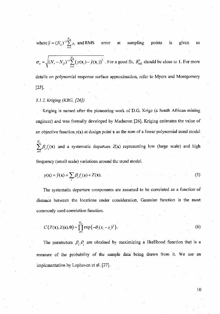
NS
where y= (N,)-
y, and RMS error at sampling points is given asi-1
NS
6Q = (NS — Nfl )_ 1
J (y(xi ) - y(x, ))2 . For a good fit, R a, should be close to 1. For morei=1
details on polynomial response surface approximation, refer to Myers and Montgomery
[25]
3.1.2. Kriging (KRG, [261)
Kriging is named after the pioneering work of D.G. Krige (a South African mining
engineer) and was formally developed by Matheron [26]. Kriging estimates the value of
an objective function y(x) at design point x as the sum of a linear polynomial trend model
N„
[3, f (x) and a systematic departure Z(x) representing low (large scale) and high
frequency (small scale) variations around the trend model.
Y(x) = Y(x) = ,13 f (x) + Z(x). (5)i
The systematic departure components are assumed to be correlated as a function of
distance between the locations under consideration. Gaussian function is the most
commonly used correlation function.
N„
C (Z(x), Z(s), 6) = fl exp (—B, (x, - s; ) 2 ) . (6)i=1
The parameters 83 , 01 are obtained by maximizing a likelihood function that is a
measure of the probability of the sample data being drawn from it. We use an
implementation by Lophaven et al. [27].
10

3.1.3. Radial basis neural network (RBNN, [28])
The objective function is approximated as a weighted combination of responses from
radial basis functions (also known as neurons).
NRBF
Y(x) _ w;a,{x), (7)
where ai(x) is the response of the ith radial basis function at design point x and w; is the
weight associated with a;(x). Mostly Gaussian function is used for radial basis function
a(x) as
a = radbas (s — x1l b); radbas (n) = e -n2 . (8)
The parameter b in the above equation is inversely related to a user defined parameter
"spread constant" that controls the response of the radial basis function. A higher spread
constant would cause the response of neurons to be very smooth and very high spread
constant would result into a highly non-linear response function. Typically, spread
constant is selected between zero and one. The number of radial basis functions (neurons)
and associated weights are determined by satisfying the user defined error "goal" on the
mean square error in approximation. The usual value of goal is the square of five-percent
of the mean response.
As discussed here, we have many surrogate models and it is unknown a priori, which
surrogate would be most suitable for a given problem. Besides, the choice of best
surrogate model changes with sampling density and nature of the problem [19]. It has
been shown by Goel et al. [19] that in such scenario simultaneously using multiple
surrogate models protects us from choosing wrong surrogates. They proposed using a
weighted averaged surrogate that is described as follows.
11

3.1.4. PRESS-based weighted average surrogate model (PWS, [19])
We develop a weighted average surrogate model as,
Nyp , (x) _ WISi (x), (9)
i
where y" (x) is the predicted response by the weighted average of surrogate models,
y; (x) is the predicted response by the i t' surrogate model and w, is the weight associated
with the iffi surrogate model at design point x. Furthermore, the sum' of the weights must
NsM
be one YI w; =1) so that if all the surrogates agree, y,' (x) will also be the same.i=1
Weights are determined as follows.
E
R
w*n,7 = 7 E + a , n';aVg
w' (10)N^
EQVg = E, NSM ; ,8 < 0, a < 1,
where Ei is the global data-based error measure for iih surrogate model. In this study,
generalized mean square cross-validation error (GMSE) (leave-one-out cross validation
or PRESS in polynomial response surface approximation terminology), defined in the
Appendix 2, is used as global data-based error measure, by replacing E by GMSE .
We use a= 0.05 and,8 = —1. The above mentioned formulation of weighting schemes is
used with polynomial response surface approximation (PRS), kriging (KRG) and radial
basis neural networks (RBNN) such that,
ypws = W prsyprs + Wkg ykg + W,-h.yrb.' (I 1)
12

For more details about the weighted average surrogate model, we refer the reader to Goel
et al. [ 19].
Next, we use these surrogate models to characterize the importance of different
variables and to identify the most and the least 'important variables for different
objectives and constraints. This information is vital to understand the role of the
variables. Also, we can fix the least important variables to reduce the dimensionality of
the problem. We use global sensitivity analysis method proposed by Sobol [29].
3.2. Global sensitivity analysis (GSA, [291)
Sobol [29] presented a variance based, non-parametric approach to perform global
sensitivity analysis. In this approach, the response function is decomposed into unique
additive functions of variables and their interactions such that the mean of each additive
function is zero. This decomposition allows the variance (V) to be computed as a sum of
individual partial variance of each variable (Vi) and partial variance of interactions (ViY) of
different variables. The sensitivity of the response function with respect to each variable
is assessed by comparing the sensitivity indices (Si, Sy) that is the relative magnitude of
partial and total variance of each variable. The details of the method are as follows.
A function Ax) of a square integrable objective as a function of a vector of
independent uniformly distributed random input variables, x in domain [0, 1] is assumed.
The function can be decomposed as the sum of functions of increasing dimensionality as
AX) = fO + EJi(xi) + Jfti( xi 1xj) +'. + J]2...N,(XIIX21...IX1,)1 (12)
i ki
where fa _ o
f d x. If the following condition
13

1
ff, ... t, A, =0, (13)0
is imposed for k = il, is, then the decomposition described in Equation (12) is unique.
In context of global sensitivity analysis, the total variance denoted as V(t) can be shown
equal to
Nv
V(f) V +, ( 14)i=1 1_<z,j<_Nv
where V(f) = E((f _ f0)2 ), and each of the terms in Equation (14) represents the partial
contribution or partial variance of the independent variables (Vi) or set of variables to the
total variance and provides an indication of their relative importance. The partial
variances can be calculated using the following expressions:
V = V (E[.f I xi ]),
Vj =V(E[.f I xi, x; ]>-V - Vj, (15)
Vjk =V(E[f I xi , xj,xj])-Vjj -Vk -Vjk -V - Vj -Vk,
and so on, where V and E denote variance and expected value respectively. Note that
E [ f I x;f,.dx,, and V(E[ f I x, ]) bl f ?dxi This formulation facilitates the
computation of the sensitivity indices corresponding to the independent variables and set
of variables. For example, the first and second order sensitivity indices can be computed
as
Under the independent model inputs assumption, the sum of all the sensitivity indices
is equal to one. The first order sensitivity index for a given variable represents the main
14

effect of the variable, but it does not take into account the effect of the interaction of the
variables. The total contribution of a variable to the total variance is given as the sum of
all the interactions and the main effect of the variable. The total sensitivity index of a
variable is then defined as
V+YV;+IIV;k+:..Stotal = J.J#i I, j#i k,k#i (17)
' V(f)
Note that the above referenced expressions can be easily evaluated using surrogate
models of the objective functions. Sobol [29] has proposed a variance-based non-
parametric approach to estimate the global sensitivity for any combination of design
variables using Monte Carlo methods. To calculate the total sensitivity of any design
variable xi, the design variable set is divided into two complementary subsets of xi and Z
(Z = x j , Vj =1, Nv ; j # i) . The purpose of using these subsets is to isolate the influence of
xi from the influence of the remaining design variables included in Z. The total sensitivity
index for xi is then defined as
S, total _ Vi total
( 18)t IV W I)'
where
Vi total = Vi +.Vi,Z ., (19)
where Vi is the partial variance of the objective with respect to x i and Vi z is the measure
of the objective variance that is dependent on interactions between x i and Z. Similarly, the
partial variance for Z can be defined as VZ. Therefore the total objective variability can be
written as
15

V = V, + VZ + Vt Z . (20)
While Sobol [29] had used Monte Carlo simulations to conduct the global sensitivity
analysis, we use Gauss-quadrature numerical integration of different partial variance
terms in Equation (15) to calculate sensitivity indices.
Surrogate models, which represent objectives and constraints, are used to optimize
the performance of the system. If we use multiple surrogates, we will find more than one
candidate optimal solutions. The performance- of such predicted optimal designs is
validated using numerical simulation. If we are satisfied with the performance of the
subsystem, we terminate the search procedure. Otherwise, we refine the design space in
the region of interest. The design space refinement can be done in multiple ways, (i) we
can fix the least important variables at the optimal values (as ,realized by optimization) or
mean values to reduce the dimensionality of the problem, (ii) we sample more points in
the design space, and (iii) we identify the region where we expect potential improvement
and concentrate on that region. We repeat this optimization procedure till convergence.
4. Results and discussion
We present application of the above-mentioned surrogate based optimization
framework to optimize the performance of diffuser vanes in this section. We also present
a detailed analysis of optimal design.
4.1. Surrogate model construction
First step in surrogate modeling is to sample data in design variable space. Different
design of experiment (DOE) techniques are effective in reducing _ the computational
expense of generating high-fidelity surrogate models. The most popular methods DOE
16

methods are Latin hypercube sampling (LHS) and face-centered central composite
designs (FCCD). The choice of DOE depends on the nature of problem and the number
of samples required.
For this problem, we have nine design variables hence we selected 110 design points
to allow adequate data to evaluate 55 coefficients of a quadratic polynomial response
surface. Since face-centered central composite design requires unreasonably large
number of samples (531 points to approximate 55 coefficients), we use Latin hypercube
sampling (LHS) to construct surrogate models. We generated LHS designs using Matlab
routine `lhsdesign' with 100 iterations for maximize the minimum distance between
points. We evaluated each diffuser vane shape using PHANTOM. This dataset is referred
as `Set A'. The range of the data, given in Table 2, indicated potential of improvement in
the performance of the diffuser by shape optimization. We constructed four surrogate
models, polynomial response surface approximation (PRS), kriging (KRG), radial basis
neural network (RBNN), and PRESS-based weighted average surrogate (PWS) of the
objective pressure ratio. We used quadratic polynomial for PRS, and linear trend model
with Gaussian correlation function for kriging. For RBNN, the spread coefficient was
taken as 0.5 and the error goal was the square of 5% of the mean value of the response at
data points. The parameters a, and,8 for PWS model were 0.05 and -1, respectively. The
summary of quality indicators for different surrogate models is given in Table 2.
All error indicators are desired to be low compared to the response data, except R d, ,
which is desired to be close, to one. The PRESS (Appendix 2) and RMS error (-1.0e-2)
were very high compared to the range of data. This indicated that all surrogate models
poorly approximated the actual response, and were likely to yield inaccurate results if
17

used for global sensitivity analysis and optimization. To identify the cause of poor
surrogate modeling, we conducted a lack-of-fittest (refer to Appendix.3) for PRS. A low
p-value (0.017) indicated that the chosen order of the polynomial was inadequate in the
selected design space. Since, the data available at 110 points is insufficient to estimate
220 coefficients in a cubic polynomial, this issue of model inadequacy also reflected lack
of data.
4.2. Design space refinement
We addressed the issue of model accuracy or data inadequacy using two parallel
approaches. Firstly, we added more data in the design space to improve the quality of fit.
We sampled 330 additional points using Latin hypercube sampling such that we had 440
design points to fit a cubic polynomial (220 coefficients). We call this dataset as `Set B'.
Secondly, the low mean value of the response data (1.041) at 110 points compared to the
baseline design (1.074) indicated that large portion of the current design space was
undesirable due to inferior performance. Hence, it might be appropriate to identify the
region where we expect improvements in the performance of the designs, and construct
surrogate models by sampling additional design points in that region (reasonable design
space approach [31]). To identify the region of interest, we used the surrogate models,
constructed with Set A data (110 design points), to evaluate response at a large number of
points in design space. Specifically, we evaluated responses at a grid of four Gaussian
points in each direction (total 4 9=262,144 points). We chose Gaussian points instead of
usual uniform grids because Gaussian points lie inside the design domain, and -are less
susceptible to extrapolation errors than corners of uniform grids that might fall outside
the convex hull of LHS design points used to construct surrogate models. Any point with
18

a predicted performance (due to any surrogate model) of 1.08 units . or better (0.5%o
improvement over the baseline design) was considered to belong to the potential region
of interest. This process identified 29,681 unique points (-11%) in the potential good
region. We selected 110 points from this data set using D-optimality criterion in this
smaller region. D-optimal designs were generated using Matlab routine `candexch' with a
maximum of 100 iterations to maximize D-efficiency ([25], pp. 93). This 110 points
dataset is called `Set C'.
As before, we conducted simulations at data points in the Sets B and C ,using
PHANTOM. One point in each set failed to provide an appropriate mesh. The mean,
minimum, and maximum values of the pressure ratio for the two datasets are summarized
in Table 3. We observed only minor differences in the mean pressure-ratio of the Set B
compared to the Set A (Table 2) but the responses in the Set C data clearly indicated high
potential of improvement. This demonstrates the effectiveness of reasonable design space
approach used to identify the region of interest.
We approximated the data in the Set B and the Set C using four surrogates. We
employed a reduced cubic, and a reduced quadratic polynomial for PRS approximation of
the Set B and the Set C data, respectively. As can be seen from different error measures
in Table 3, the quality of surrogate models fitted to the Set B and the Set C data was
significantly better than the surrogate models fitted to the Set A data. This improvement
in surrogate approximation was attributed to the increase in the sampling density (Set B)
allowing a cubic model and the reduction of the design space (Set Q. Both PRS models
did not fail the lack-of-fit test (p-value —0.90+) indicating the adequacy of fitting
surrogate model in the respective design spaces. The PRESS metric and weights
19

associated with different surrogates suggested that the PRS was the best surrogate model
for the Set B and the Set C data, unlike kriging for the Set A data.
We used the surrogate models fit to the Set B data for global sensitivity analysis and
the surrogate models fitted to the Set C data for optimization. The optimization of the
performance using the surrogate models fitted to the Set B data was inferior to the
optimal design obtained using the Set C data based surrogates. Some of the optimal
designs from the Set B data based surrogates could not be analyzed. This anomaly arose
because large design space was sampled with limited data such that large regions remain
unsampled; and hence, susceptible to significant errors, particularly near the corners
where optima were found. The same issue restricted the use of surrogate models
constructed using Set C data for global sensitivity analysis as there is large extrapolation
error outside the region of interest where no point was sampled. Hence, surrogate models
constructed using Set B data were more suited for conducting global sensitivity analysis.
4.3. Global sensitivity assessment
We used global sensitivity analysis (GSA) to identify the most and the least important
design variables. We used Gauss quadrature numerical integration scheme with four
Gauss points along each direction (total 49=262,144 points) to evaluate different integrals
in GSA. The response at each point was evaluated using surrogate models fit . to the Set B
data. Corresponding sensitivity indices of main effects of different variables are shown in
Figure 8. Though there are differences in the exact magnitude of sensitivity indices from
various surrogates, all surrogates indicated that the pressure ratio was most influenced by
three variables, PZ, t2, and Py. A comparison of sensitivity indices of total and main effect
20

of design_ variables (using PWS) in Figure 9 suggested that the interactions between
variables are small but non-trivial.
4.4. Validation of global sensitivity analysis results
To validate the findings of the global sensitivity analysis, we evaluated the variation
in the response function (pressure ratio) by varying one variable at a time while keeping
remaining variables at the mean values. We specified five equi-spaced levels for each
design variable and used trapezoidal rule to compute the actual variance. The responses at
design points were evaluated by performing actual numerical simulations. The results of
actual variance computations are shown in Figure 10.
The one-dimensional variance computation results also indicated that variables PZ, t2,
and Py were more important than all other variables. This validated the findings of the
global sensitivity analysis. The differences in the results of one-dimensional variance
computation and global sensitivity analysis can be explained as follows: (i) the number of
points used to compute one-dimensional variance is small, (ii) one-dimensional variance
computation does not account for interactions between variables, and (iii) there are
approximation errors in using surrogate models for global sensitivity analysis.
Nevertheless, the main implications of the finding clearly show that the performance of
the diffuser vane was pre-dominantly affected by the location of point P and the length of
tangent t2 in Section 1 (Figure 5).
4.5. Preliminary optimization of diffuser vane performance
Next, we used surrogate models, fit to the Set C data, to maximize the pressure-ratio
by exploring different diffuser vane shapes. To avoid the danger of large extrapolation
errors in the unsampled region, we employed the surrogate model (PRS surrogate) from
21

the Set A as a constraint (all points in the feasible region have predicted response greater
than a threshold value of 1.08). Our use of PRS from the Set A as the constraint was
motivated by the simplicity of the constraint function, and the fact that PRS contributed
to the most number of points in the potential region of interest.
We used sequential quadratic programming optimizer to find the optimal shapes. The
optimal configuration of blade shapes obtained using different surrogate models as
function evaluators is shown in Figure 11, and the corresponding optimal design
variables are given in Table 4. The optimal designs obtained from all surrogates were
close to each other in both function and design space. A few minor differences were
observed in relatively insignificant design variables (refer to the results of global
sensitivity analysis). Notably all design variables touched the bounds for PRS and were
close to the corner for other surrogate models. The small value of 0 indicated sharper
nose, as was used in the baseline design. Also, most tangents were at their lower bounds
that resulted in low curvature sections. Near the point P, the tangents were on their upper
limits to facilitate gradual transition in the slope. The optimal vane was thinner in the
middle section and was longer compared to the baseline design (Figure 11). The central
region of the optimal design was non-convex compared to the convex section for the
baseline design.
We simulated all four candidate optimal designs from different surrogate models to
evaluate the improvements. The actual and predicted performances from different
surrogates are compared in Table 5. We observed that the error in approximation for
different surrogates was comparable to their respective PRESS errors. Nevertheless, PRS
was the most accurate surrogate model and furnished the best performance shape. RBNN
22

was the worst surrogate model. PRESS-based weighted average surrogate model
performed significantly better than the worst surrogate. The best predicted diffuser vane
yielded significant improvements in the performance (1.117) compared to the baseline
design (1.074). We refer to this design as `intermediate optimal' design.
It is obvious that the design space refinement in the region of interest based on
multiple surrogates has pay-offs in the improved performance . of surrogates and the
identification of optimal design. The high confidence in the optimal predictions was also
derived from the similar performance of all surrogate models. The results also showed the
incentives (protection against the worst _design, proper identification of the reasonable
design space) of investing a small amount of computational resources in constructing
multiple surrogate models (less than the cost of a single simulation) for computationally
expensive problems, and then the extra cost of evaluating multiple optima.
We compared instantaneous (at the end of simulation) and time-averaged flow fields.
from the intermediate optimal design (from PRS) with the baseline design in Figure 12.
The intermediate optimal design allowed smoother turning of the flow compared to the
baseline design, and reduced the losses due to separation of the flow, which were
significantly high in the baseline design. Consequently, the pressure at the outlet was
higher for this intermediate optimal design. We also noted the increase in pressure on the
vane for the intermediate optimal design.
4.6. Design space refinement via dimensionality reduction
We used first design space refinement by identifying the region of interest. This
helped in identifying the intermediate optimal design. Since most design variables in the
optimal design were at the boundary of the design space (Table 4), further improvements
23

in the performance of the diffuser might be obtained by refining the design space. To
reduce the computational expense, we reduce the design space by utilizing the findings of
the global sensitivity analysis. We fixed six relatively insignificant design variables at the
optimal design (predicted using PRS), and expanded the range of the three most
important design variables. The modified ranges of the design variables and the fixed
parameters are given in Table 6. We selected 20 design points using a combination of
face-centered central composite design (15 points FCCD), and LHS designs (5 points) of
experiments. The range of pressure ratio at 20 design points is given in Table 7. Note that
all the tested designs in the refined design space perform better than the intermediate
optimal design.
As before, we constructed four surrogate models in the refined design space. The
performance metrics, specified in Table 7, indicated that all surrogate models
approximated the response function very well. The weights associated with different
surrogate models, suggested that a quadratic PRS approximation represents the data the
best. This result is not unexpected since any smooth function can be represented by a
second order polynomial if the domain of application is small enough. As before, PWS
model was comparable to the best surrogate model.
4.7. Final optimization
The. design variables for the four optimal designs of the diffuser vane obtained using
different surrogate models and corresponding surrogate-predicted and actual (CFD
simulation) pressure ratio are listed in Table 8. The error in predictions of surrogate
models compared well with the quality indicators and all surrogate models had only
minor differences in the performance. Also, the optimal vane shapes from different
24

surrogates were similar. In this case also, polynomial response surface approximation
conceded the smallest errors in prediction. While the performance of the optimal diffuser
vane has improved compared to the intermediate optimal design (compare to Table 5),
the contribution of the optimization process was insignificant. One of the data points (t2 =
0. 60, Py -2.00, PZ = 6.00) resulted in a better performance (P-ratio = 1.151) than the
predicted optimal. This result was not surprising because the optimal design existed at a
corner that was already sampled leaving little scope for further improvement.
Nevertheless, the optimizers correctly concentrated 'on the best region. As expected, the
optimized design is thinner and streamlined to further reduce the losses, and to improve
the pressure recovery. We analyzed the optimal diffuser vane shape according to the flow
structure and the other considerations as follows.
4.8. Flow structure
The instantaneous and time-averaged pressure contours for the optimal vane shape
(best data point) are shown in Figure 13. We observed further reduction in separation
losses, and smoother turning of the flow compared to the intermediate optimal design
obtained before design space refinement (Table 5). Consequently, the pressure rise in the
diffuser was higher. The optimal vane shape had a notable curvature in the middle section
on the lower side of the vane (near the point P). This curvature decelerated the flow and
led to faster increase in pressure (notice the shift of higher pressure region towards the
inlet in Figure 12 and Figure 13).
4.9. Vane loadings
The shapes and pressure loads on the baseline, intermediate optimal, and final optimal
vanes are shown in Figure 14. We noted the increase in the mean pressure on the diffuser
25

vane for the optimal design. The pressure loads near the inlet tip, and the pressure loading
on the diffuser vane, given by the area bound by the pressure profile on the two sides, had
reduced by optimization. However, the optimized diffuser vane might be susceptible to
high stresses as the optimal design was thinner compared to the baseline vane. The
intermediate optimal design served as a compromise design with relatively higher
pressure ratio (^-4%) compared to the baseline design and lower pressure loading on the
vanes compared to the optimal design.
In the future, this problem would be studied by accounting for manufacturing and
structural considerations like, stresses in the diffuser vanes. One can either specify a
constraint to limit stress to be less than the feasible value or alternatively, one can solve a
multi-objective optimization problem with two competing objectives, minimization of
stress or pressure loading in the vane, and maximization of pressure ratio.
4.10. Empirical considerations
Typically, the vane shape design is carried out using empirical considerations on the
gaps between adjacent diffuser vanes as shown in Figure 15. The empirical suggestions
on the ratio of different gaps [32] and actual values obtained for different vanes are given
in Table 9. Contrary to the empirical relations, the ratio of length to width gap (L/Wl),
and ratio of width gaps (W2/WI ) decreased as the pressure ratio increases, though the
actual magnitude of length and width of the gaps increase. The discrepancies between the
optimal design and the empirical optimal ratios [32] are explained by multiple design
considerations used for the empirical optimal. Firstly, we note that the optimization was
carried out for a 2D diffuser vane not for the combination of vanes and flow for which
empirical ratios are provided. This allowed a variable height of the vane for optimization.
26

However, the empirical ratios are obtained by assuming a constant channel height so that
the area ratio of the channel reduces to the ratio of width gaps (W2/WI ). Nevertheless,
this requires further investigation to understand the cause of discrepancies between
empirical ratios and that obtained for optimal design.
5. Summary
We used surrogate model based optimization strategy to maximize the hydrodynamic
performance of a diffuser, characterized by the increase in pressure ratio, by modifying
the shape of the vanes. The shape of the diffuser vanes was defined by a combination of
Bezier curves and a circular arc. Firstly, we defined the shape of the vane using nine
design variables and used surrogate models to represent the pressure ratio. We used lack-
of-fit test to identify the issues of model inadequacy, and insufficiency of the data to
represent the pressure ratio. We addressed these issues by, (i) adding more data points,
and (ii) identifying the region of interest using the less-accurate surrogate models. More
samples were added in the region of interest using the information from multiple
surrogate models.
The surrogate models, constructed with increased data and/or in smaller design space,
were significantly more accurate than the initial surrogate models. Also, during the
course of design space refinement, the best surrogate model changed from kriging (initial
data) to polynomial response surface approximation (all subsequent results). Had we
followed the conventional approach of identifying the best surrogate model with the first
design of experiments, and then using that surrogate model for optimization, we might
have not captured the best design. Thus, we can say that the results reflect the
27

improvements in the performance using the design space refinement approach, and using
multiple surrogates constructed by incurring a low computational cost.
We conducted a surrogate model based sensitivity analysis to identify the most
important design variables in the entire design space. Three design variables controlling
the shape of the upper and lower side of the vane were found to be most influential. We
used surrogate model in the reduced design space to identify the optimal design in nine
variable design space. This intermediate optimal design improved the pressure ratio by
more than four percent compared to the baseline design.
Since all the design variables for intermediate optimal design hit the bounds, we
further refined the design space by fixing the least important variables on optimal values
to reduce the design space, and relaxing the bounds on the most important design
variables. The optimal design obtained using the surrogate models in the refined design
space further improved the performance of the diffuser by more than seven percent
compared to the baseline design. The pressure losses in the flow were reduced, and a
more uniform pressure increase on the vane was obtained. However, the optimal vane
shape might be susceptible to fail due to high stresses. This behavior was attributed to the
absence of stress constraint that allowed using thinner vanes to maximize the
performance. In the future, the optimization would be carried out by considering the
multi-disciplinary analysis accounting for stress constraint, manufacturability, and
pressure increase.
In terms of the vane shapes, thin vanes helped improve the hydrodynamic
performance significantly. The interesting aspect was the change in the sign of curvature
28

of the vane on the suction side that allows an initial speeding of the flow followed by a
continuous pressure recovery without flow separation.
6. Acknowledgements
The present efforts have been supported by the Institute for Future Space Transport,
under the NASA Constellation University Institute Program (CUIP), Ms. Claudia Meyer
program monitor. This material is based upon work supported by the National Science
Foundation under Grant No. 0423280.
Appendix 1: Bezier Curve
A typical parametric Bezier curve f(x), shown in Figure 16, is defined with the help of
two end points Po and Pl, and two control points P2 and P3 as follows.
f (x) = P (1- x)3 +3Px(1- x)2 + 3P x2 (1- x) + Px3 , x E [0, 1]. (21)
The co-ordinate of any point on the Bezier curve is obtained by substituting the value
of x accordingly. In this study, the location of control points is obtained by using the
information about the slope and the length of the tangents at end points (Papila et al. [4]).
Appendix 2: Generajized Mean Square Cross-Validation Error (GMSE or PRESS)
In general, the data is divided into k subsets (k-fold cross-validation) of
approximately equal size. A surrogate model is constructed k times, each time leaving out
one of, the subsets from training, and using the omitted subset to compute the error
measure of interest. The generalization error estimate is computed using the k error
measures obtained (e.g., average). If k equals the sample size, this approach is called
leave-one-out cross-validation (also known as PRESS in the polynomial response surface
29

approximation terminology). Equation (22) represents_a leave-one-out calculation when
the generalization error is described by the mean square error (GMSE)
k
GMSE = _I (Y; '^) 2 , (22)
k ;_l
where represents the prediction at x( ' ) using the surrogate constructed using all
sample points except (x(O , yz ). Analytical expressions are available for that case for the
GMSE without actually performing the repeated construction of the surrogates for both
polynomial response surface approximation (Myers and Montgomery [25], Section 2.7)
and Kriging (Martin and Simpson [30]) however here we used brute-force. The
advantage of cross-validation is that it provides nearly unbiased estimate of the
generalization error and the corresponding variance is reduced (when compared to split-
sample) considering that every point gets to be in a test set once, and in a training set k-1
times (regardless of how the data is divided).
Appendix 3: Lack-of-Fit Test With Non-replicate Data for Polynomial ResponseSurface Approximation
A standard lack-of-fit test is a statistical tool to determine the influence of bias error
(order of polynomial) on the predictions [25]. The test cor'Apares the estimated
magnitudes of the error variance and the residuals unaccounted'' for by the fitted model.
Lets say, we have M unique locations of the data and at jth' location, we repeat the
experiment nj times, such that total number of points used to construct surrogate model is
M
N = in . The sum of squares due to pure error is given by,1=1
n2
SS Pe = I I (Y;k Y1)(23)
1=1 k=1
30

where –. is the mean response at the 'th sample location given as _
1 YiYJ p J p g Yj =—Ykn j
The sum of square of residuals due to Tack-of-fit of the polynomial response surface
model is,
M 2ssof = In j (Axj) —'yj) (24)j=1
where y(xj) is the predicted response at the sampled location x In matrix form, the
above expressions are given as,
MSS T I – '
IT,
(25
Pe " ^ yn n. n nJ n.^Y nl )
j=1 i j
M 1SSlof = yT ( N - X(XTX)-1 XT )y-1 Yn.
InJ n in. ln. yn ' (26)
j=1 i J
where 1n j nj J
is the (n x 1) vector of ones, I is (n . x n J . Ns
) identity matrix, I isJ
(Ns x Ns ) identity matrix.
We formulate F-ratio using the two residual sum of squares as,
F = (SS
lof I dlof)(SS /d (27 )
Pe pe
where dlof = N - N , and d Pe = NS M , are the degrees of freedom associated with
SS,O f and SSpe , respectively. The lack-of-fit in the surrogate model-is detected with a-
level of significance, if the value of F in Equation (27), exceeds the tabulated Fa,dlof' pe
value, where the latter quantity is the upper 100a percentile of the central F-distribution.
31

When the data is obtained from the numerical simulations, the replication of
simulations does not provide an estimate of noise (SSpe), since all replications return
exactly the same value. In such scenario, the variance of noise can be estimated by
treating the observations at neighboring designs as "near" replicates ([33], pp. 123). We
adopt the method proposed by Neill and Johnson [34], and Papila [35] to estimate the
lack-of-fit for non-replicate simulation. In this method, we denote a near-replicate design
point xjk (as the e replicate of the /h point xi ) such that
X .Jk ^ ^=X. .k+6 , (28)
where 6,k represents the disturbance vector. Then, the Gramian matrix is written as
X = X + 0,, (29)
where X matrix is constructed using ac i for near replicate points and matrix 0 = X —X .
Now the estimated response at the design points (including near-replicates) is given as
y = y - Ob, (30)
where b is given in Equation (3). Now, we compute SSpe and SSlof by replacing y, yn
and X in Equations (25) and (26) with y, yn and X.
32

7. References
1.Mack Y, Goel T, Shyy W, Haftka RT, Surrogate model based optimization
framework: A case study in aerospace design. In: Yang S, Ong YS, Jin Y, editors.
Evolutionary Computation in Dynamic and Uncertain Environments. Springer Kluwer
Academic Press, 2005.
2. Mack Y, Shyy W, Haftka RT, Griffin L, Snellgrove L, Huber F, Radial turbine
preliminary aerodynamic design optimization for expander cycle liquid rocket engine.
In: 42nd AIAA/ASME/SAE/ASEE joint propulsion conference and exhibit, Sacramento
CA, 9-12 July, 2006; AIAA-2006-5046.
3.Dorney DJ, RothermelJ,"Griffin LW, Thornton RJ, Forbes JC, Skelley SE, Huber FW,
Design and analysis of a turbopump for a conceptual expander cycle upper-stage
engine. In: Symposium of advances in numerical modeling of aerodynamics and
hydrodynamics in turbomachinery, Miami FL, 17-20 July, 2006; FEDSM2006-98101.
4. Papila N, Shyy W, Griffin L, Dorney DJ, Shape optimization of supersonic turbines
using global approximation methods. Journal of Propulsion and Power. 2002; 18(3):
509-518.
5.Obayashi S, Sasaki D, Takeguchi Y, Hirose N, Multi-objective evolutionary
computation for supersonic wing-shape optimization. IEEE Transactions on
Evolutionary Computation. 2000; 4(2): 182-187.
6. Sasaki D, Obayashi S, Sawada K, Himeno R, Multi-objective aerodynamic
optimization of supersonic wings using Navier-Stokes equations. In: European
33
congress on computational methods in applied sciences and engineering (ECCOMAS),
Barcelona Spain, September, 2000.
7. Sasaki D, Morikawa M, Obayashi S, Nakahashi K, Aerodynamic shape optimization
of supersonic wings by adaptive range multi-objective genetic algorithms. In: 1St
international conference on evolutionary multi-criterion optimization, Zurich, March,
2001; pp 639-652.
8.Huyse L, Padula SL, Lewis RM, Li W, Probabilistic approach to free-form airfoil
shape optimization under uncertainty. AIAA Journal, 2002; 40(9):.1764-1772.
9.Giannakoglou KC, Design of optimal aerodynamic shapes using stochastic
optimization methods and computational intelligence. Progress in Aerospace Sciences,
2002; 38: 43-76.
10.Emmerich MJ, Giotis A, Ozdemir M, Back T, Giannakoglou K, Metamodel-assisted
evolutionary strategies. In Parallel problem solving from nature VII conference,
Granada Spain, September, 2002; pp 361-370.
11.Mengistu T, Ghaly W, Mansour T, Global and local shape aerodynamic optimization
of turbine blades. In: Il th multidisciplinary analysis and optimization conference,
Portsmouth VA, 6-8 September, 2006; AIAA-2006-6933.
12. Samad A, Kim K-Y, Goel T, Haftka RT, Shyy W, Shape optimization of
turbomachinery blade using multiple surrogate models. In: Symposium of advances in
numerical modeling of aerodynamics and hydrodynamics in turbomachinery, Miami
FL, 17-20 July, 2006; FEDSM 2006-98368.
13.Madsen JI, Shyy W, Haftka RT, Response surface techniques for diffuser shape
optimization. AIAA Journal, 2000; 38(9): 1512-1518.
34

14.Vaidyanathan R, Papila N, Shyy W, Tucker KP, Griffin LW, Haftka RT, Fitz-Coy N,
Neural network and response surface methodology for rocket engine component
optimization. In: 8' AIAA/USAF/NASA/ISSMO symposium on multidisciplinary
analysis and optimization conference, Long Beach CA, 6-8 September, 2000; AIAA-
2000-4480.
15. Goel. T, Vaidyanathan R, Haftka RT, Shyy W, Queipo NV, Tucker KP, Response
surface approximation of Pareto optimal front in multi-objective optimization.
Computer Methods in Applied Mechanics and Engineering, doi
10.1016/j . cma.2006.07.010.
16.Mack Y, Goel T, Shyy W, Haftka RT, Queipo NV, Multiple surrogates for shape
optimization for bluff-body facilitated mixing. In: 43 rd AIAA aerospace sciences
meeting and exhibit, Reno NV, 10-13 Jan, 2005; AIAA-2005-0333.
17.Li W, Padula S, Approximation methods for conceptual design of complex systems.
In: Chui C, Neaumtu M, Schumaker L, editors. Approximation Theory XI: Gatlinburg,
Nashboro Press, Brentwood TN, 2005; pp 241-278.
18. Queipo NV, Haftka RT, Shyy W, Goel T, Vaidyanathan R, Tucker KP, Surrogate-
based analysis and optimization. Progress in Aerospace Sciences, 2005; 41: 1-28.
19. Goel T, Haftka RT, Shyy W, Queipo NV, Ensemble of surrogates. Structural and
Multi-disciplinary Optimization Journal, doi 10.1007/s00158-006-0051-9 (a different
version was presented at 11' AIAA/ISSMO multidisciplinary analysis and
optimization conference, Portsmouth VA, 6-8 September, 2006; AIAA-2006-7047).
20. Goel T, Zhao J, Thakur SS, Haftka RT, Shyy W, Surrogate model-based strategy for
cryogenic cavitation model validation and sensitivity evaluation. In: 42"d
35

AIAA/ASME/SAE/ASEE joint propulsion conference and exhibit, Sacramento CA, 9-
12 July, 2006; AIAA-2006-5047.
21. Dorney DJ, Personal communications. 2006.
22. Dorney DJ, Sondak DL, PHANTOM: Program user's manual. Version 20, April
2006.
23. Sondak DL, Dorney DJ, General equation set solver for compressible and
incompressible turbomachinery flows. In: 39th AIAA/ASME/SAE/ASEE joint
propulsion conference and exhibit, Huntsville AL, 20-23 July, 2003; AIAA-2003-4420.
24. Baldwin BS, Lomax H, Thin layer approximation and algebraic model for separated
flow. In: 16"' aerospace sciences meeting, Hunstville AL, 16-18 January, 1978; AIAA-
1978-257.
25. Myers RH, Montgomery DC, Response Surface Methodology, John Wiley and Sons,
Inc 1995.
26. Matheron G, Principles of geostatistics. Economic Geology, 1963; 58: 1246-1266.
27. Lophaven SN, Nielsen HB, Sondergaard J, DACE: A Matlab kriging toolbox.
Version 2,0, Information and mathematical modeling, Technical University of
Denmark, 2002.
28. Orr MJL, Introduction to radial basis function networks. Center for cognitive
science, Edinburg University, EH 9LW, Scotland UK. 1996,
hitp://www.anc.ed.ac.uk/—mjo/rbf.html.
29. Sobol IM, Sensitivity analysis for ' nonlinear mathematical models. Mathematical
Modeling & Computational Experiment, 1993; 1(4): 407-414.
36

30. Martin JD, Simpson TW, Use of kriging models to approximate deterministic
computer models. AIAA Journal, 2005; 43(4): 853-863.
31. Balabanov VO, Giunta AA, Golovidov O, Grossman B, Mason WH, Watson LT,
Haftka RT, Reasonable design space approach for response surface approximation.
Journal of Aircraft, 1999; 36(1): 308-315.
32. Stepanoff AJ, Centrifugal and Axial Flow Pumps, 2n d Edition, Krieger Publishing
Company, Malabar FL, 1993.
33. Hart JD, Non-parametric Smoothing and Lack of Fit Tests, Springer-Verlag,
NewYork, 1997.
34.Neill JW, Johnson DE, Testing linear 'regression function adequacy without
replications. The Annals of Statistics, 1985; 13(4): 1482-1489.
35. Papila M, Accuracy of Response Surface Approximations for Weight Equations
Based on Structural Optimization, PhD Thesis, The University of Florida, 2002.
37

O.daw Pumpfins %rbm foes Pump
Ww
Figures
N-1l
Figure 1 A representative expander cycle used in the upper stage engine (courtesy wikipedia).
Splitber Diffuserblade .—vane
Inlet guidevane Main impeller
bladeFigure 2 Schematic of a pump.
1
Main/Splitter' G
IGVblade
Figure 3 Meanline pump flow path (IGV: Inlet guide vane).
38

68
66
6.4
6.2
6
58
56
8
7
6
RHO
50002000900060.003000000070.0040.00
8
7
6
a.4 -4 -2 0
-5 -4 -3 -2 -1 0 1
(A) Shape of the diffuser vane (B) Streamlines and time-averaged pressure
Figure 4 Baseline diffuser vane shape and time-averaged flow.
Figure 5 Definition of the geometry of the diffuser vane (refer to Table 1 for variable description).
Figure 6 A combination of H- and 0-grids to analyze diffuser vane. Body-fitted 0-grids are shown ingreen and algebraic H-grid is shown in red.
39

t5
1.0%
r°
Define optimizationproblem
MhIAXII ,X2 .... X.)e.t C(z) < 0
H(z) = 0
Evaluate,4x),C(Y), H(x)
sr f
12 Surrogate H
models C
Refine designspace
Identify most andleast important Perform Vavariables using optimization
GSA
Figure 7 Surrogate based design and optimization procedure.
t, t2 t3 t4
0.4% 11.7%0.5°/6 ^0.1% tfi
0.4% \ 0.1%
t6
.1%
P"P2
6.8%79.8%
60.8%
P,
79.1'
Stop 1
t, t2
iL0.2% 13.1% t3
0.9% t40.0%
t5
0.0%
t6
0.0%
Py
6.0%
(A) Polynomial response surface
t, t21.00/o 12.9% t3
6 1.5%l.3% to
1 F0.9%
F
72.
(B) Kriging
t,
t2 t0.3%_\ 12.5% 3n aoi to
t5
0.1%
6
1%
(C) Radial basis neural network (D) PRESS-based weighted average
Figure 8 Sensitivity indices of main effect using various surrogate models (Set B).
40

Pz
Py
t6
d t5
t4
t3
t2
t1
E)
t 1t26
0.7% 20.3%
0.6%^ , 1t3
0.8% t4
0.4%
t5
0.0%
P 0.2%Y
13.7%
Pz
63.2%
0.00 0.20 0.40 0.60 0.80 1.00
Sensitivity index
Figure 9 Sensitivity indices of main and total effects of different variables using PWS (Set B).
Figure 10 Actual partial variance of different design variables (no interactions are considered).
Figure 11 Baseline and optimal diffuser vane shape obtained using different surrogate models. PRSindicates function evaluator is polynomial response surface, KRG stands for kriging, RBNN is radialbasis neural network, and PWS is PRESS -based weighted surrogate model as function evaluator.
41

RHO12
07 8
1.03
0.98
0.31
0 89084080 70.75
6
8
7
6
RHO
50.0020.0090 0060.0030.0000.E70.03
40.00
6 6
PH
12
07 8
1030880910690a1060075 7
6
7
6
RHO
50.0020.0090.0060.0030.0000.0070.0040.00
-4 -2 0 -4 -2 0
(A) Instantaneous — intermediate optimal design (B) Time averaged — intermediate optimal design
rRHO RHO2
8 - 167 $ 550.00
07520.00
0 98 490.00
084 46080
0 R9 430.00
0 64 400.00
060 370.00
7 075 7 _ ^^ 340.00
-4 -2 0 -4 -2 0
(C) Instantaneous — baseline design (D) Time averaged — baseline design
Figure 12 Comparison of instantaneous and time-averaged flow fields of intermediate optimal (PRS)and baseline designs.
(A) Instantaneous pressure (B) Time-averaged pressure
Figure 13 Instantaneous and time-averaged pressure for the final optimal diffuser vane shape.
42

650
6.6
6.4600
I \^^^
6.2 550
^. N o 500``^ ^,
aa
5.8
Baseline verx \\ 450 Baseline vane 'tIntermediate opt'me[ '^.^ 5.6 -- — --- Intermediate optimal
----- Optimal vane5.4
vane400
- Optimal v
-4 -3 2 _10 5.2 350 1 -4 -3 2 -1 0
(A) Different vane shapes (B) Pressure loadings on the vanes
Figure 14 Different vane shapes and corresponding pressure loadings.
6
i.5 W2 L
W15
l.5
.L
.6 -5 -4 -3 .2 .1 0 1
Figure 15 Gap between adjacent diffuser vanes.
lr
FO x-0 P;`Ox= i
Figure 16 Parametric Bezier curve.
43

Tables
Table 1 Design variables and corresponding ranges. Angle 0 controls the size of circular arc, tl-t6define the lengths of the tangents of Bezier curves and determine its curvature, and (Py, Pz) are thecoordinates of the point P in the middle of the section. Angle 0 is given in degrees and all otherdimensions are scaled according to the baseline design.
Minimum Maximum0 60 110tl1.25 2.50t2 0.75 1.50t3 0.05 0.30U 0.50 1.00t5 0.50 1.00t6 1.00 2.00Py -2.50 -2.00PZ 5.70 5.85
Table 2 Summary of - pressure ratio on data points and performance metrics for different surrogatemodels fitted to Set A. We tabulate the weights associated with the surrogates used to constructPRESS-based weighted surrogate (PWS). PRS: Polynomial response surface, KRG: Kriging, RBNN:Radial basis neural networks, RMSE: Root mean square error, PRESS: Predicted residual sum ofsquares. Here we give the square root of PRESS so as to facilitate each comparison with RMSE.
Surrogate I Parameter Value WeightPressure # of points 110ratio Minimum of data 1.001
Mean of data 1.041Maximum' of data 1.093
R d 0.863RMSE 8.00e-3
PRS PRESS 1.33e-2 0.32Max Error 2.62e-2Mean Absolute Error 4.40e-3Process Variance 1.09e-4KRG PRESS 1.02e-2 0.41
PRESS - 1.58e-2RBNN Max Error 2.03e-2 0.27
Mean Absolute Error 3.33e-3
PWSMax Error 1.39e-2Mean Absolute Error 1.95e-3
44

Table 3 Range of data, quality indicators for different surrogate models, and weights associated withthe components of PWS. PRS: Polynomial response surface, KRG: Kriging, RBNN: Radial basisneural networks, PWS: PRESS-based weighted surrogate, RMSE: Root mean square error, PRESS:Predicted residual sum of squares (in PRS terminology), Here, we give the square root of PRESS soas to facilitate each comparison with RMSE. We used a reduced cubic and a reduced quadraticpolynomial to approximate the Set B and Set C data, respectively.
Set B Set CSurrogate Parameter Value Weights Value Weights
4 of points 439 109Minimum of data 1.000 1.052Mean of data 1.040 1.075Maximum of data 1.097 _ 1.105
R d,. 0.959 0.978RMSE 4.07e-3 1.65e-3
PRS PRESS 4.84e-3 0.44 8.74e-3 0.36Max Error 1.02e-2 3.84e-3Mean Absolute Error 2.67e-3 1.05e-3Process Variance 1.1le-4 0.37 1.05e-4KRG
'0.34
PRESS 5.89e-3 9.47e-3PRESS 1.17e-2 1.07e-2
RBNN Max Error 1.53e-2 0.19 2.57e-2 0.30Mean Absolute Error 1.47e-3 2.89e-3
PWS Max Error 6.85e-3 7.91e-3
Mean Absolute Error 1.30e-3 1.04e-3
Table 4 Optimal design variables and pressure ratio (P-ratio) obtained using different surrogatesconstructed using Set C data. PRS is polynomial response surface, KRG is Kriging, RBNN is radialbasis neural network, and PWS is PRESS-based weighted surrogate.
Surrogate 0 ti t2 t3 t4 t5 t6 py PZPredicted
P-ratio
PRS 1 00 .^ ' :... 1.120KRG 63.58 0.80 0.81 0.88 1.43 1.111yRBNN 64.49 1.32 0.78 0.07 0.94 0.54 1.08 -2.04 5.84 1.105PWS 63.65 0.53 1.09 , ,d , lY 1.109
45

Table 5 Comparison of actual and predicted performance of optimal designs obtained from multiplesurrogate models (Set Q. Each row shows the results of optimal design using a particular surrogateand different columns show the prediction of different surrogate models at each optimal design. PRSis polynomial response surface, KRG is kriging, RBNN is radial basis neural network, and PWS isPRESS-based weighted surrogate.
Surrogate-prediction using
Design by I Actual P-ratio PRS KRG RBNN PWS
PRS 1.117 1.103 1.084: 1.103KRG 1.113 1.112 1.IaN 1.085 1.104RBNN 1.106 1.106 1.104 JU 1.105PWS 1.114 1.116 1.108 1.102Average absolute error 10.0014 0.0060 0.0186 0.0072
Table 6 Modified ranges of design variables, and fixed parameters in refined design space.
Variables Min Max Fixed Value Fixed Valueparameters parameters
t2 0.60 0.75 0 600 t4 1.00Py -2.00 -1.50 tl 1.25 t5 1.00PZ 5.85 6.00 t3 0.05 t6 1.00
Table 7 Range of data, summary of performance indicators, and weights associated with differentsurrogate models in the refined design space. PRS: Polynomial response surface, KRG: Kriging,RBNN: Radial basis neural networks, PWS: PRESS-based weighted surrogate, RMSE:. Root meansquare error, PRESS: Predicted residual sum of squares (in PRS terminology). Here we give thesquare root of PRESS so as to facilitate each comparison with RMSE.
Surrogate Parameter Value Weights
# of points 20Minimum of data 1.117Mean of data 1.136Maximum of data 1.151
-,Ra ; 0.956
RMSE 1.75e-3PRS PRESS 2.74e-3 0.59
Max Error 2.53e-3Mean Absolute Error 1.1 le-3Process Variance 1.2le-4
KRGPRESS 7.14e-3
0.25
PRESS l . l l e-2RBNN Max Error <1.Oe-6 0.16
Mean Absolute Error <1.Oe-6PRESS 4.21 e-3
PWS Max Error 1.51e-3Mean Absolute Error 6.62e-4
46

Table 8 Design variables and pressure ratio at the optimal designs predicted by different surrogates.PRS is polynomial response surface, KRG is kriging, RBNN is radial basis neural network, and PWSis PRESS-based weighted surrogate.
Surro ate predictions usingt2P PZ Actual P-ratio PRS KRG RBNN PWS
PRS 0.60 -1.99 6.00 1.150 1.151 1.155 1.152KRG 0.60 -1.87 6.00 1.149 1.150 1.152 1.151RBNN 0.61 -1.97 5.99 1.150 1.150
W
1.150 .w 1.151PWS 0.60 -1.96 6.00 1.150 1.151 1.152 1.154 `wAverage absolute error 7.5E-04 1.50E-03 4.25E-03 1.75E-03
Table 9 Actual and empirical ratios of gaps between adjacent diffuser vanes.
W1 W2 L L/W IW2/WI P-ratioEmpirical relations 4.00 1.60Baseline vane 0.66 0.94 2.09 3.15 1.42 1.074Intermediate optimal 0.79 1.07 2.03 2.55 1.35 1.117Optimal vane 0.94 1.11 2.02 2.15 1.19 1.150
47

Improving the Hydrodynamic Performanceof Diffuser Vanes via Shape Optimization
Tushar Goel*, Daniel J Dorneyt, Raphael T Haftka*, WeiShyy+
*University of Florida, Gainesville FL
tNASA Marshall Space Flight Center, Huntsville AL
+University of Michigan, Ann Arbor MI
.:' I \,," [ 1
~• Department of Mechanical and Aerospace Engineering •

Introduction
• Upper-stage expander cycle employsradial turbines - allow higher pump Splitterspeeds, improve efficiencies at design blade
and off-design operating conditions
• Diffuser pump with vanes was found tobe more efficient than the vanelessdesign
• The objectives of the current work are
• to maximize the ratio of staticpressure at inlet and outlet in adiffuser pump via shape optimization Inlet guideof the vanes vane
• to demonstrate a multiple surrogatemodel based optimization framework for design and analysis
Diffuservane
Main impellerblade
• Department of Mechanical and Aerospace Engineering • 2

'.
Surrogate-based optimization approach
Define optimizationproblem
Minf(xl' x2,,·xJs.t. C(x) < 0
L...-__H....;,.(x) _0__....
Evaluatej{x),C(x), H(x) Numerical
simulations
3
Stop
No
Refine designspace
fHC
Performoptimization
Surrogatemodels
• Department of Mechanical and Aerospace Engineering •
Identify most andleast important
variables using GSA
I
•." '." I . 1l
~

"
Surrogate modeling
Design ofexperiments
Construct surrogatemodels
Run simulations atsampled points
Surrogate construction
• Surrogate model• functional relationship between design
variables and response y :::: f(x)
• Advantages• computationally inexpensive• easy coupling with optimization
software• facilitates sensitivity analysis
• Popular surrogates• polynomial response surface• kriging• radial basis neural network• ensemble of surrogates
• Department of Mechanical and Aerospace Engineering • 4

Polynomial response surface approximation
Nv ~ ~
y(X) = 130 + Lf3iXi + Lf3iiX: + L L f3ijXiXj + ... + £i=l i=l i<j=2
-+----------_x
y == xp + E, Y== Xb
b = (XX)-t Xy y
• Assumption: Normally distributeduncorrelated noise
• In presence of noise, response surfacemay be more accurate than observeddata
Samplingdata points
l~·•••••••••••• • ••••..- .... .• ••• ••... . /.... . -.•
Responsesurface
••> I \:1\ 11,,' [ ,\! I
~• Department of Mechanical and Aerospace Engineering • 5

Kriging (KRG)
Nv
y(x) = Y(x) L P/;i (x)'=1
~__-----.. Systematic departure
Trend model
Nv
C(Z(x),Z(S),O) =IIexp (-()i (Xi -Si)2)i=l
• Assumption: Systematic departuresZ(x) are correlated, noise is small
• Gaussian correlation function C(x,5,9) is most popular
ySamplingdata points
Sys ematicDeparture
Linear TrendModel
I .............
Kriging
• Department of Mechanical and Aerospace Engineering •
x6

Radial basis neural networks (RBNN)
y(X)
t
Input
o---=-o--=.a=-:33=-+--------'-------b-----+--=0::--:.a=-=3""=-3
Radial basis function
----+-"""?""i-~--+--1
i=l
N RBF
y(x) = ~ w.a.(x)L...J I I
----2------- ----------------- -------~.~
a = y xradbas (lis - xii b) ; radbas (n) = e-n
• Neurons (radial basis functions) at some ofdata points are used to approximateresponse. Other points are used to estimateerror
• User-defined constants:• spread constant: radius of influence 1/b W 2 ~I--"'"• error goal: minimum sum of square of errors x
• Good for modeling fast-changing responseslnput 3 a OutputRadial basis functions
;."'" l "\ j\ I I, [1 I \ 'j
~• Department of Mechanical and Aerospace Engineering • 7

Weighted average surrogate
PWS: PRESS-based weighted surrogate
PRESS: redicted residual sum of s uares
S: polynomial response surface
KRG: kriging
RBNN: radial basis neural network
• Best surrogate model for the givenproblem is unknown
• Use a weighted sum of responsesfrom Nsm surrogates
NSM
Y (x) =~w.jJ.(x)pws ~ I I
I
• Choice of weights Wi should reflect• confidence in ith surrogate model
• good surrogate 7 high weight
• protection against lucky surrogate(that models data well but isinaccurate)
Samplingpoints
Testpoints
RBNN
-~ .... I '\ 1\ ! I, .[ J'J \ \1
~• Department of Mechanical and Aerospace Engineering • 8

PRESS-based weighting strategy
Here a = 0.05
Protects against datamodeling surrogate
i
NSM
E - ""E N . O<a<lavg- ~ i 8M'
i=l
• We use PRESS-based weighting strategy E. = .JPRESSI
• Example of PRESS-based weighted surrogate (PWS) withpolynomial response surface, kriging, and radial basisneural network
• Parametric weighting strategy based on error Ej-1
~* = Ei~ +a ,/Eavg
Y pws (x) = wprsYprs (x) + WkrgYkrg (x) + wrbnnYrbnn (x)
,
••"i- t ".1\ I ], ·11', \ II
~• Department of Mechanical and Aerospace Engineering • 9

Global sensitivity analysis• Global sensitivity analysis (Sobol, 1993) is used to assess the
contribution of different variables to total variability - can identifythe importance of variables
v.s - lJij - V(f)
Sensitivity index of main effect Sensitivity index of total effect
Variance
Mean
• Department of Mechanical and Aerospace Engineering • 10

Shape definition
S«tion4P (PY' PJ
• Shape of diffuser vane is definedusing parametric Bezier curves andcircular arcs
• Nine design variables• angle 8
• lengths of tangent vectors t1-t6• coordinates of P: Py' Pz
• Performance of a diffuser vane isassessed using 3D unsteady N-Scode PHANTOM with Baldwin-Lomaturbulence model
• Each 3D simulation takes nearly 20 -+- _
minutes - use surrogates foroptimization to avoid high cost
.. .:- ". \ f ' • •i
~• Department of Mechanical and Aerospace Engineering • 11

Surrogate approximation of pressure ratio
• High errors in approximations P-ratio ~
• Lack of fit test revealed that the# of training points 110
order of polynomial is insufficient
Not enough data to fit higherMinimum of data 1.001•
order polynomial Mean of data 1.041
• Large region in design space is Maximum of data 1.093
undesirable (P-ratio < 1.074) Baseline design 1.074
• Improve surrogate quality via PRS R2adj 0.863
design space refinementPRESS 1.33e-2 0.320
PRS: Polynomial response surface KRG PRESS 1.02e-2 0.410KRG: Kriging RBNN PRESS 1.58e-2 0.270RBNN: Radial basis neuralnetwork PWS PRESS 1.12e-2
PRS: PRESS-based wei~ted •surrogate oor qualIty of surrogates~.>"l \.1\11,'" IJ
~• Department of Mechanical and Aerospace Engineering • 12

Design space refinement
• Identify the region of interestP-ratio K';
using existing surrogates• identify the region where we # of training points 109
observe at least 0.5% Minimum of data 1.052improvement over baseline
Mean of data 1.075• sampled 110 points using 0-
optimality criterion Maximum of data 1.105
• One simulations failed PRS R2adj 0.978
• Higher potential of improvement PRESS 8.74e-3 0.36
• Fit surrogate models KRG PRESS 9.47e-3 0.34• reduced quadratic polynomial RBNN PRESS 1.07e-2 0.30
response surfacePWS PRESS 7.53e-3
no lack of fit•
• Quality of surrogate modelsimproved
••~ I \.1\ I 1 11 I \ I!
~• Department of Mechanical and Aerospace Engineering • 13

Optimization results
• Optimization using SQP using different surrogates to evaluate objective
• Optimized variables:
e t1 t2 t3 t4 t5 t6 Py Pz
PRS 60.00 1.25 0.75 0.05 1.00 1.00 1.00 -2.00 5.85
KRG 63.58 1.25 0.80 0.05 0.81 0.88 1.43 -2.00 5.85
RBNN 64.49 1.32 0.78 0.07 0.94 0.54 1.08 -2.04 5.84
PWS 63.65 1.25 0.75 0.05 1.00 0.53 1.09 -2.00 5.85
• Optimized designs from different surrogates are in the same vicinity
• Moderately high cost of evaluating multiple optimal designs butsignificantly less than the cost of getting data
• Many variables hit bounds -7 more improvement by relaxing ranges
• Department of Mechanical and Aerospace Engineering • 14

Optimal vane shape
Actual Yprs Ykrg Yrbnn Ypws 6.6 - Baseline
P ratioPRS
-KRG6.4 •• -. RBNN
PRS 1.117 1.120 1.103 1.084 1.103-pws
6.2
KRG 1.113 1.112 1.111 1.085 1.104 6
RBNN 1.106 1.106 1.104 1.105 1.1055.8
PWS5.6 .. _.- ....- _.- .-.
1.114 1.116 1.108 1.102 1.1095.4 ...
Average error 1.4e-3 6.0e-3 1.ge-2 7.2e-3 -4.5 -4 -3.5 -3 -2.5 -2 ·1.5 ., -0.5 0 0.5
• Yxxx: Predicted pressure ratio using polynomial response surface, kriging, radialbasis neural network and weighted average model
• PRS is the most accurate surrogate and it results in the best improvement
• RBNN was the worst surrogate
• All surrogates yield similar optimal design that has a bend in the middle
• Significant improvements in the P-ratio (nearly 4% over baseline P ratio of 1.074)
... '.'! "
~• Department of Mechanical and Aerospace Engineering • 15
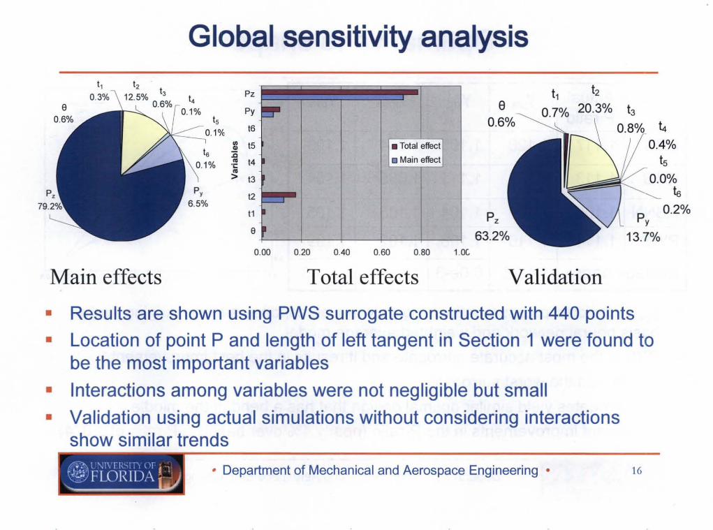
Global sensitivity analysis
t1 t20.7% 20.3% t3
0.8% 40.4%
ts0.0%
isP 0.2%
y
13.7%
Pz63.2%
12
11
e
I.pz
0.1% Py e16
0.6%
III IS • Talai effecl..:c
o Main effeci"' 14'1::
"'> 13
Main effects Total effects Validation
• Results are shown using PWS surrogate constructed with 440 points• Location of point P and length of left tangent in Section 1 were found to
be the most important variables
• Interactions among variables were not negligible but small• Validation using actual simulations without considering interactions
show similar trends
• Department of Mechanical and Aerospace Engineering • 16

Dimensionality reduction• Shape definition is same as used
earlier
• We fix six design variables nearto their optimal values asobserved for PRS design
• Fixed variables
• 8 = 60°
• t1 = 1.25
• t3 = 0.05
• t4 = 1.00
• t5 = 1.00
• t6 = 1.00
• Three design variables withexpanded range are -7
Section 1
Section 3
p (P" P,)
Min Max
~ 0.60 0.75
P -2.00 -1.50
Pz 5.85 6.00
• Department of Mechanical and Aerospace Engineering • 17

Optimization results• Optimization using sap when different surrogates approximate
response
• Optimized variables and responses
t2 Pv Pz Actual Y Yprs Ykrg Yrbnn Ypws
PRS 0.60 -1.99 6.00 1.150 1.151 1.151 1.155 1.152
KRG 0.60 -1.87 6.00 1.149 1.150 1.152 1.152 1.151
RBNN 0.61 -1.97 5.99 1.150 1.150 1.150 1.155 1.151
PWS 0.60 -1.96 6.00 1.150 1.151 1.152 1.154 1.152
Average absolute error 7.5e-4 1.5e-3 4.3e-3 1.7e-3
• All optimized designs are in the same region of design space andsignificantly better than the baseline design but a data point is better!
• The optimal design appeared at a corner that was already sampled
• PRS was the most accurate surrogate
• Department of Mechanical and Aerospace Engineering • 18

Flow fields
o·2Y
·4
RHO
560.00 RHO
8 52000 560.00490.00 8 520.00460.00 490.00430.00 460.0040000 430.00370.00 400.00
7 340.00 37000N 7 340.00
Baseline Optimal design
66
• Less separation and recirculation in the optimal design compared tothe baseline design
• High pressure rise near the exit for optimal design• More smooth turning of the flow
Optimal design reduce separation losses
• Department of Mechanical and Aerospace Engineering • 19

Vane loadings
-';--4~--'--';;--3~~~?""""--"'----'---';-1~-'---'--*'0 5.2
650
5.8
6N
5.6
6.2
Vane loadings
.....---.... Vane shapes 6.6~__ 6.4
=== Baseln. vaneIrtennediatll optimal
----- Optimal vane
== Baselne vaneIrtermedlatll optima!
----- Optimal vane400
450
550
600
• High pressure load near the inlet
• Pressure increases with decreasein area in the channel and viceversa
• Reduction in inlet tip load andpressure loading on the vane (areabound by the pressure profile) byoptimization
• Optimal vane shape experienceshighest mean pressure susceptible to failure because ofthe least material
• Department of Mechanical and Aerospace Engineering • 20

Summary
• Shape optimization of diffuser vane resulted in significantimprovements in pressure rise - nearly 7% improvement overbaseline design
• The optimal vane is thinner than baseline, allows smooth turningof the flow from both edges, and reduces separation but issusceptible to stress failure, and may not accommodatemanufacturing requirements
• Surrogate based optimization process helps• identify the most important design variables
• identify region of high performance and the near optimal design
• provide accurate predictions in the desired region
• Best surrogate model can change during optimization, henceusing multiple surrogates is advantageous
;.""1'\1\11\ 11 ' \lj .
~• Department of Mechanical and Aerospace Engineering • 21

Appendix
• Department of Mechanical and Aerospace Engineering •

Shape definition
Min Max
e 60 110
t1 1.25 2.50
t2 0.75 1.50
t3 0.05 0.30
t4 0.50 1.00
ts 0.50 1.00
ts 1.00 2.00
Py -2.50 -2.00
Pz 5.70 5.85
Sec:tion4
Sec:tion 1
Section 3
• ine design variables• define angle e• define lengths of tangent vectors t1-t6• coordinates of P: PY1 Pz
• Mesh generation using CORGRD - 13065 points• Each simulation takes nearly 20 minutes - use surrogates for optimization
• Department of Mechanical and Aerospace Engineering • 23

Global sensitivity analysis• Global sensitivity analysis (Sobol, 1993) is used to assess the
contribution of different variables to total variability - can identifythe importance of variables
Variance ..... V(f)=E((f-fof) Mean ..... / 0 =!!... !/(x)dxt dx2 ...dxNv
Variance V(f) = INvV I V ... v. H t t V V ??
d 't' .+ .. + + 1 N ow 0 ge ,', ,ii,' •.•.ecomposl Ion i=1 ' l5,i5,j5,Nv
Ij ... v J
Function 1 (x) = 10 + LJ;(xJ + LJ;j (xi,x j)+ ... + J;2... Nv (x"x2 , ••• ,xN,)
decomposition ~ !<j ,main effects intera~tions
such that 1fl...isdxk=O then v= .[ f2 dx.I n J i I
• Department of Mechanical and Aerospace Engineering • 24
Sensitivity index of main effect Sensitivity index of total effect

Design space refinement
• Two ways of design space refinement• add 330 more samples - total 440 points (Set B)
• use poor quality surrogates to identify the region where we mayhave improved performance (at least 0.5% improvement overbaseline) and add samples in that region -:- sampled 110 points(Set C)
• Simulations at these locations - one simulation for eachcase failed
• Fit surrogate models to individual data sets• reduced cubic polynomial response surface to the Set B data
• reduced quadratic polynomial response surface to the Set C data
~.~ ! \.1\ I I I:' \'1
~• Department of Mechanical and Aerospace Engineering • 25

Quality of surrogates in refined domains
Set B wPI SetC we
I
# of training points 439 109
Minimum of data 1.000 1.052
Mean of data 1.040 1.075
Maximum of data 1.097 1.105
PRS R2adj 0.959 0.978
PRESS 4.84e-3 0.50 8.74e-3 0.36
KRG PRESS 9.14e-3 0.27 9.47e-3 0.34
RBNN PRESS 1.17e-2 0.22 1.07e-2 0.30
PWS PRESS 6.07e-3 7.53e-3
• Surrogate predictions are improved - best surrogate changed• No lack of fit for both data sets• Potential of improvement using the surrogates fit to the Set C data
• Department of Mechanical and Aerospace Engineering • 26

•
Global sensitivity analysis
1.000.800.600.40
tara tion
Sensitivity index
0.20
t2
t1
ePy
5.2%
pz
14 Py0.3% t6
15 II> t5 • Total effect.,0.1% :c
• Main effect.. t4Is .1:..
0.6%> t3
ain effects 0.00
11
e 0.4%
0.4%
• Global sensitivity analysis using multiple surrogate models resulted insame conclusions - results shown are obtained using PWS
• Location of point P (Py' Pz) was most important followed by variable t2
• All other variables were relatively unimportant
• Interactions between different variables were not too important
Location of point P and parameter t are most important. .....
';.>-'1 ·\.1\[1, [I \lj
~• Department of Mechanical and Aerospace Engineering • 27

Validation of GSA results
Main effects - actual variance
• Vary one variable at a time while keepingall other variables fixed at mean values
• Calculate variance using trapezoidal rulewith five equi-spaced levels for eachvariable
• Actual sensitivity analysis also indicatethree important variables - t2 , Py' Pz
• The differences in results of GSA andactual computations are attributed to• insufficient data to cover entire design
space
• inaccuracies in surrogate models
• actual variance does not account for theinteractions
e0.6%
Pz
63.2%
t220.3% t3
0.8% t40.4%
t5
0.0%t6
P 0.2%y
13.7%
Results validate the lobal sensitivit anal sis. . - _.-
~• Department of Mechanical and Aerospace Engineering • 28

..
Performance of surrogates (Final)
• All data points were better P-ratio wthan the intermediate
# of trainingoptimal design 20
points
• Reduced quadratic fit of Minimum of data 1.117
pressure ratio in modified Mean of data 1.136
design space Maximum of data 1.151
• No lack of fit Baseline design 1.074
• Quality of PRS is the best PRS R2adj 0.956
and RBN N is the worst PRESS 2.74e-3 0.59
• PWS is at par with the KRG PRESS 7.14e-3 0.25
best surrogate RBNN PRESS 1.11 e-2 0.16
PWS PRESS 4.21e-3
• Department of Mechanical and Aerospace Engineering • 29