improving the knowledge-based expert system lifecycle
TRANSCRIPT

UNF Digital Commons
UNF Graduate Theses and Dissertations Student Scholarship
2012
Improving the Knowledge-Based Expert SystemLifecycleLucien MilletteUniversity of North Florida
This Master's Thesis is brought to you for free and open access by theStudent Scholarship at UNF Digital Commons. It has been accepted forinclusion in UNF Graduate Theses and Dissertations by an authorizedadministrator of UNF Digital Commons. For more information, pleasecontact Digital Projects.© 2012 All Rights Reserved
Suggested CitationMillette, Lucien, "Improving the Knowledge-Based Expert System Lifecycle" (2012). UNF Graduate Theses and Dissertations. 407.https://digitalcommons.unf.edu/etd/407

IMPROVING THE KNOWLEDGE-BASED EXPERT SYSTEM LIFECYCLE
by
Lucien Millette
A thesis submitted to the School of Computing
in partial fulfillment of the requirements for the degree of
Master of Science in Computer and Information Sciences
UNIVERSITY OF NORTH FLORIDA SCHOOL OF COMPUTING
March, 2012

ii
Copyright (©) 2012 by Lucien Millette
All rights reserved. Reproduction in whole or in part in any form requires the prior written permission of Lucien Millette or designated representative.

Signature Deleted
Signature Deleted
Signature Deleted
Signature Deleted
Signature Deleted
Signature Deleted

iv
ACKNOWLEDGEMENT
I would like to thank Dr. Behrooz Seyed-Abbassi for his guidance and support
throughout this entire process. I would also like to send a special thanks to my
girlfriend, Leann, for her editorial guidance. Finally, I would like to thank my parents,
Jim and Mary, for being great role models and teaching me to never give up.

v
CONTENTS
List of Figures ................................................................................................................. vii
Abstract ............................................................................................................................. ix
Chapter 1: Introduction .................................................................................................... 1
1.1 Knowledge-Based Expert System Components .................................................. 1
1.2 Barriers to Knowledge Acquisition ..................................................................... 3
1.3 Issues Associated with Knowledge Base Maintenance ....................................... 5
1.4 Opportunities for Improvement ........................................................................... 7
1.5 Organization ........................................................................................................ 7
Chapter 2: Overview of Knowledge-Based Expert Systems ........................................... 8
2.1 Knowledge-Based Expert System Lifecycle ....................................................... 8
2.2 Artificial Intelligence ......................................................................................... 14
2.3 Data Warehousing ............................................................................................. 19
2.4 Extraction Transformation Loading (ETL) Tools and Data Mining ................. 22
Chapter 3: Methodology ................................................................................................. 26
3.1 Enhanced Knowledge Acquisition .................................................................... 28
3.2 Integration of Artificial Intelligence for Knowledge Base Maintenance .......... 29
3.3 Advantages of the Improved Methodology ......................................................... 31
Chapter 4: Implementation ............................................................................................. 33
4.1 Phase 1 – Assemblage of Relevant Facts and Rules .......................................... 33
4.2 Phase 2 – Knowledge Acquisition for the Knowledge Base Data Warehouse .. 35
4.3 Phase 2.1 – Data Mining for the Knowledge Base Data Warehouse ................ 36

vi
4.4 Phase 3 – Data Modeling for the Knowledge Base Data Warehouse ................ 37
4.5 Phases 4 and 4.1 – Knowledge Representation and Historical Data
Transformation .......................................................................................................... 38
4.6 Phase 5 – Inference Engine Creation ................................................................. 40
4.7 Phase 5.1 – Artificial Intelligence Implementation ........................................... 42
4.8 Phase 6 – User Interface Design ........................................................................ 44
4.9 Phase 7 – Testing ............................................................................................... 45
4.10 Knowledge-Based Expert System Software .................................................... 46
Chapter 5: Results Analysis ........................................................................................... 52
5.1 Artificial Intelligence Control Experiment ........................................................ 52
5.2 Inference Engine Minimum Percentage Experiment ......................................... 56
5.3 Final Comparison ............................................................................................... 62
Chapter 6: Conclusions and Future Work ..................................................................... 66
6.1 Conclusions ........................................................................................................ 66
6.2 Future Work ....................................................................................................... 69
References ........................................................................................................................ 70
Appendix A: Example of User Interface Source Code .................................................. 75
A.1 ViewSolutions.aspx .......................................................................................... 75
A.2 ViewSolutions.aspx.vb ..................................................................................... 76
Appendix B: Example of Business Layer Source Code ................................................ 79
Appendix C: Example of Data Access Layer Source Code .......................................... 83
Appendix D: Example of Stored Procedures ................................................................. 86
Appendix E: Database and Data Warehouse SQL ........................................................ 88
Vita .................................................................................................................................. 93

vii
List of Figures
Figure 1: Knowledge-Based Expert System Components ................................................. 3
Figure 2: Knowledge-Based Expert System Lifecycle ...................................................... 9
Figure 3: Traditional Knapsack Problem Definition ....................................................... 15
Figure 4: Container-Loading Algorithm .......................................................................... 17
Figure 5: Orthogonality Test ........................................................................................... 19
Figure 6: Example of Star Schema .................................................................................. 20
Figure 7: Example of Snowflake Schema ....................................................................... 22
Figure 8: Methodology Comparison ................................................................................ 26
Figure 9: Proposed Knowledge-Based Expert System Lifecycle .................................... 27
Figure 10: Proposed Knowledge-Based Expert System Components ............................. 32
Figure 11: Example of Transportation System Data Set ................................................. 36
Figure 12: Data Warehouse Schema ................................................................................ 38
Figure 13: Associate Rule Learning Process ................................................................... 39
Figure 14: Inference Engine Process ............................................................................... 41
Figure 15: Artificial Intelligence Algorithm .................................................................... 44
Figure 16: Login Screen .................................................................................................. 46
Figure 17: Main Screen ................................................................................................... 47
Figure 18: Problem Details Page ..................................................................................... 48
Figure 19: View Solution Page ........................................................................................ 49
Figure 20: Adding Potential Rules from the Artificial Intelligence ................................ 50
Figure 21: Results Analysis Page .................................................................................... 51
Figure 22: Artificial Intelligence Control Experiment Results ........................................ 54

viii
Figure 23: Artificial Intelligence Control Experiment Results Chart .............................. 54
Figure 24: Artificial Intelligence Control Experiment Percentage Full Statistics ........... 55
Figure 25: Artificial Intelligence Control Experiment Percentage Graph ....................... 56
Figure 26: Container Counts for Minimum Percentage Experiment ............................... 57
Figure 27: Percentages of the Absolute Minimum Values .............................................. 58
Figure 28: Graphical Percentages of the Absolute Minimum Values ............................. 59
Figure 29: Graph of Average Percentages of the Absolute Minimum ............................ 59
Figure 30: Average Percentage Full of Containers .......................................................... 61
Figure 31: Graph of Percentage Full of Containers ......................................................... 61
Figure 32: Averages of Percentage Full of Containers .................................................... 62
Figure 33: Final Comparison Statistics ............................................................................ 63
Figure 34: Final Comparison Graph ................................................................................ 63
Figure 35: Average Percentage Full Final Statistics ........................................................ 65
Figure 36: Average Percentage Full Final Graph ............................................................ 65

ix
ABSTRACT
Knowledge-based expert systems are used to enhance and automate manual processes
through the use of a knowledge base and modern computing power. The traditional
methodology for creating knowledge-based expert systems has many commonly
encountered issues that can prevent successful implementations. Complications during
the knowledge acquisition phase can prevent a knowledge-based expert system from
functioning properly. Furthermore, the time and resources required to maintain a
knowledge-based expert system once implemented can become problematic.
There are several concepts that can be integrated into a proposed methodology to
improve the knowledge-based expert system lifecycle to create a more efficient process.
These methods are commonly used in other disciplines but have not traditionally been
incorporated into the knowledge-based expert system lifecycle. A container-loading
knowledge-based expert system was created to test the concepts in the proposed
methodology. The results from the container-loading knowledge-based expert system
test were compared against the historical records of thirteen container ships loaded
between 2008 and 2011.

-1-
Chapter 1
INTRODUCTION
Starting in the late 1950’s and early 1960’s, computer programs were written with the
explicit goal of problem solving [Giarratano89]. Knowledge-based expert systems are
one manifestation of the applications that trace their roots back to those early programs.
Knowledge-based expert systems are computer systems that have expertise in a given
domain and are useful when analyzing and processing large amounts of data in a short
amount of time [Grosan11] [Dabbaghchi97]. They use knowledge that has been gathered
and stored within the knowledge base in order to solve problems in the specific domain
for which they were created.
Organizations are always at risk of losing experts in key areas within their business
processes due to turnover, illness, or death. Knowledge-based expert systems help
alleviate such risks by taking the knowledge obtained by experts, also called problem
domain experts, over the course of their careers and storing it within a knowledge base.
A knowledge-based expert system can also reduce the amount of time problem domain
experts will require to solve problems in the problem domain. A problem domain is a
specific area of business process for which a knowledge-based expert system is created to
support.
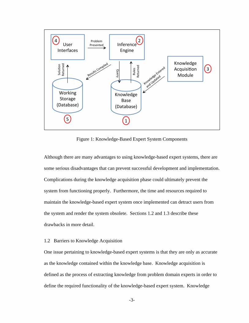
1.1 Knowledge-Based Expert System Components
Knowledge-based expert systems are composed of several independent components.
Figure 1, as described by Grosan and Hoplin [Grosan11] [Hoplin90], shows the

-2-
independent components and how they work together to solve a problem within the
problem domain. The arrows depicted in Figure 1 outline the flow of information
throughout the system. The first component is the knowledge base in which heuristic
knowledge of the domain experts as well as pertinent facts about the problem are stored
[Grosan11] [Hoplin90]. The second component is the inference engine that utilizes
strategies from the searching and sorting domains to test the rules contained in the
knowledge base on a particular problem. The inference engine accomplishes this by
querying information from the knowledge base and applying the returned results. The
knowledge acquisition module, the third component, facilitates the transfer of knowledge
into the knowledge base for future use [Grosan11] [Hoplin90]. The fourth component is
the user interface that allows users to interact with the knowledge-based expert system by
presenting the problem to the inference engine and viewing solutions. The fifth
component is the working storage which the knowledge-based expert system uses to store
information while a specific problem is being solved [Aniba09] and then contains the
information pertaining to the solution.
-3-
Figure 1: Knowledge-Based Expert System Components
Although there are many advantages to using knowledge-based expert systems, there are
some serious disadvantages that can prevent successful development and implementation.
Complications during the knowledge acquisition phase could ultimately prevent the
system from functioning properly. Furthermore, the time and resources required to
maintain the knowledge-based expert system once implemented can detract users from
the system and render the system obsolete. Sections 1.2 and 1.3 describe these
drawbacks in more detail.
1.2 Barriers to Knowledge Acquisition
One issue pertaining to knowledge-based expert systems is that they are only as accurate
as the knowledge contained within the knowledge base. Knowledge acquisition is
defined as the process of extracting knowledge from problem domain experts in order to
define the required functionality of the knowledge-based expert system. Knowledge
!"#$%&'(&)*+,&)
-.+/+0+,&1)
2"3&4&"5&)6"(7"&)
8,&4)2"/&43+5&,)
9#4:7"();/#4+(&)
-.+/+0+,&1)
!"#$%&'(&)<5=>7,7?#")@#'>%&)
!"#$
%&'(&)
6"/&4
&'))
+"')8A
'+/&'
)
B>&4C)
D>%&,))
D&/>
4"&'
)
D&,>%/,
)E#FA7%&
');#
%>?#
"))
D&/>
4"&'
)
G4#0%&F)G4&,&"/&')
H)
I)
J)
K)
L)

-4-
acquisition has been referred to as the “bottleneck in the process of building expert
systems” [Golabchi08] [Forsythe89]. The two key groups of stakeholders during
knowledge acquisition are the knowledge engineer and the problem domain experts. The
knowledge engineer acts as the conduit for extracting domain specific information from
the problem domain experts.
The capability of the system is limited by the intelligence and quality of the interviews
conducted between the knowledge engineer and the problem domain experts
[Mertens04]. Research has been conducted to create standardized frameworks for the
knowledge acquisition process. However, the process still relies exclusively on the
manual transfer of knowledge from the problem domain experts to the knowledge
engineer, thus the success of the process lies entirely on the interviewing capabilities of
the knowledge engineer [Wagner86].
Lack of communication is a common problem encountered during the knowledge
acquisition phase. There are a multitude of causes starting with issues of missing
common terminology and misconceptions made by both the knowledge engineer and the
problem domain experts [Hardaway90]. During the interview process the knowledge
engineer attaches to a problem domain expert or a group of problem domain experts for a
significant amount of time. Personality issues can arise between knowledge engineers
and problem domain experts and can create a serious barrier to the knowledge acquisition
process [Golabchi08] [Forsyhte89]. Also not all problem domain experts are familiar
with information technologies and thus can be reluctant to participate in the development
effort. They often do not believe that any automated system can be created to support
their complex business processes. Additionally, if the problem domain experts feel that

-5-
the knowledge-based expert system can undermine their knowledge and make their jobs
seem obsolete, they will be unlikely to assist the knowledge engineer in the development
effort.
The knowledge acquisition processes developed were traditionally centered on gathering
information directly from the problem domain experts. There were no existing
searchable databases containing historical records of problem domain expert’s work.
Modern experts no longer predominantly use pencil and paper to solve problems.
Instead, they use some form of software application created to help them work through
the problem and create a solution. The process is still manual because all knowledge still
resides with the experts. However, the solutions created using the software based on the
manual methods are stored and archived using modern techniques. The modern archival
techniques create a searchable historical database or data warehouse of problems and
solutions created by experts in the problem domain. The databases can be as simple as
spreadsheets stored on a hard drive or can be full-scale database management systems.
Traditional knowledge-based expert system implementations do not utilize the
information contained in these historical data repositories even though these repositories
contain valuable information that could be mined into the knowledge base for future use.
1.3 Issues Associated with Knowledge Base Maintenance
Another issue with knowledge-based expert systems arises in the fact that the domains
that these systems are created to function in are dynamic in nature. In order for the
system to remain relevant, it must adapt to the changing conditions within the problem
domain. Knowledge-based expert systems cannot adapt on their own or create new
innovative ways of solving problems [Grosan11] [Hoplin90]. The way that the

-6-
knowledge-based expert systems adapt is through maintenance of the knowledge
contained within the knowledge base. The difficulty associated with maintaining a
knowledge base is dependent on how complex the data structure of the knowledge base is
and how well the knowledge acquisition module is constructed. Not all problem domain
experts are information technology experts, and therefore knowledge base maintenance
can be difficult and time consuming. The knowledge engineer must work with the
problem domain experts as soon as a new variable is introduced into the problem domain
to ensure the knowledge is updated into the knowledge base properly. This implies that
knowledge base maintenance is an ongoing process that can require significant
investments of time from both knowledge engineers and problem domain experts after
the system has been implemented.
The amount of time necessary to keep up with knowledge base maintenance can present
significant problems to an organization. The experts in the problem domain can be
extremely busy, can retire, or leave the company for a host of different reasons.
Furthermore, information technology personnel are typically stretched thin. They often
do not have the necessary resources to train a knowledge engineer to work with the
problem domain experts as often as is required to keep up with the maintenance. Thus,
problem domain experts are typically left to maintain the knowledge base on their own.
This can be frustrating to the problem domain experts and can create a lack of trust in the
system as a whole. Problem domain experts would be more apt to revert to the manual
method of solving problems as opposed to maintaining the knowledge base.

-7-
1.4 Opportunities for Improvement
In order for a knowledge-based expert system to be successfully implemented, the issues
discussed above must be mitigated. This thesis will incorporate several tools and
techniques not typically associated with knowledge-based expert system development
into an improved methodology designed specifically to mitigate the risks described
above. The first improvement to the traditional methodology is to enhance the
knowledge acquisition phase. Data mining and data warehousing techniques can be
utilized to enhance and streamline the knowledge acquisition phase. The second
improvement is to change the way knowledge base expert systems are maintained post
implementation. By utilizing the power of artificial intelligence to aid problem domain
experts, the resources and time required to keep the knowledge base maintained can be
drastically reduced.
1.5 Organization
The second chapter of this thesis will provide an overview of the knowledge-based expert
system lifecycle. The second chapter will also provide background information on the
tools and techniques that will be incorporated into the improved knowledge-based expert
system methodology. The third chapter will describe the improved methodology in
detail. The fourth chapter will describe an implementation of a knowledge-based expert
system using the improved methodology in the container-loading domain. The fifth
chapter will present the results from implementing the knowledge-based expert system.
The sixth chapter will present the conclusions of this thesis and opportunities for future
research.

-8-
Chapter 2
OVERVIEW OF KNOWLEDGE-BASED EXPERT SYSTEMS
This chapter provides an overview of the background concepts that support the improved
knowledge-based expert system methodology. Section 2.1 describes the traditional
knowledge-based expert system lifecycle. Section 2.2 summarizes basic concepts in
artificial intelligence and provides specific examples that will be incorporated in the
proposed container-loading knowledge-based expert system implementation. Section 2.3
describes the basic concepts associated with data warehousing that will be incorporated in
the improved knowledge-based expert system methodology. Section 2.4 outlines extract
transformation load (ETL) processes and data mining techniques that can be used to help
enhance the knowledge acquisition phase in the improved knowledge-based expert
system methodology.
2.1 Knowledge-Based Expert System Lifecycle
The creation of a knowledge-based expert system requires that an appropriate problem
statement be constructed. There must be a problem that justifies the amount of effort and
cost necessary to implement knowledge-based expert systems for all stakeholders. As
with all software implementations, a formal process must be followed to ensure
requirements from all levels of an organization are met. Software development
methodologies are continually evolving and thus affect how knowledge-based expert
systems are developed [Golabchi08]. Modern knowledge-based expert systems are
-9-
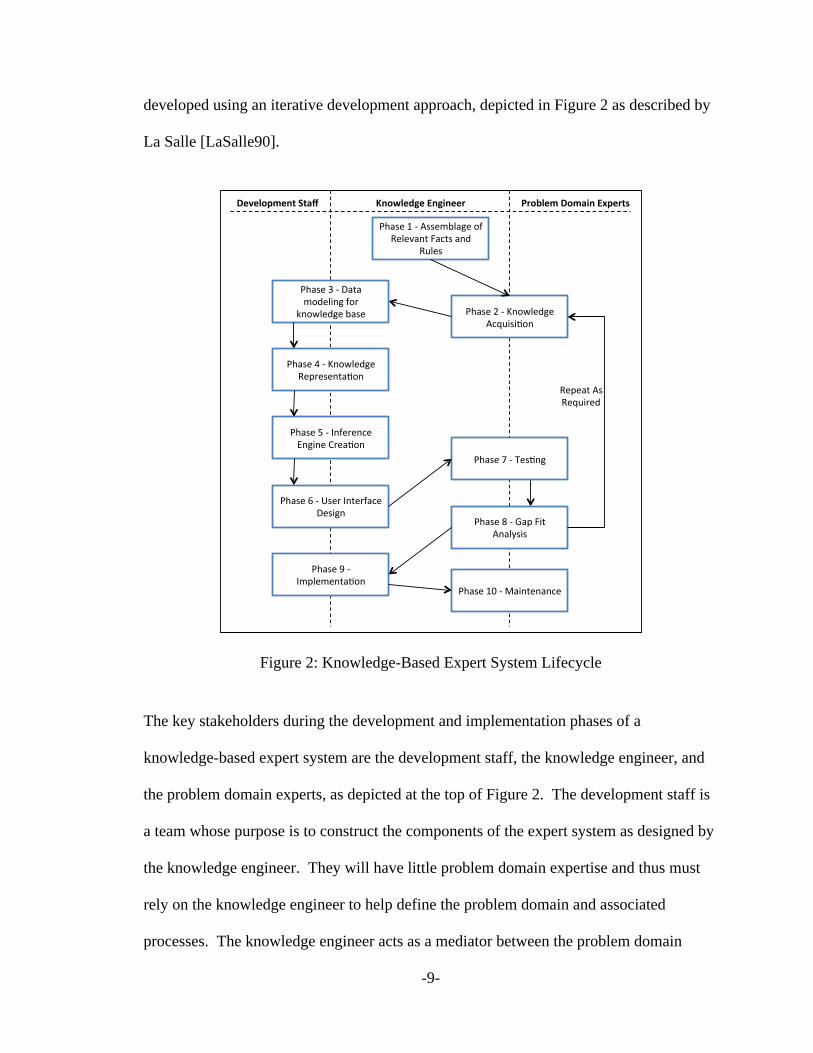
developed using an iterative development approach, depicted in Figure 2 as described by
La Salle [LaSalle90].
Figure 2: Knowledge-Based Expert System Lifecycle
The key stakeholders during the development and implementation phases of a
knowledge-based expert system are the development staff, the knowledge engineer, and
the problem domain experts, as depicted at the top of Figure 2. The development staff is
a team whose purpose is to construct the components of the expert system as designed by
the knowledge engineer. They will have little problem domain expertise and thus must
rely on the knowledge engineer to help define the problem domain and associated
processes. The knowledge engineer acts as a mediator between the problem domain
!"#$%&'(&)*"(+"&&,)-&.&%#/0&"1)2134) 5,#6%&0)-#03+")*7/&,18)
!"#$%&'&(&)$$%*+,#-%&./&0%,%1#23&4#53$&
07,%$&
!"#$%&8&(&92.:,%6-%&)5;7<$<=.2&
!"#$%&>&(&?#3#&*.6%,<2-&/.@&
A2.:,%6-%&+#$%&
!"#$%&B&(&92.:,%6-%&0%C@%$%23#=.2&
!"#$%&D&(&E2/%@%25%&F2-<2%&G@%#=.2&
!"#$%&H&(&I$%@&E23%@/#5%&?%$<-2&
!"#$%&J&(&K#C&4<3&)2#,L$<$&
!"#$%&M&(&N%$=2-&
0%C%#3&)$&&0%;7<@%6&
!"#$%&O&(&E*C,%*%23#=.2&
!"#$%&'P&(&Q#<23%2#25%&

-10-
experts and the development staff. The knowledge engineer must understand both the
technical capabilities of the development staff and also be able to draw out expertise from
the problem domain experts. The knowledge engineer must gather system requirements
and draw problem domain specific knowledge out of the experts in order for the
knowledge base to be filled. In addition to being the end users of the knowledge-based
expert system, the problem domain experts understand the requirements and knowledge
necessary to construct a knowledge-based expert system.
The first step in the software development lifecycle is for the knowledge engineer to
become acclimated with the problem domain, as shown as Phase 1 of Figure 2. The
knowledge engineer is then responsible for gathering and interpreting knowledge
acquired from problem domain experts into the knowledge base [Grosan11] [Hoplin90].
The knowledge engineer must start gathering information and understanding domain
specific terminology prior to conducting any formal meetings or interviews with the
problem domain experts. Becoming more acclimated with the domain specific
terminology enables the knowledge engineer to communicate with the problem domain
experts, and thus aids the knowledge engineer with understanding problem solving in the
problem domain.
Knowledge acquisition, Phase 2 of Figure 2, is the process of extracting knowledge from
problem domain experts by the knowledge engineer [Grosan11] [Hoplin90]. The goals
during the knowledge acquisition phase are to gather system requirements and to
document knowledge needed to construct the knowledge base. The knowledge engineer
must gather the complete breadth and depth of knowledge from the problem domain
experts that will be required to completely solve problems in the problem domain. The

-11-
completeness and correctness of the knowledge base is a critical factor to a knowledge-
based expert system’s success. The knowledge engineer must determine all steps used by
problem domain experts in order to solve problems and then turn such steps into detailed
requirements for the development staff. Traditionally the knowledge engineer performs a
series of interviews with the problem domain experts during the knowledge acquisition
phase. The interviews can be conducted using various techniques to facilitate the
knowledge transfer from the problem domain experts to the knowledge engineer.
The next phase in development is data modeling for the knowledge base, as shown in
Phase 3 of Figure 2. Using the information collected during the knowledge acquisition
phase, knowledge engineers use modern data modeling techniques, such as logical and
physical modeling, to construct the data structure needed to house the information
permanently. As knowledge-based expert systems have evolved, databases have become
the standard method of storing and maintaining knowledge in knowledge bases
[Grosan11] [Hoplin90].
Once the knowledge acquisition and knowledge base data modeling phases have
completed, the knowledge engineer then can begin the knowledge representation phase,
as shown in Phase 4 of Figure 2. The knowledge representation phase is defined as the
process of translating data into a form useable by a computer system [Hoplin90]. In this
phase, the knowledge extracted from the problem domain experts, during the knowledge
acquisition phase, is translated into the data structure of the knowledge base. The goal of
this phase is to create the data necessary for the initial implementation of the knowledge
base.

-12-
Knowledge-based expert system methodology is best implemented as an iterative
process. Knowledge engineers do not traditionally have experience or training in the
processes that make the knowledge acquisition phase successful [La Salle90]. Therefore,
the knowledge acquisition, data modeling, and knowledge representation phases can be
performed iteratively until the knowledge base represents the complete breadth and depth
of knowledge in the problem domain. Iterating through the knowledge acquisition, data
modeling, and knowledge representation phases allows for the knowledge engineer to
work out the complexities of the problem domain gradually and test the expanding data
model [Grosan11] [La Salle90].
The next phase in development is the creation of the inference engine, as depicted in
Phase 5 of Figure 2. The main function of the inference engine is to take a problem and
search the knowledge base for rules to apply in order to produce a solution. The
inference engine should function following the requirements gathered by the knowledge
engineer from the problem domain experts. Completeness, correctness, and speed are the
three main concepts that must be achieved in an optimal inference engine [Grosan11]
[Hanson90]. The inference engine must also be able to traverse all possible combinations
of rules in order to design an optimal solution. All solutions created must be correct and
reached in a reasonable amount of time. The two types of inference engine
implementations are forward chaining and backward chaining [Mattos03]. The problem
domain will dictate which implementation the knowledge engineer and development staff
select to build for an inference engine.
After the inference engine is created, the next phase of the knowledge-based expert
system lifecycle is the creation of the user interfaces, as shown in Phase 6 of Figure 2.

-13-
User interfaces allow users to present a problem to the system, view solutions created by
the system, and perform maintenance on the knowledge base [La Salle90]. The user
interface can be implemented in a variety of ways, including web pages, application
forms, or any other modern techniques.
Once the user interfaces are constructed, the system is ready to be tested, as shown in
Phase 7 of Figure 2. The most common testing technique is a comparison to a manually
solved problem by the problem domain experts. If the solutions vary, the knowledge
engineer would have to conduct a gap fit analysis, as shown in Phase 8 of Figure 2. The
gap fit analysis would then highlight where the discrepancy originated and the knowledge
engineer would either modify the knowledge base or the inference engine algorithms.
The testing and gap fit analysis phases are additional iterative processes that allow the
knowledge engineer and development staff to gradually evolve towards the final product.
Multiple problems spanning the entire problem domain must be analyzed to ensure the
knowledge-based expert system’s conclusions are compatible with those of the problem
domain experts.
Once the knowledge-based expert system can correctly solve problems previously solved
by the problem domain experts, the knowledge-based expert system can be used to solve
new problems. Initial implementations, Phase 9 of Figure 2, often resemble the testing
phase in that the problem domain experts will solve the problem simultaneously to ensure
the system is functioning properly. However, after initial implementation success, the
knowledge-based expert system is ready to function independently.

-14-
After the initial implementation of the knowledge-based expert system, the lifecycle is
not complete. Maintenance is required after implementation for knowledge-based expert
systems, as shown in Phase 10 of Figure 2. The problem domains for which knowledge-
based expert systems are developed are never static. As the problem domains evolve,
knowledge-based expert systems must also evolve. The knowledge acquisition module
becomes paramount to maintain the system’s effectiveness. The problem domain experts
must constantly analyze new conditions introduced to the problem domain and adjust the
knowledge base accordingly. If the knowledge base is left stagnant and changes to the
environment are not incorporated, then the knowledge-based expert system will become
outdated, ineffective, and possibly incorrect.
2.2 Artificial Intelligence
The first new concept that will be incorporated into the improved methodology is
artificial intelligence. Artificial intelligence is a broad field with the goal of making
computers capable of solving problems in a particular domain [Millinton09]. Artificial
intelligence theory extends into the realm of human thought and how humans process
thoughts to reach conclusions. The term artificial intelligence was coined in 1956 with
the earliest work in the field dating back to the end of World War II [Russell03]. The
impact of research in artificial intelligence can be seen in everything from Bayesian
filters for email, commonly called spam filters, to computer games with realistic
algorithms to model game play and everything in between.
One specific area of research is known as the knapsack problem. The classic knapsack or
rucksack problem, as shown in Figure 3, is defined as follows: given n items, with each

-15-
item j having an integer profit pj and an integer weight wj, choose a subset of items such
that their overall profit is maximized without exceeding a total weight c [Pisinger05].
Figure 3: Traditional Knapsack Problem Definition
The traditional knapsack problem and the derived problems based off of the knapsack
problem are defined as NP-hard [Khan02] [Russell03]. A problem being designated NP-
hard means that an algorithm cannot be created to construct the most optimal solution to
the problem in polynomial time. However, researchers have been able to create
algorithms that create an approximately optimal solution for NP-hard problems within
polynomial time.
The shipping industry has invested heavily in research in solving the knapsack problem
[Whelan96]. Algorithms based off the knapsack problem have been developed to support
many processes central to the business of shipping. I.D. Wilson’s algorithm is one
example of how research is being done into the optimization of how containers are
stowed aboard a container ship [Wilson99]. Container ships travel in circular routes
across the globe with multiple ports of embarkation and debarkation. The goal of
Wilson’s algorithm is to minimize the number of container lifts needed to unload the
containers at each port. Wilson’s algorithm takes into account the different types of lifts

-16-
that would be required to access each container and identifies which port each container
needs to be unloaded. When containers block access to other containers that must be
unloaded at a particular port, they have to be lifted and temporarily moved. Each lift
costs the shipping company money so reducing the number of lifts at each port is in the
best financial interest for shipping companies. Wilson’s algorithm can create a load plan
that minimizes the cost for a shipping company.
Another area of research related to the knapsack problem in the shipping industry is the
automation of the container packing process. Customers order varying numbers of
products that must be packed by shipping companies and shipped via standard sized
shipping containers. Loading different numbers of products of varying sizes is an area of
interest for research in artificial intelligence. Kun He and Wenqi Huang have developed
an algorithm to support this process in which a single container with objects of varying
sizes is loaded [He10] [Huang07].
He and Huang’s algorithm utilizes a caving degree calculation as a metric to determine
the best item to load next in the loading process and has shown promising results in
reliability and speed. The algorithm, as shown in Figure 4, maintains the available
corners within the container in which items may be loaded. Each item that still needs to
be loaded is provisionally loaded by the algorithm into each available corner and the
caving degree is then calculated. After all items have been provisionally loaded into each
corner available, the one that produced the highest caving degree is loaded. The
algorithm then updates the list of available corners after loading that particular item. The
process then repeats itself until the container is loaded or there are no more items to be
loaded.

-17-
Figure 4: Container-Loading Algorithm
There are three factors taken into account when calculating the caving degree. The first
factor is how much surface area of the item being loaded is flat against another surface
within the container. The second factor is how far the item is from the other surrounding
objects. The final factor is the total volume of the item. He and Huang’s algorithm
produces an approximation of the best way to load a container, by utilizing the caving
degree calculation, without having to test all possible ways of loading a container. This
allows the algorithm to function in a reasonable amount of time. He and Huang’s
algorithm creates an approximate solution to a NP-hard problem with a high degree of
reliability.
Each time an item is loaded in He and Huang’s algorithm, the collection is updated with
new available corners and corners that are now blocked are removed. In order to
accomplish the update to the collection of corners, concepts from multivariable calculus
Create list of available items Create collection of available corners and insert the origin While there are still available items that can fit in the container {
For each available corner { For each type of available item { For each valid item orientation { Provisionally pack the item into the corner with the current orientation If the item fits in the corner given container size and other objects already
packed { Compute Caving Degree } } } Pack the item with the highest Caving Degree calculation Update the list of available corners Update the list of available items }
}

-18-
have to be introduced. A corner, according to He and Huang, is defined as an unoccupied
point in three-dimensional space where three orthogonal surfaces meet [Huang07]
[He10]. Two surfaces, or planes, are called orthogonal if the normal vectors of those
surfaces are perpendicular [Stewart05]. Therefore in order for a point, or coordinate, in
three-dimensional space to meet the criteria for an available corner according to He and
Huang, each surface that contains the coordinate must be evaluated. When an item is
loaded, the corner in which the object was loaded into is removed from the collection.
The seven other corners of the object being loaded must be evaluated to see if they meet
the criteria of an available corner. Furthermore, any existing corners that intersect with
the object must be reevaluated to see if they still meet the criteria for an available corner.
The process for evaluating a potential corner, as described in Figure 5, begins by finding
all objects that intersect that corner, to include the container walls and floor. Then for
each object that intersects the potential corner, the specific plane or planes that intersect
the potential corner must be identified. Once each plane is identified, two vectors on
each plane must be constructed. By taking the cross product of the two vectors, a normal
vector is constructed for each plane. The normal vectors of all the planes that intersect
with the potential corner are then tested by calculating the dot product of each
combination of normal vectors. If the dot product of the normal vectors of three planes
all equal zero simultaneously then the corner meets the criteria identified by He and
Huang.

-19-
Figure 5: Orthogonality Test
2.3 Data Warehousing
The second new concept that will be incorporated into the improved methodology is data
warehousing. “A data warehouse is a large repository of historical data that can be
integrated for decision support” [Teorey11] [Teorey06]. Many organizations today have
vast amounts of data yet little information is drawn out of all that data. “Data
warehousing is a process, not a product, for assembling and managing data from various
sources for the purpose of gaining a single detailed view of part or all of a business”
[Gardner98]. Data warehouses leverage the historical data from a company and turn it
into useful information to support decision making. The goal of constructing a data
Known Info: Three points each plane: P0 = (x0,y0,z0) P1=(x1,y1,z1) P2=(x2,y2,z2) Step 1: Construct 2 Vectors on the Plane for each Plane P0P1 = (x1-x0,y1-y0,z1-z0) = <a> = (xa,ya,za) P0P2 = (x2-x0,y2-y0,z2-z0) = <b> = (xb,yb,zb) Step 2: Construct Cross Product to Create Normal Vector for each Plane <a> X <b> = <yazb-ybza, zayb-xazb, xayb-yaxB> Step 3: Test Dot product of all three normal Vectors to see if they equal 0 Normal Vector for plane 1 = <n1> = <n1x,n1y,n1z> Normal Vector for plane 2 = <n2> = <n2x, n2y, n2z> Normal Vector for plane 3 = <n3> = <n3x, n3y, n3z> Ensure that: <n1> · <n2> = n1x*n2x + n1y*n2y + n1z*n2z = 0 <n1> · <n3> = n1x*n3x + n1y*n3y + n1z*n3z = 0 <n2> · <n3> = n2x*n3x + n2y*n3y + n2z*n3z = 0

-20-
warehouse is to provide fast access to historical data that has been archived in such a
manner as to provide useful information for decision making while minimizing the size
of transactional databases [Kimball94].
Designing a data warehouse requires a different methodology than is required for
traditional transactional databases. Data warehouses are created by using one of two
basic structures: the star schema or the snowflake schema. A star schema has one main
fact table that is connected to many smaller supporting tables known as dimension tables,
as shown in Figure 6 [Teorey06]. Fact tables store the attributes and measures associated
with information in the data warehouse. A dimension table stores the additional
referential attributes, known as dimensions, for data stored within a fact table [Teorey11]
[Teorey06]. Dimension tables are also where hierarchical data is stored that can be used
for analysis.
Figure 6: Example of Star Schema

-21-
If the supporting dimension tables are normalized to show a hierarchy in the data, as
shown in Figure 7, then the schema is known as a snowflake schema. In general,
normalizing the dimension tables will slow down processing time, but can be critical in
creating a logical separation of data [Levene03]. The goal of data warehousing is to
provide historical data for decision support, so the types of data that need to be extracted
from the data warehouse will dictate whether a star schema or snowflake schema is used.
Once the schema has been created for the data warehouse, data from one or more
operational transactional based databases are processed into a data warehouses in batches
at some predefined interval [Levene03]. Data warehouses grow without bounds; this
unregulated growth is a deviation from traditional operational databases. Traditional
operational databases are kept relatively small with old data being purged periodically.
As the data is processed into a data warehouse it is typically translated into an order of
larger magnitude, meaning specific details are aggregated in order to support long term
trend analysis [Levene03].

-22-
2.4 Extraction Transformation Loading (ETL) Tools and Data Mining
The final concepts that will be incorporated into the improved methodology are
extraction transformation loading (ETL) tools and data mining. ETL tools are software
components that have the capability to extract data from one or multiple data sources,
transform or customize that data, and then insert the transformed data into a data
warehouse [Vassiliadis02]. ETL tools are sold commercially or can be created by an
organization for their data warehouse.
The extraction phase of the ETL process is where the raw data is pulled out of the various
data sources. In order for the extraction process to occur, there must be a temporary
storage location with a data model that can support data from the various data sources.
Figure 7: Example of Snowflake Schema

-23-
The temporary data storage must be capable of holding data that needs to be transformed
into the data model of the data warehouse it is destined for [Skautas11].
The transformation phase of the ETL process begins as the data is extracted out of the
temporary storage location and then cleansed and transformed into the data that will be
inserted into the data warehouse. The transformation techniques used in this phase are
common with data mining. “Data mining is the automatic extraction of implicit and
interesting patterns from large data collections” [Romero07]. The process of data mining
allows for new patterns to be identified in data. Data mining has been used to discover
new patterns and trends in many industries and fields to include medical drug testing,
educational trends, and sports analysis. Data mining can be customized as needed to
support a variety of data, but there are four basic concepts that are at the center of all data
mining applications supporting ETL processes: classification, regression, clustering, and
association rule learning.
Classification, also known as supervised learning, is a data mining technique, used during
the transformation phase of ETL, in which data is mapped into one of several predefined
groups based off of specific criteria [Fayyad96]. The first step in classification is to setup
the model for which data will be classified into by defining the different data sets that
need to be identified. The second step is to parse the data set and identify which data
belongs in which data set [Lutu02]. Classification is used to study financial market
trends, credit scoring, geospatial analysis, and many other domains.
Regression is another data mining technique used during the transformation phase that
attempts to map relationships between variables [Fayyad96]. Regression techniques are

-24-
commonly used in applications when prediction or forecasting is required. The goal of
regression is to understand the relationship between a dependent variable and one or
more independent variables. Once the nature of the relationship is quantified, it can be
used to predict future results based off of environmental changes [Fan06].
A third common technique used during the transformation phase of ETL is clustering.
Clustering is defined as a data mining technique that describes a set of data into a finite
set of clusters or groups [Fayyad96]. Clustering, also called unsupervised learning, is a
technique in which the data has no predefined classifications. Data is placed into
meaningful groups based on similarities found during the clustering process [Dalal11].
Clustering has been used in medical research, social networking, and many other
domains.
The last common technique used during the transformation phase is association rule
learning. Association rule learning is a data mining technique that identifies interesting
associations between data attributes [Orriols-Puig08]. The relationships are identified
and stored with some measure of interestingness. The interestingness factor is a metric
that differentiates how beneficial an association rule is as compared to other association
rules. “Association rules are widely used in various areas such as telecommunication
networks, market and risk management, and inventory control” [Orriols-Puig08].
Once the data has been transformed, it is ready to be loaded to the data warehouse. The
loading process typically takes place when the data warehouse is not in use. After the
data is loaded into the data warehouse, it is removed from the temporary storage location.
The ETL process as a whole is performed at predefined intervals so the data is loaded in

-25-
batches. Research suggests that approximately one third of the effort and budget
allocated to an organization’s data warehouse is expended on the ETL process
[Vassiliadis02].

-26-
Chapter 3
METHODOLOGY
There are several concepts that can be integrated into a proposed methodology to
improve the knowledge-based expert system lifecycle and components to create a more
efficient process. These methods are commonly used in other disciplines but have not
traditionally been incorporated into the knowledge-based expert system lifecycle. Figure
8 shows a comparison between a traditional knowledge-based expert system
methodology and the proposed knowledge-based expert system methodology described
in the following sections.
Figure 8: Methodology Comparison
!"#$%&'(#)*+(',)-$.-*/#0-$*123-"4*5604-7*8-49'$')'.6*
:73"';-$*+(',)-$.-*/#0-$*123-"4*5604-7*8-49'$')'.6*
!"#$%&'&(&)$$%*+,#-%&./&0%,%1#23&/#43$&06,%$& !"#$%&'&(&)$$%*+,#-%&./&0%,%1#23&/#43$&06,%$&
!"#$%&7&(&82.9,%5-%:6;$;<.2& !"#$%&7&=&82.9,%5-%&)4:6;$;<.2&/.0&3"%&82.9,%5-%&>#$%&?#3#&@#0%".6$%&
!"#$%&7A'&=&?#3#&B;2;2-&/.0&3"%&82.9,%5-%&>#$%&?#3#&@#0%".6$%&
!"#$%&C&=&?#3#&*.5%,;2-&/.0&D2.9,%5-%&+#$%& !"#$%&C&=&?#3#&*.5%,;2-&/.0&82.9,%5-%&>#$%&?#3#&@#0%".6$%&&
!"#$%&E&(&82.9,%5-%&0%F0%$%23#<.2& !"#$%&E&=&82.9,%5-%&G%F0%$%23#<.2&
!"#$%&EA'&=&H;$3.0;4#,&5#3#&30#2$/.0*#<.2&;2$%0<.2&;23.&82.9,%5-%&>#$%&3"0.6-"&$40;F3$&.0&.2%&<*%&6$%&4.5%&
!"#$%&I&(&J2/%0%24%&K2-;2%&L0%#<.2& !"#$%&I&=&J2/%0%24%&K2-;2%&L0%#<.2&
!"#$%&IA'&=&L0%#3%&)J&#,-.0;3"*&3.&F0.F.$%&2%9&06,%$&3.&+%7%5&3.&3"%&D2.9,%5-%&+#$%&
!"#$%&M&(&N$%0&J23%0/#4%&?%$;-2& !"#$%&M&=&N$%0&J23%0/#4%&?%$;-2&
!"#$%&O&=&P%$<2-& !"#$%&O&=&P%$<2-&
!"#$%&Q&(&R#F&S3#,T$;$& !"#$%&Q&=&R#F&U;3&)2#,T$;$&
!"#$%&V&=&J*F,%*%23#<.2& !"#$%&V&=&J*F,%*%23#<.2&
!"#$%&'W&=&B#;23%2#24%& !"#$%&'W&=&B#;23%2#24%&
!"#$%&'WA'&=&)0<S4;#,&J23%,,;-%24%&*#;23%2#24%&3"0.6-"&30%25#,T$;$&./&06,%$&+%;2-&0%X%43%5&

-27-
Section 3.1 describes how modern data modeling, ETL processes, and data mining
techniques for the knowledge base data warehouse can be used to enhance the knowledge
acquisition process. Section 3.2 describes how artificial intelligence can be used to
reduce the effort required to maintain the knowledge base of an expert system.
Integrating these concepts with the traditional knowledge-based expert system lifecycle
will result in the proposed knowledge-based expert system lifecycle, as depicted in
Figure 9.
Figure 9: Proposed Knowledge-Based Expert System Lifecycle
!"#$%&'(&)*"(+"&&,)-&.&%#/0&"1)2134) 5,#6%&0)-#03+")*7/&,18)
!"#$%&'&(&)$$%*+,#-%&./&0%,%1#23&4#53$&
07,%$&
!"#$%&89'&:&;#3#&<=2=2-&/.>&3"%&?2.@,%6-%&A#$%&;#3#&
B#>%".7$%&
!"#$%&C&(&;#3#&<.6%,=2-&/.>&?2.@,%6-%&A#$%&;#3#&
B#>%".7$%&&
!"#$%&D&(&?2.@,%6-%&0%E>%$%23#F.2&
!"#$%&G&(&H2/%>%25%&I2-=2%&J>%#F.2&
!"#$%&K&(&L$%>&H23%>/#5%&;%$=-2&
!"#$%&M&(&N%$F2-&
!"#$%&O&(&P#E&4=3&)2#,Q$=$&
0%E%#3&)$&&0%R7=>%6&
!"#$%&S&(H*E,%*%23#F.2&
!"#$%&'T&(&<#=23%2#25%&
!"#$%&G9'&(&)>FU5=#,&H23%,,=-%25%&),-.>=3"*&
J>%#F.2&
!"#$%&8&(&?2.@,%6-%&)5R7=$=F.2&/.>&3"%&?2.@,%6-%&
A#$%&;#3#&B#>%".7$%&
!"#$%&D9'&&(&&V=$3.>=5#,&;#3#&N>#2$/.>*#F.2&
'T9'&:&)>FU5=#,&H23%,,=-%25%&<#=23%2#25%&L$=2-&N>%26&
)2#,Q$=$&

-28-
3.1 Enhanced Knowledge Acquisition
Once the logical and physical modeling phases of knowledge-based expert system
construction have been completed, the knowledge engineer must start to extract
knowledge from the problem domain experts in order to fill the knowledge base. In
addition to the traditional interview techniques, ETL techniques can be used to extract
knowledge from the data contained in historical databases or data warehouses, shown as
Phase 2.1 in Figure 9. This ETL process can be used to augment the knowledge
acquisition process from the problem domain experts. Depending on the knowledge base
construction and the structure of the historical database or warehouse, one or more data
mining techniques could be utilized during the transformation phase of ETL: clustering,
classification, regression, summarization, or association rule learning [Han12].
Knowledge-based expert systems utilize rules contained within the knowledge base to
solve problems. Therefore, association rule learning typically will be used during the
knowledge acquisition phase. However, the other data mining techniques can be used to
determine which rules are worth keeping and which rules should be discarded. By
analyzing the problems and solutions contained within the historical database or data
warehouse, the knowledge engineer can extract vast amounts of knowledge used by the
experts in the past.
Once the data have been extracted, it must be transformed into a new structure so that it
can be inserted into the knowledge base, shown as Phase 4.1 in Figure 9. Database
scripts or one time use code can be created to complete the transformation and loading
processes. The knowledge representation process can now transfer large amounts of
historical data into the knowledge base data warehouse. Historical data is processed into

-29-
the knowledge base, which will now be implemented as a data warehouse, for storing
facts gathered from the historical data of a transactional database. Data warehousing
techniques can be employed in this phase to produce a rich data warehouse that will
provide fast access to historical data for the inference engine.
Through ETL techniques and by utilizing the historical data sources containing problems
and solutions in the problem domain, the knowledge acquisition process can be enhanced
and streamlined. Data models can be verified for accuracy using historical data, meaning
the construct of the new data model can be verified by extracting historical data into the
new data model. If the data cannot be extracted or information is lost during the
extraction, then the data model needs to be modified. Furthermore, gathering the
information for the initial starting point for the knowledge base can be simplified and
would require less time from the problem domain experts. This will reduce the number
of interviews required by the knowledge engineer with the problem domain experts and
increase the reliability of the knowledge gathered. This process will help to reduce the
bottleneck that is traditionally encountered during the knowledge acquisition phase of
knowledge-based expert system development.
3.2 Integration of Artificial Intelligence for Knowledge Base Maintenance
Using the specific requirements of a problem domain, a rule-generating algorithm based
on artificial intelligence techniques will create new rules to be added to a knowledge
base, as shown in Phase 5.1 of Figure 9. The goal of this rule-generating algorithm is to
take a partially completed solution where no existing rules can be used to complete the
solution, and then construct potential rules that can be added to the knowledge base to

-30-
complete the solution. This implies that the manual process of updating the knowledge
base is now an automated process.
The algorithm would combine techniques from the specific problem domain and the
artificial intelligence domain, thereby allowing the algorithm to construct new potential
rules. The new rules could then be ordered from the most optimal solutions down to the
least optimal solutions. The problem domain experts would then be able to review each
of the potential additions to ensure their validity. Once the problem domain experts
approve a set of rules that will allow the knowledge-based expert systems to completely
solve the problem, it will be presented to the user as a complete solution.
Once the knowledge-based expert system has been created, all the rejected rules will be
stored in the data warehouse for use in future analysis. As part of the maintenance phase,
rejected rules can be analyzed by the knowledge engineer and development staff to see if
there are any significant trends in the data, signified in Phase 10.1 of Figure 9. If trends
are discovered then the algorithm will be modified so that these types of rules are not
presented to the users again. This process will provide the empirical data that will allow
for the algorithm to be updated as the system and the problem domain evolve.
As artificial intelligence is incorporated into the knowledge-based expert system, the
problem domain expert’s responsibility becomes only to approve modifications to the
knowledge base that have been created by the rule-generating algorithm. The algorithm
will reduce the amount of effort necessary to keep the knowledge base maintained, and
will also eliminate the need for a manual knowledge acquisition module. Another
inherent benefit lies in the fact that in order for the algorithm to prioritize the potential

-31-
solutions, a metric must be established. The rule metric will determine a ranking method
for the rules contained within the knowledge base. Ranking rules will allow the inference
engine to select the highest ranking rules first and allows the knowledge engineer to
establish minimum rankings for rules within the knowledge base. The proposed
algorithm could be used on the existing rules in the knowledge base. Statistical analysis
could then be performed on the quality of the knowledge in the knowledge base.
Knowledge deemed statistically poor could then be removed from the knowledge base by
the system.
The most logical place to incorporate the statistical measure of historical data is in the
inference engine. The inference engine should be setup to allow for a configurable
minimum value based off the rule metric for rules to be used when solving problems.
During the testing and gap fit analysis phases, the same problems can be solved using
different minimum values. The results can be recorded and analyzed to determine what
the long-term minimum value should be for the inference engine. Since the knowledge
base is now created as a data warehouse, it will be able to accommodate all the historical
data and still be able to function within a reasonable amount of time.
3.3 Advantages of the Improved Methodology
The proposed knowledge-based expert system lifecycle, as shown in Figure 9, utilizes the
benefits of a variety of disciplines that are not traditionally associated with knowledge-
based expert systems. By combining ETL processes, data mining, and data warehousing,
the knowledge acquisition process is streamlined. It reduces the potential for human
error between the knowledge engineer and the problem domain experts. The vast
amounts of historical data for an organization can be turned into information that the

-32-
knowledge-based expert system can draw upon to solve problems. Integration of
artificial intelligence reduces the maintenance required for the knowledge base. The rule
metric determined when creating the rule-generating artificial intelligence algorithm is
incorporated into the inference engine to allow for a true statistical analysis on the
historical data to determine which rules should be used in the future. All these changes
coupled together will result in a faster and more effective design and implementation
process for knowledge-based expert systems and a much less complicated maintenance
process post implementation. Figure 10 depicts the components of the proposed expert
system. The knowledge base is constructed as a data warehouse providing fast access to
historical data for the knowledge-based expert system. The artificial intelligence module
is now acting as the automated means to keep the knowledge base current post
implementation, as opposed to the traditional manual methods.
Figure 10: Proposed Knowledge-Based Expert System Components
!"#$%&'(&)*+,&)-.+/+)0+1&2#3,&4)
5"6&1&"7&)8"(9"&)
:,&1)5"/&16+7&,)
0#1;9"()</#1+(&)
-.+/+=+,&4)
>3&1?)
@3%&,))
@&/3
1"&'
)
@&,3%/,
)A#BC9%&
')
<#%3D#
"))
@&/3
1"&'
)
E1#=%&B)E1&,&"/&')
F1DG79+%)5"/&%%9(&"7&)F%(#19/2B)
5"7#BC%&/&))<#%3D#")
FCC1#H
&'))
@3%&,)F
''&')
I)
J)K)
L)
M)

-33-
Chapter 4
IMPLEMENTATION
Both civilian and military organizations transport materials across the globe using
standard shipping containers. The process of loading containers with the materials
needing to be shipped is currently a manual process that could be enhanced with the
implementation of a knowledge-based expert system. This chapter will describe the
process of creating an improved knowledge-based expert system for the container-
loading domain.
4.1 Phase 1 – Assemblage of Relevant Facts and Rules
Civilian and military transportation organizations ship equipment and supplies across the
globe using standard sized shipping containers. In some cases, the military leaves
equipment afloat as a strategic asset to enable streamlined emergency responses. Due to
shelf life limitations, calibration requirements, and maintenance requirements of the
equipment and supplies, the equipment must be periodically unloaded and maintained.
As ships come into port for their regularly scheduled maintenance, they must be
completely unloaded. All containers, once unloaded, are emptied and their contents are
sent to designated areas for maintenance. Once the maintenance is complete, all
equipment and supplies are sent back to a central warehouse where they will be reloaded
into standard shipping containers. The total number of containers that will fit aboard a
ship is a predetermined quantity. The equipment and supplies required to support the
military’s capability exceeds the available space aboard each ship. Only equipment and

-34-
supplies with a high priority are loaded onto the ship whereas those with a lower priority
are left behind. The optimization of space inside each container is important because the
more compactly a container is loaded, the more equipment and supplies can be loaded on
each ship.
The process of reloading the standard shipping containers is a manual process.
Container-loading experts place equipment and supplies on the warehouse floor in piles.
Once the container-loading experts feel that the pile represents a fully loaded container, a
new pile is started for the next container. The piles are then loaded by a forklift into each
container one by one and sealed. Information regarding the equipment and supplies in
each container loaded is manually collected and entered into a transportation system. The
containers are then staged until the ship is ready to be loaded.
The container-loading experts understand how to correctly load equipment and supplies
into a container and all the potential issues in loading a container as well. The loading of
each container is treated as an independent process. All the knowledge required to create
a container load resides with the container-loading experts. There is no database or data
repository that contains the specific information about how to load a container. Therefore
the quality and compactness of the container loads resides strictly on the knowledge of
the container-loading experts. These military processes are paralleled in the civilian
sector as well. Many transportation companies must prioritize and load cargo into
containers to be shipped. Thus, creating a container-loading knowledge-based expert
system will be beneficial to both the civilian and military transportation organizations.
-35-
4.2 Phase 2 – Knowledge Acquisition for the Knowledge Base Data Warehouse
The goal of the knowledge acquisition phase was to learn all the different types of rules
that the container-loading experts use while loading containers. Each individual
combination of equipment and supplies, meaning each potential rule in the problem
domain, did not have to be identified. Traditionally every possibility of how a container
could be loaded would have to be identified in this phase. However, because the
improved methodology incorporates data mining historical data for the inference engine
coupled with the artificial intelligence, this was not necessary.
After meeting with the container-loading experts, two basic principles were identified as
the main limiting factors when loading a container. The first principle states that not all
equipment and supplies can be stacked inside a container. Due to the weight, sensitivity,
and several other factors, certain items cannot be placed on top of any other items.
However, some items can be loaded anywhere in a container, including being on top of
other items. This principle implies that the overall compactness of loading a container
will reside in properly integrating items that can be stacked with items that cannot be
stacked. Furthermore, once all the items that can be stacked have been loaded, the
overall compactness of the containers being loaded is reduced because the remaining
items cannot be loaded on top of each other. The second principle states that some items
can be stored in a rotated configuration. This concept is important because an item could
be rotated to potentially fit into a space it would not fit into in its original orientation, and
can increase the overall compactness of a container. Container-loading experts were able
to create lists of both the items that can be stacked and the items that can be rotated.

-36-
4.3 Phase 2.1 – Data Mining for the Knowledge Base Data Warehouse
As described above, the content level detail for each container loaded is entered into a
transportation system. This implies that there is a historical record of each container that
has been loaded. Each record in the transportation system, as shown in Figure 11, has a
plan identifier, serial number and a national stock number (NSN). The plan identifier
designates which ship the container was loaded onto, and the NSN, a unique thirteen-
character code, identifies every different item in the military’s inventory. Each record
also has a field for the parent serial number and the parent NSN. When an item is loaded
into a container, the serial number and NSN of the container are put into these fields.
The records for the containers have the same information in the serial number and NSN
fields as the parent serial number and parent NSN fields.
Figure 11: Example of Transportation System Data Set
The data from the transportation system was extracted and stored in its raw form. The
transportation system also contains a technical data table, with the length, width, height,
weight, and description of each NSN. The data from the technical data table was also
extracted from the transportation system in its raw form.
!"#$%&'()*+(,% !(,#-.%/012(,% /!/% 3-,()4%!(,#-.%/012(,%
3-,()4%/!/%
!"#$%5% 5% 5555555555555% 5% 5555555555555%
!"#$%5% 6% 6666666666666% 5% 5555555555555%
!"#$%5% 7% 6666666666666% 5% 5555555555555%
!"#$%6% 8% 5555555555555% 8% 5555555555555%
!"#$%6% 9% 6666666666666% 8% 5555555555555%
!"#$%6% :% 7777777777777% 8% 5555555555555%

-37-
4.4 Phase 3 – Data Modeling for the Knowledge Base Data Warehouse
Once all the historical data was extracted from the transportation system, a data model
was constructed to store the data. The data model for the data warehouse, as shown in
Figure12, had to be setup in order to enable the inference engine to access the data. The
data warehouse was created by utilizing SQL commands on a Microsoft SQL Server
2008 implementation. First, as shown in Figure 12, a fact table was constructed to hold
the unique rule identifier, the unique item identifier, the time when the rule was entered,
the person who entered the rule, and the quantity of the item. An item dimension table
was then constructed to hold the description of the item, the dimensional data of the item,
whether the item could be loaded in a rotated configuration, and whether the item could
be stacked. The rule dimension table was created to hold a description about the rule and
the total volume of all the items that make up the rule. The time dimension table holds
the specifics regarding the date and time which is used for creation of a rule. Finally, the
person dimension table was constructed to hold the information about the users of the
system.

-38-
Figure 12: Data Warehouse Schema
4.5 Phases 4 and 4.1 – Knowledge Representation and Historical Data Transformation
The proposed methodology strengthens the traditional knowledge representation phase.
The process for executing this phase was a multistep. The first step of the knowledge
representation phase was to transform and load the historical data that was extracted from
the transportation system into the newly constructed data warehouse. In order to
accomplish the transformation and loading, one time use code was created. The code was
written in Visual Basic and had two main processes: to load the unique item information
into the item dimension table and to populate the rule dimension and fact tables with the
historical data once transformed. Since the transportation system does not maintain a
user account associated with the data, a user was entered into the person dimension as
“Historical Data” in order to support the data loading.

-39-
The first step in the knowledge representation phase was to load the information from the
transportation system’s technical data table into the item dimension table. No
transformation was required of this data except that all items were temporarily loaded
with the rotate and stack fields set to false. The information for those fields did not reside
in the transportation system; the container-loading experts provided the information
during the knowledge acquisition phase. Once the item dimension table was populated,
manual SQL scripts were created to update the rotate and stack fields on appropriate
records using the information provided by the container-loading experts.
Figure 13: Associate Rule Learning Process
The second step in the knowledge representation phase was to load the information for
the rule dimension and fact tables. The data mining technique used to transform the data
was association rule learning. As shown in Figure 13, each container from the extracted
data was turned into a unique rule with the quantities summed by each distinct NSN. The
Transportation System (Historical Data Source)
!"#$%
&$'()*%
+,-.%!,/0$%
-40-
time dimensional data and person dimensional data were then added to the transformed
data. The data was then in a compatible format with the fact table in the data warehouse
and was loaded. The final step was to create an entry in the rule dimension table for each
distinct rule in which the total volume of all items pertaining to each rule was summed
and added.
4.6 Phase 5 – Inference Engine Creation
The inference engine for the container-loading knowledge-based expert system was
implemented as a forward chaining inference engine. Forward chaining inference
engines start with the problem and select rules from the knowledge base in order to work
forward to a solution. The inference engine was created as its own class using Visual
Basic in order to isolate and encapsulate the functionality. A supporting class was
created to hold information pertaining to the actual containers being loaded using the
rules from the knowledge base by the inference engine. Another supporting class was
created to store the information for an object that was being loaded into a container.
As shown in Figure 14, the inference engine starts by selecting all the equipment and
supplies from the problem presented into a collection ordered from the equipment or
supplies with the largest volume to ones with the smallest volume. Then for the
equipment or supply with the largest volume, all rules that contain that item are pulled
out of the knowledge base. Only the rules that represent a container that will be filled
above the minimum percentage set for the problem will be used. The inference engine
was created so that problems can be solved with different minimum values for historical
data that will be used. Therefore the same set of data, representing a problem, could be

-41-
solved with different minimum values which enabled the long-term minimum threshold
to be identified using empirical data during the testing and gap fit analysis phases.
Figure 14: Inference Engine Process
The rules are ordered by the percentage of a fully loaded container that each rule
represents from largest to smallest. Starting with the first rule, the inference engine will
check to see if the other items in the rule exist in the items collection. If the other items
exist, those items are moved from the items collection to the solution along with the rule
identifier as a loaded container. The rule is then tested to see if it can be used again. If
the rule cannot be used because the other items are not in the items collection, the next
rule is tried and the process repeats until there are no items left in the items collection or
Load all items from the problem into the Items Collection from largest to smallest For each item in the Items Collection { Select all rules from the Knowledge Base that contain the item into the Rules Collection Remove rules that are below the minimum value set for the problem Order the rules in the Rules Collection from the most optimal to least optimal For each rule in the Rules Collection { If there are no more items to spread { Inference Engine Completely Solved the Problem } If all the other items in the rule are in the Items Collection { Remove the items from the Items Collection Add the items to the solution as a loaded container along with the Rule Identifier Try the rule again until it cannot be used any more } } } If items remain in the Items Collection { Inference Engine Could Not Completely Solve the Problem } Else { Inference Engine Completely Solved the Problem }

-42-
there are no more rules for that item. Once all the possible rules for that item are tested,
the process repeats itself on the next largest item in the items collection. The inference
engine forward chaining process will stop once all the items are removed from the items
collection. If all the items cannot be removed from the items collection then the
inference engine cannot completely solve the problem with the knowledge contained
within the knowledge base. The items that remain in the items collection are passed into
the artificial intelligence algorithm in order to create new rules to complete the solution.
4.7 Phase 5.1 – Artificial Intelligence Implementation
The next phase in the development of the container-loading knowledge-based expert
system is the creation of the artificial intelligence algorithm that will be used in
conjunction with the inference engine. Similar to the inference engine, the artificial
intelligence algorithms were created as their own class using Visual Basic. The artificial
intelligence algorithm will accept a list of items from the inference engine that could not
be loaded into a container using the rules in the knowledge base. The artificial
intelligence algorithms were created with the capability to analyze the list of items
presented to it and construct a list of potential rules that can be added to the knowledge
base in order to complete the solution.
He and Huang developed a three-dimensional single container packing optimization
algorithm [Huang07] [He10], as described in Chapter 2, which was implemented to
support the knowledge base maintenance. He and Huang’s algorithm was developed
independently from any system and is designed to load items sequentially by
provisionally loading each remaining item and testing to see which one is the best fit.
The original algorithm was slightly modified, shown in red in Figure 15, in order to

-43-
function properly with the inference engine. The first modification allowed the algorithm
to rotate items into different configurations. Rules contained within the knowledge base
tied to each item will dictate whether an item can be rotated or not. The second
modification will allow the algorithm to load multiple containers instead of just one. The
modifications to He and Huang’s algorithm provide the ability to construct all necessary
potential rules to be added to the knowledge base that will allow the knowledge-based
expert system to complete the entire solution automatically without user input.
He and Huang’s algorithm was simple to implement and the changes to the algorithm
were easily incorporated. The Caving Degree Calculation was a straightforward
calculation and thus easy to implement as its own class as well. However, there was one
part of the algorithm that was difficult to implement. As described in Chapter 2, the
algorithm maintains a collection of corners that items can be loaded into. In order to
support all the calculations necessary to accomplish the orthogonality test, as shown in
Figure 5, supporting classes had to be created. A coordinate class was created to store
information about the X, Y, and Z information required to define a three-dimensional
coordinate. A class was also created to store information about a plane in three-
dimensional space, and to create the vectors and normal vectors for each plane. Also a
three-dimensional object class was created to store the information about the three-
dimensional objects being loaded by the artificial intelligence algorithm.

-44-
Figure 15: Artificial Intelligence Algorithm
4.8 Phase 6 – User Interface Design
The user interfaces for the container-loading knowledge-based expert system were
constructed as web forms in Visual Basic. The web forms had access to all the classes
corresponding to the inference engine, the artificial intelligence algorithms, and all
supporting classes. The logic created on the user interfaces included the ability to create
a problem, the ability for the system to create a solution for a particular problem, and the
Create list of available items For current container { Create collection of available corners and insert the origin While there are still available items that can fit in the container { For each available corner { For each type of available item { If the corner is on the ground or the item can be stacked { Provisionally pack the item into the corner with the original orientation If the item fits in the corner given container size and other objects already packed { Compute Caving Degree } If item can be rotated { For all other orientations { Provisionally pack the item into the corner with the current orientation If the item fits in the corner given container size and other objects already packed { Compute Caving Degree } } } } } } Pack the item with the highest Caving Degree calculation Update the list of available corners Update the list of available items } Create new potential rule to be added to the data warehouse based on current results Create new container }

-45-
ability to view the solution. All the logic for solving problems was encapsulated into the
inference engine and artificial intelligence classes.
Several web forms were also created in order to generate statistical comparisons. The
first form compares problems solved by human experts to the same problems solved by
using artificial intelligence. The comparison was designed as a control to see how well
the artificial intelligence algorithm operates. The second form compares the solutions of
the same problem with different minimum values for the inference engine, which allows
for statistical analysis to be performed identifying what the long-term minimum value
should be.
4.9 Phase 7 – Testing
The first step in the testing phase was to evaluate how the artificial intelligence
algorithms functioned independently. Problems that had been previously solved by
container-loading experts were recreated in the container-loading knowledge-based
expert system. Those problems were then solved using only the artificial intelligence
algorithms. No rules from historical data were used. This allowed for a controlled
comparison between the capabilities of the container-loading experts and the artificial
intelligence. In order to quantify the value of adding historical data, the capability of the
artificial intelligence algorithms had to be verified. The results of this comparison are
discussed in detail in Chapter 5.
The second step in the testing phase was to determine the minimum value for the
inference engine to use when using historical data in problem solving. Since shipping
containers are a standard size, the volume of the contents of historical loads can be

-46-
summed up and divided by the volume of the container to determine the percentage of the
container that is full. The testing process was setup to solve the same problems that had
previously been solved by the artificial intelligence alone with using both historical data
and the artificial intelligence together. Each problem was solved ten different times using
different minimum percentages for historical data. Solving the same problem with
different minimum percentages allowed for statistical analysis to be done on what the
best long-term minimum percentage should be for the system. The goal in setting the
minimum percentage is to best use the combination of historical data and artificial
intelligence to create an optimal solution. The results of this comparison are discussed in
detail in Chapter 5.
4.10 Knowledge-Based Expert System Software
The testing phase was accomplished by using the software as described throughout in
Chapter 4. This section will show examples of the software and how the results
discussed in Chapter 5 were created. The software was setup to allow multiple users
access to the system. Figure 16 shows a screen shot of the login screen.
Figure 16: Login Screen

-47-
Once a user has been authenticated to the system, the main screen will load. The main
screen shows all the current problems that have been created in the system, as shown in
Figure 17. All the details about each particular problem are shown after the name of the
problem, to include whether to use historical data in solving the problem and what the
minimum percentage should be for the inference engine if historical data is used.
Solutions to problems that have already been solved can be viewed by selecting the last
column. If the problem has not been solved then the last column is where users select to
have the system create the solution for that problem. New problems can also be created
by utilizing the form at the bottom of the screen.
Figure 17: Main Screen
If a problem has not been solved, the name of the problem is displayed as a hyperlink.
By selecting the hyperlink a page will load where problem details can be modified, as
shown in Figure 18. The problem details page allows equipment and supplies to be

-48-
added or removed from a problem. By utilizing this interface, each problem
corresponding to a ship loaded by the container-loading experts was created.
Figure 18: Problem Details Page
First, a problem was created that corresponded to a ship that was loaded by the container-
loading experts. It was then copied ten times using the copy button, as shown in Figure
17. Each copy was setup with a different minimum value for the inference engine to use
for historical data, thus allowing for the same problem to be solved with different
minimum values.
When all the problems were created and configured properly, they were then solved. If
the problem was setup to use historical data, the inference engine would use as many
rules as possible from the knowledge base data warehouse that were above the minimum
value. If the problem could not be completely solved using those rules, the user would be
prompted to use the artificial intelligence to complete the solution, as shown in Figure 19.

-49-
Figure 19: View Solution Page
The artificial intelligence would then construct the rules needed to be added to the
knowledge base in order to complete the solution. If the problem was not setup to use
historical data, then the artificial intelligence would create the rules necessary to solve the
entire problem. Users could review each new potential rule independently in order to
approve or reject them, as shown in Figure 20. Users could also select a button to add all
the potential rules to the knowledge base at the same time. If users reject a rule, then the
problem could not be completely solved using the existing rules so the artificial
intelligence would then propose a new set of rules.

-50-
Figure 20: Adding Potential Rules from the Artificial Intelligence
Once all of the problems for each ship had been solved, the results needed to be extracted
from the system in order to be analyzed. An interface was created in order to generate
the statistics necessary to complete the analysis, as shown in Figure 21. For each ship,
each problem was analyzed, and the total number of containers was totaled for each
problem. The total number of containers loaded was used as the main metric for
determining the level of optimization. The average percentage full of the containers from
that problem was also calculated, which was used as a second optimization metric.
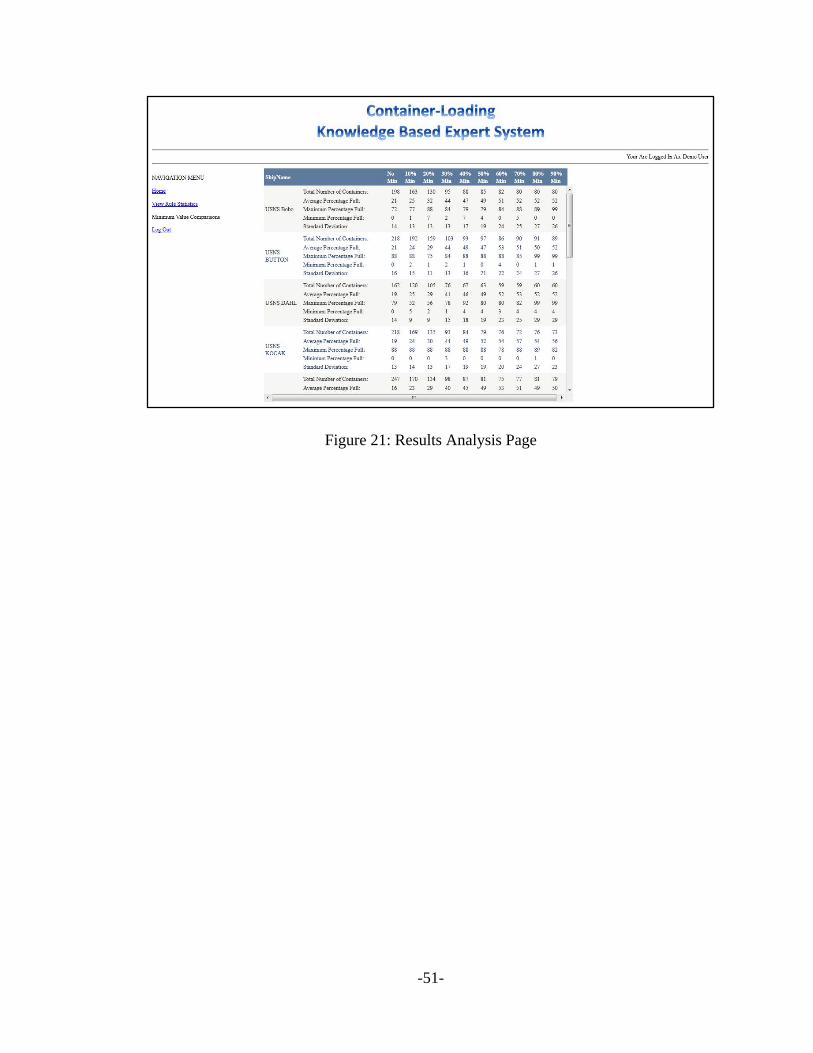
-51-
Figure 21: Results Analysis Page

-52-
Chapter 5
RESULTS ANALYSIS
This chapter will explain the results from comparing the container-loading knowledge-
based expert system with the historical data representing the manual container-loading
processes for thirteen ships loaded between 2008 and 2011. The first experiment that
will be discussed is the control experiment where the capabilities of the artificial
intelligence algorithm were tested against the historical data without using the inference
engine. The next experiment discussed is how the long-term minimum percentage to be
used by the inference engine when using historical data was determined. Finally, once
the minimum percentage was identified, the capabilities of the container-loading
knowledge-based expert system are compared to the historical data corresponding to the
ships loaded between 2008 and 2011.
5.1 Artificial Intelligence Control Experiment
Before testing the capabilities of the container-loading knowledge-based expert system as
a whole, the capabilities of the artificial intelligence were tested. The results discussed in
this section provided the baseline to see whether using historical data provides added
benefit in later sections. The user interface, as described in section 4.10, in which
problems are created allows for a problem to be solved exclusively using the artificial
intelligence. A problem was created for each of the thirteen ships for which historical
data was collected. Each problem represented the items that were loaded in the past
aboard each ship.

-53-
The container-loading knowledge-based expert system solved each problem. Figure 22
displays the raw data from the results of the artificial intelligence control experiment.
The historical data container count represents how many containers it took the container
loading experts to load all the equipment and supplies for each ship. The artificial
intelligence container count represents how many containers were needed for the
artificial intelligence to load the same number of equipment and supplies. The percent
decrease column shows the percent decreased by using the artificial intelligence for each
ship and is averaged at the bottom. The results show that the artificial intelligence can
function effectively in the problem domain because for each ship tested the artificial
intelligence was able to load the gear in fewer containers than the container-loading
experts. Using only the artificial intelligence, the container-loading knowledge-based
expert system loaded all the items for each ship into an average of 45.9% fewer
containers than the container-loading experts did manually. Figure 23 displays the data
from Figure 22 graphically, showing that the total container count for the artificial
intelligence was always lower than the results from the container-loading experts.

-54-
Figure 22: Artificial Intelligence Control Experiment Results
Figure 23: Artificial Intelligence Control Experiment Results Chart
In addition to reducing the number of containers, the average percentage full of each
container also increased. The historical data column in Figure 24 shows the average
percentage full of the containers loaded onto each ship by the container-loading experts.
Ship Name Historical Data Container Count
Artificial Intelligence Container Count
Percentage Decrease
!"#$%& 151 80 '()*+!"#$%, 171 90 '()'+!"#$%- 108 59 '.)'+!"#$%' 158 73 .-)/+!"#$%. 134 79 '&)*+!"#$%0 150 108 ,/)*+!"#$%( 61 34 '')-+!"#$%/ 174 92 '()&+!"#$%1 172 75 .0)'+!"#$%&* 74 32 .0)/+!"#$%&& 75 38 '1)-+!"#$%&, 115 73 -0).+!"#$%&- 125 71 '-),+
2345264 &,/)- 01). '.)1+
!"
#!"
$!"
%!"
&!"
'!!"
'#!"
'$!"
'%!"
'&!"
#!!"
()*+"'" ()*+"#" ()*+"," ()*+"$" ()*+"-" ()*+"%" ()*+"." ()*+"&" ()*+"/" ()*+"'!" ()*+"''" ()*+"'#" ()*+"',"
0*1234*567"8626"93:26*:;4"93<:2"
=4>?5*67"@:2;77*A;:5;"93:26*:;4"93<:2"
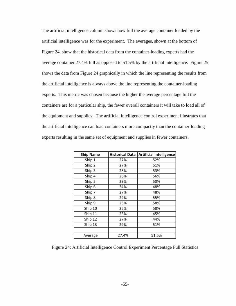
-55-
The artificial intelligence column shows how full the average container loaded by the
artificial intelligence was for the experiment. The averages, shown at the bottom of
Figure 24, show that the historical data from the container-loading experts had the
average container 27.4% full as opposed to 51.5% by the artificial intelligence. Figure 25
shows the data from Figure 24 graphically in which the line representing the results from
the artificial intelligence is always above the line representing the container-loading
experts. This metric was chosen because the higher the average percentage full the
containers are for a particular ship, the fewer overall containers it will take to load all of
the equipment and supplies. The artificial intelligence control experiment illustrates that
the artificial intelligence can load containers more compactly than the container-loading
experts resulting in the same set of equipment and supplies in fewer containers.
Figure 24: Artificial Intelligence Control Experiment Percentage Full Statistics
Ship%Name Historical%Data% Artificial%IntelligenceShip%1 27% 52%Ship%2 27% 51%Ship%3 28% 53%Ship%4 26% 56%Ship%5 29% 50%Ship%6 34% 48%Ship%7 27% 48%Ship%8 29% 55%Ship%9 25% 58%Ship%10 25% 58%Ship%11 23% 45%Ship%12 27% 44%Ship%13 29% 51%
Average 27.4% 51.5%

-56-
Figure 25: Artificial Intelligence Control Experiment Percentage Graph
5.2 Inference Engine Minimum Percentage Experiment
The next experiment conducted was to determine what the minimum percentage should
be for the inference engine when using historical data. The user interface, where
problems are created, was also configured to allow for any minimum value to be used for
testing purposes. For each of the thirteen ships, ten problems were created each with a
different minimum percentage starting at no minimum percentage and increasing by ten
percent up to ninety percent. Each problem was solved using the container-loading
knowledge-based expert system. In this experiment, the full capabilities of the system
were tested. The inference engine used historical data that was above the minimum
percentage until there were no rules left that could be applied. The artificial intelligence
then solved the rest of the problem.
The resulting container counts for each problem are shown in Figure 26. Each ship’s data
was loaded using the ten different minimum values represented by the column headers.
!"#
$!"#
%!"#
&!"#
'!"#
(!"#
)!"#
*!"#
+,-.#$# +,-.#%# +,-.#&# +,-.#'# +,-.#(# +,-.#)# +,-.#*# +,-.#/# +,-.#0# +,-.#$!# +,-.#$$# +,-.#$%# +,-.#$&#
1-2345-678#9737## :5;<6-78#=>3?88-@?>6?#

-57-
The number in the chart represents the number of containers it took the container-loading
knowledge-based expert system to load all the equipment and supplies for that ship. The
results in their raw form cannot be compared across different ships because each ship had
a different number of equipment and supplies loaded. Therefore, for each problem the
minimum container count across all ten problems was identified for each ship, shown as
the absolute minimum column of Figure 26. Each container count was then divided by
the absolute minimum value for that ship resulting in the percentage of the minimum
container count each total represents, shown in Figure 27. Now each total represents the
percentage of the minimum container count and the percentages can be compared across
different ships.
Figure 26: Container Counts for Minimum Percentage Experiment
Ship%Name No%Min 10%%Min 20%%Min 30%%Min 40%%Min 50%%Min 60%%Min 70%%Min 80%%Min 90%%Min Absolute%Min
Ship%1 198 163 130 95 88 85 82 80 80 80 80Ship%2 218 192 159 103 93 97 86 90 91 89 86Ship%3 162 120 105 76 67 63 59 59 60 60 59Ship%4 218 169 135 93 84 79 76 72 76 73 72Ship%5 247 170 134 98 87 81 75 77 81 79 75Ship%6 278 234 176 134 111 106 108 108 107 107 106Ship%7 102 85 58 42 38 35 35 32 34 35 32Ship%8 248 188 155 115 97 94 86 85 89 89 85Ship%9 214 183 148 101 88 83 76 70 78 75 70Ship%10 128 74 56 44 34 33 33 32 31 31 31Ship%11 92 74 52 45 38 37 35 37 39 38 35Ship%12 212 137 110 82 77 74 70 70 73 72 70Ship%13 196 155 119 89 80 74 69 70 71 69 69

-58-
Figure 27: Percentages of the Absolute Minimum Values
The percentages in Figure 27 that represent the absolute minimum container count for
each ship are those cells with one hundred percent. Any cell with a number greater than
one hundred percent represents a total that was greater than the absolute minimum for
that particular ship by the percentage in the cell. Figure 28 shows the data from Figure
27 in a graphical form in which the values decrease rapidly after the thirty percent
minimum threshold and reaches its minimum at the seventy percent minimum threshold.
Figure 29 graphs the averages for each minimum percentage, represented in the bottom
row of Figure 27, and provides a much clearer representation of the performance.
Ship%Name No%Min 10%%Min 20%%Min 30%%Min 40%%Min 50%%Min 60%%Min 70%%Min 80%%Min 90%%Min
Ship%1 247.5% 203.8% 162.5% 118.8% 110.0% 106.3% 102.5% 100.0% 100.0% 100.0%Ship%2 253.5% 223.3% 184.9% 119.8% 108.1% 112.8% 100.0% 104.7% 105.8% 103.5%Ship%3 274.6% 203.4% 178.0% 128.8% 113.6% 106.8% 100.0% 100.0% 101.7% 101.7%Ship%4 302.8% 234.7% 187.5% 129.2% 116.7% 109.7% 105.6% 100.0% 105.6% 101.4%Ship%5 329.3% 226.7% 178.7% 130.7% 116.0% 108.0% 100.0% 102.7% 108.0% 105.3%Ship%6 262.3% 220.8% 166.0% 126.4% 104.7% 100.0% 101.9% 101.9% 100.9% 100.9%Ship%7 318.8% 265.6% 181.3% 131.3% 118.8% 109.4% 109.4% 100.0% 106.3% 109.4%Ship%8 291.8% 221.2% 182.4% 135.3% 114.1% 110.6% 101.2% 100.0% 104.7% 104.7%Ship%9 305.7% 261.4% 211.4% 144.3% 125.7% 118.6% 108.6% 100.0% 111.4% 107.1%Ship%10 412.9% 238.7% 180.6% 141.9% 109.7% 106.5% 106.5% 103.2% 100.0% 100.0%Ship%11 262.9% 211.4% 148.6% 128.6% 108.6% 105.7% 100.0% 105.7% 111.4% 108.6%Ship%12 302.9% 195.7% 157.1% 117.1% 110.0% 105.7% 100.0% 100.0% 104.3% 102.9%Ship%13 284.1% 224.6% 172.5% 129.0% 115.9% 107.2% 100.0% 101.4% 102.9% 100.0%
Average 296.1% 225.5% 176.3% 129.3% 113.2% 108.2% 102.7% 101.5% 104.8% 103.5%

-59-
Figure 28: Graphical Percentages of the Absolute Minimum Values
Figure 29: Graph of Average Percentages of the Absolute Minimum
The lowest average value for the minimum value threshold for historical data is at
seventy percent. These results imply that the minimum values created by the system are
most often occurring with a minimum percentage of seventy percent for historical data.
100.0%
150.0%
200.0%
250.0%
300.0%
350.0%
400.0%
450.0%
No Min
10% Min
20% Min
30% Min
40% Min
50% Min
60% Min
70% Min
80% Min
90% Min
Ship 1
Ship 2
Ship 3
Ship 4
Ship 5
Ship 6
Ship 7
Ship 8
Ship 9
Ship 10
Ship 11
Ship 12
Ship 13
100.0%
150.0%
200.0%
250.0%
300.0%
350.0%
No Min
10% Min
20% Min
30% Min
40% Min
50% Min
60% Min
70% Min
80% Min
90% Min
Average

-60-
Seventy percent is where the optimal combination between the historical data and the
artificial intelligence exists. The artificial intelligence, as shown above in Figure 24, has
an average value of 51.5%. Therefore, when the minimum value is set at seventy percent
there are enough historical data rules used to increase the overall percentage full of the
containers before the artificial intelligence solves the rest of the problem. Increasing the
overall percentage full of each container leads to a lower container count. The problems
solved with minimum values above seventy percent did not have as many rules that could
be used from historical data and thus the artificial intelligence had to solve more of the
problem. Since the artificial intelligence averages loading containers 51.5% full, the
more of the problem the artificial intelligence had to solve the more the average
percentage full of the containers approached 51.5%. The improved methodology relies
on data warehousing to provide the ability to exceed the capabilities of the artificial
intelligence alone. The effectiveness of the data warehouse is minimized when the
minimum percentage for the inference engine is higher than seventy percent.
Figure 30 shows the average percentage full containers loaded for each problem solved
were. The problem corresponding to each ship was solved ten different times each with a
different minimum value and thus generated ten different percentages. The percentages
at sixty, seventy, and ninety percentages are all above the 51.5% average, as shown in
Figure 24, for the artificial intelligence by itself. Figure 31 graphically represents the
data from Figure 30. The percentage full peaks at seventy percent and thus explains why
seventy percent had the lowest container counts. Figure 32, which graphs the average of
all the percentages for each minimum value, shows similar results. The containers loaded
using seventy percent as the minimum value for historical data had the highest average

-61-
percentage full. Therefore, empirical data from this experiment, including both the
container counts and the average percentage full of containers, shows that the long term
minimum percentage that should be used for historical data is seventy percent.
Figure 30: Average Percentage Full of Containers
Figure 31: Graph of Percentage Full of Containers
Ship%Name No%Min 10%%Min 20%%Min 30%%Min 40%%Min 50%%Min 60%%Min 70%%Min 80%%Min 90%%MinShip%1 21% 25% 32% 44% 47% 49% 51% 52% 52% 52%Ship%2 21% 24% 29% 44% 49% 47% 53% 51% 50% 52%Ship%3 19% 25% 29% 41% 46% 49% 52% 53% 52% 52%Ship%4 19% 24% 30% 44% 49% 52% 54% 57% 54% 56%Ship%5 16% 23% 29% 40% 45% 49% 53% 51% 49% 50%Ship%6 18% 22% 29% 38% 47% 49% 48% 48% 48% 48%Ship%7 16% 19% 28% 39% 43% 47% 47% 51% 48% 47%Ship%8 20% 26% 32% 43% 52% 53% 58% 59% 56% 56%Ship%9 20% 24% 29% 43% 50% 53% 58% 63% 56% 58%Ship%10 14% 25% 33% 42% 55% 56% 56% 58% 60% 60%Ship%11 18% 23% 33% 38% 45% 47% 49% 47% 44% 45%Ship%12 15% 23% 29% 39% 41% 43% 45% 45% 43% 44%Ship%13 18% 23% 30% 41% 45% 49% 53% 52% 51% 53%
Average 18.1% 23.5% 30.2% 41.2% 47.2% 49.5% 52.1% 52.8% 51.0% 51.8%
0%
10%
20%
30%
40%
50%
60%
70%
No Min 10% Min
20% Min
30% Min
40% Min
50% Min
60% Min
70% Min
80% Min
90% Min
Ship 1
Ship 2
Ship 3
Ship 4
Ship 5
Ship 6
Ship 7
Ship 8
Ship 9
Ship 10
Ship 11
Ship 12
Ship 13

-62-
Figure 32: Averages of Percentage Full of Containers
5.3 Final Comparison
Once the capabilities of the artificial intelligence were identified and the optimal
minimum percentage to use for historical data was identified, the final comparison could
be conducted. The results from the tests with the minimum percentage of seventy percent
were compared to the historical data and against the artificial intelligence by itself. The
historical data container count was always higher than the container count for the
improved methodology, seen by comparing the historical data container count with the
improved methodology container count column in Figure 33. The improved
methodology performance, as shown in Figure 33 by the average percentage decrease for
the improved methodology, decreased the overall container counts needed to load each
ship by a greater margin than by strictly using the artificial intelligence. Therefore by
combining both historical data and artificial intelligence, a more optimal solution,
meaning loading the same number of equipment and supplies into a smaller number of
containers, was achieved in each case by the improved methodology. Figure 34 graphs
these results showing how the total container count for the improved methodology is
0.0%
10.0%
20.0%
30.0%
40.0%
50.0%
60.0%
No Min 10% Min
20% Min
30% Min
40% Min
50% Min
60% Min
70% Min
80% Min
90% Min
Average

-63-
always below the historical data container count and always below or equal to the
artificial intelligence container count.
Figure 33: Final Comparison Statistics
Figure 34: Final Comparison Graph
!"#$%&'() *#+,-.#/'0%1','%2-3,'#3).%2-43,
5.,#6#/#'0%73,)00#8)3/)%2-3,'#3).%2-43,
9)./)3,'8)%1)/.)'+)%:5.,#6#/#'0%73,)00#8)3/)%
;+%*#+,-.#/'0%1','<
7($.-;)=%>),"-=-0-8?%2-3,'#3).%2-43,%:@AB%
>#3#(4(%C'04)<
9)./)3,'8)%1)/.)+)%:7($.-;)=%>),"-=-0-8?%
;+%*#+,-.#/'0%1','<
!"#$%& &'& () *+,)- () *+,)-!"#$%. &+& /) *+,*- /) *+,*-!"#$%0 &)( '/ *',*- '/ *',*-!"#$%* &'( +0 '0,(- +. '*,*-!"#$%' &0* +/ *&,)- ++ *.,'-!"#$%1 &') &)( .(,)- &)( .(,)-!"#$%+ 1& 0* **,0- 0. *+,'-!"#$%( &+* /. *+,&- (' '&,&-!"#$%/ &+. +' '1,*- +) '/,0-!"#$%&) +* 0. '1,(- 0. '1,(-!"#$%&& +' 0( */,0- 0+ '),+-!"#$%&. &&' +0 01,'- +) 0/,&-!"#$%&0 &.' +& *0,.- +) **,)-
2345674 &.(,0 1/,' *',/- 1+,( *+,.-
0
20
40
60
80
100
120
140
160
180
Ship 1 Ship 2 Ship 3 Ship 4 Ship 5 Ship 6 Ship 7 Ship 8 Ship 9 Ship 10 Ship 11 Ship 12 Ship 13
Historical Data Container Count
Artificial Intelligence Container Count
Improved Methodology Container Count (70% Minimum Value)

-64-
The average percentage full of containers for each problem supports the same
conclusions. As shown in Figure 35, the average percentage full of each container is as
high or higher for each ship in the improved methodology as compared to both the
historical data and the artificial intelligence. The higher the average percentage full for
each container, the lower the overall container count will be. The average container from
historical data was 27.4% full, as shown in Figure 35. The average container from the
artificial intelligence control experiment was 51.5% full, which is a percentage increase
of 89.2%, as shown in Figure 35. The average container from using the container-
loading knowledge-based expert system with a minimum percentage of seventy percent
for historical data was 52.8% full, which was a percentage increase of 94.9%, also shown
in Figure 35. Figure 36 graphically represents the data from Figure 35. The line
corresponding to the improved methodology is always as high or higher than the artificial
intelligence and always higher than the historical data.
The artificial intelligence experiment led to a 45.9% reduction in the container count, as
shown in Figure 33. However, by combining historical data and artificial intelligence,
the container-loading knowledge-based expert system was able to reduce the container
count by 47.2%, also shown in Figure 33. Corresponding results were found when
analyzing the average percentage full containers were loaded by each method. The
artificial intelligence led to an increase in the average percentage full of the containers
loaded by 89.7%, as shown in Figure 35. However, the improved methodology led to an
increase in the average percentage full of 94.9%, also shown in Figure 35. The improved
methodology employed in the container-loading knowledge-based expert system
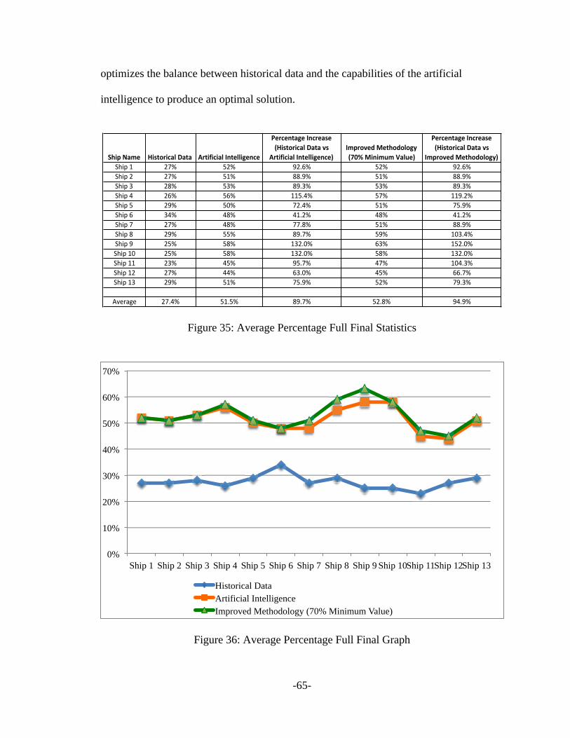
-65-
optimizes the balance between historical data and the capabilities of the artificial
intelligence to produce an optimal solution.
Figure 35: Average Percentage Full Final Statistics
Figure 36: Average Percentage Full Final Graph
!"#$%&'() *#+,-.#/'0%1','% 2.,#3#/#'0%45,)00#6)5/)
7)./)5,'6)%45/.)'+)%8*#+,-.#/'0%1','%9+%
2.,#3#/#'0%45,)00#6)5/):4($.-9);%<),"-;-0-6=%8>?@%<#5#(A(%B'0A):
7)./)5,'6)%45/.)'+)%8*#+,-.#/'0%1','%9+%
4($.-9);%<),"-;-0-6=:!"#$%& '() *') +',-) *') +',-)!"#$%' '() *&) ..,+) *&) ..,+)!"#$%/ '.) */) .+,/) */) .+,/)!"#$%0 '-) *-) &&*,0) *() &&+,')!"#$%* '+) *1) (',0) *&) (*,+)!"#$%- /0) 0.) 0&,') 0.) 0&,')!"#$%( '() 0.) ((,.) *&) ..,+)!"#$%. '+) **) .+,() *+) &1/,0)!"#$%+ '*) *.) &/',1) -/) &*',1)!"#$%&1 '*) *.) &/',1) *.) &/',1)!"#$%&& '/) 0*) +*,() 0() &10,/)!"#$%&' '() 00) -/,1) 0*) --,()!"#$%&/ '+) *&) (*,+) *') (+,/)
2345674 '(,0) *&,*) .+,() *',.) +0,+)
0%
10%
20%
30%
40%
50%
60%
70%
Ship 1 Ship 2 Ship 3 Ship 4 Ship 5 Ship 6 Ship 7 Ship 8 Ship 9 Ship 10 Ship 11 Ship 12 Ship 13
Historical Data Artificial Intelligence Improved Methodology (70% Minimum Value)

-66-
Chapter 6
CONCLUSIONS AND FUTURE WORK
In this chapter, conclusions based on the results of the previous chapter will be discussed
in section 6.1. Discussions about future work will be discussed in section 6.2.
6.1 Conclusions
Knowledge-based expert systems can drastically reduce the amount of time necessary to
complete complex tasks in a particular domain when implemented properly. However,
there are significant problems that can arise during the implementation of a knowledge-
based expert system that can prevent the system from ever becoming functional.
Furthermore, the post implementation maintenance requirements of a knowledge-based
expert system can be difficult and time consuming. Only by identifying and mitigating
these risks can a knowledge-based expert system be successfully implemented and
maintained.
An improved methodology for creating and maintaining knowledge-based expert systems
was introduced in this thesis. The improved methodology streamlines the knowledge
acquisition process by mining historical data to augment the interviews conducted by the
knowledge engineer. The historical data provide a strong starting point for the
knowledge base, which is transformed into a data warehouse to provide the inference
engine fast access to the historical data. Furthermore, artificial intelligence is
incorporated into the knowledge-based expert system in order to suggest new rules that
can be added to the knowledge base. The suggested rules will allow the knowledge-
-67-
based expert system to completely solve problems that cannot be solved given the
information contained within the knowledge base. The incorporation of the artificial
intelligence removes the need for a manual knowledge acquisition module and thus
reduces the resource requirements for maintaining the knowledge-based expert system
after its initial implementation.
The improved methodology was tested by creating a knowledge-based expert system for
a container-loading process. Container-loading experts were interviewed to discuss their
processes. The transportation system where the data was recorded by the container-
loading experts was mined for the historical data from thirteen ships loaded between
2008 and 2011. A data warehouse was created to serve as the knowledge base to store
historical data. The inference engine was created in order to pass partially completed
solutions to the artificial intelligence. The artificial intelligence then constructed the
rules that needed to be added to the knowledge base in order to complete the solution.
In order to test the container-loading knowledge-based expert system, several
experiments were conducted. The first experiment tested the capabilities of the artificial
intelligence algorithm. The historical data from each of the thirteen ships loaded by the
container-loading experts between 2008 and 2011 were turned into distinct problems in
the system. Each problem was then solved by the artificial intelligence without the use of
the inference engine or any historical data. The artificial intelligence was able to load all
the items from each ship with an average of 45.9% less containers than the container-
loading experts had done in the past, as shown in Figure 27. The average percentage full
the containers loaded by the artificial intelligence was 51.5% as opposed to 27.4% by the
container-loading experts, as shown in Figure 29. This experiment provided a control

-68-
baseline for later experiments to test the impact of using both historical data and artificial
intelligence.
The second experiment was designed to identify what the long-term minimum value
should be for using historical data. Each rule stored in the knowledge base represents
some percentage of a fully loaded container. The inference engine was created so that it
would not use any rules below the minimum percentage set before the problem was
solved. For each of the thirteen ships, ten problems were created each with a different
minimum value starting with no minimum value and increasing by ten percent up to
ninety percent. Each problem was then solved independently so the results could be
compared. The results for the problems solved with a minimum value of seventy percent
yielded the lowest container counts on average and also yielded the highest average
percentage full for the containers loaded. Therefore, seventy percent was selected to be
the long-term minimum value for the inference engine to use when selecting historical
data.
The final experiment compared the results from the container-loading knowledge-based
expert system using a minimum value of seventy percent with the results from the
artificial intelligence control experiment and the historical results. The container-loading
knowledge-based expert system was able to reduce the total number of containers needed
to load the thirteen ships by 47.2%, which was a greater reduction than the artificial
intelligence alone. Furthermore, the containers were on average 52.8% full, which was
greater than the artificial intelligence alone and greater than the historical results from the
container-loading experts. These results show that by utilizing both historical data and

-69-
artificial intelligence a more optimal solution can be created than by using either one of
them independently.
The most important part of the improved methodology was to identify where the optimal
combination of historical data and artificial intelligence existed. The testing phase of the
improved methodology is thus critical to a successful implementation. If the optimal
balance is achieved then the knowledge-based expert system can produce optimal
solutions while reducing the maintenance requirements of the knowledge base.
6.2 Future Work
Future experiments with the improved methodology for the knowledge-based expert
systems need to be conducted in other problem domains. Other areas within the shipping
industry could also be analyzed, for example this methodology could be implemented to
load a ship with vehicles. Also, the a knowledge-based expert system could be created to
create load plans for ships and integrated with Wilson’s algorithm, as described in
Chapter 2 [Wilson99]. By using the improved methodology in other domains, a more
defined process for establishing the bounds for the inference engine using historical data
could be achieved.
The impact of historical data when coupled with artificial intelligence is an area that
could be improved. Fine tuning the inference engine and possibly modifying the artificial
intelligence could potentially allow the historical data to provide a more significant
impact beyond the capabilities of the artificial intelligence alone. Given the amount of
data that is now stored and archived by organizations, it is important to investigate
improved ways of utilizing the data to improve productivity and quality.

-70-
REFERENCES [Aniba09] Aniba, M., S. Siguenza, A. Friedrich, F. Plewniak, O. Poch, A. Marchler-Bauer, and J.D.
Thompson. “Knowledge-based expert systems and a proof-of-concept case study for multiple sequence alignment construction and analysis,” Briefings in Bioinformatics, 10, 1 (2009), pp. 11-23.
[Bobrow86] Bobrow, D., S. Mittal, and M. Stefik. “Expert Systems: Perils and Promise,” ACM
Common, 29, 9 (September 1986), pp. 880-894. [Dabbaghchi97] Dabbaghchi, I., R. Christie, G. Rosenwald, and C. Liu. “AI Application Areas in Power
Systems,” IEEE Expert: Intelligent Systems and Their Applications, 12, 1 (January 1997), pp. 58-66.
[Dalal11] Dalal, M., and N. Harale. “A survey on clustering in data mining,” Proceedings of the
International Conference & Workshop on Emerging Trends in Technology (ICWET '11), 38 (2011), pp. 559-562.
[El-Najdawi93] El-Najdawi, M., and A. Stylianou. “Expert support systems: Integrating AI
Technologies,” Communications of the ACM, 36, 12 (December 1993), pp. 55-65. [Fan06] Fan, W., J. McCloskey, and P. Yu. “A general framework for accurate and fast regression
by data summarization in random decision trees,” Proceedings of the 12th ACM SIGKDD international conference on Knowledge discovery and data mining, 12 (2006), pp. 136-146.
[Fayyad96] Fayyad, U., G. P.-Shapiro, and P. Smyth. “From Data Mining to Knowledge Discovery
in Databases,” AI Magazine, 17(3) (Fall 1996), pp. 37-54. [Forsythe89] Forsythe, D., and B. Buchanan. "Knowledge acquisition for expert systems: some pitfalls
and suggestions," Systems, Man and Cybernetics, IEEE Transactions, 19, 3 (May 1989), pp.435-442.

-71-
[Gardner98] Gardner, S. “Building the Data Warehouse,” Communications of the ACM, 41, 9
(September 1998), pp. 52-60. [Giarratano89] Giarratano, J., and G. Riley. Expert Systems: Principles and Programming. PWS-Kent
Publishing Company, Boston, 1989. [Golabchi08] Golabchi, M. “A knowledge-based expert system for selection of appropriate structural
systems for large spans,” Asian Journal of Civil Engineering Building and Housing, 9, 2 (2008), pp. 179–191.
[Grosan11] Grosan, C., and A. Abraham. Intelligent Systems: A Modern Approach, Springer-Verlag,
Berlin, 2011. [Han12] Han, J., M. Kamber, and J. Pei. Data Mining Concepts and Techniques. Morgan
Kaufman Publishers, Elsevier Inc, Waltham, Massachusetts, 2012. [Hanson90] Hanson , E., M. Chaabouni, C. Kim, Y. Wang. “A Predicate Matching Algorithm for
Database Rule Systems,” Proceedings of the 1990 ACM SIGMOD international conference on Management of data, 90 (May 1990), pp. 271-280.
[Hardaway90] Hardaway, D., and R. Willi. “A Review of Barriers to Expert System Diffusion,”
Proceedings of the 1990 ACM SIGBDP conference on Trends and directions in expert systems, SIGBDP 90, pp. 619-639.
[He10] He, K., and W. Huang. “A caving degree based flake arrangement approach for the
container loading problem,” Computers & Industrial Engineering, 59 (2010), pp. 344-351.
[Hoplin90] Hoplin, H., and S. Erdman. “Expert Systems: An Expanded Field of Vision for
Business,” Proceedings of the 1990 ACM SIGBDP conference on Trends and directions in expert systems, SIGBDP (1990), pp. 1-16.
[Huang07] Huang, W. and K. He. “A caving degree approach for the single container loading
problem,” European Journal of Operational Research, 196 (2009), pp. 93-101.

-72-
[Khan02] Khan, S., K. Li, F. Manning, AND M. Akbar. “Solving the knapsack problem for
adaptive multimedia systems,” Studia Informatica Universalis, 2, 1 (2002), 157–178, 2002.
[Kimball94] Kimball, R., K. Strehlo. “Why decision support fails and how to fix it.” Datamation, 40,
11 (June 1994), pp. 40-43. [Kiper92] Kiper, J., “Structural testing of rule-based expert systems,” ACM Trans. Software
Engineering. Methodology, 1, 2 (April 1992), pp. 168-187. [La Salle90] La Salle, A, and L. Medsker. “The Expert System Life Cycle: What Have We Learned
From Software Engineering?” Proceedings of the 1990 ACM SIGBDP conference on Trends and directions in expert systems, SIGBDP (1990), pp. 17-26.
[Levene03] Levene, M., and G. Loizou. “Why is the snowflake schema a good data warehouse
design?” Information Systems, 28, 3 (May 2003), pp. 225-240. [Lutu02] Lutu, P. “An integrated approach for scaling up classification and prediction algorithms
for data mining.” ACM International Conference Proceeding Series, 30 (2002), pp. 110-117.
[Mattos03] Mattos, E., H. Hoeschl, M. Ribeiro, and C. Bueno. “A Knowledge Base for Automatic
Capitulation in Expert System,” Proceedings of the 9th international conference on Artificial intelligence and law, ICAIL (2003), pp. 99-100.
[Mertens04] Mertens, S., M. Rosu, and Y. Erdani. “An intelligent dialogue for online rule based
expert systems,” Proceedings of the 9th international conference on intelligent user interfaces, IUI, (2004), pp. 280-282.
[Millinton09] Millington, I., and J. Funge. Artificial Intelligence For Games, Second Edition, Elsevier
Inc, Burlington, MA, 2009. [O’Leary98] O'Leary, D. "Using AI in knowledge management: Knowledge Bases and ontologies,"
Intelligent Systems and their Applications, IEEE, 13, 3 (May 1998), pp. 34-39.

-73-
[Orriols-Puig08] Orriols-Puig, A., J. Casillas, and E. Bernadó-Mansilla. “First approach toward on-line
evolution of association rules with learning classifier systems,” Proceedings of the 2008 GECCO conference companion on Genetic and evolutionary computation, GECCO (2008), pp. 2031-2038.
[Pisinger05] Pisinger, D. “Where are the hard knapsack problems?” Computers & Operations
Research, 32, e 9 (September 2005), pp. 2271-2284. [Romero07] Romero, C., S. Ventura, and E. García. “Data Mining in Course Management Systems:
Moodle Case Study and Tutorial,” Computers & Education, 51, 1 (August 2008), pp. 368-384.
[Russell03] Russell, S., and P. Norvig. Artificial Intelligence A Modern Approach, Second Edition.
Pearson Education, Inc., Upper Saddle River, NJ, 2003. [Skoutas11] Skoutas, D., and A. Simitsis. "Ontology-Based Conceptual Design of ETL Processes for
Both Structured and Semi-Structured Data, " International Journal on Semantic Web and Information Systems, 3, 4 (2007), pp. 1-24.
[Stewart05] Stewart, J. Single Variable Calculus Concepts & Contexts. Thomson Learning, Inc,
Belmont, CA, 2005. [Stonebraker92] Stonebraker, M. “The Integration of Rule Systems and Database Systems,” IEEE
Transactions on Knowledge and Data Engineering, 4, 5 (October 1992), pp. 415-423. [Teorey06] Teorey, T., S. Lightstone, and T. Nadeau. Database Modeling and Design, Fourth
Edition, Morgan Kaufman Publishers, Elsevier Inc, Amsterdam, 2006. [Teorey11] Teorey, T., S. Lightstone, T. Nadeu, and H.V Jagadish. Database Modeling and Design:
Logical Design, Fifth Edition, Morgan Kaufman Publishers, Elsevier Inc, Burlington, MA, 2011.
[Vassiliadis02] Vassiliadis, P., A. Simitsis, and S. Skiadopoulos. “Conceptual modeling for ETL
Processes,” Proceedings of the 5th ACM international workshop on Data Warehousing and OLAP, DOLAP (2002), pp. 14-21.

-74-
[Wagner90] Wagner, W. “Issues in Knowledge Acquisition,” Proceedings of the 1990 ACM
SIGBDP conference on Trends and directions in expert systems, SIGBDP (1990), pp. 247-261.
[Whelan96] Whelan, P., and B. Batchelor. “Automated Packing Systems – A Systems Engineering
Approach,” IEEE Transactions on Systems, Man, and Cybertronics – Part A, 26, 5 (Septmeber 1996), pp. 533-544.
[Wilson99] Wilson, I.D., and P. Roach. “Principals of Combinatorial Optimization Applied to
Container-Ship Planning,” Journal of Heuristics, 5 (1999), pp. 403-418. [Zimbrão03] Zimbrão, G., R. Miranda, J. Souza, M. Estolano, and F. Neto. “Enforcement of Business
Rules in Relational Databases Using Constraints,” Proceedings of XVIII Simposio Brasileiro de Bancos de Dados/SBBD (2003), pp. 129–141.

-75-
Appendix A
EXAMPLE OF USER INTERFACE SOURCE CODE The user interfaces were created as web pages using Microsoft .Net framework 4.0. The source code for these web pages is split into two files. The first file with the extension “.aspx” is similar to a standard HTML file where the layout of the web page is defined. The second file with the extension “.aspx.vb” is where the code is created for specific events for the web page.
A.1 ViewSolutions.aspx
Description: This file is where solutions can be created and viewed in the system. The web pages display the solutions using standard active server page (ASP) controls which when rendered to the client are transformed into standard HTML. <%@ Page Title="" Language="vb" AutoEventWireup="false" MasterPageFile="~/SiteMaster.Master" CodeBehind="ViewSolution.aspx.vb" Inherits="ExpertSystem.ViewSolution" %> <%@ Register Assembly="AjaxControlToolkit" Namespace="AjaxControlToolkit" TagPrefix="asp" %> … <asp:Content ID="Content2" ContentPlaceHolderID="ContentPlaceHolder1" runat="server"> … <asp:GridView ID="gvSolution" runat="server" AutoGenerateColumns="False" > <Columns> <asp:TemplateField HeaderText="Solution Description"> <ItemTemplate> <asp:Panel ID="pHeader" runat="server" cssclass="collapsePanelHeader"> <table width="100%" > <tr> <td style="text-align:left; width:80%">
Container Number: <asp:Label ID="lblContainerNumber" runat="server" Text="Label" ondatabinding="lblContainer_DataBinding"></asp:Label>
Rule ID: <asp:Label ID="lblRuleGuid" runat="server" Text="Label"></asp:Label
Percentage Full: <asp:Label ID="lblPercentageFull" runat="server" Text="Label"></asp:Label>
</td> <td style="text-align:right; width:20%">
<asp:Label ID="lblHeader" runat="server" Text="Label"></asp:Label> <asp:Image ID="imgToggle" runat="server" ImageUrl="Images/collapse.jpg" />

-76-
</td> </tr> </table> </asp:Panel> <asp:Panel ID="pContent" runat="server" CssClass="collapsePanel"> <asp:GridView ID="gvChildItems" runat="server"> </asp:GridView> </asp:Panel> <asp:CollapsiblePanelExtender ID="CollapsiblePanelExtender1" runat="server"
CollapseControlID="pHeader" Enabled="True" ExpandControlID="pHeader" TextLabelID="lblHeader" TargetControlID="pContent" CollapsedImage="~/Images/expand.jpg" ExpandedImage="~/Images/collapse.jpg" CollapsedText="Show Details..." ExpandedText="Hide Details..." ImageControlID="imgToggle" Collapsed="True" >
</asp:CollapsiblePanelExtender> </ItemTemplate> </asp:TemplateField> </Columns> <HeaderStyle HorizontalAlign="Left" /> </asp:GridView> <br /> … </asp:Content>
A.2 ViewSolutions.aspx.vb
Description: ViewSolutions.aspx.vb contains the code that is executed on the different events created by ViewSolutions.aspx. Also, calls to the business layer are initiated from this page. This class contains the code that calls the inference engine to start solving a problem and the artificial intelligence to complete the problem if necessary. Imports System.Data.SqlClient Partial Public Class ViewSolution Inherits System.Web.UI.Page Public MyInfEngine As InferenceEngine Public MyAICONT As ContainerLoadingAI Public MyPublicSolution As Solution Public mytype As String
Protected Sub Page_Load(ByVal sender As Object, ByVal e As System.EventArgs) Handles Me.Load Try If Not IsPostBack Then Dim cnsql As SqlConnection = New SqlConnection(System.Web.Configuration.WebConfigurationManager.ConnectionStrings("ES").ToString) cnsql.Open() Dim cmsql As New SqlCommand cmsql.Connection = cnsql cmsql.CommandType = CommandType.StoredProcedure cmsql.CommandText = "CheckSolutionExists"

-77-
Dim myGUID As New Guid(Request.QueryString("id")) cmsql.Parameters.Add("@GUID", SqlDbType.UniqueIdentifier) cmsql.Parameters("@GUID").Value = myGUID Dim count As Integer = cmsql.ExecuteScalar If count = 1 Then LoadSolution() mytype = "Load" Else mytype = "Create" cmsql = New SqlCommand cmsql.Connection = cnsql cmsql.CommandType = CommandType.StoredProcedure cmsql.CommandText = "UseHistoricalData" cmsql.Parameters.Add("@ProblemId", SqlDbType.UniqueIdentifier) cmsql.Parameters("@ProblemId").Value = myGUID Dim UseHistoricalData As Boolean = cmsql.ExecuteScalar Dim problem As New Problem(Request.QueryString("id")) Dim rules As New RuleCollection(UseHistoricalData, problem.Min) Dim myinferenceEngine As New InferenceEngine(rules, problem, UseHistoricalData) Dim completeSoultion As Boolean = myinferenceEngine.CreateSolution MyInfEngine = myinferenceEngine gvSolution.DataSource = myinferenceEngine.GetContainerTablefromSolution gvSolution.DataBind() Session.Add("myinfeng", myinferenceEngine) If Not completeSoultion Then gvUnspreadItems.DataSource = myinferenceEngine.GetUnspreadItemsTablefromSolution gvUnspreadItems.DataBind() lblUnspreadItems.Visible = True bCreateRules.Visible = True lblSolutionInfo.Text = "A Complete Solution could not be created using the existing rules. The items remaining are shown below. Additional rules can be generated automatically by clicking the generate rules button" lblSolutionInfo.Visible = True Else bSave.Visible = True lblSolutionInfo.Text = "A Complete Solution was generated using the existing rules. The data can be saved for future use by clicking the save button" lblSolutionInfo.Visible = True End If End If cnsql.Close() End If Catch ex As Exception Throw New Exception(ex.toString) End Try End Sub … Protected Sub bCreateRules_Click(ByVal sender As Object, ByVal e As EventArgs) Handles bCreateRules.Click

-78-
Try MyInfEngine = CType(Session("myinfeng"), InferenceEngine) Dim myAI As New ContainerLoadingAI(MyInfEngine.GetUnspreadItems) MyAICONT = myAI Dim test As Integer = myAI.UnspreadTotals myAI.GenerateRules() gvNewRules.DataSource = myAI.ReturnContainerInfoAsTable gvNewRules.DataBind() Session.Add("myAI", myAI) lblSaveAllRules.Visible = True lblRulesGenerationInfo.Visible = True bCreateRules.Visible = False Catch ex As Exception
Throw New Exception(ex.toString) End Try End Sub … End Class

-79-
Appendix B
EXAMPLE OF BUSINESS LAYER SOURCE CODE Descriptions: The business layer was designed to hold all the logic for the system. The classes created in the business later were designed to represent the different major components of the system, including the inference engine and the artificial intelligence. A small example of the artificial intelligence is shown below. Public Class ContainerLoadingAI Private myUnspreadItems As Collection Private myContainers As Collection Private myGroupedNSNlookup As Collection Public Sub New(ByVal UnspreadItems As Collection) myUnspreadItems = UnspreadItems myContainers = New Collection myGroupedNSNlookup = New Collection End Sub … Public Sub GenerateRules() Dim myContainerCount As Integer = 0 Dim itemsLoaded As Integer = 0 Dim myGUID As New Guid Dim myContainer As Container Dim ItemHasBeenLoaded As Boolean = False Dim ruleUsedAgain As Boolean = False GroupUnspreadItems() While ItemsRemain() Dim itemloaded As Boolean = False ruleUsedAgain = False If Not ItemHasBeenLoaded Then If myContainerCount > 0 Then myContainers.Add(myContainer) Dim NSNmappings As New Collection While TryRuleAgain(myContainer, NSNmappings, itemsLoaded) myContainerCount += 1 ruleUsedAgain = True Dim NewContainer As New Container NewContainer = myContainer.Copy() NewContainer.UpdateItemsNSN(NSNmappings, myGroupedNSNlookup) NewContainer.GetContainerNumber = myContainerCount myContainers.Add(NewContainer) NSNmappings.Clear()

-80-
NSNmappings = New Collection End While End If myContainerCount += 1 myGUID = Guid.NewGuid If Not ItemsRemain() Then Exit While End If myContainer = New Container(myContainerCount, myGUID.ToString, False) myContainer.SetDimensions(240, 96, 96) End If Dim bestItem As ThreeDimensional_Object Dim bestTotal As New AI_Calculation Dim cornercount As Integer = 1 For Each currentCorner As Coordinate In myContainer.Corners If currentCorner.IsActive Then … For Each currentItem As Child In myUnspreadItems
… If currentItem.QTY > 0 Then 'Check to see if the corner has a height > 0 and if item can be stacked If (currentCorner.Z_Coordinate > 0 And currentItem.Stack) Or currentCorner.Z_Coordinate = 0 Then 'Check Configuration 1 Dim testItem As New ThreeDimensional_Object(currentItem.Length, currentItem.Width, currentItem.Height, currentItem.NSN, False) testItem.SetCoordinateUsingMin(currentCorner) If myContainer.ItemCanBeLoaded(testItem) Then itemloaded = True Dim currentCalculation As New AI_Calculation(myContainer, testItem) If currentCalculation.IsGreater(bestTotal) Then bestItem = testItem bestTotal = currentCalculation End If End If If currentItem.Rotate Then 'Check Configuration 2 testItem = New ThreeDimensional_Object(currentItem.Length, currentItem.Height, currentItem.Width, currentItem.NSN, False) testItem.SetCoordinateUsingMin(currentCorner) If myContainer.ItemCanBeLoaded(testItem) Then itemloaded = True Dim currentCalculation As New AI_Calculation(myContainer, testItem) If currentCalculation.IsGreater(bestTotal) Then bestItem = testItem bestTotal = currentCalculation End If End If 'Check Configuration 3 testItem = New ThreeDimensional_Object(currentItem.Height, currentItem.Length, currentItem.Width, currentItem.NSN, False)

-81-
testItem.SetCoordinateUsingMin(currentCorner) If myContainer.ItemCanBeLoaded(testItem) Then itemloaded = True Dim currentCalculation As New AI_Calculation(myContainer, testItem) If currentCalculation.IsGreater(bestTotal) Then bestItem = testItem bestTotal = currentCalculation End If End If 'Check Configuration 4 testItem = New ThreeDimensional_Object(currentItem.Height, currentItem.Width, currentItem.Length, currentItem.NSN, False) testItem.SetCoordinateUsingMin(currentCorner) If myContainer.ItemCanBeLoaded(testItem) Then itemloaded = True Dim currentCalculation As New AI_Calculation(myContainer, testItem) If currentCalculation.IsGreater(bestTotal) Then bestItem = testItem bestTotal = currentCalculation End If End If 'Check Configuration 5 testItem = New ThreeDimensional_Object(currentItem.Width, currentItem.Length, currentItem.Height, currentItem.NSN, False) testItem.SetCoordinateUsingMin(currentCorner) If myContainer.ItemCanBeLoaded(testItem) Then itemloaded = True Dim currentCalculation As New AI_Calculation(myContainer, testItem) If currentCalculation.IsGreater(bestTotal) Then bestItem = testItem bestTotal = currentCalculation End If End If 'Check Configuration 6 testItem = New ThreeDimensional_Object(currentItem.Width, currentItem.Height, currentItem.Length, currentItem.NSN, False) testItem.SetCoordinateUsingMin(currentCorner) If myContainer.ItemCanBeLoaded(testItem) Then itemloaded = True Dim currentCalculation As New AI_Calculation(myContainer, testItem) If currentCalculation.IsGreater(bestTotal) Then bestItem = testItem bestTotal = currentCalculation End If End If End If End If End If Next
… Next 'if an item has been selected, load it If bestTotal.HasBeenSet Then Dim newitemToAdd As New ThreeDimensional_Object newitemToAdd = SelectGroupedItem(bestItem) myContainer.Load3DChild(newitemToAdd)

-82-
… ItemHasBeenLoaded = True Else ItemHasBeenLoaded = False End If End While If ItemHasBeenLoaded And Not ruleUsedAgain Then myContainers.Add(myContainer) End If End Sub … End Class

-83-
Appendix C
EXAMPLE OF DATA ACCESS LAYER SOURCE CODE Description: The code in the data access layer was designed to interact with the database and data warehouse through stored procedures. The objects created by the classes in the data access layer were designed to facilitate logical separations between objects within the database and data warehouse. Imports System.Data.SqlClient Imports System.Data Public Class Container Private containerID As Integer Private childItems As Collection Private ruleID As String Private mylength_X As Integer Private mywidth_Y As Integer Private myheight_Z As Integer Private myCorners As Collection Private mynewRuleID As Integer Private isCopy As Boolean Private myTotalVolume As Integer … Public Sub Load3DChild(ByVal child As ThreeDimensional_Object) Dim newCoord As Coordinate Dim objectCorner As Coordinate = child.MinCoordinate childItems.Add(child) 'remove the corner used to store this child For i As Integer = 1 To myCorners.Count Dim mycorner As Coordinate = CType(myCorners(i), Coordinate) If mycorner.IsEqual(child.MinCoordinate) Then myCorners.Remove(i) Exit For End If Next 'add the seven new corners for the new object newCoord = New Coordinate(objectCorner.X_Coordinate + child.Length, objectCorner.Y_Coordinate, objectCorner.Z_Coordinate) myCorners.Add(newCoord) newCoord = New Coordinate(objectCorner.X_Coordinate + child.Length, objectCorner.Y_Coordinate + child.Width, objectCorner.Z_Coordinate) myCorners.Add(newCoord)

-84-
newCoord = New Coordinate(objectCorner.X_Coordinate + child.Length, objectCorner.Y_Coordinate + child.Width, objectCorner.Z_Coordinate + child.Height) myCorners.Add(newCoord) newCoord = New Coordinate(objectCorner.X_Coordinate + child.Length, objectCorner.Y_Coordinate, objectCorner.Z_Coordinate + child.Height) myCorners.Add(newCoord) newCoord = New Coordinate(objectCorner.X_Coordinate, objectCorner.Y_Coordinate + child.Width, objectCorner.Z_Coordinate) myCorners.Add(newCoord) newCoord = New Coordinate(objectCorner.X_Coordinate, objectCorner.Y_Coordinate + child.Width, objectCorner.Z_Coordinate + child.Height) myCorners.Add(newCoord) newCoord = New Coordinate(objectCorner.X_Coordinate, objectCorner.Y_Coordinate, objectCorner.Z_Coordinate + child.Height) myCorners.Add(newCoord) updateCorners() End Sub … Public Sub SaveContainer() Dim mydt As DataTable = Me.GetContainerDetailAsTable Dim cnsql As New SqlConnection(System.Web.Configuration.WebConfigurationManager.ConnectionStrings("ES").ToString) cnsql.Open() Dim myGUID As New Guid(ruleID) Try Dim cmSQL As New SqlCommand For Each myrow As DataRow In mydt.Rows cmSQL = New SqlCommand cmSQL.CommandType = CommandType.StoredProcedure cmSQL.CommandText = "InsertRule" cmSQL.Connection = cnsql cmSQL.Parameters.Add("@GUID", SqlDbType.UniqueIdentifier) cmSQL.Parameters("@GUID").Value = myGUID cmSQL.Parameters.Add("@NSN", SqlDbType.Char) cmSQL.Parameters("@NSN").Value = myrow("NSN") cmSQL.Parameters.Add("@QTY", SqlDbType.Int) cmSQL.Parameters("@QTY").Value = CInt(myrow("QTY")) cmSQL.Parameters.Add("@UserName", SqlDbType.VarChar) cmSQL.Parameters("@UserName").Value = HttpContext.Current.User.Identity.Name.ToString cmSQL.ExecuteNonQuery() Next cmsql = New SqlCommand cmSQL.CommandType = CommandType.StoredProcedure cmSQL.CommandText = "UpdateVolume"

-85-
cmSQL.Connection = cnsql cmSQL.Parameters.Add("@GUID", SqlDbType.UniqueIdentifier) cmSQL.Parameters("@GUID").Value = myGUID cmSQL.ExecuteNonQuery() Catch ex As Exception Throw New Exception(ex.toString) Finally cnsql.Close() End Try End Sub … End Class

-86-
Appendix D
EXAMPLE OF STORED PROCEDURES Description: Stored procedures were used for all database and data warehouse queries. Below are examples of stored procedures that were called by the data access layer. -- ============================================= -- Author: Lucien Millette -- Create date: 8Dec2010 -- Description: Inserts a new problem with inputted parameters -- ============================================= CREATE PROCEDURE [dbo].[InsertProblem] -- Input Parameters @Name varchar(50), @UseHistoricalData bit, @MinimumPercentage int AS BEGIN -- SET NOCOUNT ON added to prevent extra result sets from -- interfering with SELECT statements. SET NOCOUNT ON; INSERT INTO [ProblemInfo] ([GUID] ,[Name] ,[CreatedOn] ,[UseHistoricalData] ,[MinimumPercentage]) VALUES (NEWID() ,@Name ,CURRENT_TIMESTAMP ,@UseHistoricalData ,@MinimumPercentage) END -- ============================================= -- Author: Lucien Millette -- Create date: 7Jan2011 -- Description: Inserts a part of a rule created by the AI -- ============================================= CREATE PROCEDURE [dbo].[InsertRule] -- Input Parameters @GUID uniqueidentifier, @NSN char(13), @QTY int, @UserName varchar(30)

-87-
AS BEGIN -- SET NOCOUNT ON added to prevent extra result sets from SET NOCOUNT ON; Declare @ID integer; Declare @CurrentTime datetime; Declare @Minute int; Declare @Hour int; Declare @Day int; Declare @Month int; Declare @Year int; Select @CurrentTime = CURRENT_TIMESTAMP if not exists (select Time_ID from TimeDimension where Time_ID = @CurrentTime) Begin insert into TimeDimension values (
@CurrentTime, DatePart(MINUTE, current_timestamp), DatePart(HOUR, current_timestamp), DatePart(DAY, current_timestamp), DatePart(Month, current_timestamp), DatePart(YEAR, current_timestamp))
End if exists (Select * from RuleFactTable where GUID = @GUID) BEGIN select @ID = Rule_ID from RuleFactTable where GUID = @GUID END else BEGIN select @ID = MAX(Rule_ID) from RuleFactTable; set @ID = @ID +1; END if not exists (Select Rule_ID from RuleDimension where Rule_ID = @GUID) BEGIN insert into RuleDimension (
[Rule_ID], [Description], [RuleNumber]) values ( @GUID, 'Added by ' + @UserName + ' via the AI', @ID)
end INSERT INTO RuleFactTable VALUES (@GUID ,@NSN ,@CurrentTime ,@UserName ,@ID ,@QTY) END

-88-
Appendix E
DATABASE AND DATA WAREHOUSE SQL
Description: The SQL commands in this appendix were used to create the structures in the database and data warehouse that enabled the system to function. /****** Data Warehouse SQL ******/ CREATE TABLE [dbo].[RuleDimension]( [Rule_ID] [uniqueidentifier] NOT NULL, [Description] [varchar](50) NOT NULL, [RuleNumber] [int] NULL, [TotalVolume] [int] NULL, CONSTRAINT [PK_RuleDimension] PRIMARY KEY CLUSTERED ( [Rule_ID] ASC )WITH (PAD_INDEX = OFF, STATISTICS_NORECOMPUTE = OFF, IGNORE_DUP_KEY = OFF, ALLOW_ROW_LOCKS = ON, ALLOW_PAGE_LOCKS = ON) ON [PRIMARY] ) CREATE TABLE [dbo].[refRotationalRules]( [NSN] [char](13) NOT NULL, [Rotate] [bit] NOT NULL ) CREATE TABLE [dbo].[refRejectedRules]( [GUID] [uniqueidentifier] NOT NULL, [NSN] [char](13) NOT NULL, [QTY] [int] NOT NULL ) CREATE TABLE [dbo].[PersonDimension]( [Person_ID] [varchar](30) NOT NULL, [First_Name] [varchar](30) NOT NULL, [Last_Name] [varchar](30) NOT NULL, [Middle_Initial] [char](1) NULL, [Email_Address] [varchar](30) NULL, [IsAdmin] [bit] NULL, CONSTRAINT [PK_PersonDimension] PRIMARY KEY CLUSTERED ( [Person_ID] ASC )WITH (PAD_INDEX = OFF, STATISTICS_NORECOMPUTE = OFF, IGNORE_DUP_KEY = OFF, ALLOW_ROW_LOCKS = ON, ALLOW_PAGE_LOCKS = ON) ON [PRIMARY] ) CREATE TABLE [dbo].[ItemDimension]( [NSN] [char](13) NOT NULL, [Length] [int] NULL,

-89-
[Width] [int] NULL, [Height] [int] NULL, [Weight] [int] NULL, [Description] [varchar](500) NULL, [CanRotate] [bit] NULL, [CanStack] [bit] NULL, CONSTRAINT [PK_refDimensionalData] PRIMARY KEY CLUSTERED ( [NSN] ASC )WITH (PAD_INDEX = OFF, STATISTICS_NORECOMPUTE = OFF, IGNORE_DUP_KEY = OFF, ALLOW_ROW_LOCKS = ON, ALLOW_PAGE_LOCKS = ON) ON [PRIMARY] ) CREATE TABLE [dbo].[TimeDimension]( [Time_ID] [datetime] NOT NULL, [Minute] [int] NOT NULL, [Hour] [int] NOT NULL, [Day] [int] NOT NULL, [Month] [int] NOT NULL, [Year] [int] NOT NULL, CONSTRAINT [PK_TimeDimension] PRIMARY KEY CLUSTERED ( [Time_ID] ASC )WITH (PAD_INDEX = OFF, STATISTICS_NORECOMPUTE = OFF, IGNORE_DUP_KEY = OFF, ALLOW_ROW_LOCKS = ON, ALLOW_PAGE_LOCKS = ON) ON [PRIMARY] ) CREATE TABLE [dbo].[RuleFactTable]( [GUID] [uniqueidentifier] NOT NULL, [NSN] [char](13) NOT NULL, [Time_ID] [datetime] NOT NULL, [Person_ID] [varchar](30) NOT NULL, [Rule_ID] [int] NOT NULL, [QTY] [int] NOT NULL, CONSTRAINT [PK_RuleFactTable] PRIMARY KEY CLUSTERED ( [GUID] ASC, [NSN] ASC, [Time_ID] ASC, [Person_ID] ASC )WITH (PAD_INDEX = OFF, STATISTICS_NORECOMPUTE = OFF, IGNORE_DUP_KEY = OFF, ALLOW_ROW_LOCKS = ON, ALLOW_PAGE_LOCKS = ON) ON [PRIMARY] ) ALTER TABLE [dbo].[RuleFactTable] WITH CHECK ADD CONSTRAINT [FK_RuleFactTable_ItemDimension] FOREIGN KEY([NSN]) REFERENCES [dbo].[ItemDimension] ([NSN]) ON UPDATE CASCADE ALTER TABLE [dbo].[RuleFactTable] CHECK CONSTRAINT [FK_RuleFactTable_ItemDimension] ALTER TABLE [dbo].[RuleFactTable] WITH CHECK ADD CONSTRAINT [FK_RuleFactTable_PersonDimension] FOREIGN KEY([Person_ID]) REFERENCES [dbo].[PersonDimension] ([Person_ID]) ON UPDATE CASCADE

-90-
ALTER TABLE [dbo].[RuleFactTable] CHECK CONSTRAINT [FK_RuleFactTable_PersonDimension] ALTER TABLE [dbo].[RuleFactTable] WITH CHECK ADD CONSTRAINT [FK_RuleFactTable_RuleDimension] FOREIGN KEY([GUID]) REFERENCES [dbo].[RuleDimension] ([Rule_ID]) ON UPDATE CASCADE ON DELETE CASCADE ALTER TABLE [dbo].[RuleFactTable] CHECK CONSTRAINT [FK_RuleFactTable_RuleDimension] ALTER TABLE [dbo].[RuleFactTable] WITH CHECK ADD CONSTRAINT [FK_RuleFactTable_TimeDimension] FOREIGN KEY([Time_ID]) REFERENCES [dbo].[TimeDimension] ([Time_ID]) ALTER TABLE [dbo].[RuleFactTable] CHECK CONSTRAINT [FK_RuleFactTable_TimeDimension]
/****** Database SQL ******/ CREATE TABLE [dbo].[ProblemInfo]( [GUID] [uniqueidentifier] NOT NULL, [Name] [varchar](50) NOT NULL, [CreatedOn] [date] NOT NULL, [ModifiedOn] [date] NULL, [UseHistoricalData] [bit] NULL, [MinimumPercentage] [int] NULL, CONSTRAINT [PK_ProblemInfo] PRIMARY KEY CLUSTERED ( [GUID] ASC )WITH (PAD_INDEX = OFF, STATISTICS_NORECOMPUTE = OFF, IGNORE_DUP_KEY = OFF, ALLOW_ROW_LOCKS = ON, ALLOW_PAGE_LOCKS = ON) ON [PRIMARY] ) CREATE TABLE [dbo].[ProblemDescription]( [GUID] [uniqueidentifier] NOT NULL, [NSN] [char](13) NOT NULL, [QTY] [int] NOT NULL, CONSTRAINT [PK_ProblemDescription] PRIMARY KEY CLUSTERED ( [GUID] ASC, [NSN] ASC )WITH (PAD_INDEX = OFF, STATISTICS_NORECOMPUTE = OFF, IGNORE_DUP_KEY = OFF, ALLOW_ROW_LOCKS = ON, ALLOW_PAGE_LOCKS = ON) ON [PRIMARY] ) CREATE TABLE [dbo].[SolutionInfo]( [ProblemId] [uniqueidentifier] NOT NULL, [SolutionId] [uniqueidentifier] ROWGUIDCOL NOT NULL, [CreatedOn] [date] NOT NULL, [CreatedDate] [datetime] NULL, CONSTRAINT [PK_SolutionInfo] PRIMARY KEY CLUSTERED ( [ProblemId] ASC, [SolutionId] ASC

-91-
)WITH (PAD_INDEX = OFF, STATISTICS_NORECOMPUTE = OFF, IGNORE_DUP_KEY = OFF, ALLOW_ROW_LOCKS = ON, ALLOW_PAGE_LOCKS = ON) ON [PRIMARY] ) CREATE TABLE [dbo].[ShipComparison]( [ShipName] [varchar](200) NOT NULL, [HistoricalDataKey] [varchar](50) NOT NULL, [ProblemId] [uniqueidentifier] NOT NULL, [MappingId] [int] IDENTITY(1,1) NOT NULL ) CREATE TABLE [dbo].[MinValueComparison]( [Id] [int] IDENTITY(1,1) NOT NULL, [ShipName] [varchar](200) NOT NULL, [NoMinId] [uniqueidentifier] NOT NULL, [Minof10Id] [uniqueidentifier] NOT NULL, [Minof20Id] [uniqueidentifier] NOT NULL, [Minof30Id] [uniqueidentifier] NOT NULL, [Minof40Id] [uniqueidentifier] NOT NULL, [Minof50Id] [uniqueidentifier] NOT NULL, [Minof60Id] [uniqueidentifier] NOT NULL, [Minof70Id] [uniqueidentifier] NOT NULL, [Minof80Id] [uniqueidentifier] NOT NULL, [Minof90Id] [uniqueidentifier] NOT NULL, CONSTRAINT [PK_MinValueComparison] PRIMARY KEY CLUSTERED ( [Id] ASC )WITH (PAD_INDEX = OFF, STATISTICS_NORECOMPUTE = OFF, IGNORE_DUP_KEY = OFF, ALLOW_ROW_LOCKS = ON, ALLOW_PAGE_LOCKS = ON) ON [PRIMARY] ) CREATE TABLE [dbo].[SolutionDescription]( [SolutionId] [uniqueidentifier] NOT NULL, [ContainerNumber] [int] NOT NULL, [NSN] [char](13) NOT NULL, [QTY] [int] NOT NULL, [RuleId] [uniqueidentifier] NOT NULL, CONSTRAINT [PK_SolutionDescription] PRIMARY KEY CLUSTERED ( [SolutionId] ASC, [ContainerNumber] ASC, [NSN] ASC )WITH (PAD_INDEX = OFF, STATISTICS_NORECOMPUTE = OFF, IGNORE_DUP_KEY = OFF, ALLOW_ROW_LOCKS = ON, ALLOW_PAGE_LOCKS = ON) ON [PRIMARY] )
ALTER TABLE [dbo].[SolutionInfo] WITH CHECK ADD CONSTRAINT [FK_SolutionInfo_ProblemInfo] FOREIGN KEY([ProblemId]) REFERENCES [dbo].[ProblemInfo] ([GUID]) ALTER TABLE [dbo].[SolutionInfo] CHECK CONSTRAINT [FK_SolutionInfo_ProblemInfo] ALTER TABLE [dbo].[SolutionInfo] ADD CONSTRAINT [DF_SolutionInfo_SolutionId] DEFAULT (newid()) FOR [SolutionId]

-92-
ALTER TABLE [dbo].[ProblemDescription] WITH CHECK ADD CONSTRAINT [FK_ProblemDescription_ProblemInfo] FOREIGN KEY([GUID]) REFERENCES [dbo].[ProblemInfo] ([GUID]) ON DELETE CASCADE ALTER TABLE [dbo].[ProblemDescription] CHECK CONSTRAINT [FK_ProblemDescription_ProblemInfo]

-93-
VITA
Lucien Millette has a Bachelor of Arts degree with majors in both Mathematics and
Computer Science from the College of the Holy Cross, 2006, and expects to graduate
from the University of North Florida with a Master of Science in Computer and
Information Sciences in April of 2012. Dr. Behrooz Seyed-Abbassi is serving as Mr.
Millette’s thesis advisor.
Mr. Millette has worked for CGI Federal for the past six years. His current position is as
the Project Manager for software development on the Prepositioning Plans and Data
Support Contract assisting the United States Marine Corps.